Dynamical and structural properties of a core-softened fluid confined between fluctuating and fixed walls

Abstract

We study the influence of mobility of the confining media in the structural and dynamical properties of a core-softened fluid under confinement. The fluid is modeled using a two-length scale potential, which reproduces in bulk the anomalous behavior observed in water. We perform simulations in the $NVT$ ensemble with fixed flat walls and in the $NpT$ ensemble using a fluctuating wall control of pressure to study how the fluid behavior is affected by fixed and non-fixed walls. Our results indicate that the fluid dynamical and structural properties are strongly affected by the wall mobility. The distinct observed behavior are explained in the framework of the two length scale potential.

I Introduction

Water is a unique and interesting liquid. Despite abundant and common in our daily life, liquid water exhibits several anomalous behaviors URL . Likewise, the properties of water attached to some substrates or confined inside nanostructures are also of great interest for scientists, and have received an increasing attention in the last years  MicroNano05 ; Bellissent04 . Understanding the behavior of water in confined geometries is essential for the comprehension of biological process essential to life. In addition, water plays a relevant role in new technologies based in carbon nanotubes and graphene sheets, as separation of fluid mixtures, water desalination and nanotubes with the capacity to mimic biological nanopores Holt06 ; Shen07 ; Zhang08 ; Elimelech11 ; Hilder11 . Another interesting phenomena is the shift in the region of phase transition and anomalies in the pressure temperature phase diagram induced by confinement. Due this effect, experiments of confined water in nanotubes and nanopores have been used to avoid the spontaneous crystallization of water and to observe its hypothetical second critical point Liu05 ; Mallamace10 ; Chen06 ; Lombardo08 ; Stanley11 .

Despite its molecular simplicity, there is no theoretical model able to describe all the properties of water. The temperature and pressure dependent hydrogen bonds, the polarizability and the non-symmetrical charge distribution increases the task to obtain a perfect model. Hence, more than 25 distinct models based in empirical potentials simulation were already proposed and used in all-atom Molecular Dynamics (MD) to understand the water behavior, each one of them giving different values for the physical and chemical properties of water URL . Nevertheless, several simulational works had been done in the last years using these models to understand the structural, dynamic and thermodynamic behavior of water in nanoconfinement Koga01 ; Koga02 ; Gallo03 ; Brovchenko03 ; Giovambattista09 ; Han10 ; Gallo12 ; Strekalova12 , and is known that different models of water can lead to significantly distinct results Alexiadis08_2 .

As an alternative to the classical all-atom models of water, we can simulate water-like fluids, using the so-called two length scale potentials. These fluids are characterized by a simple potential model with two characteristic length scales and, despite their simplicity, exhibit in bulk the thermodynamic, dynamic and structural anomalies of water Ja98 ; Ya05 ; Xu05 ; Oliveira06a ; Oliveira06b ; Barraz09 ; Silva10 , and predict the existence of the fluid-fluid critical point hypothesized by Poole and collaborators for the ST2 water model Po92 . This suggests that some of the water properties attributed to its directionality are found in simple spherically symmetric systems.

These two length scale potential fluids offer some advantages in comparison with the classic all-atom water models. Once this core-softened (CS) fluids had a simple interaction potential and the entire water-like molecule is considered a sphere, is possible to simulate large systems during long times at low computational costs. Therefore, it is possible to investigate a large region of pressures and temperatures in the phase diagram. Also, we can understand the anomalous properties of other systems. Material like liquid metals, silica, silicon, graphite, T e, Ga, Bi, S and BeF2 show thermodynamic anomalies similar to water, while silica and silicon exhibit diffusion anomaly. However, we should address that these fluids do not have any directionality and, therefore, are not water.

Recently the behavior of core-softened water-like fluids have been investigated in confined systems, and a similar behavior to confined water was observed. Krott and Barbosa studied the phase diagram of a two length scale potential fluid confined between hydrophobic walls and showed how the water-like anomalies behaves under confinement Krott13 . Bordin and co-workers have shown that the anomalous increase in the diffusion and the flow enhancement factor observed for water confined inside carbon nanotubes can also be obtained with effective models Bordin12b ; Bordin13a . Also, Strekalova et al have used CS fluids to study the properties of water confined inside a porous media Strekalova12b .

In addition to the question about the water model, the choice of the type of wall is not obvious. The water behavior under confinement depends on the properties of the confining surface. Water flow inside hydrophobic carbon and silicon-carbide nanotubes Mao02 ; Ackerman03 ; Qin11 ; Khademi11 shows a different behavior than inside hydrophilic alumina channels Lee12 . Besides the flow, the diffusion coefficient of confined water depends on the confining surfaces Zangi03a ; Zangi03b ; Ku05b ; Han08 ; Franzese11 ; Santos12 ; Llave12 . As in the case of water confined between two walls, the roughness and the separation between the walls have a important role on the diffusion of the fluid eral09 ; choudhury10 , as the kind of particle-plate interaction giovambattista09b ; kumar07 also presents significant influence on the thermodynamic properties of the fluid under confinement. Despite the large number of recent research about fluid confined inside nanopores, few studies address the issue of the flexibility of the walls koga97 ; koga98 ; Ackerman03 in models of confined systems. In general, most of these works consider rigid and fixed walls, like rocks and slit nanopores. We can understand a fluctuating wall as a model for the diffusion and structure of fluids near folding proteins or confined inside biological and synthetic membranes, as the polymer electrolyte membrane (PEM) fuel cells. PEM fuel cells are a promising type of energy conversion device, and the presence of water in the membrane is essential to achieve a high proton conduction Zhao10 ; Eastman12 . A better comprehension of the diffusion properties of fluids inside flexible supercapacitors Choi11 and inside flexible metal-organic framework materials for gas storage/separation Salles11 are also important for these new technological applications. Even for gas diffusion inside nanotubes, simulational works of flexibes nanotubes indicate a distinct behavior in comparison with rigid nanotubes due the exchange of energy between the fluid and confining media Chen06b ; Jakobtorweihen05 ; Mutat12 .

These distinct systems, with rigid or flexible confinement, lead to questions about the influence of walls mobility in the properties of a confined fluid. In this paper we address to this question using a simple model for liquid and confining media, in order to analyze how the wall mobility affects the dynamical and structural behavior of a confined water-like fluid. We study the dynamical and structural behavior of the two length scale potential model proposed by de Oliveira et al Oliveira06a when confined between two flat walls. Two distinct scenarios were explored. In the first one, the confining walls are free to oscillate around an equilibrium position. To achieve this, the $NpT$ model with fluctuating walls proposed by Lupkowski and van Smol LupSmol90 was applied. In the second scenario the walls remain fixed, as in the case of water confined between graphene sheets. We show how the wall mobility influences the fluid diffusion and structure, and the distinct behaviors are discussed.

The paper is organized as follow. The water-like fluid, confining wall model and the details of the simulational methods used in our calculations are presented in Sec. II. Next, we discuss our results for the two scenarios in Sec. III, and the conclusions of this work are summarized in Sec. IV

II The Model and the Simulation details

II.1 The Model

Figure 1: Interaction potential between a water-like particles pair.

The CS fluid was modeled as point-like particles with effective diameter $\sigma$ and mass $m$. The fluid-fluid interaction is obtained through the three dimensional core-softened potential Oliveira06a

$$\frac{U(r_{ij})}{\varepsilon}=4\left[\left(\frac{\sigma}{r_{ij}}\right)^{12}-\left(\frac{\sigma}{r_{ij}}\right)^{6}\right]+u_{0}{\rm{exp}}\left[-\frac{1}{c_{0}^{2}}\left(\frac{r_{ij}-r_{0}}{\sigma}\right)^{2}\right]$$ (1)

where $r_{ij}=|\vec{r}_{i}-\vec{r}_{j}|$ is the distance between the two fluid particles $i$ and $j$. This equation has two terms: the first one is the standard 12-6 Lennard-Jones (LJ) potential AllenTild and the second one is a gaussian centered at $r_{0}/\sigma$, with depth $u_{0}\varepsilon$ and width $c_{0}\sigma$. Using the parameters $u_{0}=5.0$, $c=1.0$ and $r_{0}/\sigma=0.7$ this equation represents a two length scale potential, with one scale at $r_{ij}\approx 1.2\sigma$, when the force has a local minimum, and the other scale at $r_{ij}\approx 2\sigma$, where the fraction of imaginary modes has a local minimum Oliveira10 , as shown in Fig. 1. Despite the simplicity of the model, de Oliveira et al. Oliveira06a ; Oliveira06b showed that this fluid exhibits the thermodynamic, dynamic and structural anomalies present in bulk water Kell67 ; Angell76 .

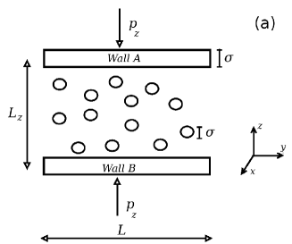
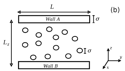
Figure 2: Schematic depiction of the simulation box with the fluid and walls. The walls are separated by a distance $L_{z}$, and have a size $\sigma$. The system with external pressure, $p_{z}$, and flexible walls is shown in (a) and the system with fixed walls in (b).

Here we study the structural and dynamic behavior of this fluid confined between two parallel plates. The simulation box is a parallelepiped with dimensions $L_{x}\times L_{y}\times L_{z}$. The model for the fluid-wall system is illustrated in Fig. 2. Two walls, A in the top and B in the bottom, are placed in the limits of the $z$-direction of the simulation box. These walls are treated as fixed in the Molecular Dynamics simulations performed at constant volume, and are allowed to move during the MD simulations realized with pressure control. The sizes $L_{x}$ and $L_{y}$ are fixed in all simulations, and defined as $L_{x}=L_{y}=L=20\sigma$. The values of $L_{z}$ were obtained first using $NpT$ simulations, where we have fixed the pressure $p_{z}$ in the $z$-direction using the Lupkowski and van Smol method of fluctuating confining walls LupSmol90 , as we show in Fig. 2(a). The $NVT$ ensemble simulations was performed with separations in the same range of the $<L_{z}>$ obtained in the $NpT$ simulations.

The walls are flat and purely repulsive. In order to represent the interaction between a fluid particle and these walls, we use the Weeks-Chandler-Andersen (WCA) potential.

$$U^{\rm{WCA}}(z_{ij})=\left\{\begin{array}[]{ll}U_{{\rm{LJ}}}(z_{ij})-U_{{\rm{LJ}}}(r_{c})\;,\qquad z_{ij}\leq r_{c}\;,\\ 0\;,\qquad\qquad\qquad\qquad\quad z_{ij}>r_{c}\;.\end{array}\right.$$ (2)

Here, $U_{{\rm{LJ}}}$ is the standard 12-6 LJ potential, included in the first term of Eq. (1), and $r_{c}=2^{1/6}\sigma$ is the usual cutoff for the WCA potential. Also, the term $z_{ij}$ measures the distance between the wall $j$ position and the $z$-coordinate of the fluid particle $i$.

II.2 The simulation details

The properties of the system were first evaluated with MD simulations at constant number of particles, pressure and temperature ($NpT$ ensemble). To fix the pressure in the $z$-direction, $p_{z}$, we have used the Lupkowski and van Smol method LupSmol90 . In this technique each wall has translational freedom in the confining direction and acts like a piston in the system, where a constant force controls the pressure in the $z$-direction.

The resulting force for a water like particles was then rewrite as

$$\vec{F}_{R}=-\vec{\nabla}U_{ij}+\vec{F}_{iwA}(\vec{r}_{iA})+\vec{F}_{iwB}(\vec{r}_{iB})\;,$$ (3)

where $\vec{F}_{iwj}$ indicates the interaction between the particle $i$ and the piston $j$.

Once the walls are allowed to move, we have to solve the equations of motion for the pistons $A$ and $B$,

$$m_{w}\vec{a}_{A}=p_{z}S_{w}\vec{n}_{A}-\sum_{i=1}^{N}\vec{F}_{iwA}(\vec{r}_{iA})$$ (4)

and

$$m_{w}\vec{a}_{B}=p_{z}S_{w}\vec{n}_{B}-\sum_{i=1}^{N}\vec{F}_{iwB}(\vec{r}_{iB})\;,$$ (5)

respectively, where $m_{w}$ is the piston mass, $p_{z}$ the desired pressure in the system, $S_{w}$ is the piston area and $\vec{n}_{A}$ is a unitary vector in positive $z$-direction, while $\vec{n}_{B}$ is a negative unitary vector. Both pistons ($A$ and $B$) have mass $m_{w}=m=1$, width $\sigma$ and area equal to $S_{w}=L^{2}$.

The system temperature was fixed using the Nose-Hoover heat-bath with a coupling parameter $Q=2$. Three values of temperature was chosen: one above the region in the phase diagram were the diffusion and the density of this fluid exhibit an anomalous behavior, $k_{B}T/\varepsilon=0.5$, a second and a third values inside of this anomalous region, $k_{B}T/\varepsilon=0.25$ and $k_{B}T/\varepsilon=0.15$ Oliveira06a . Standard periodic boundary conditions were applied in the $x$ and $y$ directions. The equations of motion for the particles of the fluid were integrated using the velocity Verlet algorithm, with a time step $\delta t=0.005$ in LJ time units.

The fluid-fluid interaction, Eq. (1), has a cutoff radius $r_{\rm cut}/\sigma=3.5$. The number of particles was fixed in $N=500$, and the pressure was varied from $p_{z}\sigma^{3}/\varepsilon=0.1$ to $p_{z}\sigma^{3}/\varepsilon=4.5$, with a $\delta p_{z}\sigma^{3}/\varepsilon=0.1$. For each pressure the systems equilibrate at different walls mean distance $<L_{z}>$. These displacement was used in the $NVT$ ensemble simulations. All the others parameters are equal to the used in the $NpT$ ensemble simulations.

Five independent runs were performed to evaluate the properties of the confined fluid. The initial system was generated placing the fluid particles randomly in the space between the walls. The initial displacement for the simulations with fluctuating wall was $L_{z0}=20\sigma$. We performed $5\times 10^{5}$ steps to equilibrate the system followed by $5\times 10^{6}$ steps for the results production stage. The equilibration time was taken in order to ensure that the pistons reached the equilibrium position for the fixed value of $p_{z}$. For the simulations with fixed walls the particles were placed randomly in the region between the walls, then equilibrated during $1\times 10^{6}$ steps followed by $2\times 10^{6}$ steps to obtain the physical quantities.

For calculating the lateral diffusion coefficient, $D_{||}$, we computed the mean square displacement (MSD) from Einstein relation

$$\langle[r_{||}(t)-r_{||}(t_{0})]^{2}\rangle=\langle\Delta r_{||}(t)^{2}\rangle=4Dt^{\alpha}\;,$$ (6)

where $r_{||}(t_{0})=(x(t_{0})^{2}+y(t_{0})^{2})^{1/2}$ and $r_{||}(t)=(x(t)^{2}+y(t)^{2})^{1/2}$ denote the parallel coordinate of the confined water-like molecule at a time $t_{0}$ and at a later time $t$, respectively. The diffusion coefficient $D_{||}$ is then obtained from

$$D_{||}=\lim_{t\to\infty}\frac{\langle\Delta r_{||}(t)^{2}\rangle}{4t^{\alpha}}\/.$$ (7)

Depending on the scaling law between $\Delta r_{||}^{2}$ and $t$ in the limit $t\rightarrow\infty$, different diffusion mechanisms can be identified: $\alpha=0.5$ identifies a single file regime Farimani11 , $\alpha=1.0$ stands for a Fickian diffusion whereas $\alpha=2.0$ refers to a ballistic diffusion Striolo06 ; Zheng12 .

III Results and Discussion

Case A: Fluctuating walls

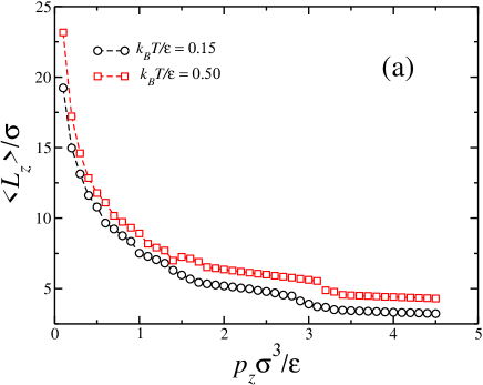
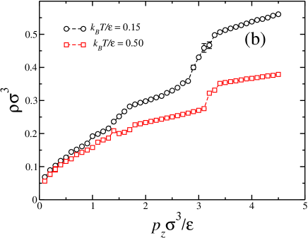
Figure 3: The distance $<L_{z}>$ between the walls in (a) and the density $\rho$ in (b) as function of the pressure applied by the walls in the $z$-direction for different values of temperature. Error bars are the deviation from the mean value. The results for $k_{B}T/\varepsilon=0.25$ are not shown here since they present the same behavior of $k_{B}T/\varepsilon=0.50$.

In a first moment we analyze the behavior of the water-like fluid when confined between two fluctuating walls. In the Fig. 3 we show how the separation $L_{z}$ between the walls in (a) and the fluid density $\rho$ in (b) vary with the applied pressure by the pistons. Since $\rho$ depends on $L_{z}$, both quantities exhibit the same behavior, with small jumps at certain values of $p_{z}$. The small error bars indicate that the walls perform short oscillations around the equilibrium position. In fact, for systems at $k_{B}T/\varepsilon=0.25$ and $0.50$ $,<L_{z}>$ do not exhibit any error bar larger than the data point, while for $k_{B}T/\varepsilon=0.15$ the density shows higher error bars in the region $p_{z}\sigma^{3}/\varepsilon\cong 3$. Also, the systems is more affected by the pressure for the smallest temperature. We can understand this as consequence of the competition between the external pressure pushing the walls and the opposite force generated by the fluid particles collisions with the wall at mean velocity $<v_{z}>=0.5k_{B}T$. To small values of temperature the pressure will act with a stronger intensity, while for higher values of $T$ the external force will be easily compensated by the particles collisions. Also, the jumps observed in the density behavior can be related to structural changes in the confined fluid. As we increase the pressure and decrease the space available for the fluid, their conformation and structure shift, leading to a abrupt change in the numbers of layers between the walls and to the observed jumps.

To illustrate the different layering observed, we show in Fig. 4(a) the density histogram in the confined direction for two values of wall displacement at temperature $k_{B}T/\varepsilon=0.15$. To obtain a better comparison the histograms were normalized, such that

$$\int\rho(z)\quad dz=1\;.$$ (8)

For large values of $<L_{z}>$, not shown here, the fluid structurates near the walls, as expected for hydrophobic surfaces, but in the center a liquid-like behavior is observed. When the system shows this structure, we assume that there is no layer formation. As we increase the pressure and decrease the separation between the walls we observe the formation of layers, as for $<L_{z}>/\sigma=5.4350$ and $<L_{z}>/\sigma=4.5502$, where the system exhibits 5 and 3 layers, respectively. The histogram for all the values of temperatures and walls displacement are not shown, but the behavior is similar. Since the temperature influences the layer formation, a distinct number of layers is observed for each value of $T$. The dependence of the number of layers with the distance between the walls for $k_{B}T/\varepsilon=0.15$ and $0.50$ is shown in Fig. 4(b). As expected, the fluid form layers at smaller values of $<L_{z}>$ for higher temperatures. The number of layers for $k_{B}T/\varepsilon=0.25$ is a intermediary case between the higher and lower temperature, and is not shown for simplicity.

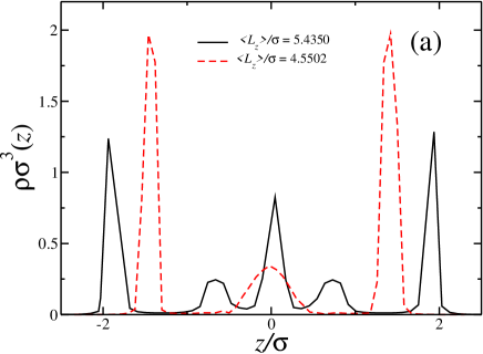
Figure 4: (a) Density histograms in the $z$-direction for some values of mean separation between the walls for systems at temperature $k_{B}T/\varepsilon=0.15$ and fluctuating walls. For simplicity, we do not show the histograms for the other temperatures. (b) Number of layers as function of $L_{z}/\sigma$ for different values of temperature. Zero layers indicates a fluid-like state.

The results obtained in our previous works for this water-like fluid confined between walls or inside nanotubes Krott13 ; Bordin12b ; Bordin13a show that, when the confining structure is rigid, the fluids assumes a structure where the mean distance between the layers in the confined direction is approximately 2. This is the characteristic distance of the second scale of the potential Eq. (1). However, in our simulations with fluctuating walls the distance between the layers can be 1, which is the characteristic distance of the first scale of the fluid-fluid interaction potential, or even smaller distances, as we can see in Fig. 4(a) for the cases with $<L_{z}>/\sigma=5.4350$ and $<L_{z}>/\sigma=4.5502$. This unusual behavior leads the system to present a non-monotonic behavior for the number of layers as function of $<L_{z}>$, Fig. 4(b), with an increase from 4 layers to 6 or 7 layers when $<L_{z}>/\sigma\cong 7.5$. To understand this effect we have to remember that the layer formation is resulted of the competition between the fluid-fluid interaction, Eq. (1), and the fluid-wall interaction, Eq. (2). As consequence, we can identify regimes where the system had a high organization, with the particles located at a distance equal to the second characteristic scale, and the enthalpic effects dominate over the entropic contribution for the free energy of the system. Also, the kinetic energy loss due the fluctuating walls favor the enthalpy, allowing the layers to accommodate at distances smaller than the second scale. As consequence, the system only exhibits a abrupt transitions from one number of layers to another, when the entropic contribution from the fluid-wall repulsion dominates. This lead to a smoother and continuous behavior of the self-diffusion coefficient as function of the plates separation, distinct to the one observed for this fluid when confined inside rigid nanotubes Bordin12b ; Bordin13a or inside fixed walls.

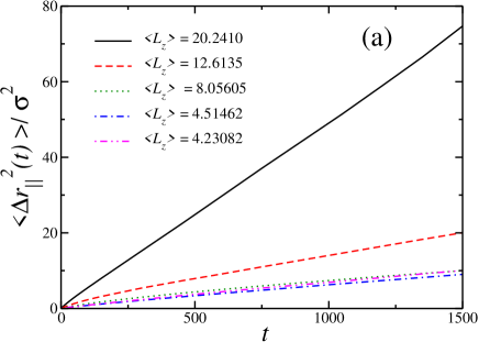
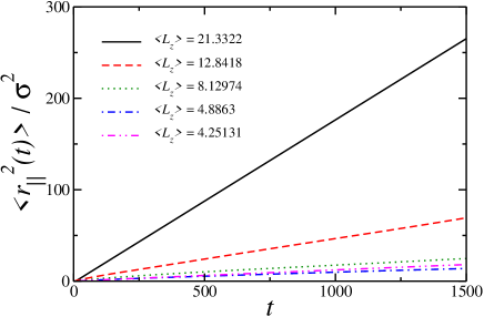
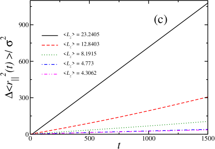
Figure 5: Parallel mean square displacement versus time for some values of wall displacement and for different values of temperature: (a) $k_{B}T/\varepsilon=0.15$, (b) $k_{B}T/\varepsilon=0.25$ and (c) $k_{B}T/\varepsilon=0.50$ and fluctuating walls. The errors bars not shown are smaller than the symbol size.

In order to understand the dynamical properties of this system we evaluate the MSD $\Delta r_{||}^{2}$ to check the diffusive regime of the fluid. In our model, we found $\alpha=1$, or a Fickian diffusion, for all plates displacement and for all temperatures, as shown in Fig. 5. The diffusion coefficient $D_{||}$ was then evaluated using the Eq. (7). We show the behavior of $D_{||}$ as function of the fluid density in Fig. 6. To maintain the graphics for different temperatures in the same scale we define $D_{0}$ as the value of the self diffusion coefficient at the smallest pressure for each isotherm. Our results indicates a rapid decrease in $D_{||}$ as we increase $\rho$ (or $p_{z}$), and then a saturation. The saturation occurs when the fluid assumes a layering structure and, after this, $D_{||}$ exhibits small fluctuations, that are related to changes in the number of layers of the confined fluid. This rapid saturation and the continuous and smooth shape of the curve for $D_{||}$ reinforce our assumption that the fluctuating walls favor the fluid to assume a structure that increases enthalpy and decreases the entropy, decreasing also the mobility. How the isotherms indicate, the temperature seems do not play a relevant role in this case, since the qualitative behavior is the same for all values of $k_{B}T/\epsilon$.

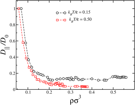
Figure 6: Dependence of the diffusion coefficient $D_{||}$ with the fluid density $\rho$ for systems with fluctuating walls. The system at $k_{B}T/\epsilon=0.25$ presented the same behavior of $k_{B}T/\epsilon=0.50$.

Is equally important to notice the absence of an anomalous behavior in the diffusion, characterized by a region where the diffusion coefficient increases as the density of the system increases. The diffusion anomaly was observed for all-atom models of water confined between hydrophobic fixed plates Zangi03b and inside nanotubes Farimani11 ; Zheng12 , and even for our water-like fluid model confined inside nanotubes Bordin12b . Our results indicates that allowing the walls to fluctuate, even when the fluctuation is small, lead to complete distinct results for the dynamical and structural behavior.

Case B: Fixed walls

Here we analyze systems confined between fixed walls, whose values of $L_{z}/\sigma$ were chosen in the same range of the mean values obtained for the fluctuating cases discussed in the last section.

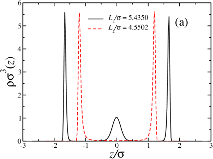
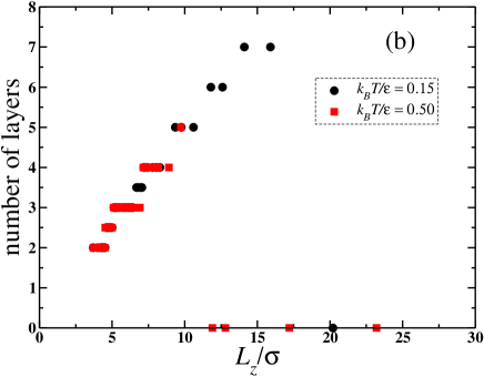
Figure 7: (a) Density histograms in the z-direction for some values of separation between the walls for systems at $k_{B}T/\varepsilon=0.15$ and fixed walls. (b) Number of layers as function of $L_{z}/\sigma$. Zero layers indicate a bulk-like behavior.

The formation of layers is shown in the Fig.7(a) through the density histograms for some values of $L_{z}/\sigma$, at $k_{B}T/\varepsilon=0.15$. Comparing these cases with those presented in the Fig.4(a), we verified that the structuration of the particles between the fixed walls are very different in relation to fluctuating cases at same mean values of $L_{z}/\sigma$. For $L_{z}/\sigma=5.4350$ and $4.5502$, the systems with fixed walls presented the formation of 3 and 2 layers, respectively, while for fluctuating cases, 5 and 3 layers were formed. The structuration of the fluid for both kinds of confinement is similar just for high distances between the walls.

The Fig.7(b) shows the number of layers formed for $k_{B}T/\varepsilon=0.15$ and $0.50$. The systems at $k_{B}T/\varepsilon=0.25$ are not shown for simplicity. Bulk-like systems occur for walls separated by high distances and they are indicated by zero layers. Broken numbers of layers, given by $2.5$ and $3.5$, indicate systems with formation of sublayers. A system with $2.5$ layers, for example, means the formation of two well defined contact layers and one middle layer with sublayers. When the systems change of a number of layers to another, presenting sublayers at intermediate cases, we called of layering transition. A two-to-three layers systems at $k_{B}T/\varepsilon=0.15$ are shown in the Fig.8. The same behavior is observed for $k_{B}T/\varepsilon=0.25$ and $0.50$. Since the walls are fixed, there is a limitation for the structuration of the particles between the walls. This favors the entropy and, as consequence, there will be the formation of sublayers. In counterpart, the fluctuation of the walls allows the accommodation of the particles in smaller distances, like the first scale of the fluid potential ($r/\sigma\sim 1$), as explained in last section. A transition between layers also was observed in systems like the SPC/E model confined between hydrophobic plates Giovambattista09 ; B805361H .

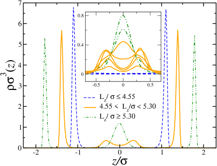
Figure 8: Density histograms showing the two-to-three layers transition at $k_{B}T/\varepsilon=0.15$ and fixed walls. The inset shows a zoom of the middle layer, where the formation of sublayers occurs.

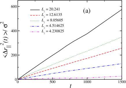
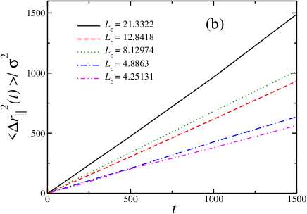
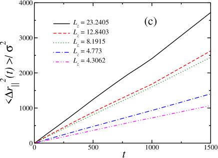
Figure 9: Mean square displacement for different separations between the plates at $k_{B}T/\varepsilon=0.15$ in (a), $k_{B}T/\varepsilon=0.25$ in (b) and $k_{B}T/\varepsilon=0.50$ in (c) in systems with fixed walls.

Besides the layering density, we also are interested to understand what happens with the dynamic of the systems when the walls are fixed. We show in Fig.9 the parallel mean square displacement ($\Delta r_{||}^{2}$) as function of time, for some values of $L_{z}/\sigma$ at $k_{B}T/\varepsilon=0.15$ in (a), $0.25$ in (b) and $0.50$ in (c). Like seen for fluctuating walls, the systems with fixed walls presented a Fickian diffusion regime, where $\alpha=1$. Considering that, the diffusion coefficient was calculated using the Eq. (7).

With the intuition to obtain a better understanding of the dynamical properties of the systems, we show in Fig.10(a) the diffusion coefficient normalized by $D_{0}$ as function of density. At low densities, ranged between $\rho\sigma^{3}\approx 0.100$ and $0.150$, an anomalous behavior in its diffusion is observed for the isotherms $k_{B}T/\varepsilon=0.15$ and $0.25$. At high temperatures, like $k_{B}T/\varepsilon=0.50$, this anomalous behavior almost disappears. The anomaly in the diffusion for this model already was observed in the bulk system Oliveira06a , in a previous work for confining rough fixed plates Krott13 and inside nanotubes Bordin12b . As we saw in the last section in Fig.6 (a) and (b), the anomalous behavior in the diffusion did not appear for fluctuating walls.

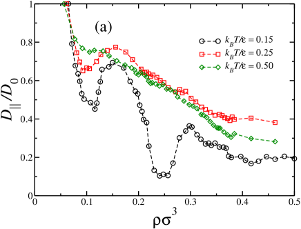
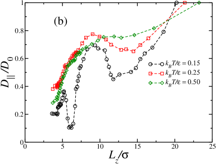
Figure 10: Dependence of the diffusion coefficient $D_{||}$ with fluid density $\rho$ in (a) and the distance $L_{z}/\sigma$ in (b) for systems with fixed walls.

Addictionally to the diffusion anomaly, we can observe an amorphous phase for some densities in the isotherm $k_{B}T/\varepsilon=0.15$. To clarify this behavior, we show in Fig.10(b) the diffusion coefficient as function of $L_{z}/\sigma$, and it is possible to see the values of $L_{z}/\sigma$ where the diffusion has a significant decrease, characterizing an amorphous behavior of the system. As example, we consider a system at $L_{z}/\sigma=5.200$, characterized by a liquid-like behavior, and other at $L_{z}/\sigma=6.435$, corresponding to an amorphous system. Both systems present the formation of three well defined layers, like we can see in the density histograms, in Fig.11(a). The structure of the system can be analyzed using the radial distribution function $g_{||}(r_{||})$ for each layer, defined as

$$g_{\parallel}(r_{\parallel})\equiv\frac{1}{\rho^{2}V}\sum_{i\neq j}\delta(r-r_{ij})\left[\theta\left(\left|z_{i}-z_{j}\right|\right)-\theta\left(\left|z_{i}-z_{j}\right|-\delta z\right)\right].$$ (9)

where the Heaviside function $\theta(x)$ restricts the sum of particle pair in a slab of thickness $\delta z=1.0$.

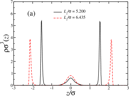
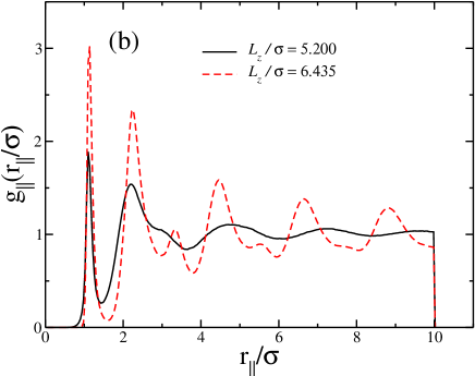
Figure 11: Case B: In (a), we show the density histograms for $L_{z}/\sigma=5.200$ and $6.435$ and in (b), we have the radial distribution function for the middle layer of $L_{z}/\sigma=5.200$ and $6.435$.

For systems with three well defined layers, we can calculate two $g_{||}(r_{||})$, one to each layer. The $g_{||}(r_{||})$ for the middle layer of the systems at $L_{z}/\sigma=5.200$ and $6.435$ is shown in Fig.11(b). The smooth behavior of the $g_{||}(r_{||})$ for $L_{z}/\sigma=5.200$ indicates a liquid-like structure, while the sharp peaks for $L_{z}/\sigma=6.435$ indicate a amorphous structure of the system. The $g_{||}(r_{||})$ for the contact layers are not shown because the conclusion about the structuration of the particles is the same. The systems at $L_{z}/\sigma=5.872$, $6.047$ and $6.197$ also presented amorphous behavior in their diffusion and structure. The solidification for some distances $L_{z}$ is supported by many works, using TIP5P Zangi03b ; Ku05b and SCP/E Giovambattista09 models.

IV Conclusion

We have studied the structural and dynamical behavior of a core-softened fluid confined between two walls. This fluid, in bulk, exhibits the thermodynamic, dynamic and structural anomalies observed in liquid water. We have consider two kinds of confinement. In the first, the walls are allowed to fluctuate, while in the second case the walls are fixed. In both systems the fluid-wall interaction is by excluded volume purely, and the wall is a simple planar plate. Our simulations shows that if we consider a system were the confining walls are free to move, fluctuating around the equilibrium position, the structure and the self diffusion of the fluid are different from the obtained for the case with fixed walls. The small fluctuations of the wall increase the entropic contribution to the free energy of the fluid, leading to structural conformations not observed when the confining media is fixed. Also, the diffusion coefficient diffusion shows a smooth dependence with the wall displacement, saturating when the system exhibits a layering. For fixed plates, besides the transition between layers and the diffusion anomaly, we observe a amorphous behavior for some values of $L_{z}$ at low temperature, $k_{B}T/\varepsilon=0.15$, what is not observed for the fluctuating cases. For small temperatures, the self-diffusion coefficient exhibits minimals, relates to this amorphous structure.

V Acknowledgments

This work was partially supported by the CNPq and CAPES.

References

- (1) M. Chaplin, Sixty-nine anomalies of water, http://www.lsbu.ac.uk/water/anmlies.html, 2013.
- (2) G. E. Karniadakis, A. Beskok, and N. R. Aluru, Microflows and Nanoflows - Fundamentals and Simulation, Springer Science+Business Media Inc, New York, 2005.
- (3) M. C. Bellissent-Funel and J. Teixeira, Structural an dynamic properties of bulk and confined water, L. Rey, New York, 2004.
- (4) J. K. Holt et al., Science 312, 1034 (2006).
- (5) J. SHen, J. Mater. Sci. 42, 6382 (2007).
- (6) Y. Zhang and H. Huang, Comput. Mater. Sci. 43, 664 (2008).
- (7) M. Elimelech and W. A. Philip, Science 333, 712 (2011).
- (8) T. A. Hilder, D. Gordon, and S. H. Chung, Nanomedicine 7, 702 (2011).
- (9) L. Liu, S. H. Chen, A. Faraone, C. W. Yen, and C. Y. Mou, Phys. Rev. Lett. 95, 117802 (2005).
- (10) F. Mallamace et al., J. Phys. Chem. B 114, 1870 (2010).
- (11) S. H. Chen et al., Proc. Ntl. Acad. Sci. U.S.A. 103, 12974 (2006).
- (12) T. G. Lombardo, N. Giovambattista, and P. G. Debenedetti, Faraday Discuss. 141, 359 (2008).
- (13) H. E. Stanley et al., J. Non. Crist. Solids 357, 629 (2011).
- (14) K. Koga, G. T. Gao, H. Tanaka, and X. C. Zeng, Nature 412, 802 (2001).
- (15) K. Koga, G. T. Gao, H. Tanaka, and X. C. Zeng, Physica A 314, 462 (2002).
- (16) M. Rovere and P. Gallo, The European Physical Journal E: Soft Matter and Biological Physics 12, 77 (2003).
- (17) I. Brovchenko, A. Geiger, A. Oleinikova, and D. Paschek, The European Physical Journal E: Soft Matter and Biological Physics 12, 69 (2003).
- (18) N. Giovambattista, P. J. Rossky, and P. G. Debenedetti, Phys. Rev. Lett. 102, 050603 (2009).
- (19) S. Han, M. Y. Choi, P. Kumar, and H. E. Stanley, Nature Phys. 6, 685 (2010).
- (20) P. Gallo, M. Rovere, and S.-H. Chen, Journal of Physics: Condensed Matter 24, 064109 (2012).
- (21) E. G. Strekalova, M. G. Mazza, H. E. Stanley, and G. Franzese, Journal of Physics: Condensed Matter 24, 064111 (2012).
- (22) A. Alexiadis and S. Kassinos, Chem. Eng. Sci. 63, 2093 (2008).
- (23) E. A. Jagla, Phys. Rev. E 58, 1478 (1998).
- (24) Z. Yan, S. V. Buldyrev, N. Giovambattista, and H. E. Stanley, Phys. Rev. Lett. 95, 130604 (2005).
- (25) L. Xu et al., Proc. Natl. Acad. Sci. U.S.A. 102, 16558 (2005).
- (26) A. B. de Oliveira, P. A. Netz, T. Colla, and M. C. Barbosa, J. Chem. Phys. 124, 084505 (2006).
- (27) A. B. de Oliveira, P. A. Netz, T. Colla, and M. C. Barbosa, J. Chem. Phys. 125, 124503 (2006).
- (28) N. M. B. Jr, E. Salcedo, and M. C. Barbosa, J. Chem. Phys. 131, 904509 (2009).
- (29) J. N. da Silva, E. Salcedo, A. B. de Oliveira, and M. C. Barbosa, J. Chem. Phys. 133, 244506 (2010).
- (30) P. H. Poole, F. Sciortino, U. Essmann, and H. E. Stanley, Nature (London) 360, 324 (1992).
- (31) L. Krott and M. C. Barbosa, J. Chem. Phys. 138, 084505 (2013).
- (32) J. R. Bordin, A. B. de Oliveira, A. Diehl, and M. C. Barbosa, J. Chem. Phys 137, 084504 (2012).
- (33) J. R. Bordin, A. Diehl, and M. C. Barbosa, J. Phys. Chem. B 117, 7047 (2013).
- (34) E. Strekalova et al., Journal of Biological Physics 38, 97 (2012).
- (35) Z. Mao and S. B. Sinnot, Phys. Rev. Lett. 89, 278301 (2002).
- (36) D. M. Ackerman, A. I. Skoulidas, D. S. Sholl, and J. K. Johnson, Mol. Simul. 29, 677 (2003).
- (37) X. Qin, Q. Yuan, Y. Zhao, S. Xie, and Z. Liu, Nanoletters 11, 2173 (2011).
- (38) M. Khademi and M. Sahimi, J. Chem. Phys 135, 204509 (2011).
- (39) K. P. Lee, H. Leese, and D. Mattia, Nanoscale 4, 2621 (2012).
- (40) R. Zangi and A. E. Mark, Phys. Rev. Lett. 91, 025502 (2003).
- (41) R. Zangi and A. E. Mark, J. Chem. Phys. 119, 1694 (2003).
- (42) P. Kumar, S. V. Buldyrev, F. W. Starr, N. Giovambattista, and H. E. Stanley, Phys. Rev. E 72, 051503 (2005).
- (43) S. Han, P. Kumar, and H. E. Stanley, Phys. Rev. E 77, 030201 (2009).
- (44) F. de los Santos and G. Franzese, The Journal of Physical Chemistry B 115, 14311 (2011).
- (45) F. de los Santos and G. Franzese, Phys. Rew. E 85, 010602 (2012).
- (46) E. de la Llave, V. Molinero, and D. A. Scherlis, J. of Phys. Chem. C 116, 1833 (2012).
- (47) H. B. Eral, D. van den Ende, F. Mugele, and M. H. G. Duits, Phys. Rev. E 80, 061403 (2009).
- (48) N. Choudhury, J. Chem. Phys. 132, 064505 (2010).
- (49) N. Giovambattista, P. J. Rossky, and P. G. Debenedetti, J. Phys. Chem. B 113, 13723 (2009).
- (50) P. Kumar, F. W. Starr, S. V. Buldyrev, and H. E. Stanley, Phys. Rev. E 72, 011202 (2007).
- (51) K. Koga, X. C. Zeng, and H. Tanaka, Phys. Rev. Lett. 72, 5262 (1997).
- (52) K. Koga, X. C. Zeng, and H. Tanaka, Che, Phys. Lett. 285, 278 (1998).
- (53) Q. Zhao, P. Majsztrik, and J. Benziger, J. Chem. Phys. B 115, 2717 (2011).
- (54) S. A. Eastman et al., Macromolecules 45, 7920 (2012).
- (55) B. G. Choi, J. Hong, W. H. Hong, P. T. Hammond, and H. Park, ACS Nano 5, 7205 (2011).
- (56) F. Salles et al., J. Phys. Chem. C 115, 10764 (2011).
- (57) H. Chen, J. K. Johnson, and D. S. Sholl, J. Phys. Chem. B Lett. 110, 1971 (2006).
- (58) S. Jakobtorweihen, M. G. Verbeek, C. P. Lowe, . F. J. Keil, and B. Smit, Phys. Rev. Lett. 95, 044501 (2005).
- (59) T. Mutat, J. Adler, and M. Sheintuch, J. Chem. Phys. 136, 234902 (2012).
- (60) M. Lupowski and F. van Smol, J. Chem. Phys. 93, 737 (1990).
- (61) P. Allen and D. J. Tildesley, Computer Simulation of Liquids, Oxford University Press, Oxford, 1987.
- (62) A. B. de Oliveira, E. Salcedo, C. Chakravarty, and M. C. Barbosa, J. Chem. Phys. 132, 234509 (2010).
- (63) G. S. Kell, J. Chem. Eng. Data 12, 66 (1967).
- (64) C. A. Angell, E. D. Finch, and P. Bach, J. Chem. Phys. 65, 3063 (1976).
- (65) A. B. Farimani and N. R. Aluru, J. Phys. Chem. B 115, 12145 (2011).
- (66) A. Striolo, Nanoletters 6, 633 (2006).
- (67) Y. Zheng, H. Ye, Z. Zhang, and H. Zhang, Phys. Chem. Chem. Phys. 14, 964 (2012).
- (68) T. G. Lombardo, N. Giovambattista, and P. G. Debenedetti, Faraday Discuss. 141, (2009).