Masses of the Bottom-Charm Hybrid $\bar{b}Gc$ States

Abstract

QCD sum rules are used to study the mass spectrum of bottom-charm hybrid $\bar{b}Gc$ systems. The correlation functions and the spectral densities are calculated up to dimension six condensates at leading order of $\alpha_{s}$ for several $J^{P}$ quantum numbers. After performing the QCD sum rule analysis, we predict the masses of the $J^{P}=0^{-},0^{+},1^{-},1^{+},2^{-},2^{+}$ bottom-charm hybrids. These mass predictions show a similar supermultiplet structure as the bottomonium and charmonium hybrids. Using the QCD sum-rule mass predictions we analyze the possible hadronic decay patterns of the $\bar{c}Gc$, $\bar{b}Gc$ and $\bar{b}Gb$ hybrids including the open-flavour and hidden-flavour mechanisms.

I Introduction

The existence of hybrid mesons was suggested by Jaffe and Johnson in 1976 Jaffe and Johnson (1976). Composed of a quark-antiquark pair and an excited gluonic field, hybrid mesons can carry exotic quantum numbers $J^{PC}=0^{--},0^{+-},1^{-+},2^{+-}$ etc. These exotic quantum numbers are not accessible for a quark-antiquark state, although hybrids can also have non-exotic quantum numbers and could in principle mix with quark-antiquark states. The observation of hybrids is one of the most important topics in hadronic physics, as evidenced by many experimental facilities such as PEPII, KEKB, BESIII, PANDA and LHCb that will search for hybrid mesons.

The spectrum of the light hybrid mesons was studied in several different approaches, such as the Bag model Barnes et al. (1983); Chanowitz and Sharpe (1983), the flux tube model Isgur et al. (1985); Close and Page (1995a); Barnes et al. (1995); Page et al. (1999); Close and Page (1995b), lattice QCD McNeile et al. (1999); Lacock and Schilling (1999); Bernard et al. (2003); Hedditch et al. (2005) and QCD sum rules Govaerts et al. (1983, 1984); Latorre et al. (1984, 1987); Balitsky et al. (1986); Jin et al. (2003); Chetyrkin and Narison (2000); Zhu (1999a). These approaches make very different mass predictions for the hybrids. To date, there has been some evidence of the exotic light hybrid with $J^{PC}=1^{-+}$ Thompson et al. (1997); Abele et al. (1998, 1999); Adams et al. (2007) (see Refs. Klempt and Zaitsev (2007); Ketzer (2012) for recent reviews). Some studies exist for heavy quarkonium hybrids in the constituent gluon model Horn and Mandula (1978), the flux tube model Barnes et al. (1995), QCD sum rules Govaerts et al. (1985a, b); Govaerts et al. (1987); Zhu (1999b); Qiao et al. (2012); Harnett et al. (2012); Berg et al. (2012), nonrelativistic QCD Chiladze et al. (2012) and lattice QCD Perantonis and Michael (1990); Juge et al. (1999); Liu and Luo (2006); Luo and Liu (2006); Liu et al. (2011, 2012). However, to our knowledge the bottom-charm hybrids have not been studied in any of these methods.

In a recent paper Chen et al. (2013), we have studied the charmonium and bottomonium hybrids $\bar{c}Gc$ and $\bar{b}Gb$ using the QCD sum rule method. We consider the following operators which couple to the hybrid states with definite $J^{P(C)}$ quantum numbers

$$J^{(1)}_{\mu} = g_{s}\bar{Q}_{1}\frac{\lambda^{a}}{2}\gamma^{\nu}G^{a}_{\mu\nu}Q_{2},~{}~{}~{}~{}~{}~{}~{}J^{PC}=1^{-(+)},0^{+(+)},$$

$$J^{(2)}_{\mu} = g_{s}\bar{Q}_{1}\frac{\lambda^{a}}{2}\gamma^{\nu}\gamma_{5}G^{a}_{\mu\nu}Q_{2},~{}~{}~{}~{}J^{PC}=1^{+(-)},0^{-(-)},$$ (1)

$$J^{(3)}_{\mu\nu} = g_{s}\bar{Q}_{1}\frac{\lambda^{a}}{2}\sigma_{\mu}^{\alpha}\gamma_{5}G^{a}_{\alpha\nu}Q_{2},~{}~{}~{}~{}J^{PC}=2^{-(+)},1^{+(+)},1^{-(+)},0^{-(+)}\,.$$

in which $Q_{1}$ and $Q_{2}$ are the heavy quark fields with masses $m_{1}$ and $m_{2}$, $g_{s}$ is the strong coupling constant, $\lambda^{a}$ are the Gell-Mann SU(3) matrices and $G^{a}_{\mu\nu}$ is the gluon field strength. It should be pointed out, however, the operators in Eq. (1) with $Q_{1}\neq Q_{2}$ carry no definite C-parities. The signs in the parentheses are the corresponding C-parities for the hidden flavour (equal mass) systems with $Q_{1}=Q_{2}$. By replacing $G^{a}_{\mu\nu}$ with $\tilde{G}^{a}_{\mu\nu}=\frac{1}{2}\epsilon_{\mu\nu\alpha\beta}G^{\alpha\beta,a}$, we can also obtain the corresponding operators $\tilde{J}^{(1)}_{\mu},\tilde{J}^{(2)}_{\mu},\tilde{J}^{(3)}_{\mu\nu}$ with opposite parities. These hybrid interpolating currents were originally studied to calculate the masses of the hidden flavour $\bar{c}Gc$ and $\bar{b}Gb$ hybrids for $Q_{1}=Q_{2}$ in Refs. Govaerts et al. (1985a); Govaerts et al. (1987) and the open flavour heavy-light $\bar{Q}Gq$ hybrids for $Q_{1}\neq Q_{2}$ in Ref. Govaerts et al. (1985b). However, only the perturbative and dimension four gluon condensate contributions were calculated for the correlation functions in these papers, which resulted in unstable hybrid sum rules and hence unreliable mass predictions for some channels. Recently, dimension-six condensates have been shown to stabilize the sum-rule mass predictions of the $J^{PC}=1^{--}$ Qiao et al. (2012), $1^{++}$ Harnett et al. (2012) and $0^{-+}$ Berg et al. (2012) channels. The dimension six contributions are thus very important because they stabilize the hybrid sum rules.

In Ref. Chen et al. (2013), we re-analyzed all the channels with $J^{PC}=0^{-+},0^{--},0^{++},0^{+-},1^{-+},1^{--},1^{+-},1^{++},2^{-+},2^{++}$ by including the tri-gluon condensate contributions and updated the mass spectrum of $\bar{c}Gc$ and $\bar{b}Gb$ hybrids, confirming the supermultiplet structures of the heavy quarkonium hybrid spectrum found in lattice QCD Liu et al. (2012) and the P-wave quasigluon approach Guo et al. (2008).

In this paper, we extend our investigation to $\bar{b}Gc$ ($\bar{c}Gb$) systems using the interpolating currents in Eq. (1) with $Q_{1}\neq Q_{2}$. In this situation, the $\bar{b}Gc$ type of currents in Eq. (1) couple to the charged hybrid states with no definite C-parities. This is very similar to the heavy-light hybrids studied in QCD sum rules Govaerts et al. (1985b) and lattice QCD Moir et al. (2013). With their special hadronic configuration, the mass prediction of the bottom-charm $\bar{b}Gc$ hybrids can provide important information for future experimental searches.

For the $\bar{b}Gc$ currents in Eq. (1), $J^{(1)}_{\mu}$ and $\tilde{J}^{(2)}_{\mu}$ both couple to the $J^{P}=1^{-},0^{+}$ states while $J^{(2)}_{\mu}$ and $\tilde{J}^{(1)}_{\mu}$ both couple to the $J^{P}=1^{+},0^{-}$ states. Although multiple operators exist for a given quantum number, they may have different couplings to the ground and excited states, so one should not necessarily expect the same mass predictions. Generally, the operator leading to the smallest mass prediction would provide the best determination of the ground state. For the spin-2 states, the tensor currents $J^{(3)}_{\mu\nu}$ and $\tilde{J}^{(3)}_{\mu\nu}$ couple to $J^{P}=2^{-}$ and $J^{P}=2^{+}$ channels respectively. We will calculate the correlation functions up to dimension six tri-gluon condensate contributions to perform the QCD sum rule analysis.

The paper is organized as follows. In Sec. ii@, we calculate the $\bar{b}Gc$ correlation functions and spectral densities using the hybrid interpolating currents with various quantum numbers in Eq. (1). In Sec. iii@, we perform the numerical analysis and extract masses of the $\bar{b}Gc$ hybrid states. We study the possible decay patterns of the $\bar{c}Gc$, $\bar{b}Gc$ and $\bar{b}Gb$ hybrids in Sec. iv@. The last section is a brief summary.

II QCD Sum Rule and Spectral Densities

In the past few decades, QCD sum rules have been widely used to study hadronic structures Shifman et al. (1979); Reinders et al. (1985); Colangelo (2000). We consider the two-point correlation function:

$$\Pi_{\mu\nu}(q)=i\int d^{4}xe^{iq\cdot x}\langle 0|T[J_{\mu}(x)J_{\nu}^{{\dagger}}(0)]|0\rangle,$$ (2)

where $J_{\mu}$ is the hybrid interpolating current in Eq. (1). Since these currents are not conserved, the two-point correlation functions have the following structures:

$$i\int d^{4}x\,e^{iq\cdot x}\,\langle 0|T[J_{\mu}(x)J_{\nu}^{\dagger}(0)]|0\rangle = \left[\frac{q_{\mu}q_{\nu}}{q^{2}}-g_{\mu\nu}\right]\Pi_{V}(q^{2})+\frac{q_{\mu}q_{\nu}}{q^{2}}\Pi_{S}(q^{2}),$$ (3)

$$i\int d^{4}x\,e^{iq\cdot x}\,\langle 0|T[J_{\mu\nu}(x)J_{\rho\sigma}^{{\dagger}}(0)]|0\rangle = \left[\eta_{\mu\rho}\eta_{\nu\sigma}+\eta_{\mu\sigma}\eta_{\nu\rho}-\frac{2}{3}\eta_{\mu\nu}\eta_{\rho\sigma}\right]\Pi_{T}(q^{2})+\ldots\,,$$ (4)

where $\eta_{\mu\nu}=q_{\mu}q_{\nu}/q^{2}-g_{\mu\nu}$. The imaginary parts of the invariant functions $\Pi_{V}(q^{2})$, $\Pi_{S}(q^{2})$ and $\Pi_{T}(q^{2})$ refer to pure spin-1, spin-0 and spin-2 intermediate states, respectively. In Eq. (4), the invariant structures for spin-0 and spin-1 are not written out explicitly because we will not consider contributions arising from these terms in this paper.

The correlation function can be described at both the hadron level and the quark-gluon level. To determine the correlation function at the hadron level, we use the dispersion relation

$$\Pi(q^{2})=\frac{(q^{2})^{N}}{\pi}\int_{(m_{1}+m_{2})^{2}}^{\infty}\frac{\mbox{Im}\Pi(s)}{s^{N}(s-q^{2}-i\epsilon)}ds+\sum_{n=0}^{N-1}b_{n}(q^{2})^{n},$$ (5)

where

$$\rho(s)\equiv\frac{1}{\pi}\mbox{Im}\Pi(s)=\sum_{n}\delta(s-m_{n}^{2})\langle 0|J_{\mu}|n\rangle\langle n|J_{\mu}^{\dagger}|0\rangle=f_{X}^{2}m_{X}^{8}\delta(s-m_{X}^{2})+\mbox{continuum},$$ (6)

in which we use a narrow resonance approximation and write the spectral function $\rho(s)$ (the imaginary part of $\Pi(s)$) as a sum over a series of zero-width $\delta$ functions. Finally, the pole plus continuum approximation is adopted to pick out the lowest lying resonance. The unknown subtraction constants $b_{n}$ in the right hand side of Eq. (5) can be removed by taking the Borel transform of $\Pi(q^{2})$. The intermediate states $|n\rangle$ must have the same quantum numbers as the interpolating currents $J_{\mu}$. In Eq. (6), $m_{X}$ denotes the mass of the lowest lying resonance, and the dimensionless quantity $f_{X}$ is the coupling of the resonance to the current

$$\langle 0|J_{\mu}|X\rangle = f_{X}m_{X}^{4}\epsilon_{\mu}\,,$$ (7)

$$\langle 0|J_{\mu\nu}|X\rangle = f_{X}m_{X}^{4}\epsilon_{\mu\nu}\,,$$ (8)

in which $\epsilon_{\mu}$ and $\epsilon_{\mu\nu}$ are the (spin-1) polarization vector and (spin-2) polarization tensor.

To evaluate the correlation function $\Pi(q^{2})$ at the quark-gluon level, we first need to determine the full quark propagator. For $\bar{b}Gc$ hybrid systems, the quark condensates and quark-gluon mixed condensates are expressed in terms of the gluon condensate and tri-gluon condensate via the heavy quark mass expansion and hence give no contributions to the correlation function. Taking into account only the gluon condensate and tri-gluon condensate contributions, we use the full quark propagator in momentum space Reinders et al. (1985)

$$iS_{ab}(p) = \frac{i\delta_{ab}}{\not{p}-m}+\frac{i}{4}g_{s}\frac{\lambda^{n}_{ab}}{2}G_{\mu\nu}^{n}\frac{\sigma^{\mu\nu}(\not{p}+m)+(\not{p}+m)\sigma^{\mu\nu}}{(p^{2}-m^{2})^{2}},$$ (9)

where $\sigma^{\mu\nu}=\frac{i}{2}\left[\gamma^{\mu}\,,\gamma^{\nu}\right]$, and $a\,,b$ are color indices. To calculate the Wilson coefficients at leading order in $\alpha_{s}$, the perturbative, gluon condensate $\langle\alpha_{s}GG\rangle$ and tri-gluon condensate $\langle g_{s}^{3}fGGG\rangle$ contributions are represented in Fig. II, Fig. II and Fig. II, respectively. In Fig. IIa, the condensate $\langle DDG\rangle$ can be expressed in terms of $\langle g_{s}^{3}fGGG\rangle$ and $\langle g_{s}^{4}jj\rangle$ by using the equation of motion, Bianchi identities and commutation relations. Within the vacuum factorization assumption, the contribution of $\langle g_{s}^{4}jj\rangle$ is proportional to the square of $g_{s}^{2}\langle\bar{q}q\rangle$ and thus will be neglected in this work since it is a small numerical effect compared to the gluonic condensates Chen et al. (2013).

Figure 1: Feynman diagram representing the perturbative contribution to the correlation functions. Solid and curly lines represent quark and gluon propagators respectively, while the dashed line represents the interpolating current.

Figure 2: Feynman diagram representing the $\langle\alpha_{s}GG\rangle$ contribution to the correlation functions.

(a)                                            (b)

Figure 3: Feynman diagrams representing the $\langle DDG\rangle$ (a) and $\langle g_{s}^{3}fGGG\rangle$ (b) contributions to the correlation functions.

Appendix A presents the results for the correlation functions and the spectral densities up to dimension six condensate contributions. From these expressions, we find that the perturbative contributions are invariant and the gluon condensate and tri-gluon condensate contributions change sign under the replacement $G^{a}_{\mu\nu}\to\tilde{G}^{a}_{\mu\nu}$ of the interpolating currents. For the same spin channels (spin-0 or spin-1), the specral densities from $J^{(1)}_{\mu}$ are identical to those from $J^{(2)}_{\mu}$ except for the additional minus signs for the odd power of the $m_{1}m_{2}$ proportional terms. For these formulae, it is straightforward to check that in the equal mass limit one recovers known results in Ref. Chen et al. (2013). Note the presence of $\delta(s-\tilde{m}^{2})$ and its derivatives in the tri-gluon condensate contributions (22) to compensate for the singular behavior of the spectral densities at threshold $s=(m_{1}+m_{2})^{2}$.

We can establish a sum rule for the hybrid mass by comparing the correlation function calculated at the quark-gluon level with those from the dispersion relation at the hadron level. The Borel transform is applied at both the quark-gluon and hadron levels to pick out the lowest lying resonance, eliminate the unknown subtraction constants in Eq. (5), and enhance the operator-product expansion (OPE) convergence. Using the spectral function in Eq. (6), we arrive at

$$f_{X}^{2}m_{X}^{8+2k}e^{-m_{X}^{2}/M_{B}^{2}}=\int_{(m_{1}+m_{2})^{2}}^{s_{0}}ds\,s^{k}\,\rho(s)\,e^{-s/M_{B}^{2}}=\mathcal{L}_{k}\left(s_{0},M_{B}^{2}\right)\,,$$ (10)

where $s_{0}$ is the continuum threshold parameter and $M_{B}$ is the Borel mass. Then we extract the hybrid mass via

$$m_{X}^{2}=\frac{\mathcal{L}_{1}\left(s_{0}\,,M_{B}^{2}\right)}{\mathcal{L}_{0}\left(s_{0}\,,M_{B}^{2}\right)}\,,$$ (11)

and the corresponding coupling constant via

$$f_{X}^{2}=\frac{\mathcal{L}_{0}\left(s_{0},M_{B}^{2}\right)}{m_{X}^{8}}e^{m_{X}^{2}/M_{B}^{2}},$$ (12)

in which $m_{X}$ denotes the $\bar{b}Gc$ hybrid mass as defined in Eq. (11).

III Numerical Analysis

We perform the QCD sum rule numerical analysis using the following values of the heavy quark masses and the condensates Chetyrkin et al. (2009); Narison (2012, 2010); Kuhn et al. (2007):

$$m_{c}(\mu=m_{c})=\overline{m}_{c}=(1.28\pm 0.02)~{}\mbox{GeV},$$

$$m_{b}(\mu=m_{b})=\overline{m}_{b}=(4.17\pm 0.02)~{}\mbox{GeV},$$

$$\langle\alpha_{s}GG\rangle=(7.5\pm 2.0)\times 10^{-2}~{}\mbox{GeV}^{4},$$

$$\langle g_{s}^{3}fGGG\rangle=-(8.2\pm 1.0)~{}\mbox{GeV}^{2}\langle\alpha_{s}GG\rangle,$$ (13)

in which the charm and bottom quark masses are the running masses in the $\overline{\rm MS}$ scheme. The definition of the coupling constant $g_{s}$ has a minus sign difference in this work. Furthermore, we take into account the scale dependence of these $\overline{\rm MS}$ masses in the leading order:

$$m_{c}(\mu)=\overline{m}_{c}\bigg{(}\frac{\alpha_{s}(\mu)}{\alpha_{s}(\overline{m}_{c})}\bigg{)}^{12/25},$$ (14)

$$m_{b}(\mu)=\overline{m}_{b}\bigg{(}\frac{\alpha_{s}(\mu)}{\alpha_{s}(\overline{m}_{b})}\bigg{)}^{12/23}\,,$$ (15)

where

$$\alpha_{s}(\mu) = \frac{\alpha_{s}(M_{\tau})}{1+\frac{25\alpha_{s}(M_{\tau})}{12\pi}\log(\frac{\mu^{2}}{M_{\tau}^{2}})},\quad\alpha_{s}(M_{\tau})=0.33,$$ (16)

is determined by evolution from the $\tau$ mass using Particle Data Group values Beringer et al. (2012). In the bottom-charm hybrid systems, there is a typical scale $\mu=\frac{\overline{m}_{c}+\overline{m}_{b}}{2}=2.73$ GeV which will be adopted in our sum rule analysis.

There are two very important parameters in the sum rules Eq. (10): the continuum threshold parameter $s_{0}$ and Borel mass $M_{B}$. To establish a reliable sum rule extracting the hybrid mass from Eq. (11), one should obtain suitable working regions of these two parameters. In our analysis, we choose the value of $s_{0}$ around which the variation of the hybrid mass $m_{X}$ with $M_{B}^{2}$ is minimum. The Borel window is determined by the convergence of the OPE series and the pole contribution. The lower bound on $M_{B}^{2}$ is determined by imposing that the gluon condensate contribution is less than one fourth of the perturbative contribution while the tri-gluon condensate contribution is less than one fourth of the gluon condensate contribution. Requiring the pole contribution to be larger than $50\%$, we obtain the upper bound on $M_{B}^{2}$.

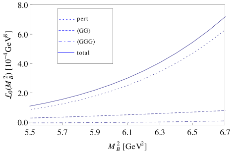
Figure 4: The contributions of each term in OPE series, including the perturbative term, gluon condensate $\langle\alpha_{s}GG\rangle$ and tri-gluon condensate $\langle g_{s}^{3}fGGG\rangle$ for the $\bar{b}Gc$ hybrid with $J^{P}=1^{-}$ by using $\tilde{J}^{(2)}_{\mu}$.

The definition of the pole contribution (PC) is

$$\mbox{PC}(s_{0},M_{B}^{2})=\frac{\mathcal{L}_{0}\left(s_{0}\,,M_{B}^{2}\right)}{\mathcal{L}_{0}\left(\infty\,,M_{B}^{2}\right)}.$$ (17)

We first study the $J^{P}=1^{-}$ $\bar{b}Gc$ hybrid by using the interpolating current $\tilde{J}^{(2)}_{\mu}$. The dominant non-perturbative contribution is the gluon condensate. After studying the OPE series, we show the OPE convergence for this channel in Fig. III, from which we determine the lower bound on the Borel mass as $M^{2}_{\mbox{min}}=5.9$ GeV². In Fig. III, we show the variations of the hybrid mass $m_{X}$ with the threshold parameter $s_{0}$ and the Borel mass $M_{B}^{2}$ for this channel. From the left plot, we choose the threshold parameter $s_{0}=52$ GeV² around which the variation of $m_{X}$ with $M_{B}^{2}$ is very weak, as shown in the right plot of Fig. III. Considering the constraint of the pole contribution, we obtain the upper bound of the Borel mass $M^{2}_{\mbox{max}}=6.5$ GeV². In this Borel window, we extract the mass for the $J^{P}=1^{-}$ $\bar{b}Gc$ hybrid

$$m_{X}=6.83\pm 0.08\pm 0.01\pm 0.07~{}\text{GeV},$$ (18)

in which the errors come respectively from the continuum threshold $s_{0}$, the heavy quark masses $m_{c},m_{b}$ and the gluon condensates $\langle\alpha_{s}GG\rangle,\langle g_{s}^{3}fGGG\rangle$. The error from the Borel mass $M_{B}$ is negligible since the mass sum rules is very stable in the Borel window (See Fig. III and Fig. III).

We can also explore the $1^{-}$ $\bar{b}Gc$ hybrid using the interpolating current $J^{(1)}_{\mu}$ in Eq. (1). To obtain a significant Borel window for this channel, we relax the constraint by requiring the pole contribution be larger than $20\%$. This requirement of the pole contribution also occurs in two $0^{-}$ channels, $2^{-}$ and $2^{+}$ channels, $0^{+}$ channel for the current $\tilde{J}^{(2)}_{\mu}$. Performing the same analysis as done above, we obtain the Borel window $9.00\,{\rm GeV^{2}}\leq M_{B}^{2}\leq 10.7$ GeV² while $s_{0}=62$ GeV² for $J^{(1)}_{\mu}$ with $J^{P}=1^{-}$. In contrast, we extract the hybrid mass $m_{X}=6.95\pm 0.13\pm 0.01\pm 0.08$ GeV, which is $0.12$ GeV lower than the $1^{-}$ hybrid mass extracted from $\tilde{J}^{(2)}_{\mu}$. The Borel curves are shown in Fig. III and the numerical results in Table III.

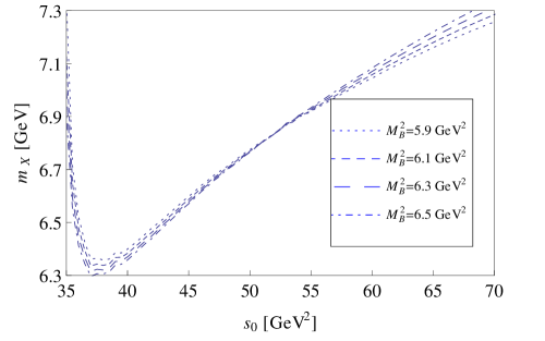
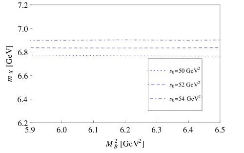
Figure 5: The variations of the hybrid mass $m_{X}$ with $s_{0}$ and $M_{B}^{2}$ for the $J^{P}=1^{-}$ channel by using $\tilde{J}^{(2)}_{\mu}$.

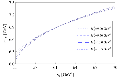
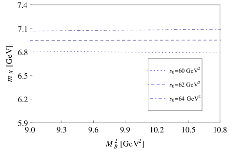
Figure 6: The variations of the hybrid mass $m_{X}$ with $s_{0}$ and $M_{B}^{2}$ for the $J^{P}=1^{-}$ channel by using $J^{(1)}_{\mu}$.

Using the spectral densities listed in Appendix A, we perform the sum rule analyses for the other $\bar{b}Gc$ hybrids with $J^{P}=0^{-},0^{+},1^{+},2^{-},2^{+}$. All these channels are stable enough to choose the suitable Borel windows among which one can establish reliable sum rules to extract the hybrid masses. We collect the numerical results including the hybrid masses, the threshold values, the Borel windows and the pole contributions in Table III. In cases where there exist multiple currents for the same quantum numbers, differences in the mass predictions imply that the currents differ in their relative couplings to the ground and excited state. The lowest mass prediction should be interpreted as the best determination of the ground state. As mentioned above, the errors of mass predictions come from the uncertainties in $s_{0}$, $m_{c}$ and $m_{b}$, $\langle\alpha_{s}GG\rangle$ and $\langle g_{s}^{3}fGGG\rangle$ respectively. One notes that both the errors from $s_{0}$ and the condensates $\langle\alpha_{s}GG\rangle,\langle g_{s}^{3}fGGG\rangle$ are important for mass predictions of two $1^{-}$ channels, lower $0^{-}$ and $0^{+}$ channels and $2^{-}$ channel. For the other channels, however, the main errors are from the uncertanties of QCD condensates. The errors from the heavy quark masses are very small for all channels.

	Operator	$J^{P}$	$s_{0}(\mbox{GeV}^{2})$	$[M^{2}_{\mbox{min}}$,$M^{2}_{\mbox{max}}](\mbox{GeV}^{2})$	$m_{X}$(GeV)	PC(%)	$f_{X}^{2}(10^{-7})$
	$\tilde{J}^{(2)}_{\mu}$	$1^{-}$	52	$5.90\sim 6.50$	$6.83\pm 0.08\pm 0.01\pm 0.07$	55.9	$0.77\pm 0.08\pm 0.05\pm 0.17$
	$\tilde{J}^{(1)}_{\mu}$	$0^{-}$	61	$10.4\sim 11.5$	$6.90\pm 0.12\pm 0.01\pm 0.09$	23.4	$2.21\pm 0.42\pm 0.16\pm 0.22$
	$J^{(1)}_{\mu}$	$1^{-}$	62	$9.00\sim 10.7$	$6.95\pm 0.13\pm 0.01\pm 0.08$	26.1	$1.74\pm 0.37\pm 0.14\pm 0.49$
	$J^{(3)}_{\mu\nu}$	$2^{-}$	59	$8.00\sim 10.5$	$7.15\pm 0.08\pm 0.05\pm 0.09$	29.4	$0.43\pm 0.07\pm 0.01\pm 0.10$
	$\tilde{J}^{(2)}_{\mu}$	$0^{+}$	69	$10.9\sim 12.0$	$7.37\pm 0.12\pm 0.07\pm 0.12$	22.8	$0.87\pm 0.17\pm 0.01\pm 0.23$
	$\tilde{J}^{(3)}_{\mu\nu}$	$2^{+}$	66	$8.00\sim 11.2$	$7.67\pm 0.07\pm 0.02\pm 0.09$	39.8	$0.51\pm 0.10\pm 0.04\pm 0.04$
	$J^{(2)}_{\mu}$	$1^{+}$	71	$5.90\sim 8.00$	$7.77\pm 0.06\pm 0.05\pm 0.13$	59.4	$2.19\pm 0.34\pm 0.02\pm 0.57$
	$\tilde{J}^{(1)}_{\mu}$	$1^{+}$	77	$9.00\sim 10.0$	$8.28\pm 0.05\pm 0.02\pm 0.31$	54.3	$4.99\pm 0.52\pm 0.03\pm 0.88$
	$J^{(1)}_{\mu}$	$0^{+}$	84	$10.4\sim 12.2$	$8.55\pm 0.05\pm 0.02\pm 0.37$	55.7	$7.14\pm 0.62\pm 0.02\pm 0.86$
	$J^{(2)}_{\mu}$	$0^{-}$	76	$10.9\sim 14.2$	$8.48\pm 0.04\pm 0.04\pm 0.59$	24.4	$1.29\pm 0.16\pm 0.02\pm 0.34$

Table 1: Masses of the $\bar{b}Gc$ hybrid states and the corresponding $s_{0}$, Borel windows, pole contributions and operator-state overlap.

To study the sensitivity of the hybrid sum rules to the values of gluon and tri-gluon condensates, we reanalyze the $\tilde{J}^{(2)}_{\mu}$ channel with $J^{P}=1^{-}$ by adopting another set of condensate values from Ioffe’s recent review Ioffe (2006): $\langle\alpha_{s}GG\rangle=(0.016\pm 0.013)$ GeV⁴, $\langle g_{s}^{3}fGGG\rangle=-4.69\langle\alpha_{s}GG\rangle$ GeV²=$-(0.075\pm 0.061)$ GeV⁶. For the current $\tilde{J}^{(2)}_{\mu}$ with $J^{P}=1^{-}$, the working regions of the hybrid sum rule with the above condensate values are $s_{0}=51$ GeV² and $4.1$ GeV² $\leq M_{B}^{2}\leq 4.7$ GeV². This Borel window is quite different with that obtained in Table III while the continuum threshold $s_{0}$ is very similar. We show the variations of the hybrid mass with $s_{0}$ and $M_{B}^{2}$ for $\tilde{J}^{(2)}_{\mu}$ channel with $J^{P}=1^{-}$ in Fig. III. The hybrid mass is extracted as $m_{X}=6.69$ GeV, which is slightly lower than that obtained in Table III using Narison’s condensate values Narison (2012, 2010).

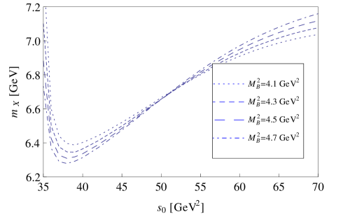
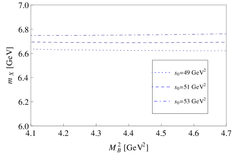
Figure 7: The variations of the hybrid mass $m_{X}$ with $s_{0}$ and $M_{B}^{2}$ for $\tilde{J}^{(2)}_{\mu}$ channel with $J^{P}=1^{-}$ adopting Ioffe’s condensate values Ioffe (2006).

In the MIT bag model Barnes et al. (1983); Chanowitz and Sharpe (1983), the hybrids with $J^{PC}=(0,1,2)^{-+},1^{--}$ were predicted to form the lightest hybrid supermultiplet consisting of a S-wave quark-antiquark pair coupled to an excited gluonic field with $J_{g}^{P_{g}C_{g}}=1^{+-}$. A higher hybrid supermultiplet composed of a P-wave $q\bar{q}$ pair and the same gluonic excitation would contain states with $J^{PC}=0^{+-},(1^{+-})^{3},(2^{+-})^{2},3^{+-},(0,1,2)^{++}$, where the superscript denotes the number of such states Liu et al. (2012); Dudek (2011). These hybrid supermultiplet structures were confirmed for the heavy quark sector in lattice QCD Liu et al. (2012), the P-wave quasigluon approach Guo et al. (2008) and QCD sum-rules Chen et al. (2013) with charmonium and bottomonium interpolating currents in Eq. (1). In Ref. Chen et al. (2013) the mass of the hybrid with $J^{PC}=0^{--}$ is very high, which may imply a different type of gluonic excitation.

These supermultiplet structures still exist in the $\bar{b}Gc$ hybrid systems. In Table III, the hybrid states with $J^{P}=(0,1,2)^{-},1^{-}$ form the lightest supermultiplet while the states with $J^{P}=(0^{+})^{2},(1^{+})^{2},2^{+}$ form a heavier supermultiplet. The heaviest state is a hybrid with $J^{P}=0^{-}$. The two $1^{-}$ hybrids lie very close since both of them belong to the lightest hybrid supermultiplet. In the heavier supermultiplet, there are two $1^{+}$ hybrids and two $0^{+}$ hybrids. The mass differences are $0.53$ GeV and $1.18$ GeV for $1^{+}$ and $0^{+}$, respectively. The mass difference of about $1.58$ GeV between the two $J^{P}=0^{-}$ hybrids is very large, suggesting that the operators are separately probing a ground and excited state. Our interpretation is that these two hybrids have very different gluonic excitations. However, further investigations in other methods are needed to understand the physics of $\bar{b}Gc$ hybrids.

The bottom-charm hybrids are not eigenstates of C-parity and G-parity, so the flavourless hybrids with $J^{PC}=J^{\pm\pm}$ and $J^{\pm\mp}$ have the same quantum numbers in the bottom-charm sector and thus can mix. For example, the interpolating currents $J^{(1)}_{\mu}$ and $\tilde{J}^{(2)}_{\mu}$ for the charmonium $\bar{c}Gc$ systems can couple to $1^{-+}$ and $1^{--}$ channels respectively and represent totally different channels with opposite C-parity and G-parity. In the MIT bag model Barnes et al. (1983); Chanowitz and Sharpe (1983), these two states have different spin configurations of the $\bar{q}q$ basis. The $1^{--}$ channel has a spin-singlet $S=0$ $\bar{q}q$ pair while $1^{-+}$ channel contains a spin-triplet $S=1$ $\bar{q}q$ pair. For the $\bar{b}Gc$ systems, however, they couple to the same $1^{-}$ bottom-charm channel, so it is not surprising that we obtain two $1^{-}$ states in Table III.

We can also perform a similar sum rule analysis for the coupling constant $f_{X}$ using Eq. (12), in which the hybrid mass $m_{X}$ can be expressed as in Eq. (11). In the coupling sum rules, we use the same criteria as those in the mass sum rules to obtain the working regions of $s_{0}$ and $M_{B}^{2}$. The lower bound on $M_{B}^{2}$ determined from the OPE convergence is unchanged. Now we perform an analysis of the coupling constant $f_{X}^{2}$ as a function of $s_{0}$. In the left portion of Fig. III, we show the variation of $f^{2}_{X}$ with $s_{0}$ for the $\tilde{J}^{(2)}_{\mu}$ channel with $J^{P}=1^{-}$. In this figure, the optimized choice of the continuum threshold is $s_{0}=49$ GeV², around which the variation of $f^{2}_{X}$ with the Borel mass $M_{B}$ is minimum. This value is very close to that obtained in the mass sum rules for the same channel. Since the upper bound on $M_{B}^{2}$ is only determined by the value of $s_{0}$, the Borel window in the coupling sum rules is almost the same as that obtained in the mass sum rules. After performing the numerical analysis, we find that this situation occurs in all channels. We show the variation of $f^{2}_{X}$ with $M_{B}^{2}$ for $\tilde{J}^{(2)}_{\mu}$ channel with $J^{P}=1^{-}$ in the right portion of Fig. III, which demonstrates that the Borel curve is very stable in the working region of Borel mass. For convenience but no loss of generality, we can use the same working regions of $s_{0}$ and $M_{B}^{2}$ as those utilized in the mass sum rules to predict the coupling constant $f_{X}$. The coupling constants for all channels are then calculated and collected in Table III. The error sources are the same as those in the mass predictions.

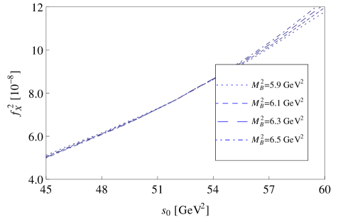
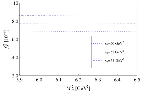
Figure 8: The variations of $f^{2}_{X}$ with $s_{0}$ and $M_{B}^{2}$ for $\tilde{J}^{(2)}_{\mu}$ channel with $J^{P}=1^{-}$.

IV Decay Patterns of the $\bar{c}Gc$, $\bar{b}Gc$ and $\bar{b}Gb$ Hybrids

In this section, we study the decay patterns of the possible $\bar{b}Gc$, $\bar{b}Gb$, and $\bar{c}Gc$ hybrid states using the mass predictions obtained in Table III and Ref. Chen et al. (2013). We just consider the two-body hadronic decays. Both the open flavour and hidden flavour deacy modes are taken into account.

According to some model-dependent analyses in Refs. Isgur and Paton (1985); Isgur et al. (1985); Close and Page (1995b); Kou and Pene (2005); Zhu (1999c); Close and Page (2005), hybrid mesons prefer to decay into $S+P$-wave final states. For example, the decay modes to pairs of identical $S$-wave mesons might be suppressed as shown in Refs. Kou and Pene (2005); Zhu (1999c); Close and Page (2005). For the charmonium hybrids, this implies that the $D\bar{D},D^{*}\bar{D}^{*}$ and $D_{s}\bar{D}_{s},D^{*}_{s}\bar{D}^{*}_{s}$ decay modes are suppressed while $D^{*}\bar{D}$ and $D^{*}_{s}\bar{D}_{s}$ are very small. The $D^{(*)}\bar{D}^{*}_{0}$ and $D^{(*)}\bar{D}_{1}$ channels would be the dominant decay modes if the hybrids are above their thresholds. In the MIT bag model Barnes et al. (1983); Chanowitz and Sharpe (1983), the $q\bar{q}$ pairs in hybrid mesons with $J^{PC}=1^{--},0^{++},1^{++},2^{++}$ are in a net spin singlet configuration. These hybrid mesons are forbidden to decay into final states consisting only of spin singlet mesons due to the spin selection rule Page et al. (1999).

Using the masses predicted in Ref. Chen et al. (2013), we collect the possible $S$-wave and $P$-wave decay modes of the charmonium hybrids in Table IV by taking account into the conservation of quantum numbers and the selection rules mentioned above. All the open charm decay modes should be understood as containing the charge conjugation parts. We have not listed the $D^{(*)}_{s}\bar{D}^{(*)}_{s}$ decay modes in Table IV because they are similar to the $D^{(*)}\bar{D}^{(*)}$ channels. One notes that the charmonium hybrids with $J^{PC}=1^{--},0^{-+},1^{-+}$, which belong to the lightest supermultiplet, lie below the open charm $D^{(*)}\bar{D}^{(*)}$ thresholds. They just decay via the hidden charm mechanism. The positive-parity states with $J^{PC}=1^{+-},(0,1,2)^{++}$ belong to the heavier hybrid supermultiplet. They lie above the open charm thresholds. According to the $S+P$-wave selection rule, they prefer the $D^{(*)}\bar{D}^{*}_{0}$ and $D^{(*)}\bar{D}_{1}$ decays. In Table IV, these decay modes are the $P$-wave coupling channels. These features are very different from the conventional $c\bar{c}$ mesons and the other exotic configurations such as the tetraquarks $cq\bar{c}\bar{q}$ and molecules $c\bar{q}\bar{c}q$, for which the $S$-wave $D\bar{D},D^{*}\bar{D}^{*},D\bar{D}^{*}$ channels are favoured. If the charmonium hybrids $\bar{c}Gc$ are predicted above the $D^{(*)}\bar{D}^{*}_{0}$ and $D^{(*)}\bar{D}_{1}$ thresholds, the observation of the anomalous branching ratios in these different channels could be understood as a strong hybrid signature Close and Page (1995b); Barnes et al. (1995); Close and Page (2005).

$I^{G}J^{PC}$	$S$-wave	$P$-wave
$0^{-}1^{--}$	$-$	$-$
$0^{+}0^{-+}$	$\eta_{c}(1S)f_{0}(600)$	$-$
$0^{+}1^{-+}$	$-$	$\eta_{c}(1S)\eta,J/\psi\omega(782)$
$0^{+}2^{-+}$	$-$	$D\bar{D}^{*},J/\psi\omega(782)$
$0^{-}0^{+-}$	$-$	$J/\psi f_{0}(600)$
$0^{+}2^{++}$	$J/\psi\omega(782),J/\psi\phi(1020),$	$D\bar{D}_{1},D\bar{D}_{2}^{*},D^{*}\bar{D}_{0}^{*},D^{*}\bar{D}_{1},D^{*}\bar{D}_{0}^{*},$
	$\chi_{c2}(1P)f_{0}(600)$	$J/\psi h_{1}(1170),\eta_{c}(1S)f_{1}(1285),\eta_{c}(1S)f_{2}(1270),$
		$\chi_{c1}(1P)\eta,\chi_{c2}(1P)\eta$
$0^{-}1^{+-}$	$D\bar{D}^{*},J/\psi\eta,\psi(2S)\eta,\chi_{c0}(1P)h_{1}(1170)$	$D\bar{D}_{0}^{*},D\bar{D}_{1},D\bar{D}_{2}^{*},D^{*}\bar{D}_{0}^{*},D^{*}\bar{D}_{2}^{*},D^{*}\bar{D}_{1},$
		$\eta_{c}(1S)h_{1}(1170),\eta_{c}(2S)h_{1}(1170)$
$0^{+}1^{++}$	$D\bar{D}^{*},D^{*}_{0}\bar{D}_{1},D_{1}\bar{D}_{2}^{*},J/\psi\omega(782),$	$D\bar{D}_{0}^{*},D\bar{D}_{1},D\bar{D}_{2}^{*},D^{*}\bar{D}_{0}^{*},D^{*}\bar{D}_{2}^{*},D^{*}\bar{D}_{1},$
	$J/\psi\phi(1020),\chi_{c0}(1P)f_{1}(1285),$	$\eta_{c}(1S)f_{0}(600),\eta_{c}(1S)f_{0}(980),\eta_{c}(2S)f_{0}(600),$
	$\chi_{c1}(1P)f_{0}(600),\chi_{c2}(1P)f_{1}(1285)$	$\eta_{c}(2S)f_{0}(980),\eta_{c}(1S)f_{1}(1285),\eta_{c}(1S)f_{2}(1270),$
		$J/\psi h_{1}(1170),\chi_{c(0,1,2)}(1P)\eta$
$0^{+}0^{++}$	$J/\psi\omega(782),J/\psi\phi(1020),\eta_{c}(1S)\eta,\eta_{c}(2S)\eta,$	$D\bar{D}_{1},D^{*}\bar{D}_{0}^{*},D^{*}\bar{D}_{1},D^{*}\bar{D}_{2}^{*},$
	$\chi_{c0}(1P)f_{0}(600),\chi_{c0}(1P)f_{0}(980),$	$\eta_{c}(1S)f_{1}(1285),\eta_{c}(2S)f_{1}(1285),J/\psi h_{1}(1170),$
	$\chi_{c1}(1P)f_{1}(1285),\chi_{c2}(1P)f_{2}(1270)$	$\psi(2S)h_{1}(1170),\chi_{c1}(1P)\eta$
$0^{-}0^{--}$	$D\bar{D}_{0}^{*},D^{*}\bar{D}_{1},J/\psi f_{1}(1285),$	$D\bar{D}^{*},D_{0}^{*}\bar{D}_{1},D_{1}\bar{D}_{2}^{*},J/\psi\eta,\psi(2S)\eta,$
	$\psi(2S)f_{1}(1285),\chi_{c1}(1P)\omega(782)$	$\eta_{c}(1S)\omega(782),\eta_{c}(2S)\omega(782),\chi_{c(0,1,2)}(1P)h_{1}(1170)$

Table 2: The possible decay modes of the charmonium hybrids with various quantum numbers.

Replacing the D and charmonium mesons by the B and bottomonium mesons respectively, we obtain the decay patterns of the bottomonium hybrids in Table IV so long as the kinematics allows. We note that the masses of the bottomonium hybrids with $J^{PC}=1^{--},0^{-+},1^{-+},2^{-+}$ in the lightest supermultiplet are lower than the open bottom $B^{(*)}\bar{B}^{(*)}$, $B_{s}{(*)}\bar{B}_{s}^{(*)}$ thresholds and one bottomonium meson plus one light meson thresholds. They cannot decay into the two-body final states through neither open bottom nor hidden bottom mechanisms. Once produced, they only decay via the electromagnetic and weak interactions.

The decay mechanism of the $\bar{b}Gc$ hybrids will be different from the $\bar{c}Gc$ and $\bar{b}Gb$ states. The selection rule forbidding $S+S$-wave final states no longer works in this situation because the internal structures and sizes of the $D$ and $B$ mesons differ Close and Page (1995b, a); Swanson and Szczepaniak (1997). The $B^{(*)}D^{(*)}$ and $B_{s}^{(*)}D_{s}^{(*)}$ open flavour decay modes are prefered for the $\bar{b}Gc$ hybrids above these thresholds. Besides, there will be no constraints of the C-parity and G-parity as for the $\bar{c}Gc$ and $\bar{b}Gb$ hybrids since the $\bar{b}Gc$ hybrids are not enginstates of C-parity and G-parity. We collect the possible decay patterns of the $\bar{b}Gc$ hybrids in Table IV. The PDG mass of the pesudoscalar $B_{c}$ meson is $m_{B_{c}}=6.277\pm 0.006$ GeV Beringer et al. (2012). To date, the other bottom-charm $B_{c}$ mesons have not been observed. To predict the hidden flavour decays of the $\bar{b}Gc$ hybrids, we use the masses of the vector ($B_{c}^{*}$), scalar ($B_{c0}$), axialvector ($B_{c1}$) and tensor ($B_{c2}$) bottom-charm mesons predicted in lattice QCD Davies et al. (1996): $m_{B_{c}^{*}}=6.321$ GeV, $m_{B_{c0}}=6.727$ GeV, $m_{B_{c1}}=6.743$ GeV and $m_{B_{c2}}=6.783$ GeV. In contrast to the $\bar{c}Gc$ and $\bar{b}Gb$ hybrids, more decay modes are alowed and the $S+S$-wave pair decays are dominant.

$I^{G}J^{PC}$	$S$-wave	$P$-wave
$0^{-}1^{--}$	$-$	$-$
$0^{+}0^{-+}$	$-$	$-$
$0^{+}1^{-+}$	$-$	$-$
$0^{+}2^{-+}$	$-$	$-$
$0^{-}0^{+-}$	$-$	$\Upsilon(1S)f_{0}(600)$
$0^{+}2^{++}$	$\Upsilon(1S)\omega(782),\Upsilon(1S)\phi(1020),\chi_{b2}(1P)f_{0}(600)$	$\Upsilon(1S)h_{1}(1170),\chi_{b1}(1P)\eta,\chi_{b2}(1P)\eta$
$0^{-}1^{+-}$	$B\bar{B}^{*},\Upsilon(1S)\eta,\Upsilon(2S)\eta$	$-$
$0^{+}1^{++}$	$B\bar{B}^{*},$	$B\bar{B}_{1},B\bar{B}_{2}^{*},B^{*}\bar{B}_{2}^{*},B^{*}\bar{B}_{1},$
	$\Upsilon(1S)\omega(782),\Upsilon(1S)\phi(1020),\chi_{b1}(1P)f_{0}(600)$	$\Upsilon(1S)h_{1}(1170),\chi_{b(0,1,2)}(1P)\eta$
$0^{+}0^{++}$	$\Upsilon(1S)\omega(782),\Upsilon(1S)\phi(1020),\chi_{b0}(1P)f_{0}(600),$	$B\bar{B}_{1},B^{*}\bar{B}_{1},B^{*}\bar{B}_{2}^{*},$
	$\chi_{b0}(1P)f_{0}(980),\chi_{b1}(1P)f_{1}(1285),$	$\Upsilon(1S)h_{1}(1170),\Upsilon(2S)h_{1}(1170),\chi_{b1}(1P)\eta$
	$\chi_{b2}(1P)f_{2}(1270)$
$0^{-}0^{--}$	$B^{*}\bar{B}_{1},$	$B\bar{B}^{*},B_{1}\bar{B}_{2}^{*},$
	$\Upsilon(1S)f_{1}(1285),\Upsilon(2S)f_{1}(1285),\chi_{b1}(1P)\omega(782)$	$\Upsilon(1S)\eta,\Upsilon(2S)\eta,\chi_{b(0,1,2)}(1P)h_{1}(1170)$

Table 3: The possible decay modes of the bottomonium hybrids with various quantum numbers.

$I(J^{P})$	$S$-wave	$P$-wave
$0(1^{-})$	$-$	$-$
$0(0^{-})$	$-$	$-$
$0(1^{-})$	$-$	$B_{c}\eta,B_{c}^{*}\eta$
$0(2^{-})$	$-$	$B_{c}\omega(782),B_{c}^{*}\eta$
$0(0^{+})$	$BD,B^{*}D^{*},B_{c}\eta,B_{c}^{*}\omega(782),B_{c0}f_{0}(600)$	$B_{c}^{*}f_{0}(600)$
$0(2^{+})$	$B^{*}D^{*},$	$B_{c}f_{1}(1285),B_{c}f_{2}(1270),B_{c}^{*}f_{0}(600),$
	$B_{c}^{*}\omega(782),B_{c}^{*}\phi(1020),B_{c2}f_{0}(600)$	$B_{c}^{*}f_{0}(980),B_{c}^{*}h_{1}(1170),B_{c1}\eta,B_{c2}\eta$
$0(1^{+})$	$BD^{*},B^{*}D^{*},B_{c}\omega(782),B_{c}^{*}\eta,$	$BD_{0}^{*},BD_{1},BD_{2}^{*},B^{*}D_{0}^{*},B_{c}f_{0}(600),B_{c}f_{0}(980),$
	$B_{c}^{*}\omega(782),B_{c}^{*}\phi(1020),B_{c1}f_{0}(600)$	$B_{c}h_{1}(1170),B_{c}f_{1}(1285),B_{c}^{*}f_{0}(600),B_{c}^{*}f_{0}(980)$
$0(1^{+})$	$BD^{*},B^{*}D^{*},B_{1}D^{*}_{0},B_{1}D_{2}^{*},$	$BD_{0}^{*},BD_{1},BD_{2}^{*},B^{*}D_{0}^{*},B^{*}D_{2}^{*},B^{*}D_{1},$
	$B_{c}\omega(782),B_{c}^{*}\eta,B_{c}\phi(1020),B_{c}^{*}\omega(782),$	$B_{c}f_{0}(600),B_{c}f_{0}(980),B_{c}h_{1}(1170),$
	$B_{c(0,1,2)}f_{1}(1285),B_{c}^{*}\phi(1020),B_{c1}f_{0}(600)$	$B_{c}f_{1}(1285),B_{c}^{*}f_{0}(600),B_{c}^{*}f_{0}(980),$
		$B_{c(0,1,2)}\omega(782),B_{c(0,1,2)}\phi(1020)$
$0(0^{+})$	$BD,B^{*}D^{*},B_{1}D_{1},B_{c}\eta,B_{c}^{*}\omega(782),$	$BD_{1},B^{*}D_{0}^{*},B^{*}D_{1},B^{*}D_{2}^{*},$
	$B_{c}^{*}\phi(1020),B_{c0}f_{0}(600),B_{c0}f_{0}(980),$	$B_{c}f_{1}(1285),B_{c}^{*}f(600),B_{c}^{*}f(980),B_{c}^{*}h_{1}(1170),$
	$B_{c1}h_{1}(1170),B_{c1}f_{1}(1285),B_{c2}f_{2}(1270)$	$B_{c}^{*}f_{1}(1285),B_{c1}\eta,B_{c1}\omega(782),B_{c1}\phi(1020)$
$0(0^{-})$	$BD_{0}^{*},B^{*}D_{1},$	$BD^{*},B^{*}D^{*},B_{1}D_{0}^{*},B_{1}D_{1},B_{1}D_{2}^{*},$
	$B_{c}f_{0}(600),B_{c}f_{0}(980),B_{c0}\eta,$	$B_{c}\omega(782),B_{c}\phi(1020),B_{c}^{*}\eta,$
	$B_{c}^{*}f_{1}(1285),B_{c1}\omega(782),B_{c1}\phi(1020)$	$B_{c(0,1,2)}h_{1}(1170),B_{c(0,1,2)}f_{1}(1285)$

Table 4: The possible decay modes of the $\bar{b}Gc$ hybrids with various quantum numbers.

V SUMMARY

In this paper we have studied the $\bar{b}Gc$ hybrid systems in QCD sum rules using the interpolating currents in Eq. (1). We have calculated the correlation functions and the spectral densities up to dimesion six at leading order in $\alpha_{s}$. After performing the QCD sum rule analysis, we have extracted the masses of the possible $\bar{b}Gc$ hybrid states with $J^{P}=0^{-},0^{+},1^{-},1^{+},2^{-},2^{+}$.

We have calculated the perturbative terms, gluon condensate and the dimension six tri-gluon condensate contributions. The gluon condensate is the dominant power correction to the correlation functions. However, the tri-gluon condensate is also very important since it can stablize the hybrid sum rules as found in Refs. Qiao et al. (2012); Harnett et al. (2012); Berg et al. (2012); Chen et al. (2013). Since the $\bar{b}Gc$ hybrids are charged states, they don’t have definite C-parities. For the quantum numbers $J^{P}=0^{-},0^{+},1^{-},1^{+}$, there are two interpolating currents in Eq. (1) that could couple to them. One should not expect identical results from the two currents since they are simply probes of the hadronic spectrum, and may have different couplings to the ground and excited states. In Table III, we extract two different masses for each quantum numbers with $J^{P}=0^{-},0^{+},1^{-},1^{+}$. The two $1^{-}$ hybrids lie very close to each other since both of them belong to the lightest hybrid supermultiplet. Although they have the same gluonic excitations and orbital excitations between $\bar{b}$ and $c$ quarks, the spin configurations of the $\bar{b}c$ pair are different Barnes et al. (1983); Chanowitz and Sharpe (1983). The $1^{-}$ hybrid extracted from $J_{1}^{\mu}(x)$ is a spin-triplet state while the other is a spin-triplet state. The mass differences between two $J^{P}=1^{+}$ hybrids and two $J^{P}=0^{+}$ hybrids are much bigger. These four hybrids belong to the heavier supermultiplet. The biggest mass difference occurs for the two $J^{P}=0^{-}$ states. One of them belongs to the lightest hybrid supermultiplet while another one may have a very different excitation of the gluonic field since it appears at a much higher mass scale.

We have also predicted the possible open-flavour and hidden-flavour decay patterns of the $\bar{c}Gc$, $\bar{b}Gc$ and $\bar{b}Gb$ hybrids. If the $S+P$-wave selection rule turns out to be correct, the $S+P$-wave final states such as $D^{(*)}_{(s)}\bar{D}^{*}_{0(s)},D^{(*)}_{(s)}\bar{D}_{1(s)}$ are dominant decay modes for the $\bar{c}Gc$ and $\bar{b}Gb$ hybrids. For the $\bar{b}Gc$ hybrids, however, the $S+P$-wave selection rule is not in operation so that the most important decay modes are $B^{(*)}D^{(*)}$ and $B_{s}^{(*)}D_{s}^{(*)}$.

To our knowledge, the $\bar{b}Gc$ systems have not been studied before, and thus our work provides important benchmarks for future investigations of the $\bar{b}Gc$ hybrids in other phenomenological methods. Hopefully our investigation in this work will be useful to the future search of these states at the experimental facilities such as BESIII, PANDA and LHCb.

Appendix A Spectral Densities

In this appendix, we list the spectral densities of the hybrid interpolating currents in Eq. (1). We calculate the spectral densities up to dimension six:

$$\rho(s)=\rho^{pert}(s)+\rho^{\langle GG\rangle}(s)+\rho^{\langle GGG\rangle}(s),$$ (19)

For all of the various $J^{P}$ quantum numbers studied in this paper, the perturbative contributions can be expressed as

$$\rho^{pert}(s) =-\int^{\alpha_{max}}_{\alpha_{min}}d\alpha\int^{\beta_{max}}_{\beta_{min}}d\beta\frac{\alpha_{s}(1-\alpha-\beta)(m_{1}^{2}\beta+m_{2}^{2}\alpha-\alpha\beta s)}{24\pi^{3}\alpha^{2}\beta^{3}}\times$$

$$\left[f_{1}(\alpha,\beta)(m_{1}^{2}\beta+m_{2}^{2}\alpha)^{2}+f_{2}(\alpha,\beta)(m_{1}^{2}\beta+m_{2}^{2}\alpha)\alpha\beta s+f_{3}(\alpha,\beta)m_{1}m_{2}+f_{4}(\alpha,\beta)(\alpha\beta s)^{2}\right],$$ (20)

where $\alpha_{min}=\frac{1}{2}\left\{1+\frac{m_{1}^{2}-m_{2}^{2}}{s}-\left[\left(1+\frac{m_{1}^{2}-m_{2}^{2}}{s}\right)^{2}-\frac{4m_{1}^{2}}{s}\right]^{1/2}\right\}$, $\alpha_{max}=\frac{1}{2}\left\{1+\frac{m_{1}^{2}-m_{2}^{2}}{s}+\left[\left(1+\frac{m_{1}^{2}-m_{2}^{2}}{s}\right)^{2}-\frac{4m_{1}^{2}}{s}\right]^{1/2}\right\}$, $\beta_{min}=\frac{\alpha m_{2}^{2}}{\alpha s-m_{1}^{2}}$, $\beta_{max}=1-\alpha$. $m_{1}$ and $m_{2}$ are the heavy quark masses. $f_{1}(\alpha,\beta)$, $f_{2}(\alpha,\beta)$, $f_{3}(\alpha,\beta)$ and $f_{4}(\alpha,\beta)$ are polynomials in $\alpha$ and $\beta$. For the dimension four gluon condensate $\langle\alpha_{s}GG\rangle$, all contributions can be expressed as

$$\rho^{\langle GG\rangle}(s) =\frac{\langle\alpha_{s}GG\rangle}{144\pi}\left\{g_{1}(s)\left[\left(1-\frac{m_{1}^{2}-m_{2}^{2}}{s}\right)^{2}-\frac{4m_{2}^{2}}{s}\right]^{3/2}+\left[g_{2}(s)+g_{3}(s)m_{1}m_{2}\right]\left[\left(1-\frac{m_{1}^{2}-m_{2}^{2}}{s}\right)^{2}-\frac{4m_{2}^{2}}{s}\right]^{1/2}\right\},$$ (21)

where $g_{1}(s),g_{2}(s),g_{3}(s)$ are polynomials in $s$. The spectral densities of the dimension six tri-gluon condensate $\langle g_{s}^{3}fGGG\rangle$ can be written as

$$\rho^{\langle GGG\rangle}(s)=-\frac{\langle g_{s}^{3}fGGG\rangle}{192\pi^{2}}\int^{1}_{0}dx\Big{\{} \left[h_{1}(x)+h_{2}(x)m_{1}m_{2}\right]\delta^{\prime}(s-\tilde{m}^{2})+\left[h_{3}(x)+h_{4}(x)m_{1}m_{2}\right]\delta(s-\tilde{m}^{2})$$

$$+h_{5}(x)\theta(s-\tilde{m}^{2})\Big{\}},$$ (22)

in which $\delta^{\prime}(s-\tilde{m}^{2})=\frac{\partial\delta(s-\tilde{m}^{2})}{\partial s}$, $\tilde{m}^{2}=\frac{m_{1}^{2}x+m_{2}^{2}(1-x)}{x(1-x)}$ where $x$ is a Feynman parameter. $h_{1}(x)$, $h_{2}(x)$, $h_{3}(x)$, $h_{4}(x)$, $h_{5}(x)$ are polynomials in $x$.

We tabulate the polynomials $f_{1}(\alpha,\beta)$, $f_{2}(\alpha,\beta)$, $f_{3}(\alpha,\beta)$, $f_{4}(\alpha,\beta)$ for the perturbative contribution (20), $g_{1}(s),g_{2}(s),g_{3}(s)$ for the gluon condensate contribution (21) and $h_{1}(x)$, $h_{2}(x)$, $h_{3}(x)$, $h_{4}(x)$, $h_{5}(x)$ for tri-gluon condensate contribution (22) for $J=0,1,2$ in Table A (up to a sign). The signs of these polynomials are specified in Table A for various $J^{P}$ quantum numbers. Note that the tri-gluon condensate contribution (22) contains $\delta(s-\tilde{m}^{2})$ and its derivatives. They should be there to compensate for the singular behavior of the spectral densities at threshold $s=(m_{1}+m_{2})^{2}$. We keep the integral forms of $\rho^{\langle GGG\rangle}$ in our sum rule analyses.

	$J$	$0$	$1$	$2$
	$f_{1}(\alpha,\beta)$	$9\alpha-9\alpha^{2}+4\beta-12\alpha\beta-3\beta^{2}$	$-9\alpha+9\alpha^{2}-4\beta+12\alpha\beta+3\beta^{2}$	$\frac{1}{2}(-6\alpha+6\alpha^{2}-3\beta+7\alpha\beta+\beta^{2})$
	$f_{2}(\alpha,\beta)$	$9-36\alpha+27\alpha^{2}-$	$-(15-66\alpha+51\alpha^{2}-$	$-\frac{1}{2}(12-54\alpha+42\alpha^{2}-$
		$41\beta+60\alpha\beta+33\beta^{2}$	$29\beta+60\alpha\beta+9\beta^{2})$	$27\beta+47\alpha\beta+5\beta^{2})$
	$f_{3}(\alpha,\beta)$	$3(\alpha\beta+\beta^{2})(m_{1}^{2}\beta+m_{2}^{2}\alpha-\alpha\beta s)+$	$-3(\alpha\beta+\beta^{2})(m_{1}^{2}\beta+m_{2}^{2}\alpha-\alpha\beta s)$	$0$
		$12(1-\alpha-\beta)\alpha\beta^{2}s$
	$f_{4}(\alpha,\beta)$	$-(9-27\alpha+18\alpha^{2}-$	$27-81\alpha+54\alpha^{2}-$	$2(6-18\alpha+12\alpha^{2}-$
		$49\beta+60\alpha\beta+42\beta^{2})$	$37\beta+60\alpha\beta+6\beta^{2}$	$9\beta+13\alpha\beta+\beta^{2})$
	$g_{1}(s)$	$3s$	$s$	$0$
	$g_{2}(s)$	$-9(s-m_{1}^{2}-m_{2}^{2})$	$3(s-m_{1}^{2}-m_{2}^{2})$	$0$
	$g_{3}(s)$	$-18$	$18$	$6$
	$h_{1}(x)$	$\frac{2x(3-8x+4x^{2})m_{1}^{4}}{(1-x)^{4}}-\frac{2(6x-5)m_{1}^{2}m_{2}^{2}}{(1-x)^{2}}+\frac{4m_{2}^{4}}{x}$	$\frac{2x(2x-1)m_{1}^{4}}{(1-x)^{4}}-\frac{2m_{1}^{2}m_{2}^{2}}{(1-x)^{2}}$	$0$
	$h_{2}(x)$	$\frac{6(1-2x)m_{1}^{2}}{(1-x)^{3}}+\frac{6m_{2}^{2}}{x(1-x)}$	$\frac{6(2x-1)m_{1}^{2}}{(1-x)^{3}}-\frac{6m_{2}^{2}}{x(1-x)}$	$-\frac{2m_{1}^{2}}{(1-x)^{2}}$
	$h_{3}(x)$	$\frac{(-3+19x-20x^{2}+8x^{3})m_{1}^{2}}{(1-x)^{3}}+\frac{2(5x-1)m_{2}^{2}}{x}$	$\frac{(1-7x+6x^{2}-4x^{3})m_{1}^{2}}{(1-x)^{3}}-2m_{2}^{2}$	$0$
	$h_{4}(x)$	$\frac{3(3x-1)}{x(1-x)^{2}}$	$\frac{3(1-3x)}{x(1-x)^{2}}$	$0$
	$h_{5}(x)$	$(6x-2)$	$-(6x-2)$	$0$

Table 5: Polynomials $f_{1}(\alpha,\beta)$, $f_{2}(\alpha,\beta)$, $f_{3}(\alpha,\beta)$, $f_{4}(\alpha,\beta)$ for the perturbative contribution (20), $g_{1}(s),g_{2}(s),g_{3}(s)$ for the gluon condensate contribution (21) and $h_{1}(x)$, $h_{2}(x)$, $h_{3}(x)$, $h_{4}(x)$, $h_{5}(x)$ for the tri-gluon condensate contribution (22) for $J=0,1,2$.

	Current	$J^{P}$	$f_{1}(\alpha,\beta)$	$f_{2}(\alpha,\beta)$	$f_{3}(\alpha,\beta)$	$f_{4}(\alpha,\beta)$	$g_{1}(s)$	$g_{2}(s)$	$g_{3}(s)$	$h_{1}(x)$	$h_{2}(x)$	$h_{3}(x)$	$h_{4}(x)$	$h_{5}(x)$
	$J^{(1)}_{\mu}$	$0^{+}$	$+$	$+$	$+$	$+$	$+$	$+$	$+$	$+$	$+$	$+$	$+$	$+$
	$J^{(2)}_{\mu}$	$0^{-}$	$+$	$+$	$-$	$+$	$+$	$+$	$-$	$+$	$-$	$+$	$-$	$+$
	$\tilde{J}^{(1)}_{\mu}$	$0^{-}$	$+$	$+$	$+$	$+$	$-$	$-$	$-$	$-$	$-$	$-$	$-$	$-$
	$\tilde{J}^{(2)}_{\mu}$	$0^{+}$	$+$	$+$	$-$	$+$	$-$	$-$	$+$	$-$	$+$	$-$	$+$	$-$
	$J^{(1)}_{\mu}$	$1^{-}$	$+$	$+$	$+$	$+$	$+$	$+$	$+$	$+$	$+$	$+$	$+$	$+$
	$J^{(2)}_{\mu}$	$1^{+}$	$+$	$+$	$-$	$+$	$+$	$+$	$-$	$+$	$-$	$+$	$-$	$+$
	$\tilde{J}^{(1)}_{\mu}$	$1^{+}$	$+$	$+$	$+$	$+$	$-$	$-$	$-$	$-$	$-$	$-$	$-$	$-$
	$\tilde{J}^{(2)}_{\mu}$	$1^{-}$	$+$	$+$	$-$	$+$	$-$	$-$	$+$	$-$	$+$	$-$	$+$	$-$
	$J^{(3)}_{\mu\nu}$	$2^{-}$	$+$	$+$	$+$	$+$	$+$	$+$	$+$	$+$	$+$	$+$	$+$	$+$
	$\tilde{J}^{(3)}_{\mu\nu}$	$2^{+}$	$+$	$+$	$+$	$+$	$-$	$-$	$-$	$-$	$-$	$-$	$-$	$-$

Table 6: The signs of the polynomials $f_{1}(\alpha,\beta)$, $f_{2}(\alpha,\beta)$, $f_{3}(\alpha,\beta)$, $f_{4}(\alpha,\beta)$ for the perturbative contribution (20), $g_{1}(s),g_{2}(s),g_{3}(s)$ for the gluon condensate contribution (21) and $h_{1}(x)$, $h_{2}(x)$, $h_{3}(x)$, $h_{4}(x)$, $h_{5}(x)$ for the tri-gluon condensate contribution (22) for various $J^{P}$ quantum numbers.

References

- Jaffe and Johnson (1976) R. Jaffe and K. Johnson, Phys.Lett. B60, 201 (1976).
- Barnes et al. (1983) T. Barnes, F. Close, F. de Viron, and J. Weyers, Nucl.Phys. B224, 241 (1983).
- Chanowitz and Sharpe (1983) M. S. Chanowitz and S. R. Sharpe, Nucl. Phys. B222, 211 (1983).
- Isgur et al. (1985) N. Isgur, R. Kokoski, and J. E. Paton, Phys.Rev.Lett. 54, 869 (1985).
- Close and Page (1995a) F. E. Close and P. R. Page, Phys.Rev. D52, 1706 (1995a), eprint hep-ph/9412301.
- Barnes et al. (1995) T. Barnes, F. E. Close, and E. S. Swanson, Phys. Rev. D52, 5242 (1995), eprint hep-ph/9501405.
- Page et al. (1999) P. R. Page, E. S. Swanson, and A. P. Szczepaniak, Phys. Rev. D59, 034016 (1999), eprint hep-ph/9808346.
- Close and Page (1995b) F. E. Close and P. R. Page, Nucl.Phys. B443, 233 (1995b), eprint hep-ph/9411301.
- McNeile et al. (1999) C. McNeile, C. W. Bernard, T. A. DeGrand, C. E. DeTar, S. A. Gottlieb, et al., Nucl.Phys.Proc.Suppl. 73, 264 (1999).
- Lacock and Schilling (1999) P. Lacock and K. Schilling (TXL), Nucl. Phys. Proc. Suppl. 73, 261 (1999), eprint hep-lat/9809022.
- Bernard et al. (2003) C. Bernard, T. Burch, E. Gregory, D. Toussaint, C. E. DeTar, et al., Phys.Rev. D68, 074505 (2003), eprint hep-lat/0301024.
- Hedditch et al. (2005) J. Hedditch, W. Kamleh, B. Lasscock, D. Leinweber, A. Williams, et al., Phys.Rev. D72, 114507 (2005), eprint hep-lat/0509106.
- Govaerts et al. (1983) J. Govaerts, F. de Viron, D. Gusbin, and J. Weyers, Phys.Lett. B128, 262 (1983).
- Govaerts et al. (1984) J. Govaerts, F. de Viron, D. Gusbin, and J. Weyers, Nucl. Phys. B248, 1 (1984).
- Latorre et al. (1984) J. Latorre, S. Narison, P. Pascual, and R. Tarrach, Phys.Lett. B147, 169 (1984).
- Latorre et al. (1987) J. I. Latorre, P. Pascual, and S. Narison, Z. Phys. C34, 347 (1987).
- Balitsky et al. (1986) I. Balitsky, D. Diakonov, and A. Yung, Z.Phys. C33, 265 (1986).
- Jin et al. (2003) H. Y. Jin, J. G. Korner, and T. G. Steele, Phys.Rev. D67, 014025 (2003), eprint hep-ph/0211304.
- Chetyrkin and Narison (2000) K. G. Chetyrkin and S. Narison, Phys.Lett. B485, 145 (2000), eprint hep-ph/0003151.
- Zhu (1999a) S.-L. Zhu, Phys.Rev. D60, 097502 (1999a), eprint hep-ph/9903537.
- Thompson et al. (1997) D. Thompson et al. (E852 Collaboration), Phys.Rev.Lett. 79, 1630 (1997), eprint hep-ex/9705011.
- Abele et al. (1998) A. Abele et al. (Crystal Barrel), Phys. Lett. B423, 175 (1998).
- Abele et al. (1999) A. Abele et al. (Crystal Barrel), Phys. Lett. B446, 349 (1999).
- Adams et al. (2007) G. S. Adams et al. (E862), Phys. Lett. B657, 27 (2007), eprint hep-ex/0612062.
- Klempt and Zaitsev (2007) E. Klempt and A. Zaitsev, Phys. Rept. 454, 1 (2007).
- Ketzer (2012) B. Ketzer, PoS QNP2012, 025 (2012), eprint hep-ex/1208.5125.
- Horn and Mandula (1978) D. Horn and J. Mandula, Phys.Rev. D17, 898 (1978).
- Govaerts et al. (1985a) J. Govaerts, L. J. Reinders, H. R. Rubinstein, and J. Weyers, Nucl. Phys. B258, 215 (1985a).
- Govaerts et al. (1985b) J. Govaerts, L. J. Reinders, and J. Weyers, Nucl. Phys. B262, 575 (1985b).
- Govaerts et al. (1987) J. Govaerts, L. J. Reinders, P. Francken, X. Gonze, and J. Weyers, Nucl. Phys. B284, 674 (1987).
- Zhu (1999b) S.-L. Zhu, Phys. Rev. D60, 031501 (1999b), eprint hep-ph/9812469.
- Qiao et al. (2012) C.-F. Qiao, L. Tang, G. Hao, and X.-Q. Li, J.Phys. G39, 015005 (2012).
- Harnett et al. (2012) D. Harnett, R. T. Kleiv, T. G. Steele, and H.-y. Jin, J.Phys. G39, 125003 (2012).
- Berg et al. (2012) R. Berg, D. Harnett, R. T. Kleiv, and T. G. Steele, Phys.Rev. D86, 034002 (2012).
- Chiladze et al. (2012) G. Chiladze, A. F. Falk, and A. A. Petrov, Phys.Rev. D58, 034013 (1998).
- Perantonis and Michael (1990) S. Perantonis and C. Michael, Nucl.Phys. B347, 854 (1990).
- Juge et al. (1999) K. J. Juge, J. Kuti, and C. J. Morningstar, Phys. Rev. Lett. 82, 4400 (1999), eprint hep-ph/9902336.
- Liu and Luo (2006) Y. Liu and X.-Q. Luo, Phys.Rev. D73, 054510 (2006), eprint hep-lat/0511015.
- Luo and Liu (2006) X.-Q. Luo and Y. Liu, Phys.Rev. D74, 034502 (2006), eprint hep-lat/0512044.
- Liu et al. (2011) L. Liu, S. M. Ryan, M. Peardon, G. Moir, and P. Vilaseca, PoS LATTICE2011, 140 (2011).
- Liu et al. (2012) L. Liu et al. (Hadron Spectrum Collaboration), JHEP 1207, 126 (2012).
- Chen et al. (2013) W. Chen, R. Kleiv, T. G. Steele, B. Bulthuis, D. Harnett, et al., JHEP09, 019 (2013).
- Guo et al. (2008) P. Guo, A. P. Szczepaniak, G. Galata, A. Vassallo, and E. Santopinto, Phys.Rev. D78, 056003 (2008).
- Shifman et al. (1979) M. A. Shifman, A. I. Vainshtein, and V. I. Zakharov, Nucl. Phys. B147, 385 (1979).
- Reinders et al. (1985) L. J. Reinders, H. Rubinstein, and S. Yazaki, Phys. Rept. 127, 1 (1985).
- Colangelo (2000) K. A. Colangelo, Pietro, Frontier of Particle Physics 3, 1495 (2000), eprint hep-ph/0010175.
- Chetyrkin et al. (2009) K. G. Chetyrkin et al., Phys. Rev. D80, 074010 (2009).
- Narison (2012) S. Narison, Phys.Lett. B707, 259 (2012).
- Narison (2010) S. Narison, Phys.Lett. B693, 559 (2010).
- Kuhn et al. (2007) J. H. Kuhn, M. Steinhauser, and C. Sturm, Nucl.Phys. B778, 192 (2007), eprint hep-ph/0702103.
- Beringer et al. (2012) J. Beringer et al. (Particle Data Group), Phys.Rev. D86, 010001 (2012).
- Ioffe (2006) B. L. Ioffe, Prog. Part. Nucl. Phys. 56, 232 (2006), eprint hep-ph/0502148.
- Dudek (2011) J. J. Dudek, Phys.Rev. D84, 074023 (2011), eprint hep-ph/1106.5515.
- Moir et al. (2013) G. Moir, M. Peardon, S. M. Ryan, C. E. Thomas, and L. Liu, JHEP 1305, 021 (2013), eprint hep-ph/1301.7670.
- Isgur and Paton (1985) N. Isgur and J. E. Paton, Phys.Rev. D31, 2910 (1985).
- Kou and Pene (2005) E. Kou and O. Pene, Phys. Lett. B631, 164 (2005), eprint hep-ph/0507119.
- Zhu (1999c) S.-L. Zhu, Phys. Rev. D60, 014008 (1999c), eprint hep-ph/9812405.
- Close and Page (2005) F. E. Close and P. R. Page, Phys. Lett. B628, 215 (2005), eprint hep-ph/0507199.
- Swanson and Szczepaniak (1997) E. S. Swanson and A. P. Szczepaniak, Phys.Rev. D56, 5692 (1997), eprint hep-ph/9704434.
- Davies et al. (1996) C. Davies, K. Hornbostel, G. Lepage, A. Lidsey, J. Shigemitsu, et al., Phys.Lett. B382, 131 (1996), eprint hep-lat/9602020.