EFSMT: A Logical Framework for Cyber-Physical Systems

Abstract

The design of cyber-physical systems is challenging in that it includes the analysis and synthesis of distributed and embedded real-time systems for controlling, often in a nonlinear way, the environment. We address this challenge with EFSMT, the exists-forall quantified first-order fragment of propositional combinations over constraints (including nonlinear arithmetic), as the logical framework and foundation for analyzing and synthesizing cyber-physical systems. We demonstrate the expressiveness of EFSMT by reducing a number of pivotal verification and synthesis problems to EFSMT. Exemplary problems in this paper include synthesis for robust control via BIBO stability, Lyapunov coefficient finding for nonlinear control systems, distributed priority synthesis for orchestrating system components, and synthesis for hybrid control systems. We are also proposing an algorithm for solving EFSMT problems based on the interplay between two SMT solvers for respectively solving universally and existentially quantified problems. This algorithms builds on commonly used techniques in modern SMT solvers, and generalizes them to quantifier reasoning by counterexample-guided constraint strengthening. The EFSMT solver uses Bernstein polynomials for solving nonlinear arithmetic constraints.

1 Introduction

The design of cyber-physical systems is challenging in that it includes the analysis and synthesis of distributed and embedded real-time systems for controlling nonlinear environments. We address this challenge by proposing EFSMT, a verification and synthesis engine for solving exists-forall quantified propositional combinations of constraints, including nonlinear arithmetic. Expressiveness and applicability of the EFSMT logic and solver is demonstrated by means of reducing a number of pivotal verification and synthesis problems for cyber-physical systems to this fragment of first-order arithmetic.

Over the last years, many verification tasks have been successfully reduced to satisfiability problems in propositional logics (SAT) extended with constraints in rich combinations of theories, and satisfiability modulo theory (SMT) solvers are predominantly used for many software and system verification tasks. Among many others, SMT has been used for optimal task scheduling [35, 34], bounded model checking for timed automata [33] and infinite systems [15], the detection of concurrent errors [24], and behavioral-level planning [18, 22]. The main attraction of these reductions lies in the fact that the original verification and synthesis problems benefit from advances in research and technology for solving SAT and SMT problems. In particular, it is very hard (and tedious) to outperform search heuristics of modern SAT solvers or the combination of decision procedures in SMT solvers. These logical reductions however are not a panacae and often need to be complemented with additional structural analysis, since useful structural information is often lost in reduction.

In this paper, we show that many different design problems for cyber-physical systems naturally reduce to EFSMT, an exists-forall quantified fragment of first-order logic, which includes nonlinear arithmetic. Universally quantified variables are used for modeling uncertainties, and the search for design parameters is equivalent to finding appropriate assignments for the existentially bound variables. In this way we show that EFSMT is expressive enough to encode a large variety of design, analysis and synthesis tasks for cyber-physical systems including

• Synthesis for robust control via BIBO stability;

• Lyapunov coefficient finding for nonlinear control systems;

• Distributed priority synthesis for orchestrating system components; and

• Synthesis for hybrid control systems.

We are proposing an optimized verification engine for solving EFSMT formulas, which is based on the interplay of two SMT [10] solvers for formulas of different polarity as determined by the top-level exists-forall quantifier alternation. The basic framework for combining two propositional solver and exchanging potential witnesses and counter-examples for directing the search. We lift their basic procedure to the EFSMT logic and propose a number of optimizations, including so-called extrapolation, which is inspired by the concept of widenings in abstract interpretation. The EFSMT engine also incorporates a novel decision procedure [9] based on Bernstein polynomials for solving propositional combinations of non-linear arithmetic constraints. Our developed arithmetic verification engine is promising in that it outperforms commonly used solvers based on cylindrical algebraic decomposition by at least one or two orders of magnitude on our benchmark examples. The implementation of EFSMT is based on Yices2 [17] and JBernstein[9]; it is currently being integrated into the Evidential Tool Bus [31, 13].

The main contributions of this paper are (1) the design and implementation of an optimized EFSMT solver based on established SMT solver technology, and (2) presented reductions of a variety of design, analysis, and synthesis tasks for cyber-physical systems to logical problems in EFSMT. Therefore the logical framework EFSMT represents a unified approach for diverse design problems, and may be considered to be the logical equivalent of a swiss-army knife for designing cyber-physical systems.

The rest of the paper is structured as follows. We describe the exists-forall problem in Section 2 and the underlying algorithm of EFSMT in Section 3. Section 4 presents different methods used in EFSMT for solving problems in nonlinear real arithmetic and apply them on some case studies. Section 5 includes various reductions of design problems to EFSMT problems. The implementation and programming interface of EFSMT is outlined in Section 6. We state related work in Section 7 and conclude with Section 8.

2 Preliminaries

Let $\overline{x}$, $\overline{y}$ be a vector of $m$ and $n$ disjoint variables. The general form of exists-forall problems is represented in Eq. 1, where $[\overline{l_{x}},\overline{u_{x}}]=[l_{x_{1}},u_{x_{1}}]\times\ldots\times[l_{x_{m}},u_{x_{m}}]\subseteq\mathbb{Q}^{m}$ and $[\overline{l_{y}},\overline{u_{y}}]=[l_{y_{1}},u_{y_{1}}]\times\ldots\times[l_{y_{n}},u_{y_{n}}]\subseteq\mathbb{Q}^{n}$ is the domain for $\overline{x}$ and $\overline{y}$. $\phi(\overline{x},\overline{y})$ is a quantifier-free formula that involves variables from $\overline{x}$ and $\overline{y}$ of boolean, integer, fixed-point numbers (finite width), or real. We assume that the formula is well-formed, i.e. it evaluates to either true or false provided that all variables are assigned. Therefore, we do not require all variables to have the same type.

$$\exists\overline{x}\in[\overline{l_{x}},\overline{u_{x}}]\;\forall\overline{y}\in[\overline{l_{y}},\overline{u_{y}}]:\phi(\overline{x},\overline{y})$$ (1)

$\phi(\overline{x},\overline{y})$ is composed from a propositional combination of (a) boolean formula, (b) linear arithmetic for integer variables, and (c) linear and nonlinear polynomial constraints for real variables. This combination enables the framework to model discrete control in the computation unit (e.g., CPU), physical constraints in the environment, and constraints of device models. Integer-valued variables are used to encode locations and discrete control, whereas the two-valued Boolean domain $\{0,1\}$ is used for encoding switching logic. Boolean operations are encoded in arithmetic in the usual way, that is $x_{1}\vee x_{2}$, $x_{1}\wedge x_{2}$, and $\neg x_{1}$ are encoded, respectively, by $x_{1}+x_{2}$, $x_{1}x_{2}$ and $1-x_{1}$. This choice of interpretations is influenced by the requirements for the synthesis problems considered in this paper. However, the solvers described below can easily be extended to work with the rich combination of theories usually considered in SMT solving. Notice also that constraints involving trigonometric functions are sometimes encoded in terms of polynomials with an extra universal and real-valued variable $z$ for stating conservative error estimates.

The following formula is an exist-forall problem.

$$(\exists x\in[-30,30]\cap\mathbb{R})~{}(\forall y\in[-30,30]\cap\mathbb{R})(0<y<10)\rightarrow(y-2x<7)$$ (2)

3 Solving EFSMT

Figure 1: Algorithmic flow for EFSMT.

We outline a verification procedure for solving EFSMT problems of the form

$$(\exists\overline{x}\in[\overline{l_{x}},\overline{u_{x}}])\;(\forall\overline{y}\in[\overline{l_{y}},\overline{u_{y}}])\;\phi(\overline{x},\overline{y})\mbox{.}$$

This procedure relies on SMT solvers for deciding the satisfiability of propositional combinations of constraints (in a given theory). If the input formula is unsatisfiable the SMT solver returns false; otherwise it is assumed to return true together with a satisfying variable assignment. The solver in Figure 1 is based on two instances, the so-called E-solver and F-solver of such SMT solvers. These two solvers are applied to quantifier-free formulas of different polarities in order to reflect the quantifier alternation, and they are combined by means of a counter-example guided refinement strategy.

Counterexample-directed search.

A straightforward method for solving EFSMT is to guess a variable assignment, say $\overline{x_{0}}$, and to verify that the sentence $(\forall\overline{y})\phi(\overline{x_{0}},\overline{y})$ holds. The F-solver may be used to decide validity problems of the form $(\forall\overline{y})\psi(\overline{y})$ by reducing them to the unsatisfiability problem for $(\exists\overline{y})\neg\psi(\overline{y})$.

In this way, for Eq. 2, after guessing the assignment $x:=0$ for the EFSMT constraint, the problem is reduced to the validity problem for $\forall y\in[-30,30]:(0<y<10)\rightarrow(y<7)$ - which obviously fails to hold. Instead of blindly guessing new instantiations, one might use failed proof attempts and counter-examples $y_{0}$ provided by the F-solver to restrict the search space for assignments to the existential variables and to guide the selection of new assignments. If the F-solver generates, say, the counter example $y:=9$, then $((0<9<10)\rightarrow(9-2x<7))$, which is equivalent to $x>1$, is passed to the E-solver. Using this constraint, the E-solver has cut its search space in half.

The counterexample-guided verification procedure for EFSMT based on two SMT solvers E-solver and F-solver is illustrated in the upper part of Fig. 1. At the $k$-th iteration, the E-solver either generates an instance $\overline{x_{k}}$ for $\overline{x}$ or the procedure returns with false. An $\overline{x_{k}}$ provided by the E-solver is passed to the F-solver for checking if $\exists\overline{y}\in[\overline{l_{y}},\overline{u_{y}}]:\neg\phi(\overline{x_{k}},\overline{y})$ holds. In case there is a satisfying assignment $\overline{y_{k}}$, the F-solver passes the constraint $\phi(\overline{x},\overline{y_{k}})$ to the E-solver, for ruling out such $\overline{x}$ as potential witnesses. Future cancidate witnesses $\overline{x_{k+1}}$ should therefore not only $\phi(\overline{x_{k+1}},\overline{y_{0}}),\ldots,\phi(\overline{x_{k+1}},\overline{y_{k-1}})$ but also $\phi(\overline{x_{k+1}},\overline{y_{k}})$ returns true.

Logical contexts.

SMT solvers such as Yices or Z3 [14] support logical contexts, that is, finite sequences of conjoined contextual constraints, together with operations for dynamically pushing and popping constraints as the basis for efficiently implementing backtracking search. The EFSMT procedure uses these contextual operations in order to avoid the re-processing of formulas by the F-solver. Considering again our running example, the F-solver pushes the following contextual information: $(0<y<10)\wedge(y-2x\geq 7)$. Whenever an assignment $x:=x_{i}$ is generated by the E-solver, a new constraint $x=x_{i}$ is pushed and satisfiability of the constraint $(x=x_{i})\wedge((0<y<10)\rightarrow(y-2x\geq 7))$ is being checked. Then, the solver pops the context to recover $(0<y<10)\rightarrow(y-2x\geq 7)$ and awaits the next candidate assignment $x=x_{i+1}$. Likewise, the E-solver pushes the constraints generated by the F-solver.

Partial Assignments.

Some SMT solvers such as Yices and Z3 provide partial variable assignments. If a variable $x$ is not in the codomain of such a partial assignment, then every possible interpretation of $x$ yields a satisfying assignment. In this way, the EFSMT procedure utilizes partial variable assignments of the F-solver for speeding up convergence by further decreasing the search space for candidate witnesses for the E-solver in every iteration. Symbolic counterexamples, such as $7\leq y<10$ in our running example, have the potential of accelerating convergence even more.

Extrapolation.

Given a subspace $[\overline{l},\overline{u}]\subseteq[\overline{l_{x}},\overline{u_{x}}]$ and $\overline{y_{k}^{\prime}}\in[\overline{l_{y}},\overline{u_{y}}]$. If the formula $\forall\overline{x}\in[\overline{l},\overline{u}]:\neg\phi(\overline{x},\overline{y_{k}^{\prime}})$ holds then any $x\in[\overline{l},\overline{u}]$ can be ruled out as a candidate witness. This subspace elimination process is described in the bottom part of Fig. 1, where the F-solver checks the negated property $(\exists\overline{x}\in[\overline{l},\overline{u}])\,\phi(\overline{x},\overline{y_{k}^{\prime}})$. The infeasibility test appears when the solver continuously tries to refine a relatively small subspace without finding a satisfactory solution. Notice that extrapolation technique is similar to widening in abstract interpretation [12].

The generation of $\overline{y_{k}^{\prime}}$ is based on extrapolation, as shown in the following example: $(\exists x\in[0,10])(\forall y\in[0,10])y\geq x$. The formula evaluates to true with witness $x=0$. Without extrapolation the E-solver produces the sequence $2,\frac{1}{2},\frac{1}{8},\frac{1}{32}\ldots$ of candidate witnesses, and the F-solver produces the sequence $1,\frac{1}{4},\frac{1}{16},\frac{1}{64}\ldots$ of counterexamples. To achieve termination, the solver observes the convergence of $x$ and generates $(0,\frac{1}{32}]$ and extrapolates $y$ to be $0$, therefore $(\exists x\in(0,\frac{1}{32}])0>x$ is false. Therefore, after checking the constraint generated by extrapolation, the E-solver rules out all values greater than 0, and the remaining value $0$ is the witness.

Incompleteness for existential reals; completeness for fixed-point numbers.

The EFSMT procedure in Figure 1 is sound in that it returns true only in case the input sentence holds and false only in cases it does not hold. Not too surprisingly, the EFSMT procedure as stated above, is incomplete, as demonstrated by a simple example:

$$(\exists x\in[0,10]\cap\mathbb{R})\;(\forall y\in[0,10]\cap\mathbb{R}):x>0\wedge((y>0\wedge y\neq x)\rightarrow y>x)$$

EFSMT should return false. However, the E-solver produces the sequence $2,\frac{1}{2},\frac{1}{8},\frac{1}{32}\ldots$ of guesses, whereas the F-solver produces counter-examples $1,\frac{1}{4},\frac{1}{16},\frac{1}{64}\ldots$. Every counter-example $y_{k}$ shrinks the search space by posing an additional constraint $x<y_{k}$ to the E-solver, but the added restriction is not sufficient for the procedure to conclude false. In this case, extrapolation as described above is not helpful either.

However, the incompleteness only comes with existential variables having domain over reals or rationals. As existential variables are used as design parameters that needs to be synthesized, in many cases we pose additional requirements to have existential variables be representable as integers or fixed-point numbers. In this way, the method at the worst case only searches for all possible scenarios, and completeness is guaranteed.

4 Handling Nonlinear Real Arithmetic

One of the main challenges for the EFSMT verification procedure is the design of an efficient and reliable little engine for solving nonlinear constraints. We are describing three such solving techniques in EFSMT which prove to be particularly useful.

Linearization.

Many nonlinear arithmetic constraints naturally reduce to linear constraints in the EFSMT algorithm in Figure 1. Consider, for example, the constraint $(\exists s,t)(\forall y,z)sy+2t+tz>0$. Using the assignment $s:=s_{0},t:=t_{0}$, with $s_{0}$, $t_{0}$ constants, the F-solver determines the formula $(\forall y,z)s_{0}y+2t_{0}+t_{0}z>0$ in linear arithmetic. Now, assume that the F-solver returns $y:=y_{0},z:=z_{0}$ as a witness for $(\exists y,z)s_{0}y+2t_{0}+t_{0}z\leq 0$. Then the linear constraint $sy_{0}+2t+tz_{0}=(y_{0})s+(z_{0}+2)t>0$ is supplied to the E-solver. In particular, constraints are linearized when every monomial has at most two variables, one of which is existentially and the other universally bound.

Bitvector Arithmetic.

The second approach to nonlinear arithmetic involves constraint strengthening techniques and subsequently, finding a witness for the strengthened constraint with bitvector arithmetic. Bitvector arithmetic presents every value with only finitely many bits, similar to the fixed-point representation, and is therefore only approximate. A bit-vector representation supports nonlinear arithmetic by allowing arbitrary multiplication of variables. Solving exists-forall constraints with bitvector arithmetic is implemented in EFSMT as an extension based on 2QBF.

Let $[\overline{l},\overline{u}]_{BV}$ be the set of points in $[\overline{l},\overline{u}]$ that can be represented by bitvectors. Intuitively, for constraint $\exists\overline{x}\in[\overline{l_{x}},\overline{u_{x}}]\;\forall\overline{y}\in[\overline{l_{y}},\overline{u_{y}}]:\phi(\overline{x},\overline{y})$, a positive witness $\overline{x_{k}}_{BV}$ for bitvector arithmetic constraint $\exists\overline{x}\in[\overline{l_{x}},\overline{u_{x}}]_{BV}\;\forall\overline{y}\in[\overline{l_{y}},\overline{u_{y}}]_{BV}:\phi(\overline{x},\overline{y})$ is not necessarily a solution for the original problem, as $\overline{x_{k}}_{BV}$ does not consider points within $[\overline{l_{y}},\overline{u_{y}}]\setminus[\overline{l_{y}},\overline{u_{y}}]_{BV}$. However, $\overline{x_{k}}_{BV}$ can be a solution for the original problem when there exists a proof stating that checking bitvector points $[\overline{l_{y}},\overline{u_{y}}]_{BV}$ is equivalent to checking the whole interval $[\overline{l_{y}},\overline{u_{y}}]$. To achieve this goal, one can strengthen the original quantifier-free formula $\phi(\overline{x},\overline{y})$ to another formula $\phi^{\prime}(\overline{x},\overline{y})$.

We use the following example $\exists k_{p}k_{i}\,\forall t,u\in[0,10]:k_{p}k_{i}>tu$ to explain the strengthening approach. In bitvector arithmetic, let $1_{bit}$ be the smallest unit for addition. Given a bitvector variable with value $t_{0}$, its successor bitvector value is $t_{0}+1_{bit}$, and any value $s\in\mathbb{R}$ in between is $t_{0}+\kappa_{t}1_{bit}$, where $0<\kappa_{t}<1$. Therefore, when using bitvector arithmetic in EFSMT on the following strengthened problem:

$$\exists k_{p}k_{i}\,\forall t,u\in[0,10]_{BV}:k_{p}k_{i}>(t+1_{bit})(u+1_{bit})$$ (3)

a witness $(k_{p},k_{i})=(a,b)$ is also a witness for $\exists k_{p}k_{i}\,\forall t,u\in[0,10]:k_{p}k_{i}>tu$ where variables $k_{p},k_{i},t,u$ range over reals. This is because $(t+1_{bit})(u+1_{bit})>(t+\kappa_{t}1_{bit})(u+\kappa_{u}1_{bit})$, for $0<\kappa_{t},\kappa_{u}<1$.

Strengthening is a powerful technique, but finding an “appropriate” strengthened condition may require human intelligence. Consider for example, $\exists\overline{x}\in[\overline{l_{x}},\overline{u_{x}}]_{BV}\;\forall\overline{y}\in[\overline{l_{y}},\overline{u_{y}}]_{BV}:\textsf{false}$, which is equivalent to false. This is a strengthened constraint, as $(\textsf{false}\rightarrow\exists\overline{x}\in[\overline{l_{x}},\overline{u_{x}}]\;\forall\overline{y}\in[\overline{l_{y}},\overline{u_{y}}]:\phi(\overline{x},\overline{y}))\equiv\textsf{true}$, but is of no interest since the strengthened condition can not be proved true.

Bernstein polynomials.

The nonlinear solving techniques described so far rely on features of current SMT solvers (e.g., linear arithmetic, bitvectors). In contrast, we are now describing a customized F-solver for nonlinear real arithmetic based on Bernsteinst polynomials. This requires to restrict ourselves to propositional constraints of assume-guarantee form.

$$(\exists\overline{x}\in[\overline{l_{x}},\overline{u_{x}}])\;(\forall\overline{y}\in[\overline{l_{y}},\overline{u_{y}}])\bigwedge^{k}_{j=1}((\bigwedge^{q}_{p=1}\rho_{jp}(\overline{x},\overline{y})\,\textsf{op}_{jp}\,d_{jp})\rightarrow\varphi_{j}(\overline{x},\overline{y})\,\textsf{op}_{j}\,e_{j})$$ (4)

where (1) $\rho_{jp},\varphi_{j}$ are polynomials over real variables in $\overline{x},\overline{y}$ and (2) $\textsf{op}_{jp},\textsf{op}_{j}\in\{>,\geq,<,\leq\}$. JBernstein is a polynomial constraint checker based on Bernstein polynomials [27] that checks properties of the form $\forall\overline{y}\in[\overline{l_{y}},\overline{u_{y}}]:\bigwedge^{k}_{j=1}((\bigwedge^{q}_{p=1}\rho_{jp}(\overline{y})\,\textsf{op}_{jp}\,d_{jp})\rightarrow\varphi_{j}(\overline{y})\,\textsf{op}_{j}\,e_{j})$, i.e., Eq. 4 without existential variables. Here, JBernstein is used as an F-solver.

The algorithm of the Bernstein approach consists of three steps: (a) range-preserving transformation, (b) transformation from polynomial to Bernstein basis, and (c) a sequence of subspace refinement attempts until a proof is found or the number of refinement attempts exceeds a threshold. As a quick illustration, consider $\forall x\in[1,3]:\phi(x)=x^{2}-4x+4>-3$. The range-preserving transformation performs linear scaling so that every variable after translation is in domain $[0,1]$ but the range remains the same; in this example by setting $y=\frac{x-1}{2}$ we derive $\forall y\in[0,1]:\phi^{\prime}(y)=4y^{2}-4y+1>-3$. $\phi^{\prime}(y)$ has polynomial basis $\{y^{2},y,1\}$. $\phi^{\prime}(y)$ can also be rewritten as $\textbf{1}({}_{2}^{0})(1-y)^{2}\textbf{-2}({}_{2}^{1})y(1-y)+\textbf{1}({}_{2}^{2})(y)^{2}$, where $\{({}_{2}^{k})y^{k}(1-y)^{2-k}|k=0,1,2\}$ is the Bernstein basis. To check if $4y^{2}-4y+1>-3$ holds for all $y\in[0,1]$, it is sufficient to show that all coefficients in the Bernstein basis are greater than $-3$. Since $\textbf{1}>-3$ and $\textbf{-2}>-3$, the property holds.

For $\forall\overline{y}\in[\overline{l_{y}},\overline{u_{y}}]:\bigwedge^{k}_{j=1}((\bigwedge^{q}_{p=1}\rho_{jp}(\overline{y})\,\textsf{op}_{jp}\,d_{jp})\rightarrow\varphi_{j}(\overline{y})\,\textsf{op}_{j}\,e_{j})$, JBernstein checks the condition by examining if every assume-guarantee rule $(\bigwedge^{q}_{p=1}\rho_{jp}(\overline{y})\,\textsf{op}_{jp}\,d_{jp})\rightarrow\varphi_{j}(\overline{y})\,\textsf{op}_{j}\,e_{j}$ holds. Every assume-guarantee rule $\alpha\rightarrow\beta$ is discharged into its disjunction form $\alpha\vee\beta$. $\alpha\vee\beta$ holds if every subspace satisfies either $\alpha$ or $\beta$, and $\alpha\vee\beta$ fails if exists a point in the subspace that violates $\alpha$ and $\beta$.

The Bernstein polynomial checker supports linearization as follows. Consider, for example, the constraint $\exists x,z\in[-10,10]:\forall y\in[-10,10]:xy^{2}+4zy+x+5>0$. Here, the E-solver may only use linear arithmetic whereas the F-solver uses JBernstein. Moreover, one may also restrict the search of the E-solver for witnesses to those which may be encoded using bitvectors.

5 Reductions to EFSMT

We illustrate the expressive power of EFSMT logical framework by reducing a variety of design problems for cyber-physical systems to this fragment of logic.

5.1 Safety Orchestration for Component-based Systems

Figure 2: A simple component system.

We first present an encoding technique that synthesizes glue code for safety orchestration problems in component-based systems.

Problem Description.

Consider the sample system in Fig. 2 that includes two components $\mathcal{C}_{1}$ and $\mathcal{C}_{2}$. Each edge corresponds to an action. For actions $a$ and $c$, the components move from state $0$ to state $1$ and start consuming a resource. Actions $b$ and $d$ release the resource. In the initial state the two components do not consume the resource. Since the resource usage is exclusive, the state $(1,1)$ is considered a risk state.

Clearly, it is possible to reach state $(1,1)$ from the initial state $(0,0)$. Therefore, suitable orchestration is needed. However, the orchestration should guarantee global progress and never introduce new deadlocks. For example, blocking any execution from the initial state eliminates the possibility to reach $(1,1)$ but is undesirable since none of the components can use the resource.

The orchestration mechanism is restricted to a set $S=\{\alpha\prec\beta\,|\,\alpha,\beta\in\{a,b,c,d,e\}\}$ of priorities [3]. Intuitively, $\alpha\prec\beta$ means that whenever both $\alpha$ and $\beta$ actions are enabled, the orchestration prefers action $\beta$ over $\alpha$. Elements within the introduced set should ensure transitivity (i.e., $\alpha\prec\beta,\beta\prec\gamma\in S\rightarrow\alpha\prec\gamma\in S$) and irreflexivity (i.e., $\alpha\prec\alpha\not\in S$) to generate unambiguous semantics for system execution. Overall, the problem of priority synthesis is to define a set of priorities which guarantees (by priorities) that the system under control is free of risk and deadlock.

Encoding.

To encode a priority synthesis problem into an exists-forall problem, our method is to introduce templates where the union of valid templates forms a safety-invariant of the system. A safety-invariant is a set of states that has the following properties:

1. The initial state is within the safety-invariant.

2. Risk state are excluded from the safety-invariant.

3. For every state $s$ that is within the safety-invariant, if action $s\xrightarrow{\alpha}s^{\prime}$ is legal (i.e., it is not blocked by another action $\beta$ due to priorities), then $s^{\prime}$ is contained in the safety-invariant.

As each component only has two states $\{0,1\}$, for component $C_{i}$, we use one boolean variable $x_{i}$ to indicate its current state. Here we use two templates $(\textsf{m}_{val},\textsf{m}_{1})$ and $(\textsf{n}_{val},\textsf{n}_{1},\textsf{n}_{2})$. The first template has two Boolean variables $\textsf{m}_{val},\textsf{m}_{1}$. When $\textsf{m}_{val}$ is set to true, the first template is used. When $\textsf{m}_{1}$ is assigned to true, the set of states that is covered in this template is $(1,\textsf{-})$, where symbol ”-” means don’t-cares and includes all possible states in $\mathcal{C}_{2}$. For each template, we need to declare both the primed and the unprimed version. In summary, we declare the following Boolean variables when translating the problem into EFSMT.

As each component only has two states $\{0,1\}$, for each component $C_{i}$, we use a Boolean variable $x_{i}$ to indicate the current state. Here we use two templates $(\textsf{m}_{val},\textsf{m}_{1})$ and $(\textsf{n}_{val},\textsf{n}_{1},\textsf{n}_{2})$. The first template has two Boolean variables $\textsf{m}_{val},\textsf{m}_{1}$. When $\textsf{m}_{val}$ is true, the first template is used (i.e., the first variable is a guard enabling a template). When $\textsf{m}_{1}$ is true, the set of states covered in this template is $(1,\textsf{-})$, where symbol “-” denotes don’t-cares and includes all possible states of $\mathcal{C}_{2}$. For each template, we need to declare both the primed and the unprimed versions. In summary, we declare the following Boolean variables when translating the problem in a suitable form for EFSMT.

1. For every priority $\alpha\prec\beta$, declare an existential variable $\underline{\alpha\prec\beta}$. When $\underline{\alpha\prec\beta}$ evaluates to true, we introduce priority $\alpha\prec\beta$ to restrict the behavior. In this example, 25 variables are introduced.

2. Every state variable in the template together with its primed version are declared as existential variables. In this example, we use two templates and have in total 8 variables $\textsf{m}_{val},\textsf{m}_{1},\textsf{m}_{1}^{\prime},\textsf{n}_{val},\textsf{n}_{1},\textsf{n}_{2},\textsf{n}_{1}^{\prime},\textsf{n}_{2}^{\prime}$.

3. Every state variable and its primed version are declared as universal variables. In this example, we need four variables $x_{1},x_{1}^{\prime},x_{2},x_{2}^{\prime}$.

Altogether we obtain the following constraints.

• The primed version and unprimed version of the invariant should be the same. In this example, we add clauses such as $(\textsf{m}_{1}\Leftrightarrow\textsf{m}_{1}^{\prime}),(\textsf{n}_{1}\Leftrightarrow\textsf{n}_{1}^{\prime}),(\textsf{n}_{2}\Leftrightarrow\textsf{n}_{2}^{\prime})$.

• At least one template should be enabled. In this example, we add the clause $(\textsf{m}_{val}\vee\textsf{n}_{val})$.

• If a state is an initial state, it is included in some valid invariant. In this example, the initial state has an encoding $(\neg x_{1}\wedge\neg x_{2})$. We introduce the constraint

  $$((\textsf{m}_{val}\wedge(\neg x_{1}\wedge\neg x_{2}))\rightarrow(x_{1}\Leftrightarrow\textsf{m}_{1}))\,\vee\,((\textsf{n}_{val}\wedge(\neg x_{1}\wedge\neg x_{2})))\rightarrow((x_{1}\Leftrightarrow\textsf{n}_{1})\wedge(x_{2}\Leftrightarrow\textsf{n}_{2})))$$

• If a state is a risk state, then it is not included in any valid invariant. In this example, the risk state has an encoding $(x_{1}\wedge x_{2})$. We introduce the constraint

  $$(\textsf{m}_{val}\rightarrow\neg((x_{1}\wedge x_{2})\rightarrow(x_{1}\Leftrightarrow\textsf{m}_{1})))\,\wedge\,((\textsf{n}_{val}\rightarrow\neg((x_{1}\wedge x_{2})\rightarrow((x_{1}\Leftrightarrow\textsf{n}_{1})\wedge(x_{2}\Leftrightarrow\textsf{n}_{2})))$$

  E.g., for the first line, if $\textsf{m}_{val}=\textsf{true}$ and $x_{1}\wedge x_{2}$ is true, the template should not be $\textsf{m}_{1}=\textsf{true}$, as this makes the $\neg((x_{1}\wedge x_{2})\rightarrow(x_{1}\Leftrightarrow\textsf{m}_{1}))$ false.

• Encode the transition by considering the effect of priorities. For example, the encoding of transition $a$ is $\textsf{tran}_{a}:=\neg x_{1}\wedge x_{1}^{\prime}\wedge(x_{2}\Leftrightarrow x_{2}^{\prime})$, and the encoding of transition $c$ is $\textsf{tran}_{c}:=(x_{1}\Leftrightarrow x_{1}^{\prime})\wedge\neg x_{2}\wedge x_{2}^{\prime}$. The condition for $a$ and $c$ to hold simultaneously is $\textsf{cond}_{a,c}:=\neg x_{1}\wedge\neg x_{2}$. Therefore, the condition that considers the introduction of priority $a\prec c$ is $(\underline{a\prec c}\wedge\textsf{cond}_{a,c})\rightarrow\neg\textsf{tran}_{a}$. The above constraint states that if priority $a\prec c$ is used, then whenever $a$ and $c$ can be selected, we prefer $c$ over $a$ (by disabling $a$). Following this approach, we construct the transition system $\textsf{tran}_{prio}$ that takes the usage of priorities into account. $\textsf{in}_{x}$ is defined as

  $$(\textsf{m}_{val}\wedge(x_{1}\Leftrightarrow\textsf{m}_{1}))\vee(\textsf{n}_{val}\wedge((x_{1}\Leftrightarrow\textsf{n}_{1})\wedge(x_{2}\Leftrightarrow\textsf{n}_{2})))$$

  That is, $\textsf{in}_{x}$ specifies the constraint where a state is within template $m$ or $n$. We also create $\textsf{in}_{x}^{\prime}$ that uses variables in their primed version. Finally, introduce the following constraint to EFSMT: $(\textsf{in}_{x}\wedge\textsf{tran}_{prio})\rightarrow\textsf{in}_{x}^{\prime}$, which ensures the third condition of a legal safety-invariant.

• Introduce constraints on properties of the introduced priorities such as transitivity and irreflexivity. For example, introduce $\neg(\underline{a\prec a})$, $\neg(\underline{b\prec b})$, $\neg(\underline{c\prec c})$, $\neg(\underline{d\prec d})$, and $\neg(\underline{e\prec e})$ to ensure irreflexivity. The transitivity and irreflexivity for priorities enforce a partial order over actions.

The above encoding not only ensures that the system can avoid entering any risk states, a feasible solution returned by EFSMT also never introduces new deadlocks. This is because a priority $\alpha\prec\beta$ only blocks $\alpha$ when $\beta$ is enabled, and precedences of actions forms a partial order. Therefore, the restriction of using priorities as orchestration avoids bringing another quantifier alternation to ensure global progress.

For this example, EFSMT returns true with $\textsf{m}_{1}=\textsf{false}$, $\textsf{n}_{1}=\textsf{true}$, and $\textsf{n}_{2}=\textsf{false}$, meaning that the safety-invariant constructed by two templates is $\{(0,0),(0,1),(1,0)\}$. The set of introduced priorities for system safety is $\{a\prec d,c\prec b\}$.

Figure 3: A simple temperature control system.

Extensions.

When components are considered independent execution units, priority enforcement requires a communication channel. Consider for example the priority $a\prec c$. Component $\mathcal{C}_{1}$ needs to observe whether $C_{2}$ can execute $c$ in order to execute $a$ and conform to the priority. Assume a unidirectional communication channel from $C_{1}$ to $C_{2}$. Such condition restricts the use of $a\prec c$ and similarly, every usage of $\alpha\prec\beta$ where $\alpha\in\{a,b,c\}$ and $\beta\in\{c,d\}$. When translating this requirement into EFSMT, the solver only needs to introduce new constraints $\neg(\underline{\alpha\prec\beta})$ to disable these priorities. When the additional constraints, EFSMT returns with $\textsf{m}_{val}=\textsf{true},\textsf{m}_{1}=\textsf{false},\textsf{n}_{val}=\textsf{false}$, meaning that only template m is used with safe states $\{(0,0),(0,1)\}$. For this example, priority $a\prec e$ is synthesized.

The encoding above can also be generalized to include knowledge of each local component concerning their respective view of global states. By introducing new existential variables, the solver can dynamically decide to use or ignore statically computed knowledge to guarantee safety. The encoding process is essentially the same, where we additionally introduce constraints state that the use of knowledge can overcome the restriction due to communication.

5.2 Timed and Hybrid Control Systems

The template-based techniques presented in the previous section can be extended to the analysis of real-time control systems. For simplicity we assume that timed systems only us one clock $t$. A state is a pair $(s,t)$ where $s$ is the location and $t$ is the reading of the clock. The safety-invariant ensures the following:

Initial state.

The initial state $(s_{0},0)$, where $s_{0}$ is the initial location, is within the safety-invariant.

Risk states.

No risk state is within the safety-invariant.

Progress of time.

For every state $(s,t)$ that is within the safety-invariant, if a $\delta$-interval time-progress $(s,t)\xrightarrow{\delta}(s,t+\delta)$ is legal, then its destination $(s,t+\delta)$ should also be contained within the safety-invariant.

Discrete jumps.

For every state $(s,t)$ that is within the safety-invariant, if an $\alpha$-labelled discrete-jump $(s,t)\xrightarrow{\alpha}(s^{\prime},t^{\prime})$ is legal (i.e., it is allowed due to the controller synthesis), then its destination $(s^{\prime},t^{\prime})$ should also be contained within the safety-invariant.

Guaranteed time progress.

If a mode is bound by an invariant, there exists a discrete jump that works on the boundary to enter the next mode.

Using the above conditions, readers can observe that we again create an exists-forall problem for the control of timed systems with universal variables $s,s^{\prime}\in\{s_{0},\ldots,s_{n}\}$ and $t,t^{\prime},\delta\in\mathbb{R}$. Existential variables are templates and possible control choices (e.g., restrictions on certain guards or restrictions on mode invariants). Time progress corresponds to linear arithmetic, and each mode $s_{i}$, where $i\in\{0,\ldots,n\}$, is encoded as a finite bitvector number. Therefore, the whole problem is handled in EFSMT with a combination of Boolean formula and linear arithmetic. Notice that here the definition of real-time control system is slightly more general than timed automata [1], as the following (somewhat artificial) example shows.

Example.

Consider a simplified temperature control system in Fig. 3. The system has two modes and has $\alpha,\beta,\gamma,\eta$ as design parameters. The system has a clock $t$ initially set to $0$. The dynamics of mode $0$ is described as a simple differential equation $\dot{h}(t)=2$. To find appropriate parameters that satisfies the safety specification, following the template-based approach, we outline the following variables when translating the problem into EFSMT.

1. Declare existential variables $\alpha,\beta,\eta\in\mathbb{R}_{\geq 0},\gamma\in\mathbb{R}$.

2. For templates, for mode 0 declare $l_{m_{0}},u_{m_{0}}\in\mathbb{R}$ (for lowerbound and upperbound on $h(t)$). Similarly declare $l_{m_{1}}$, $u_{m_{1}}\in\mathbb{R}$ for mode 1. Also declare the corresponding primed version.

3. Use the following universal variables $\textsf{mode},\textsf{mode}^{\prime}\in\mathbb{B}$ (for modes; $\textsf{mode}=\textsf{false}$ means that the current location is at mode 0) and $h,h^{\prime}\in\mathbb{R},t,\delta\in\mathbb{R}_{\geq 0}$ (for the change of dynamics and the progress of time).

Altogether we obtain the following constraints.

1. The primed version and unprimed version of the invariant should be the same.

2. The initial state is included in the invariant. Introduce the following constraint: $l_{m_{0}}\leq 100\leq u_{m_{0}}$.

3. No risk state is within the safety-invariant. Introduce the following constraints: $80\leq l_{m_{0}}\leq u_{m_{0}}\leq 120$ and $80\leq l_{m_{1}}\leq u_{m_{1}}\leq 120$.

4. (Time jump) E.g., the following constraint shows the effect of time jump in mode 1.

   $$(\textsf{mode}=\textsf{true}\,\wedge\,\textsf{mode}^{\prime}=\textsf{true}\\ \wedge t\leq 6\wedge t+\delta\leq 6\wedge l_{m_{1}}\leq h\leq u_{m_{1}})\rightarrow(l_{m_{1}}\leq h+\gamma\delta\leq u_{m_{1}})$$

   The first two lines specify the assumption that it is a time progress (the evolving of time stays within the invariant), and the third line specifies the guarantee that the effect of time jump is still within the invariant. While time progresses, $h$ increases by $\gamma\delta$. As $\gamma\delta$ constitutes a nonlinear term in the constraint, a pure linear arithmetic solver is unable to handle the problem.

5. (Discrete jump) E.g., the following constraint shows the effect of discrete jump from mode 1 to mode 2.

   $$(\textsf{mode}=\textsf{false}\,\wedge\,\textsf{mode}^{\prime}=\textsf{true}\\ \wedge(t\leq\alpha)\wedge(\beta\leq t\leq 10)\wedge l_{m_{0}}\leq h\leq u_{m_{0}})\rightarrow(l_{m_{1}}\leq h\leq u_{m_{1}})$$

   The first line specifies the mode change. In the second line, $(t\leq\alpha)\wedge(\beta\leq t\leq 10)$ specifies the condition for triggering the discrete jump. $l_{m_{0}}\leq h\leq u_{m_{0}}$ and $l_{m_{1}}\leq h\leq u_{m_{1}}$ specify the need of staying within the invariant before and after the discrete jump.

6. (Guaranteed time progress) For the first mode to progress, introduce constraint $\beta\leq\alpha\leq 10$. For the second mode to progress, introduce constraint $\eta\leq 6\leq 10$.

Although the generated constraint is nonlinear, the problem can be solved by problem discharging. This is because the constraint has one nonlinear term $\gamma\delta$, where $\gamma$ is an existential variable and $\delta$ is a universal variable. Using constraint discharging, EFSMT produces $(\alpha,\beta,\eta,\gamma)=(10,10,\frac{-20}{6},6)$. Therefore, the synthesized result makes the temperature control system deterministic: Start from mode 0, continue heating with ratio $2$ for 10 seconds and then switch to mode 1. At mode 1, continue cooling with ratio $\frac{-20}{6}$ for 6 seconds then switch back to mode 0.

5.3 BIBO-stability Synthesis and Routh-Horwitz Criterion

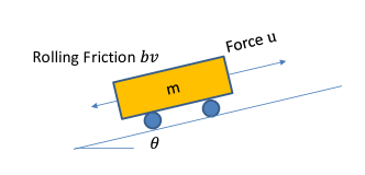
Figure 4: The dynamics of a simplified cruise control system.

Problem description.

Consider a simplified cruise control system shown in Fig. 4. Given a constant reference speed $v_{r}$, the engine tries to maintain the speed of the vehicle to $v_{r}$ by applying an appropriate force $u$. However, in autonomous driving mode, changes in the slope $\theta$ of the road influence the actual vehicle speed $v$. The rolling friction is proportional to the actual speed with a constant coefficient $b$.

Assume the control of the force is implemented by a Proportional-Integral (PI) controller with two constants $k_{p},k_{i}$, i.e., $u=k_{p}(v_{r}-v)+k_{i}\int_{0}^{t}(v_{r}-v(\tau))d\tau$. Also let $\theta$ always have a small value ($-10^{\circ}\leq\theta\leq 10^{\circ}$), so we use $\theta$ in replace of $\sin\theta$. Let $g$ be the gravity constant and $\dot{v}$ be the first derivative of velocity. If the mass of the vehicle is $m$, we have the following equation to describe the system dynamics:

$$m\dot{v}=u-mg\sin\theta-bv\cong[k_{p}(v_{r}-v)+k_{i}\int_{0}^{t}(v_{r}-v(\tau))d\tau]-mg\theta-bv$$ (5)

We rewrite the equations by setting $v$ to $v_{r}+\delta$, where $\delta$ represents the difference between the actual speed and the reference speed. As $v_{r}$ does not change over time, Eq. 5 is rewritten as:

$$m\dot{\delta}=-k_{p}\delta-k_{i}\int_{0}^{t}\delta(\tau)d\tau-mg\theta-b(v_{r}+\delta)$$ (6)

We define the angle of the road $\theta$ to be the input signal, the velocity difference $\delta$ to be the output signal, and the rest to be internal signals. The Bounded-input-bounded-output (BIBO) stability of the system refers to the requirement that for a bounded angle of the slope, the velocity error compared to the reference $v_{r}$ should as well be bounded. To ensure BIBO stability of the system, a designer selects appropriate values for control parameters $k_{p}$ and $k_{i}$. However, the problem is more complicated when the mass of the vehicle is not a fixed system parameter, but rather a parameter that is within a certain bound to reflect the scenario that 1 to 4 passengers of different weights can be seated in the vehicle during operation. Therefore, the task is to find the set of parameters that ensures BIBO stability for all possible values of the mass. It is important to note that the problem is essentially a game-theoretic setting, as the uncontrollability is reflected at runtime by the variation of passenger loads.

Laplace transform and constraint generation.

For the cruise control problem, we apply a Laplace transform to create the model to the frequency domain. For simplicity, we neglect friction and set $b$ to $0$. Then the following formula is the corresponding expression of Eq. 6 in the transferred frequency domain.

$$ms\Delta(s)=-k_{p}\Delta(s)-k_{i}\frac{\Delta(s)}{s}-mg\Theta(s)$$

By rearranging the items in the equation, the transfer function of the system is the following form: $\frac{\Delta(s)}{\Theta(s)}=\frac{-mgs}{ms^{2}+k_{p}s+k_{i}}$. Let the denominator of the transfer function of a continuous-time causal system be $Den(s)$, the set of all controllable constants be $C_{ctrl}$, and the set of all uncontrollable constants be $C_{env}$. Borrowing established results in control theory, BIBO stability is ensured if all roots of the denominator polynomial have negative real parts.

$$\exists c_{1},\ldots,c_{m}\in C_{ctrl}\;\forall e_{1},\ldots,e_{n}\in C_{env},\alpha,\beta\in\mathbb{R}:Den(\alpha+\beta i)=0\rightarrow(\alpha<0)$$

Notice that $Den(\alpha+\beta i)=0$ can be rewritten as a conjunction of two constraints where one constraint covers the real part and the other covers the imaginary part. For the cruise control problem, its corresponding algebraic problem can be formulated as the following: $\exists k_{p},k_{i}\;\forall m,\alpha,\beta:m(\alpha+\beta i)^{2}+k_{p}(\alpha+\beta i)+k_{i}=0\rightarrow(\alpha<0)$. By splitting the real part and the imaginary part, we derive the following formula.

$$\exists k_{p},k_{i}\;\forall m,\alpha,\beta:(m(\alpha^{2}-\beta^{2})+k_{p}\alpha+k_{i}=0\,\wedge\,2m\alpha\beta+k_{p}\beta=0)\rightarrow(\alpha<0)$$

Routh-Hurwitz criterion.

The formulation above does not yield bounds on $\alpha$ and $\beta$. The Routh-Hurwitz criterion [23] from the control domain gives sufficient and necessary conditions for stability to hold in a continuous-time system based on analyzing coefficients of a polynomial $\sum^{n}_{k=1}a_{k}s^{k}$ without considering $\alpha$ and $\beta$. E.g., if the denominator polynomial is $f(s)=a_{4}s^{4}+a_{3}s^{3}+a_{2}s^{2}+a_{1}s+a_{0}$, then for all roots to have negative real parts, all coefficients must be greater than $0$, $a_{3}a_{2}>a_{4}a_{1}$, and $a_{3}a_{2}a_{1}>a_{4}a_{1}^{2}+a_{3}^{2}a_{0}$. The Routh-Hurwitz criterion can be exploited to make EFSMT more efficient.

For the cruise control problem, we have the polynomial $ms^{2}+k_{p}s+k_{i}$ of second degree. Let $m\in[600,1200]$, and $k_{p},k_{i}\in[-100,100]$. We derive the following simple constraint by applying the Routh-Hurwitz criterion:

$$\exists k_{p},k_{i}\in[-100,100]\,\forall m\in[600,1200]:m>0\,\wedge\,k_{p}>0\,\wedge\,k_{i}>0$$ (7)

Therefore, EFSMT returns $k_{p},k_{i}$ by ensuring that they are greater than 0. Often the problem under analysis is described by polynomials of fifth or sixth degree where EFSMT is very useful.

5.4 Certificate Generation for Lyapunov Functions

In BIBO stability analysis, the problem is restricted to linear time-invariant (LTI) systems and the analysis is performed in the frequency domain. Lyapunov analysis targets asymptotic stability of nonlinear systems with analysis on the time domain.

Problem description.

Consider the following scalar nonlinear system:

$$\frac{dx}{dt}=\frac{2}{1+x}-x$$ (8)

An equilibrium point is the point that makes $\frac{dx}{dt}=0$. The above system has an equilibrium point $x=1$, as $\frac{dx}{dt}=\frac{2}{1+1}-1=0$. We are interested in certifying the asymptotic stability of an equilibrium point, i.e., under small disturbances, whether it is possible to move back to the equilibrium point. For example, for an inverted pendulum, the upright position is unstable, as any small disturbance makes the inverted pendulum drop. However, a normal pendulum is stable at its lowest position, as the energy dissipation due to air-friction eventually brings the pendulum back to the low-hanging position.

Lyapunov stability analysis.

To prove stability, we apply Lyapunov analysis, which targets to find an energy-like function $V$ and a radius $r$. It then proves that for all points within the bounding sphere whose center is the equilibrium point and the radius is $r$ (except the center where $V(x)=0$), $V(x)>0$ and $\dot{V}(x)\leq 0$. Intuitively, as $\dot{V}(x)\leq 0$, the energy dispersion ensures that all points within the sphere stay close to the equilibrium point.

For this problem, we first perform the change of axis by setting $z=x-1$. This sets the equilibrium point to $z=0$.

$$\frac{dz}{dt}=\frac{2}{2+z}-z-1$$

The second step is to describe the energy function as templates. Here we use the use $V(z)=az^{2}$, where $a$ is a constant to be synthesized by EFSMT. Then $\dot{V}(z)=\dot{z}z=2az(\frac{2}{2+z}-z-1)=\frac{-2az(z^{2}+3z)}{(2+z)}$. Assume our interest is within $-5\leq z\leq 5$. We can then reduce the problem of Lyapunov stability to the following:

$$\exists a,r\,\forall z\in[-5,5]:(r>0)\wedge((0<|z|<r)\rightarrow(V(z)>0\wedge\dot{V}(z)\leq 0))$$

To process the constraint in EFSMT, we observe that $\dot{V}(z)$ involves division. $\dot{V}(z)\leq 0$ is equal to the constraint $2az(z^{2}+3z)(2+z)\geq 0$. For $V(z)>0$, the condition is to have $a>0$. We then derive the following constraint.

$$\exists a>0,r>0\,\forall z\in[-5,5]:(0<z<r\,\vee\,-r<z<0)\\ \rightarrow 2az(z^{2}+3z)(2+z)=2az^{2}(z+2)(z+3)\geq 0$$ (9)

Constraint strengthening.

Here, we demonstrate the use of constraint strengthening using bitvector theories.

• As we know that when $z=0$, the condition ($\dot{V}(0)=0$) holds, for simplicity we change $(0<z<r\,\vee\,-r<z<0)$ to $-r<z<r$. After strengthening each conjunction, we derive $z+1_{bit}>-r\wedge z-1_{bit}<r$.

• If $2a\geq 0$ then $z^{2}(z+3)(2+z)\geq 0$. We have $z\geq 0$ or $-2\leq z\leq 0$. Strengthening creates $(z-1_{bit}\geq 0)$ or $(z-1_{bit}\geq-2\wedge z+1_{bit}\leq 0)$.

• If $2a<0$ then $z^{2}(z+3)(2+z)\leq 0$. We have $z\leq-3$. Strengthening creates $z+1_{bit}\leq-3$.

The constraint in Eq. 10 is the strengthened condition for using EFSMT with bitvector theories. When setting $1_{bit}$ to be $\frac{1}{32}$, EFSMT returns true with $a=\frac{1024}{32}=32$ and $r=\frac{32}{32}=1$. Therefore, by using the energy function $V(z)=32z^{2}$, with bitvector theories we show that Lyapunov stability is achieved at $x=1$ in a sphere of radius $1$.

$$\exists a,r\in[0,10]_{BV}\,\forall z\in[-10,10]_{BV}:(z+1_{bit}>-r\wedge z-1_{bit}<r)\rightarrow\\ ((2a\geq 0\rightarrow((z-1_{bit}\geq 0)\vee(z-1_{bit}\geq-2\wedge z+1_{bit}\leq 0)))\wedge(2a<0\rightarrow(z+1_{bit}\leq-3)))$$ (10)

Effect of constraint strengthening.

Notice that Lyapnuov stability guarantees that the system remains near the equilibrium point, while asymptotic stability guarantees the convergence toward that point. In this example, due to constraint strengthening, EFSMT can only prove Lyapunov stability ($V(z)>0\wedge\dot{V}(z)\leq 0$) but not asymptotic stability ($V(z)>0\wedge\dot{V}(z)<0$), although it also holds for $a=32,r=1$.

Using JBernstein.

In Eq. 9, when we follow the first step in strengthening to the change $(0<z<r\,\vee\,-r<z<0)$ to $-r<z<r$, the newly generated formula already satisfies the shape in Eq. 4, thereby is solvable with JBernstein (as F-solver) and linear arithmetic (for E-solver). With JBernstein, EFSMT returns true with the same radius $r=1$ but another energy function $V(z)=8z^{2}$.

6 Using EFSMT

The current implementation of EFSMT uses Yices2 SMT. In addition, we have extended JBernstein with the following features: (a) accept constraints with parameterized coefficients (e.g. $3x_{1}+2x_{2}$), (b) programmatically provide an array of assignments (e.g. $(x_{1},x_{2})=(1,1)$), (c) solve constraints where every coefficient is concretized, and (d) programmatically report the results of validity checking. This makes the using of JBernstein into EFSMT possible. Similar to Yices2, EFSMT offers a C API that facilitates users to access basic functionalities and to create their own textual input formats. Fig. 5 demonstrates the usage of the API for the simple constraint

$$\exists x\,\forall y:(0<y<10)\rightarrow(y-2x<7)$$

⬇

1#include<iostream>

2#include<string>

3#include<vector>

4#include"efsmt.h"

5...

6void testExecuteSolver1_LA_LA() {

7

8vector<Variable> existentialVariables;

9vector<Variable> universalVariables;

10vector<expression> assum;

11vector<expression> guar;

12vector<expression> cond;

13

14// Existential variables

15Variable x = { "x", EFSMT_VAR_REAL };

16existentialVariables.push_back(x);

17

18// Universal variables

19Variable y = { "y", EFSMT_VAR_REAL };

20universalVariables.push_back(y);

21

22// Assumption

23assum.push(insertAssignment("y>0","GT","y","0"));

24assum.push(insertAssertion("y>0"));

25assum.push(insertAssignment("y<10","LT","y","10"));

26assum.push(insertAssertion("y<10"));

27

28// Guarantees

29guar.push(insertAssignment("tmp","MUL","2","x"));

30guar.push(insertAssignment("tmp2","SUB","y","tmp"));

31guar.push(insertAssignment("y-2x<7","LT","tmp2","7"));

32guar.push(insertAssertion("y-2x<7"));

33

34// Conditions

35EFSMTProblem prob;

36prob.existentialVariables = existentialVariables;

37prob.universalVariables = universalVariables;

38prob.assumptions = assum;

39prob.guarantees = guar;

40prob.conditions = cond;

41prob.problemType = EFSMT_PROB_LA_LA;

42prob.solverOption = EFSMT_FULL;

43executeEFSMTSolver(prob, EFSMT_SOLVER_YICES2,false);

44}

Figure 5: Encode constraint $\exists x\,\forall y:(0<y<10)\rightarrow(y-2x<7)$ using the API of EFSMT.

Figure 6: A physical model of a wheeled inverted pendulum .

First, we declare two vectors to store existential and universal variables. Line 15 declares variable $x$ in the domain of reals. Line 16 categorizes $x$ as an existential variable. Then we define three vectors assum (stores assumptions in universal variables), cond (stores conditions in existential variables), and guar (the general constraint). Constraints stored in each vector are conjuncted. Therefore, $(\texttt{assum}\rightarrow\texttt{guar})\wedge\texttt{cond}$ forms the specified quantifier-free constraint. Admittedly, all constraints can be described in the guar-vector. The separation is for performance considerations: For example, separating cond from the general constraint allows the F-solver to omit constraints specified in cond. There are two types of actions: insertAssignment() that creates intermediate terms and insertAssertion() that specifies a term which evaluates to either true or false. At line 29, $2\times x$ is created and stored in variable tmp and line 32 creates the ”y-2x<7” constraint added to the guar vector. Line 41 specifies the problem solving type as EFSMT_PROB_LA_LA, meaning that both E-solver and F-solver are handled by linear arithmetic. Line 42 enforces complete search. Line 43 invokes the solver with Yices2 as the underlying engine. The full API specification and documentation is included in the efsmt.h header file.

Performance.

We briefly summarize preliminary results concerning the performance of EFSMT. For nonlinear constraint checking, due to advantages offered by JBernstein, the performance is considerably fast. For example, in the PVS test suite, JBernstein solves problems (in the best case) two to three orders of magnitude faster than existing tools such as QEPCAD [6] and REDLOG [16]. Short query response time makes the counter-example guided approach applicable. For problems with only Boolean variables (2QBF), the introduction of multiple instances (e.g., set $\alpha=2$ or $3$) ameliorates performance nearly linear to the used number (when number is small). Because we do not modify the underlying code structure of Yices2, we are unable to integrate known tricks that are used in 2QBF solving, such as Plaisted-Greenbaum transformation [29]. We have independently implemented another 2QBF solver using SAT4J [25] that utilizes partial assignment and contexts. We compare it with the QBF solver QuBE++ [19] by disabling its preprocessing ability (i.e., to perform simplification and generate formulas with fewer variables) to compare the performance on the core engine. Not surprisingly, as our implementation extends the work in [21] which has demonstrated its superiority over QuBE++, the solver is faster even without our optimization.

Case study: wheeled inverted pendulum.

We outline a concrete example in modeling and parameter synthesis that ensures stability of a wheeled inverted pendulum - a two-wheeled Segway implemented with Lego Mindstorm and RobotC.

Design and Assumptions.

During the design process, two wheels are locked to allow only forward and backward movement. We assume that wheels are always in contact with the ground and experience rolling with no slip. Furthermore, we consider no electrical and mechanical loss. Finally, the inverted pendulum is equipped with a Gyro-meter to measure angular displacement and velocity.

Open system.

The graphical model of the open system with the above assumptions is shown in Fig. 6. By using the Lagrange method (generalized Newton dynamics), we derive the dynamics of the system to the following equation:

$$M_{2}l\ddot{x}\cos\theta+(J_{2}+M_{2}l^{2})\ddot{\theta}-M_{2}gl\sin\theta=0$$

where $J_{1}$ and $J_{2}$ are rotation inertia for the wheel and object (represented as the upper circle), $g$ is the Newtonian gravity constant, $\ddot{x}$ is the second derivative of displacement, and $M_{1}$, $M_{2}$ are masses of the wheel and the object.

Control.

Let $\tau$ be the provided torque, the term we want to control to avoid falling. Then the rotational acceleration generated by the torque on the wheel is given by $\ddot{x}=r\alpha$, where $\alpha=\frac{\tau}{J_{1}}$. Assume that the inverted pendulum is initially placed vertically ($\theta=0$) and will experience only very small disturbance. We apply small-angle approximation to let $\sin\theta\approx\theta$ and $\cos\theta\approx 1$. After simplification, the following equation is generated:

$$M_{2}lr\frac{\tau}{J_{1}}+(J_{2}+M_{2}l^{2})\ddot{\theta}-M_{2}gl\theta=0$$ (11)

From this equation we observe that when no torque is applied ($\tau=0$), state $(\theta,\dot{\theta})=(0,0)$ is an equilibrium point for the inverted pendulum. However, any small displacement (i.e., $\theta\neq 0$) creates $\ddot{\theta}$ and makes the pendulum fall. Let the controller be implemented with Proportional (P) or Proportional-Derivative (PD) controllers. Then we have two unknown parameters $k_{p}$, $k_{i}$ for synthesis. Implementing a PD controller replaces $\tau$ by $k_{p}(\theta-0)+k_{d}\dot{\theta}$.

Synthesis.

In this problem we need to synthesize control parameters $k_{p}$, $k_{d}$ which are represented as existential variables. To prove Laynupov stability, we need to find parameters for the energy function. Let $x_{1}=\theta$ and $x_{2}=\dot{\theta}$. For energy functions, we use templates such as $V=a(x_{1})^{2}+b(x_{2})^{2}$. We use existential variables $\overline{x_{1}},\overline{x_{2}}$ to form the bounding sphere. States $(x_{1},x_{2})$ and environment parameters that need to be tolerated are expressed by universal variables. We also let $M_{2}$, $l$ be universal variables that range within bounded intervals to capture modeling imprecision; we assume that the fluctuation of $M_{2}$ and $l$ are sufficient for capturing the real dynamics of the pendulum shown on the left of Fig. 6. Finally, we pass the following constraint to EFSMT to synthesize control parameters for asymptotic stability.

$$\exists\overline{x_{1}},\overline{x_{2}}>0\,\exists k_{p},k_{d}\,\exists a,b>0\,\forall x_{1},x_{2},M_{2},l:\\ (|x_{1}|<\overline{x_{1}}\,\wedge\,|x_{2}|<\overline{x_{2}})\rightarrow(V(x_{1},x_{2})>0\,\wedge\,\dot{V}(x_{1},x_{2})<0)$$

In both P and PD controllers, EFSMT fails to find a witness for asymptotic stability $\dot{V}(x_{1},x_{2})<0$ with the initial condition $(\theta,\dot{\theta})=(k,0)$ where $k\neq 0$, as these states makes $\dot{V}(x_{1},x_{2})=0$. Therefore, with Lyapunov theorem, the solver can at best prove Lyanupov stability (i.e., $\dot{V}(x_{1},x_{2})\leq 0$). Stronger results, such as Krasovski-Lasalle principle [2], are needed to derive asymptotic stability when $\dot{V}$ is negative semidefinite.

7 Related Work

EFSMT differs from pure theory solvers such as Cylindrical Algebraic Decomposition (CAD) [11] tools (e.g., QEPCAD [6] and REDLOG [16]) or Quantified Boolean Formula (QBF) solvers (e.g., QuBE++ [19]) in that it allows combination of subformulas with variables in different domains into a single constraint problem. From a design perspective, this allows to model control and data manipulation simultaneously (for example, EFSMT can naturally encode the hybrid control problem stated in Section. 5.2). Compared to SMT solvers such as Yices2, Z3 [14], or openSMT [7], EFSMT can analyze more expressive formulas with one quantifier alternation. Furthermore, the nonlinear arithmetic is based on Bernstein polynomials [27] and other assisting techniques (discharging, strengthening) rather than CAD. Admittedly, CAD can solve problems with arbitrary quantifier alternation. However, problems under investigation in EFSMT are more restricted, as we only have one quantifier alternation. Overall, our methodology applies verification techniques (such as CEGAR, abstract interpretation) to guide the process. Our counter-example based approach can be viewed as a technique of CEGAR. The use of two solvers in our solver is borrowed from the technology in the SAT community [28]. It is also an extension from recent results in solving QBF via abstraction-refinement [21]. However, our method is combined with infeasibility test (that uses widening) to fully utilize the capability of two separate solvers. In addition, our proposed optimization techniques (e.g., the effect of partial assignment) are never considered by these works.

For reduction problems presented in this work, safety orchestration of component-based systems using priorities was first proposed by Cheng et al. [8]. The algorithm is based on a heuristic that performs bug finding and fixing. We extend the work by using a template-based reduction that allows to easily encode architectural constraints and other artifacts in distributed execution (e.g., knowledge). Safety control for timed systems first appeared in the work by Maler, Pnueli and Sifakis [26]. Tools such as UPPAAL-Tiga [4] allow to synthesize strategies for timed games. EFSMT uses a template-based approach, meaning that the synthesized safety-invariant is fixed in its shape. Therefore, the goal is not to find a controller that maintains maximal behavior. However, as demonstrated in the example (Section 5.2), constraint encoding allows synthesis on a wider application not restricted to timed systems. For stability control [2], Lyapunov functions are in general difficult to find. Our reduction to EFSMT searches for feasible parameters when the shape of the Lyapunov function is conjectured. It can be used as a complementary technique to known methods in control domain that systematically searches for candidate templates (e.g., sum-of-square methods [30]). Finally, for the analysis in the frequency domain (Section 5.3), graphical or numerical methods (such as Bode diagrams [23]) are often used to decide the position of a root in the complex plane. These methods are applied when parameters are fixed. Other graphical methods such as Nyquist plot [23] are used for deciding parameterized behavior. Algebraic or symbolic methods that extend Routh-Horwitz criterion include the well-known Kharitonov’s theorem [5] which allows to detect stability for polynomials with parameters of bounded range. In other words, if values of design parameters are provided by the $\exists$-solver, an implementation of Kharitonov’s theorem can also act as a $\forall$-checker for BIBO stability. Gulwani and Tiwari verify hybrid systems [20] with exists-forall quantified first-order fragment of propositional combinations over constraints, and the technology is based on a quantifier elimination procedure. As demonstrated in our example, we use the technique to do synthesis of hybrid control systems, and our method is based on CEGAR. In addition, we show a richer set of problems that can be encoded within the framework such as Lyanupov certificate synthesis. We also show that progress can be ensured without another quantifier alternation by carefully trimming the synthesized strategy structure to be priorities.

8 Conclusion

EFSMT extends propositional SMT formulas with one top-level exists-forall quantification. We have demonstrated, by means of reducing a variety of design problems, including the stability of control systems and orchestration of system components, that EFSMT is an adequate logical framework for the design and the analysis of cyber-physical systems. The EFSMT fragment of first-order logic is expressive enough to allow strategy finding for safety games, while strategies for other properties can be derived by either restricting the structure (e.g., the use of priorities to ensure progress) or game transformation (e.g., bounded synthesis [32] that transforms LTL synthesis to safety games via behavioral restrictions). We also propose an optimized verification procedure for solving EFSMT based on state-of-the-practice SMT solvers and the use of Bernstein polynomials for solving nonlinear arithmetic constraints. Although we have restricted ourselves to arithmetic constraints, the approach is general in that rich combinations of theories, as supported by SMT solvers, can readily be incorporated. Future extensions of the EFSMT proof procedure are mainly concerned with performance and usability enhancements, but also with completeness.

References

- [1] R. Alur and D. Dill. A theory of timed automata. Theoretical Computer Science, 126(2):183–235, 1994.
- [2] K. Astrom and R. Murray. Feedback Systems: an introduction for scientists and engineers. Princeton university press, 2008.
- [3] A. Basu, M. Bozga, and J. Sifakis. Modeling heterogeneous real-time components in BIP. In SEFM, pages 3–12. IEEE, 2006.
- [4] G. Behrmann, A. Cougnard, A. David, E. Fleury, K. Larsen, and D. Lime. UPPAAL-Tiga: Time for playing games! In CAV, volume 4590 of LNCS, pages 121–125. Springer, 2007.
- [5] S. Bhattacharyya, H. Chapellat, and L. Keel. Robust control. Prentice-Hall, New Jersey, 1995.
- [6] C. W. Brown. QEPCAD-B: a program for computing with semi-algebraic sets using CADs. SIGSAM Bull., 37(4):97–108, Dec. 2003.
- [7] R. Bruttomesso, E. Pek, N. Sharygina, and A. Tsitovich. The openSMT solver. In TACAS, volume 6015 of LNCS, pages 150–153. Springer, 2010.
- [8] C.-H. Cheng, S. Bensalem, B. Jobstmann, R.-J. Yan, A. Knoll, and H. Ruess. Model construction and priority synthesis for simple interaction systems. In NFM, volume 6617 of LNCS, pages 466–471. Springer, 2011.
- [9] C.-H. Cheng, H. Ruess, and N. Shankar. JBernstein: A validity checker for generalized polynomial constraints. In CAV, 2013, to appear.
- [10] A. Cimatti. Beyond boolean SAT: satisfiability modulo theories. In WODES, pages 68–73. IEEE, 2008.
- [11] G. Collins and H. Hong. Partial cylindrical algebraic decomposition for quantifier elimination. Journal of Symbolic Computation, 12(3):299–328, 1991.
- [12] P. Cousot and R. Cousot. Abstract interpretation: a unified lattice model for static analysis of programs by construction or approximation of fixpoints. In POPL, pages 238-252. ACM, 1977
- [13] S. Cruanes, G. Hamon, S. Owre and N. Shankar. Tool Integration with the Evidential Tool Bus In VMCAI, volume 7737 of LNCS, pages 275–294. Springer, 2013.
- [14] L. De Moura and N. Bjørner. Z3: An efficient SMT solver. In TACAS, volume 4963 of LNCS, pages 337–340. Springer, 2008.
- [15] L. De Moura, H. Rueß, and M. Sorea Lazy Theorem Proving for Bounded Model Checking over Infinite Domains In CADE, volume 2392 of LNCS, pages 438–455. Springer, 2002.
- [16] A. Dolzmann and T. Sturm. Redlog: computer algebra meets computer logic. SIGSAM Bull., 31(2):2–9, June 1997.
- [17] B. Dutertre and L. De Moura. The Yices SMT solver. Tool paper available at http://yices.csl.sri.com/tool-paper.pdf, 2:2, 2006.
- [18] M. Ernst, T. Millstein, and D. Weld. Automatic SAT-compilation of planning problems. In IJCAI, pages 1169–1177. Morgan Kaufmann, 1997.
- [19] E. Giunchiglia, M. Narizzano, and A. Tacchella. QuBE++: An efficient qbf solver. In FMCAD, volume 3312 of LNCS, pages 201–213. Springer, 2004.
- [20] S. Gulwani and A. Tiwali. Constraint-based Approach for Analysis of Hybrid Systems. In CAV, volume 5123 of LNCS, pages 190–203. Springer, 2008.
- [21] M. Janota and J. Marques-Silva. Abstraction-based algorithm for 2QBF. In SAT, volume 6695 of LNCS, pages 230–244. Springer, 2004.
- [22] H. Kautz and B. Selman. Unifying SAT-based and graph-based planning. In IJCAI, volume 1, page 318–325. Morgan Kaufmann, 1999.
- [23] B. Kuo and M. Golnaraghi. Automatic control systems, 4th Edition. John Wiley & Sons, 2008.
- [24] S. Lahiri, S. Qadeer, and Z. Rakamarić. Static and precise detection of concurrency errors in systems code using SMT solvers. In CAV, volume 5643 of LNCS, pages 509–524. Springer, 2009.
- [25] D. Le Berre and A. Parrain. The SAT4J library, release 2.2. Journal on Satisfiability, Boolean Modeling and Computation, Volume 7 (2010), system description, pages 59-64.
- [26] O. Maler, A. Pnueli, and J. Sifakis. On the synthesis of discrete controllers for timed systems. In STACS, volume 900 of LNCS, pages 229–242. Springer, 1995.
- [27] C. Muñoz and A. Narkawicz. Formalization of a representation of Bernstein polynomials and applications to global optimization. Journal of Automated Reasoning, 2012. Accepted for publication.
- [28] D. P. Ranjan, D. Tang, and S. Malik A Comparative Study of 2QBF Algorithms. In SAT, 2004.
- [29] D.A. Plaisted and S. Greenbaum. A structure-preserving clause form translation. Journal of Symbolic Computing 2(3), 293–304 (1986)
- [30] S. Prajna, A. Papachristodoulou, and P. A. Parrilo. SOSTOOLS: Sum of squares optimization toolbox for MATLAB, Tool paper available at http://www.cds.caltech.edu/sostools., 2002
- [31] J. Rushby. An evidential tool bus. In Formal Methods and Software Engineering, volume 3785 of LNCS, pages 36–36. Springer, 2005.
- [32] S. Schewe and B. Finkbeiner Bounded Synthesis. In ATVA, volume 4762 of LNCS, pages 474–488. Springer, 2007.
- [33] M. Sorea. Bounded Model Checking for Timed Automata, In ENTCS, 2002, Vol. 68(5), http://www.elsevier.com/locate/entcs/volume68.html
- [34] W. Steiner. An evaluation of SMT-based schedule synthesis for time-triggered multi-hop networks. In RTSS, pages 375–384. IEEE, 2010.
- [35] M. Yuan, X. He, and Z. Gu. Hardware/software partitioning and static task scheduling on runtime reconfigurable fpgas using a SMT solver. In RTAS, pages 295–304. IEEE, 2008.