Spinful fermionic ladders at incommensurate filling: Phase diagram, local perturbations, and ionic potentials

Abstract

We study the effect of external potential on transport properties of the fermionic two-leg ladder model. The response of the system to a local perturbation is strongly dependent on the ground state properties of the system and especially on the dominant correlations. We categorise all phases and transitions in the model (for incommensurate filling) and introduce “hopping-driven transitions” that the system undergoes as the inter-chain hopping is increased from zero. We also describe the response of the system to an ionic potential. The physics of this effect is similar to that of the single impurity, except that the ionic potential can affect the bulk properties of the system and in particular induce true long range order.

1 Introduction

The wonderful world of electrons confined to move in one dimension has fascinated physicists for more than fifty years. Since the pioneering work of Tomonaga [1] and Luttinger [2], powerful theoretical methods have been devised to treat interacting one-dimensional (1D) systems [3, 4, 5, 6], culminating in establishing the concept of the Tomonaga-Luttinger (TL) liquid [6, 7] (see for a review [8, 9]). The distinctive feature of the TL liquid is that the elementary excitations have nothing to do with free electrons, but rather consist of plasmon-like collective modes. Moreover, various perturbations, such as backscattering or Umklapp processes, can lead to the development of a strong-coupling regime where spectral gaps are dynamically generated [10, 11, 12] without spontaneous breakdown of any continuous symmetry [13].

For a long time, beautiful one-dimensional models mainly remained in the theoretical domain. However, due to recent technological advances, quantum wires have become experimentally realizable [14, 15], and one-dimensional physics is undergoing a renaissance. TL-liquid effects have been observed in carbon nanotubes [16, 17, 18, 19], and cleaved edge [20, 21] and V-groove [22] semiconductor quantum wires.

Though much experimental effort goes into making quantum wires as clean as possible, any real system inevitably contains some degree of disorder. The traditional approach to disorder in solids builds on the approximation of nearly free electrons. At a certain concentration of impurities the system undergoes an Anderson localization transition [23, 24]. This one-particle description of disorder has been realized in all possible dimensions – in particular, it was established that in one-dimensional disordered systems electrons are always localized [25].

Going beyond the free electron limit one must study the interplay of disorder and electron-electron interactions – one of central topics in modern condensed matter physics. If disorder strength is insufficient to reach the Anderson transition, the electrons remain mobile and one finds interaction corrections to physical observables [26]. On the other hand, when free electrons are localized by disorder, then the electron-electron interaction is not expected to change the insulating nature of the ground state [27]. This can not be the whole story in 1D systems, however; here interactions may dramatically change the nature of the ground state and therefore should never be considered as a small perturbation.

In a seminal paper [28], Kane and Fisher have shown that, due to strong correlation effects, transport properties of the TL liquid can dramatically change even in the presence of a single impurity. While a clean TL liquid is an ideal conductor, a single impurity, no matter how weak, completely reflects the charge carriers driving the zero-temperature conductance to zero in the physical case of repulsive bulk interactions. This may also be understood [29] as an extreme limit of the Altshuler-Aronov corrections [26]; the reduced dimensionality enhances the effect such that it may no longer be considered a correction.

The result of Kane and Fisher is specific to purely 1D models where a strongly renormalized impurity potential effectively splits the chain into two disconnected pieces. Conversely, if a single impurity is added to a two- or three-dimensional system, then, no matter how strong, such perturbation will have no effect whatsoever on global observable properties. Exactly how one can interpolate between one- and two-dimensional (2D) behavior (i.e. between the TL and Fermi liquids) is still an open question, despite considerable theoretical effort [30, 31, 32]. Instead, one can consider a simpler situation where only a small number of 1D systems are coupled to form a ladder-like lattice.

The simplest ladder model is that of a two-leg ladder. The extensive research in this field [33, 34, 37, 39, 43, 46, 47, 49, 53, 54, 36, 35, 38, 41, 40, 44, 45, 50, 55, 48, 51, 52, 56, 42] is motivated in part by purely theoretical reasons (e.g. the crossover between the 1D and 2D), but also by a plethora of experimental realizations. Many solids are structurally made up of weakly coupled ladders [57], which leaves a wide temperature range within which the properties are dominated by one-dimensional physics. Of particular relevance are the metallic ladder compounds which include the “telephone number” compound Sr_14-xCa_xCu₂₄O₄₁ [58, 59] and PrBa₂Cu₄O₈ [60] as well as members of the cuprate family Sr_n-1Cu_n+1O_2n after hole doping [61]; for a review of such compounds see Ref. [62]. It was also suggested that such physics may be seen in the (fluctuating) stripe ordered phase in certain cuprate high-temperature superconductors [63]. More recently, the development of nanotechnology has reached the point where systems manufactured in the laboratory can be “tailored” to resemble microscopic models of interest. Double-chain nanostructures can be manufactured [20] while multi-sub-band quantum wires [64, 65] have a theoretical low-energy description equivalent to that of ladders [66]. Similarly, metallic single wall carbon nanotubes [67] have a low energy description equivalent to that of a two-leg ladder [68, 70, 69], the two channels (legs) originating from the valley degeneracy of graphene. The ladder geometry can also be created in optical lattices in cold atoms experiments [71, 72, 73].

Taking the viewpoint that ladder models may serve as an intermediate step between purely 1D and 2D systems, we ask a natural question: does the dramatic response of interacting 1D systems to a local potential extend onto the ladder structures as well? In a recent publication [74], we addressed this question in the context of the spinless ladder (e.g. in the model where the particles hopping on the ladder are spin polarized electrons). We found that in the case where the bulk interaction is repulsive, the effect of a generic local potential is described by the Kane-Fisher scenario leading to vanishing conductance, $G\rightarrow 0$ at $T\rightarrow 0$. Physically, this result follows from the fact that the external potential couples to the local density-wave order parameter which determines leading dynamical correlations in the ground state of the system.

While this result might have been expected, it has a rather surprising corollary: if the impurity potential is tuned to the form that does not couple to the dominant order parameter, then the density wave does not get pinned by the impurity and the ladder exhibits ideal conductance (at $T=0$). Thus, contrary to a naive expectation, a potential applied symmetrically at the two opposite sites of a given rung of the ladder remains transparent [74].

In this paper we extend our analysis to the more realistic case where the charge carriers in the system are real electrons. Our strategy remains the same as above: to describe transport properties of the system, we need to (i) identify the nature of the ground state of the model, (ii) determine which local operator acquires a non-zero expectation value in a given ground state, and, finally, (iii) establish whether the external perturbation couples to the dominant order parameter. Throughout the paper we consider a generic, incommensurate filling.

The problem of a single impurity is essentially that of $2k_{F}$ backscattering at a single point in the one-dimensional structure. One can extend this to the case where such a backscattering occurs uniformly throughout the entire ladder, a perturbation known as an ionic potential. The theoretical attraction of this problem is apparent: the structure of the gaps and correlations in the ground state of the unperturbed ladder and the ionic crystal are not necessarily the same – and therefore the path from one to the other may show rich physics with one or more quantum phase transition as happens in the interplay between the Mott insulator and band insulator in single chains [75]. Beyond the theoretical interest, there are also a number of natural experimental realizations of such an ionic potential. The telephone number compound [58, 59] consists of both ladders and chains with incommensurate lattice spacings. Hence the chains provide an ionic potential for the ladders within the same system. By varying the doping, the periodicity of this potential may be tuned to the Fermi level. Similarly, ordered monolayers of atoms adsorbed onto the surface of carbon nanotubes [76] act as an ionic potential on the electrons within the nanotube. Furthermore, such ionic potentials may be seen as intermediate between single impurities and true disordered systems [77]. In fact, within cold-atom systems in an optical lattice, the addition of a second incommensurate optical lattice is often used to mimic disorder [78, 79], the combined bichromatic lattice having only quasi-periodicity.

The first step in the above program, i.e. finding the ground state correlations of the ladder model, is well studied [33, 34, 37, 39, 43, 46, 47, 49, 53, 54, 36, 35, 38, 41, 40, 44, 45, 50, 55, 48, 51, 52, 56, 42], with all possible ground states [49] and transitions between them [53] discussed in the literature. However, the scattered nature and sheer number of relevant publications in the field presents a certain challenge when one wants to find the answer to a seemingly straightforward question: given a set of values of the microscopic parameters of the model Hamiltonian, what is the ground state of the system and what is the nature of dominant correlations? Having been unable to identify a single source, where this question could be answered for arbitrary values of the model parameters, we decided that this paper would be incomplete without an overview of the phase diagram of the ladder model in the absence of the perturbation. In particular, previous works have mostly concentrated on the limits when inter-chain hopping is either large or small; to our knowledge, how one of these limits evolves into the other has not yet been studied. We therefore spend some time on this question before studying the effects of the perturbations.

The structure of the paper is as follows: in Sec. 2 we introduce the model, review previous literature and summarize our main results. The main body of the paper then provides the formalism from which these results are obtained. In Section 3 we present the phase diagram for the model of two capacitively coupled chains, followed by the discussion in Section 4 of the phase diagram of the two-leg ladder, where the inter-chain hopping is sufficiently strong. Comparing the phase diagrams in Sections 3 and 4, we notice significant differences between the two. Therefore, in Section 5 we introduce a concept of a “hopping-driven phase transition” and describe the evolution of the ground state of the model as the inter-chain hopping parameter $t_{\perp}$ is increased from zero.

Having identified the necessary properties of the model in the absence of external perturbations, we turn to the central issue of this paper, namely the effect of a local perturbation, which we discuss in Section 6. In Section 7 we argue that the analysis of Section 6 can be extended to the case of the ionic potential. We conclude the paper with a summary and outlook. Technical details are relegated to Appendices.

2 The model and summary of results

In this section, we define the ladder model and external perturbations that we will consider in this paper. We then present a historic summary of what is already known about the ladder model before summarizing the results that will be derived in the remainder of this paper.

2.1 The Hamiltonian of the ladder model

We consider a model Hamiltonian consisting of the single-particle part ${\cal H}_{0}$ and the interaction terms ${\cal H}_{\text{int}}$

$${\cal H}={\cal H}_{0}+{\cal H}_{\text{int}}.$$ (1a)

The single-particle part of the Hamiltonian $${\cal H}_{0}$$ represents a nearest-neighbor tight-binding model

$${\cal H}_{0}=-\frac{t_{\parallel}}{2}\sum_{im\sigma}c_{i,m,\sigma}^{\dagger}c_{i+1,m,\sigma}-t_{\perp}\sum_{i\sigma}c_{i,1,\sigma}^{\dagger}c_{i,2,\sigma}+H.c,$$ (1b)

while $${\cal H}_{\text{int}}$$ contains an on-site Hubbard term as well as in-chain and inter-chain nearest-neighbor density-density interactions :

$${\cal H}_{\text{int}}=U\sum_{i,m}n_{i,m,\uparrow}n_{i,m,\downarrow}+V_{\|}\sum_{i,m,\sigma,\sigma^{\prime}}n_{i,m,\sigma}n_{i+1,m,\sigma^{\prime}}+V_{\perp}\sum_{i,\sigma,\sigma^{\prime}}n_{i,1,\sigma}n_{i,2,\sigma^{\prime}}.$$ (1c)

In above formulas $c_{i,m,\sigma}$ is the annihilation operator of an electron with the spin projection $\sigma=\uparrow(\downarrow)$ localized at the site $i$ of the chain $m=1,2$, (hereafter this set of fermionic operators will be referred to as the chain basis), $n_{im\sigma}=c^{\dagger}_{i,m,\sigma}c_{i,m,\sigma}$ are the occupation number operators, and $t_{\|}$ and $t_{\perp}$ are the intra- and inter-chain hopping amplitudes, respectively. This Hamiltonian is illustrated schematically in Fig. 1.

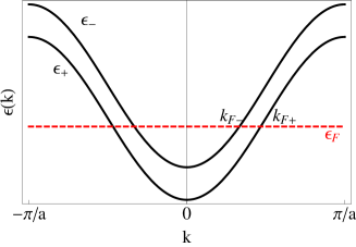
Figure 1: (a) The geometry and interactions of the two-leg ladder. The legs consist of tight binding chains with hopping integral $t_{\parallel}$, and on-site ($U$) and nearest-neighbor ($V_{\|}$) interaction. The legs are then coupled via inter-chain hopping $t_{\perp}$ and interaction $V_{\perp}$. (b) Dispersion of the two-leg ladder. We consider the case of an incommensurate filling such that the Fermi level goes through four Fermi points $\pm k_{F+}$ and $\pm k_{F-}$.

The kinetic part of the Hamiltonian has a spectrum consisting of two cosine bands

$$\epsilon_{\pm}(k)=-t_{\|}\cos(ka)\mp t_{\perp}.$$ (2)

where $a$ is the longitudinal lattice spacing. In this paper, we analyze main features of this model at incommensurate filling factors such that the Fermi level goes through four Fermi points, as illustrated in Fig. 1. Consequently Umklapp processes play no role in our analysis and therefore the unperturbed model always remains in the metallic regime: while certain collective modes may acquire a gap, the total charge mode always remains gapless.

2.2 External perturbations

The main goal of this paper is to describe the effect of external perturbations on the ground state and transport properties of the ladder model (1). We will restrict our discussion to perturbations that couple to the carrier density in the system, either locally, in which case the perturbation potential describes a single impurity, or globally which is the case of an ionic potential.

2.2.1 Local perturbation (single impurity)

A local external perturbation respecting the SU(2) spin symmetry can be described by the general expression

$${\cal H}_{\rm imp}=\sum_{b}\lambda_{b}\sum_{m,m^{\prime},\sigma}c^{\dagger}_{i=0,m,\sigma}\tau^{b}_{mm^{\prime}}c_{i=0,m^{\prime},\sigma},$$ (3)

where $b=0,x,y,z$ and $\tau^{b}$ are the Pauli matrices acting in chain space (with $\tau^{0}$ being the identity). Here the $b=0$ and $b=z$ terms are local analogs of the two types of charge density waves in the ladder, CDW⁺ and CDW^-, illustrated in Fig. 3 below (more details on the local operators in the model are given in D). The $b=x$ term describes a local fluctuation in the inter-chain hopping amplitude $t_{\perp}$ and $b=y$ corresponds to a local (orbital) magnetic field.

A usual scattering center on the chain $m=1$ is described by Eq. (3) with $\lambda_{0}=\lambda_{z}$, while an impurity on the chain $m=2$ is described by $\lambda_{0}=-\lambda_{z}$; in both cases the off-diagonal terms $\lambda_{x}=\lambda_{y}=0$. For clarity, we eliminate these off-diagonal terms in (3) for the bulk of the manuscript; generalization of our results to the case $\lambda_{x},\lambda_{y}\neq 0$ is straightforward.

2.2.2 Ionic potential

We now extend the local potential (3) periodically to the whole ladder to obtain a bulk perturbation:

$${\cal H}_{\rm ion}=\sum_{b}\lambda_{b}\sum_{i,m,m^{\prime},\sigma}\cos(Kai)c^{\dagger}_{i,m,\sigma}\tau^{b}_{mm^{\prime}}c_{i,m^{\prime},\sigma}.$$ (4)

If the modulation wave vector $K$ is commensurate with the density of particles , $K=2k_{F}$, then the $b=0$ and $b=z$ terms are proportional to the local operators that serve as order parameters for CDW⁺ and CDW^-, respectively. Such a perturbation is known as an ionic potential.

If the energy scale associated with the ionic potential is the largest in the system, then the particles will arrange themselves at the minima of the cosine potential, with the energy levels forming bands as in the usual Bloch theory. The case of commensurability $K=2k_{F}$ then corresponds to the lowest band being completely filled. The system in this limit is a band insulator. In the absence of ${\cal H}_{\rm ion}$, the ground state of the ladder model (1) is a conducting state, but typically with a spin gap. The question then is whether one can go smoothly between these two limits, or whether there is necessarily a quantum phase transition at some finite value of $\lambda_{b}$.

While at first sight the physics of the ionic potential and that of the local impurity may seem completely different, we will show they are related. The analysis of the local impurity is dominated by the $2k_{F}$ backscattering spawned from the perturbation (3). The physical effect this term has is then determined by how it is affected by the correlated ground state of the unperturbed system. Similarly, the important contribution of the ionic-potential (4) is the $2k_{F}$ backscattering – this is affected by the ground state in the same way as the local impurity, however because it occurs in the bulk rather than just at a point it may now have a back effect on this ground state, potentially giving rise to the aforementioned quantum phase transitions.

2.3 Summary of previous work on Ladder models

To set the scene for the present work, we briefly review the existing literature on ladder models. Initially, the studies were motivated by the question: what happens when TL liquids are coupled? Earlier works were mainly focused on density-wave structures in arrays of chains coupled by interaction only (see e.g. [80, 81] and references therein). In the beginning of the nineties, however, the main attention was shifted towards the possible role of inter-chain hopping. Most notably, the involved issues were the relevance of the single-particle hopping [82, 83, 84, 31] which may lead to a confinement phase, along with the importance of the generated pair-hopping [85]. This was studied in detail for the case without spin [36], where it was seen that the confinement phase manifests itself in a commensurate-incommensurate (C-IC) transition at which the Fermi-points belonging to the two bands become split. Furthermore, the generated pair-hopping terms gave rise to various phases with quasi-long-range order, including the previously elusive orbital antiferromagnetic phase, also known in the literature as the staggered flux or $d$-density wave phase.

When a similar study was conducted for the spinful ladder [35, 38, 37, 41], something quite different was discovered. It appeared that, for generic interactions, there was a spin gap in the spectrum, in strong contrast to the single chain case. Furthermore, it was demonstrated that even for repulsive interactions dominant correlations in the system may be of the superconducting type. These exciting properties led to a renewed interest in the ladder models. It was soon understood that the spin gap is present for all ladders with an even number of legs, while those with an odd number of legs, including the single chain, show gapless spin excitations [40, 57]. This is closely related to the existence of a gap in antiferromagnetic spin chains with an integer spin and its absence for chains with a half-integer spin [86]. This implies that the ground state of the system may be a Haldane spin-liquid [42], a topological phase of matter showing Majorana-fermion edge states [87]. On top of this, in half-filled ladders with a ground state of a spin-gapped Mott insulator, already weak doping causes dominance of superconducting fluctuations – the fact going in a remarkable parallel with the two-dimensional cuprate high-temperature superconductors [62]. It was therefore believed that one could gain insight into the properties of high-$T_{c}$ materials by studying ladder toy models. Indeed, by coupling many ladders together into a 3D structure, one finds a true phase transition to a strongly correlated superconductor [88, 90, 89, 91].

A lot of effort was therefore expended establishing the complete phase diagram of the two-leg ladder model. Initially, the work concentrated on the Hubbard model [44, 45, 43]; later studies included more generic interactions, and, in addition to superconducting correlations, density wave and orbital antiferromagnetic phases were found [49, 50, 55]. This gave a complete picture of the phase diagram [49] in the regime where the Fermi-points are split by the inter-chain hopping term. Studies of the confinement regime and consequent C-IC transitions were limited to densities close to half-filling, where the charge (Mott) gap was the catalyst for confinement [48].

The analytic studies of the ladders are mostly based on a weak coupling RG approach and bosonization. This is backed up by numerics which is particularly useful for tracing the phase diagram at intermediate and large bare couplings. However, the presence of gaps means that even weak bare couplings flow to a strong coupling fixed point which cannot be reliably described using perturbative RG methods. The quest to describe the strong-coupling phases led to various parallel developments in the theory of ladders. One of the most important is the phenomenon of dynamical symmetry enhancement [46]. This occurs when the low-energy fixed point of the theory has a higher symmetry than that of the underlying lattice model. In Ref. [46], it was shown that, in the case of a weakly interacting two-leg ladder, the low-energy effective theory has an O(6)$\times$ U(1) symmetry for the generic incommensurate case; at half filling it is further enhanced to O(8). Technically this means that the weak-coupling RG flow converges towards high-symmetry rays [92] (perturbations that break the high symmetry down to the bare lattice symmetry are irrelevant in the RG sense). This high-symmetry fixed point is often integrable [47] implying that the strong-coupling regime may be described non-perturbatively at the solvable point, while treating irrelevant symmetry-breaking operators as weak perturbations.

Another concept that is important for undersrtanding of the strong-coupling phases of the model is duality [93]. There is not one but many high-symmetry rays in the parameter space. These correspond to different ground states of the system and are related to each other by some non-local transformation. Some of the dualities may even be exact on the lattice [51], but in the most general form they are a property emerging in the low-energy limit. Now we can interpret the phase transitions between different ground states as located at the separatrices between the RG basins of attraction of two of these high-symmetry rays in parameter space. These represent self-dual points of the corresponding duality transformations [93].

The final important tool developed to understand the strong-coupling phases is the refermionization approach [42]. The advantage of the refermionized theory over abelian bosonization is that the underlying symmetry of the model remains explicit. This fact simplifies identification of various criticalities [52].

Such an approach was used in Ref. [53] in order to describe a complete picture of the phase diagram previously propounded in [49]. The phase transitions were all classified into the universality classes Z₂ (Ising), U(1) (Berezinskii-Kosterlitz-Thouless) and that of the SU(2)₂ Wess-Zumino-Novikov-Witten model. The elementary excitations and excitation spectrum throughout the phase diagram were also calculated. However, the consideration was limited to the region where the Fermi points in the two bands were split, i.e. the system was not in a confined phase. Further works have extended this study to the case when spin and charge velocities may be very different [56]. Experimentally relevant properties such as the NMR relaxation rate have also been calculated [94, 95, 96].

Important further developments address the role of disorder[97, 98, 99]. One of the main conclusions reached is that for any repulsive interactions (or weak attractive ones), the disorder is always relevant driving the system to a localized phase. Some other works worthy of note are Ref. [66], where disorder and some transport properties of a two-subband quantum wire were also studied; Ref. [100] where weak localization in the two-leg ladder was studied; and the recent publication [101] which looks at some aspects of the two-leg ladder in an ionic potential.

2.4 Summary of present results

For the benefit of the reader not interested in technical details, we summarize our results here. Our principal results are three-fold. Firstly, we introduce the notion of hopping-driven phase transitions, in-particular those relating to confinement. Secondly, we establish the effect of the single impurity on the ground state and transport properties of the system. Finally, we extend our results on the single-impurity problem to the effect of the ionic potential.

These results rely on the precise knowledge of the phase diagram of the model including the nature of the phase transitions. Although all of the phases of the ladder model are already known, we have included a detailed discussion of the phase diagram in order to make the paper self-contained.

2.4.1 Hopping-driven phase transitions

Microscopic Hamiltonians describing electronic systems, including strongly correlated ones, often contain separate single-particle (e.g. tight-binding or kinetic) and interaction terms (our Hamiltonian (1) is no exception). In a typical experiment, one may vary the carrier density (e.g. by applying external electro-static potentials), temperature, pressure, etc., and try to modify the effective strength of electron-electron interaction. At the same time, the parameters describing the bare single-particle spectrum are determined by the crystal properties of the material and are assumed to remain constant in the course of the measurements (a notable exception is the case of pressure-induced structural phase transitions [102]).

Recently there has been renewed interest in the Hubbard-type models due to the rapid advances in the experimental techniques related to optically trapped cold atoms [103]. In such measurements, almost any parameter of the optical lattice can be controlled by tuning the laser fileds that create the optical traps. Thus it is conceivable to study the evolution of the observable properties of the system with the change in tunneling amplitudes, and in particular, the interchain hopping parameter $t_{\perp}$.

The fact that such evolution should go through critical regions associated with quantum phase transitions can be seen by comparing the phase diagrams of the ladder model (1) in the two cases of vanishing and sufficiently large inter-chain hopping shown in Figs. 4 and 5, respectively. The most obvious differences between the two is the absence of the CDW⁺ and TL liquid phases in Fig. 5. At the same time, the superconducting (SC) phases and the orbital anti-ferromagnet (OAF) can only appear in the presence of $t_{\perp}$.

Our primary technical tool is the perturbative (“one-loop”) renormalization group (RG). The RG equations are formulated on the basis of the effective low-energy field theory, which in turn relies upon the details of the single-particle spectrum [8, 9]. The latter undergoes significant changes as the inter-chain hopping is introduced. Consequently, the RG equations for $t_{\perp}=0$ and large $t_{\perp}$ (given by Eqs. (15) and (26), respectively) are rather different. However in the representation used in Eq. (26), known as the band-basis, the inter-chain hopping parameter $t_{\perp}$ itself is not part of the RG equations, as it couples to a topological current of the theory. As soon as $t_{\perp}$ is changed, the RG flow has to be re-calculated. Thus, in order to describe the evolution of the system as $t_{\perp}$ increases from zero, we use a two-cut-off scaling procedure, explained in Section 4.2. One may use an alternative approach and derive the RG equations in the chain basis. Then the operator that couples to $t_{\perp}$ is a vertex operator with a nonzero conformal spin and subject to renormalization. We outline how this looks in section 3.5, but do not develop this further, since this alternative procedure does not allow us to follow the phase diagram to the large $t_{\perp}$ limit.

Numerical integration of the RG equations within the two-cut-off scaling procedure results in the $t_{\perp}-V_{\perp}$ phase diagram (see Fig. 6), that illustrates the hopping-driven phase transitions. Note, that the TL liquid phase that exists for $t_{\perp}=0$ is unstable with respect to an infinitesimal addition of inter-chain hopping – as soon as $t_{\perp}$ is switched on, the system forms the $OAF$ phase.

In the most physical case of repulsive interaction and under an additional assumption $U\gg V_{\|}$ the system undergoes the first-order transition between the CDW^- phase at low $t_{\perp}$ and SC^d phase at higher $t_{\perp}$. However, if $U<V_{\|}$, then the system remains in the CDW^- phase and there is no phase transition. This result agrees with the naive expectation of the CDW^- phase being compatible with the inter-chain hopping, based on the cartoon description of this phase shown in Fig. 3.

On the contrary, the CDW⁺ phase (also illustrated in Fig. 3) appears to be incompatible with $t_{\perp}$. As $t_{\perp}$ is increased past some low but non-zero value, the system undergoes an Ising-type (Z₂) transition to one of the SC phases (depending on the value of $V_{\perp}$). Moreover in a narrow range of $V_{\perp}$, the system exhibits a second transition from the SC^s phase to the CDW^- phase. This transition nominally belongs to the SU(2)₂ universality class and corresponds to the change of sign of the dynamically generated mass of the spin-triplet sector in the re-fermionised formulation of the effective low energy field theory, however marginal interaction terms are expected to drive it weakly first order.

2.4.2 The effect of a local perturbation

As in the Kane-Fisher problem [28], there are generically two possibilities for the response of the system to the local impurity. Either the impurity is a relevant perturbation completely reflecting the electrons and driving the system towards insulating behavior

$$G(T)\propto T^{\gamma^{\prime}},$$ (5)

or the perturbation is irrelevant and one sees only a small correction to the perfect conductance

$$G(T)=\frac{4e^{2}}{h}-CT^{\gamma}.$$ (6)

Here the positive exponents $\gamma$ and $\gamma^{\prime}$ are nonuniversal and depend on the interactions in the system.

For a single chain, realization of a particular scenario depends on the Luttinger parameter $K_{c}$. Roughly speaking, for repulsive interactions, $K_{c}<1$, the insulating case (5) holds, while for attractive interactions, $K_{c}>1$, the system remains a conductor (6). In Ref. [74], we have shown that the resulting conductance of a spinless ladder depends not only on the interactions but also on the local structure of the impurity potential. For repulsive interactions when the system is in the CDW^- phase, this results in the curious phenomenon: a single impurity on one of the legs of the ladder drives the system to an insulating regime with the low-temperature conductance given by (5), whereas a symmetric impurity on both legs keeps the ladder transparent for transport.

The explanation for this result was quite simple [74]: in the former case, the local perturbation couples directly to the local order parameter operator that describes dominant correlations of the bulk system (see above Section 2.4.1 above). In the latter case, there is no direct coupling – the impurity looks locally like the CDW⁺ while the correlators of these are short ranged in the bulk CDW^- phase.

The concept of whether the local perturbation couples directly to the order parameter or not also plays an important role in the present case of the spinful two-leg ladder. There is an important difference however between the present case and the spinless ladder previously studied. Within the perturbative RG approach to impurities in the spinful ladder it turns out that not only first order but also second order scattering terms are relevant when the bulk interactions are repulsive, $K_{c}^{+}<1$. As we will show, this implies that no local potential is transparent at $K_{c}^{+}<1$; the insulating behavior (5) holds irrespective of the structure of the impurity. The importance of the local structure of the impurity in the spinful ladder lies in the fact that the exponent $\gamma^{\prime}$ does strongly depend on this structure. In this sense, the metal-insulator transition of the spinless case transforms to a strong crossover in the present model. To be more specific, in the bulk CDW^- phase and for $K_{c}^{+}=1-\delta$, one obtains $\gamma^{\prime}\approx 6$ for the case of a single impurity on one chain and $\gamma^{\prime}=2\delta$ for the symmetric impurity. A summary of the results for the exponent $\gamma^{\prime}$ for both cases as well as the exponent $\gamma$ for the metallic side (which may occur for attractive interactions) is given in Table 2.

Another difference to the spinless case is that the order parameter for a large portion of the phase diagram (see Figs. 4, 5 and 6) is superconducting. In particular, for repulsive interactions one typically has either the CDW^- phase or the $SC^{d}$ phase, depending on whether the interchain interaction or the interchain hopping is dominant. In the latter case, no local density perturbation couples directly to the order parameter and so the structure of the perturbation becomes unimportant. On the other hand, this strongly correlated (quasi-long range order) superconducting state nevertheless becomes insulating (for $K_{c}^{+}<1$) when any impurity is added.

All above considerations apply to energies (temperatures) less than the dynamically generated gaps in the system, the results being technically obtained by integrating out the high-energy gapped degrees of freedom leaving an effective single-channel model for the current-carrying gapless mode. Close to any of the phase transition lines (discussed in Section 2.4.1 above) however, one observes the softening of further modes, leaving a wide temperature range between these new close-to-critical modes and the remaining gapped ones. The properties of the system then depends crucially on which phase transition we are talking about, and therefore there is a rich variety of possibilities. Thus transport at or near one of the quantum critical lines is governed by modified power laws; which are summarized in Table 3. For $K_{c}^{+}<1$, we see that the behavior is again that of an insulator, given by (5). Finally, even if the temperature is bigger than all of the gaps, the system is still an insulator for $K_{c}^{+}<1$; in this case, the general result is given by (56).

2.4.3 Ionic potential

As with the local perturbation, we may express an ionic potential commensurate with the carrier density in terms of the same operators used to describe the dominant correlations of the unperturbed system. When the energy scale of the added ionic potential is much larger than the dynamically generated gaps, the dominant correlations in the system are clearly going to be of the same type as the potential we have explicitly added. If the unperturbed ground state of the system showed different correlations, then the system must evolve from one sort of correlation to the other as a function of the applied perturbation $\lambda_{b}$ in Hamiltonian (4).

This evolution may happen in one of two ways – it may be smooth; or it may undergo certain quantum-phase transitions en route. Examples of such phase transitions are known in similar situations in the literature – for example, the SU(2)₁ transition in dimerized spin ladders [104, 105] or zig-zag carbon-nanotubes [106]; or the two transitions between the Mott insulator and the band insulator in a half-filled single chain in an ionic potential [75].

Our aim in this work is to categorize the transitions that may or may not take place when an ionic potential is added to the doped (incommensurate) two-leg ladder. Clearly, this depends on both the ground state of the unperturbed system, as well as the type of ionic potential added. To be specific, we consider ionic potentials coupling to the local density (of either CDW⁺ or CDW^- types) added to a system with any of the five possible ground states discussed in this work. To avoid too many cases, we also limit ourselves to the situation when $K_{c}^{+}<2$.

In all cases we consider, we find that the first effect of adding the ionic potential, $\lambda_{b}\neq 0$, is that the previously critical total charge mode $\phi_{c}^{+}$ becomes gapped. In other words, the system immediately exhibits true long range order and becomes an insulator. This doesn’t contradict the Hohenberg-Mermin-Wagner theorem [13] for there is no spontaneous symmetry breaking – the external ionic potential explicitly breaks the translational symmetry.

We then proceed to identify any quantum phase transitions that may take place as $\lambda_{b}$ becomes larger, see Table 4. As expected, we find that if the ionic potential has the same structure as the already existing correlations, then there is no possibility of a transition. We also find that if the ground state is in one of the superconducting phases, the evolution is smooth. In all other cases however, we find there is some critical $\lambda_{b}^{*}$ at which the system becomes critical; the universality class for each case is listed in Table 4.

3 Capacitively coupled chains

Consider a situation where two individual quantum wires are placed close enough to each other such that the Coulomb interaction between electrons in different wires is strong enough and, at the same time, there is no direct contact between the wires preventing the electrons from tunneling from one wire into another. This system can be described by the ladder Hamiltonian (1b), (1c) in the absence of inter-chain hopping

$$t_{\perp}=0,$$

and was first studied in Ref. [33]. In this case, the Fermi momenta for all four channels remain the same, and the single-particle Hamiltonian (1b) is diagonal at the outset. Therefore it is natural to discuss the case of $t_{\perp}=0$ using the original chain basis. We first briefly review the case of two completely decoupled chains, before adding the inter-chain interaction $V_{\perp}$ and analyzing the effect such a term has on the ground state of the system.

3.1 Two independent chains

In the absence of interchain hopping the two chains are connected only by the interaction $V_{\perp}$. If one sets $V_{\perp}=0$, then the model reduces to two copies of the 1D extended Hubbard model. Its bosonized form is well-known [8] (see A for details and notations). The most prominent feature of this model is spin-charge separation. In particular, the effective low-energy theory (88) contains two decoupled sectors describing collective charge and spin degrees of freedom.

The case of two independent chains is rather trivial – we now have two copies of charge and spin fields (87), which we denote as $\phi_{m,c}$ and $\phi_{m,s}$ ($m=1,2$ is the chain index). Thus for $V_{\perp}=t_{\perp}=0$ the model Hamiltonian can be written in the form (88a) where the charge sector contains two copies of the Gaussian model

$${\cal H}_{c}=\frac{v_{F}}{2}\sum_{m}\left[\Pi_{m,c}(x)^{2}+\left(1-\frac{h_{c}}{\pi v_{F}}\right)\left[\partial_{x}\phi_{m,c}(x)\right]^{2}\right],$$ (7a)

and the spin sector – two copies of the sine-Gordon model

$${\cal H}_{s}=\frac{v_{F}}{2}\sum_{m}\left[\Pi_{m,s}(x)^{2}+\left(1-\frac{h_{s}}{\pi v_{F}}\right)\left[\partial_{x}\phi_{m,s}(x)\right]^{2}\right]+\frac{h_{s}}{2(\pi\alpha)^{2}}\sum_{m}\cos\sqrt{8\pi}\phi_{m,s}(x).$$ (7b)

As the chains are identical, the interaction parameters are independent of the chain index $m$. In terms of the original lattice coupling constants they are given by

$$h_{c}=-aU-2aV_{\parallel}\left[2-\cos(2k_{F}a)\right],$$

$$h_{s}=aU+2aV_{\parallel}\cos(2k_{F}a).$$ (8)

Notice that the same constant $h_{s}$ appears in two different terms in Eq. (7b). This is a consequence of SU(2) symmetry. In fact, Eqs. (7) is more general than the original lattice model, and one may consider the decoupled legs of the ladder parameterized via $h_{c}$ and $h_{s}$ rather than $U$ and $V_{\|}$.

At $h_{s}>0$ the perturbation is marginally irrelevant, the model flows to weak coupling, and the spectrum remains gapless. At $h_{s}<0$ the perturbation is relevant, the model flows to strong coupling, and the spin sector acquires a spectral gap. Note that for fillings between $1/4<n<1/2$, $\cos(2k_{F}a)<0$, so both cases can occur even for purely repulsive bare interactions (in fact the upper limit of fillings is $3/4$ but for the sake of concreteness, we will always deal with the case of less than half filling), depending on whether $U$ or $V$ is dominant. These two different phases are schematically illustrated in Fig. 2.

Figure 2: Cartoon depictions of the two possible phases of the extended Hubbard model with repulsive interactions. In a), the on-site interaction is dominant ($h_{s}>0$), in this case the Néel order is quasi-long range and the spectrum remains gapless. In b) the nearest-neighbor interaction is dominant ($h_{s}<0)$, in this case the singlets don’t break any symmetry and the spectrum acquires a finite spin gap. In these cartoons (as well as other similar depictions below), the circles do not represent lattice sites (we are incommensurate), but instead indicate fluctuating charge positions an average of $\pi a/2k_{F}$ apart.

It is easy to understand within a strong-coupling picture (see e.g. Fig. 2) why the interactions $U$ and $V$ are in competition with each other for fillings between $1/4$ and $1/2$. The on-site interaction $U$ makes double occupancy energetically unfavourable – which for this range of fillings means particles must be placed in nearest neighbor positions. Such neighboring particles feel an exchange interaction; which means that in this phase the dominant correlations are those of the spin-density wave type. The interaction $V$ favours opposite configurations, where particles don’t sit in neighboring positions; and therefore there must be some double occupancy. In this case, the dominant correlations are of the charge-density wave type, while the doubly occupied singlets lead to the presence of a spin-gap. The transition at the point $U=-2V\cos(2k_{F}a)$ (i.e. $h_{s}=0$) is exactly of the BKT type.

3.2 Inter-chain interaction

Consider now the interchain interaction $V_{\perp}$ described by the last term in Eq. (1c). Its bosonized version can be obtained using representation (81) for the fermion density (with all bosonic fields supplied with the additional chain index). The result is a sum of two terms

$$\sum_{\sigma\sigma^{\prime}}n_{i,1,\sigma}n_{i,2,\sigma^{\prime}}\rightarrow S_{\rm fs}+S_{\rm bs}.$$

The first term is the interchain forward scattering

$$S_{\rm fs}=\frac{1}{\pi}\partial_{x}\phi_{1,c}\partial_{x}\phi_{2,c}.$$

The second term is the interchain backscattering similar to Eq. (85d):

$$S_{\rm bs}=\cos\sqrt{2\pi}\left[\phi_{1,c}-\phi_{2,c}\right]\cos\sqrt{2\pi}\left[\phi_{1,s}+\phi_{2,s}\right]$$

$$\quad\quad\quad+\cos\sqrt{2\pi}\left[\phi_{1,c}-\phi_{2,c}\right]\cos\sqrt{2\pi}\left[\phi_{1,s}-\phi_{2,s}\right].$$

Now we rearrange the bosonic fields into four linear combinations that correspond to the total and relative charge, as well as total and relative spin:

$$\phi_{c(s)}^{\pm}=\frac{\phi_{1,c(s)}\pm\phi_{2,c(s)}}{\sqrt{2}}.$$ (9)

This transformation simplifies the interchain backscattering terms and at the same time diagonalizes the quadratic part of the Hamiltonian, which now contains four copies of the Gaussian model:

$${\cal H}_{0}=\frac{v_{F}}{2}\sum_{\begin{subarray}{c}\mu=c,s\\ \nu=\pm\end{subarray}}\left[\Pi_{\mu}^{\nu}(x)^{2}+\left(1-\frac{g_{\mu}^{\nu}}{\pi v_{F}}\right)\left[\partial_{x}\phi_{\mu}^{\nu}(x)\right]^{2}\right].$$ (10a)

The remaining part of the bosonized Hamiltonian contains the inter- and intra-chain backscattering terms

$${\cal H}_{\rm bs}=\frac{g_{1}}{(\pi\alpha)^{2}}\cos\sqrt{4\pi}\phi_{s}^{+}\,\cos\sqrt{4\pi}\phi_{s}^{-}$$

$$\quad\quad+\frac{g_{2}}{(\pi\alpha)^{2}}\cos\sqrt{4\pi}\phi_{c}^{-}\left[\cos\sqrt{4\pi}\phi_{s}^{+}+\cos\sqrt{4\pi}\phi_{s}^{-}\right].$$ (10b)

Backscattering terms (10b) couple the relative charge mode ($\phi_{c}^{-}$) to the total ($\phi_{s}^{+}$) and relative ($\phi_{s}^{-}$) spin modes. The corresponding coupling constants in the Hamiltonian (10) may be parameterized as

$$g_{c}^{-}=h_{c}+h_{\perp},\quad g_{s}^{\pm}=g_{1}=h_{s},\quad g_{2}=h_{\perp},$$ (11a)

where

$$h_{\perp}=aV_{\perp}$$ (11b)

while $$h_{c} h_{s}$$ and are defined in Eqs.(8).

The first two parameters in Eq. (11b) coincide with Eq. (8) reflecting the fact, that for $V_{\perp}=0$ the Hamiltonian (10) describes two uncoupled chains [c.f. Eqs. (7)]. In fact, this parameterization is valid for any two spinful TL-liquids coupled via a density-density interaction, where $h_{c}$ and $h_{s}$ parametrize the chains, and $h_{\perp}$ the interchain coupling. We will therefore retain this trio $h_{c},h_{s},h_{\perp}$ throughout the paper as a convenient way to parameterise the phase diagram of the model.

The total charge mode ($\phi_{c}^{+}$) is decoupled from the rest of the spectrum and hence describes a TL liquid with the Luttinger parameter

$$K_{c}^{+}\approx 1+\frac{g_{c}^{+}}{2\pi v_{F}}.$$ (12)

As this algebraic relation only holds for weak interactions $|g_{c}|\ll 1$, while the TL liquid concept is much more general, it is therefore appropriate to think of the Luttinger parameter $K_{c}^{+}$ as the fourth independent parameter of the ladder. There is another reason to consider $K_{c}^{+}$ independently. Much of our analysis of the Hamiltonian (10) will be based on the renormalization group, where the parameters $h$ will be allowed to flow. Clearly however, no renormalization occurs in the decoupled $\phi_{c}^{+}$ sector which is described by the Gaussian model.

3.3 Refermionized form of the spin sector and symmetries of the model

While the bosonized representation (10) is extremely convenient for a renormalization group analysis, the representation in terms of four scalar bosonic fields obscures the symmetries of the model, particularly in the spin sector where we would expect at least that the SU(2) symmetry is still present, which is not at all apparent in (10). For this reason, we give another representation of the Hamiltonian here, in which the spin sector is re-fermionized. The physical idea behind this technique ultimately goes back to the seminal works by S. Coleman [107] and Itzykson and Zuber [108] in which the equivalence between the sine-Gordon model at the decoupling point ($\beta^{2}=4\pi$), a free massive Dirac fermion, and a pair of noncritical two-dimensional Ising models was established. According to this correspondence the spin sector of the ladder model (1) is equivalent to four weakly coupled quantum Ising chains [108]. The latter can be represented in terms of Majorana fermions [42, 8, 109]. While ultimately, this is just another way of writing the same Hamiltonian, we will see that in the Majorana representation the symmetries of the Hamiltonian are made explicit.

We now introduce four Majorana fermion fields $\xi^{i}_{R(L)}$ to replace the two bosonic spin fields $\phi_{s}^{\pm}$ according to the re-fermionization rules in (91). The Hamiltonian is split up into a kinetic (Gaussian) part and interaction (non-linear) terms,

$${\cal H}={\cal H}_{k}+{\cal H}_{\mathrm{int}},$$ (13a)

which are grouped slightly differently as compared to the fully bosonized case. The kinetic part still includes two Gaussian models for the bosonized charge modes $$\phi^{\pm}_{c} g^{\pm}_{c}$$ with the forward scattering amplitudes explicitly included (see Eq. (10a)), and four massless Majorana fields for the spin modes

$${\cal H}_{k}={\cal H}_{0}\left[\phi_{c}^{+}\right]+{\cal H}_{0}\left[\phi_{c}^{-}\right]+\frac{iv_{s}}{2}\sum_{a=1,2,3,0}\left(\xi^{a}_{L}\partial_{x}\xi^{a}_{L}-\xi^{a}_{R}\partial_{x}\xi^{a}_{R}\right),$$ (13b)

Marginal interaction in the spin sector, parametrized by $$g_{1,2} {\cal H}_{\mathrm{int}}$$, is included in :

$${\cal H}_{\mathrm{int}}=-g_{1}\left(\sum_{a=0}^{3}\xi^{a}_{R}\xi^{a}_{L}\right)^{2}+\frac{ig_{2}}{\pi\alpha}\cos\sqrt{4\pi}\phi_{c}^{-}\sum_{a=0}^{3}\xi^{a}_{R}\xi^{a}_{L},$$ (13c)

There are four independent coupling constants: two of them describe forward scattering in the charge sectors ($g_{c}^{+}$ and $g_{c}^{-}$), and two more describe the spin sectors ($g_{1}$ and $g_{2}$), the bare values being given by Eq. (11) as before. In the absence of the interchain hopping the spin symmetry of the ladder model is that of two decoupled chains: SU(2) $\times$ SU(2) $\approx$ O(4); this is unbroken by an interchain density-density interaction. This is why the Hamiltonian contains only O(4) invariants: $(\sum_{a=0}^{3}\xi^{a}_{R}\xi^{a}_{L})^{2}$ which originates from the intra-chain interaction, as well as the mixed term $\cos\sqrt{4\pi}\phi_{c}^{-}\sum_{a=0}^{3}\xi^{a}_{R}\xi^{a}_{L}$. When interchain hopping processes are allowed, we will see that they generate interchain exchange terms which reduce the spin symmetry from SU(2)$\times$ SU(2) to a single SU(2). As we will see in section 3.5, the O(4) symmetry present in the four Majorana fields will split into a spin-triplet mode described by $\xi^{i}$ with $i=1,2,3$ and a spin-singlet degree of freedom described by the remaining $i=0$ fermion.

3.4 Phase diagram

We now proceed to construct the phase diagram of the model of capacitively coupled chains described by Hamiltonian (1) with $t_{\perp}=0$. We will do this carefully using renormalization group methods in the following, but to begin with let us consider a simple strong coupling picture in the atomic limit. If the interchain interaction is weak, then a good reference point is the state of each individual chain. The single-chain model is described in detail in A and illustrated in Fig. 2.

Let us first suppose that $V_{\|}>U$ (or more precisely, $h_{s}<0$). Then each chain exhibits quasi-long-range order of the CDW type as illustrated in Fig. 2b. When such chains are coupled by interchain interaction $V_{\perp}$, it is clear that all potential energy terms may be minimized by forming density waves on both changes with a relative phase of $0$ for attractive interchain interaction and $\pi$ for the repulsive case. Such states are known as CDW⁺ and CDW^- respectively, and are illustrated in Fig. 3.

In the opposite case when $V_{\|}<U$ ($h_{s}>0$) and the dominant correlations in the uncoupled chains are SDW rather than CDW, the situation is less obvious as there is now competition between the different interaction terms. In fact, the SDW state in the single chain is quite delicate – as the SU(2) symmetry prevents the appearance of a spin-gap in this state. It will therefore turn out that the SDW is unstable to arbitrarily small interchain interaction – the resulting state being either of the CDW^± states mentioned previously, or remaining a TL liquid with no dynamically acquired gaps. In order to analyze this, we will now study more closely the structure of the order parameters.

Figure 3: Cartoon depiction of the (a) CDW⁺ phase and (b) CDW^- phase of the ladder model. The circles represent fluctuating charge positions an average of $k_{F}^{-1}$ apart.

3.4.1 Structure of order parameters and semi-classical analysis

The general form of the local density operators for the spinful ladder is given in D. At present, we are interested in the charge density wave (CDW^±) phases. The corresponding order parameters describe the staggered (oscillating) components of the total and relative charge density operators

$$CDW^{+}\leftarrow\sum_{\sigma}\left(c^{\dagger}_{1\sigma}c_{1\sigma}+c^{\dagger}_{2\sigma}c_{2\sigma}\right),\quad CDW^{-}\leftarrow\sum_{\sigma}\left(c^{\dagger}_{1\sigma}c_{1\sigma}-c^{\dagger}_{2\sigma}c_{2\sigma}\right),$$

and in the bosonic representation are given by

$${\cal O}_{CDW^{+}} \sim e^{-i\sqrt{\pi}\phi_{c}^{+}}\left[\sin\sqrt{\pi}\phi_{c}^{-}\sin\sqrt{\pi}\phi_{s}^{+}\sin\sqrt{\pi}\phi_{s}^{-}-i\cos\sqrt{\pi}\phi_{c}^{-}\cos\sqrt{\pi}\phi_{s}^{+}\cos\sqrt{\pi}\phi_{s}^{-}\right],$$

$${\cal O}_{CDW^{-}} \sim-e^{-i\sqrt{\pi}\phi_{c}^{+}}\left[\sin\sqrt{\pi}\phi_{c}^{-}\cos\sqrt{\pi}\phi_{s}^{+}\cos\sqrt{\pi}\phi_{s}^{-}-i\cos\sqrt{\pi}\phi_{c}^{-}\sin\sqrt{\pi}\phi_{s}^{+}\sin\sqrt{\pi}\phi_{s}^{-}\right].$$ (14)

Notice that the bosonized form of each local operator has a multiplicative structure involving the fields in each of the four sectors of the theory

$${\cal O}=\sum{\cal O}_{c^{+}}{\cal O}_{c^{-}}{\cal O}_{s^{+}}{\cal O}_{s^{-}},$$

and as such, $\langle{\cal O}\rangle=0$ because the gapless and decoupled total charge sector always has $\langle{\cal O}_{c^{+}}\rangle\neq 0$. In other words there is no true long-range order in the system, which is a direct consequence of the Hohenberg-Mermin-Wagner theorem [13]. On the other hand, the notion of quasi-long-range order of the type ${\cal O}$ assumes a situation when the correlator $\langle{\cal O}(r){\cal O}(0)\rangle$ displays the slowest (among all others) power-law decay. This is what is also called algebraic order. Then we say that the dominant correlations are those of the operator ${\cal O}$. There may be other order parameters with power-low asymptotics but they decay faster; the remaining order parameters decay exponentially with a finite correlation length.

We also notice that each operator ${\cal O}$ has a structure of a product of cosines and sines of the fields added to another product with the cosines and sines reversed. The origin of this construct is consistent with the expression Eq. (10b) for the backscattering Hamiltonian. While the latter is invariant under the transformation $\sqrt{4\pi}\phi_{a}\rightarrow\sqrt{4\pi}\phi_{a}+\pi$ , the operators $\cos\sqrt{\pi}\phi_{a}$ and $\sin\sqrt{\pi}\phi_{a}$ get interchanged in all sectors simultaneously. In order to demonstrate this point, we perform a semi-classical analysis of the Hamiltonian (10b) by evaluating the field configurations that minimize the energy. Let us first suppose that $g_{1}<0$ (i.e. $h_{s}<0$ so that each chain forms a CDW). Then to minimize the potential energy Eq. (10b), one locks the fields $\phi_{s}^{\pm}$ either at the set of points $\phi_{s}^{+}=n\sqrt{\pi}$, $\phi_{s}^{-}=m\sqrt{\pi}$; or the set of points $\phi_{s}^{+}=(n+1/2)\sqrt{\pi}$, $\phi_{s}^{+}=(m+1/2)\sqrt{\pi}$ for integers $n,m$. In view of the symmetry above, let us pick the first set of points, for which $\cos\sqrt{4\pi}\phi_{s}^{+}=\cos\sqrt{4\pi}\phi_{s}^{-}=1$. Now consider the role of the inter-layer interaction, i.e. the $g_{2}$ term in Eq. (10b). If $g_{2}<0$, then $\cos\sqrt{4\pi}\phi_{c}^{-}$ also wants to take the value $+1$. If, on the other hand, $g_{2}>0$ then the opposite value $\cos\sqrt{4\pi}\phi_{c}^{-}=-1$ is preferred. Thus for $g_{1}<0$ both back-scattering terms in Eq. (10b) may be minimized simultaneously.

To understand the resulting phases of the system we turn to the order parameters. If both back-scattering coupling terms are negative, then the three fields $\phi_{c}^{-}$, $\phi_{s}^{+}$, and $\phi_{s}^{-}$ are locked at e.g. $0$. Consider now the operator ${\cal O}_{0}$. The product $\cos\sqrt{\pi}\phi_{c}^{-}\cos\sqrt{\pi}\phi_{s}^{+}\cos\sqrt{\pi}\phi_{s}^{-}$ now acquires an expectation value and the correlation function

$$\langle{\cal O}_{0}(x){\cal O}_{0}(0)\rangle\sim\left[\langle\cos\sqrt{\pi}\phi_{c}^{-}\cos\sqrt{\pi}\phi_{s}^{+}\cos\sqrt{\pi}\phi_{s}^{-}\rangle\right]^{2}\langle e^{-i\sqrt{\pi}\phi_{c}^{+}(x)}e^{-i\sqrt{\pi}\phi_{c}^{+}(0)}\rangle\sim\frac{1}{|x|^{\gamma}},$$

will exhibit an algebraic decay with the critical exponent $\gamma=K_{c}^{+}/4$ contributed by the gapless modes of the total charge sector. All other operators, for example ${\cal O}_{z}$ involve either the sines of the above three fields or their dual fields. Therefore the correlation functions of those operators will decay exponentially with a finite correlation length

$$\langle{\cal O}_{z}(x){\cal O}_{z}(0)\rangle\sim e^{-|x|/\xi}.$$

Thus for $g_{1},g_{2}<0$ the dominant correlation is of the CDW⁺ type and hence we refer to this phase as CDW⁺. If $g_{1}<0,g_{2}>0$, then the situation is just the opposite, and the phase is CDW^-, in agreement with the strong coupling atomic limit previously expounded. This situation is similar to the spinless case [54]: if the dominant order within each chain is CDW-like, then when they are brought together a repulsive inter-chain interaction will lock the CDWs with a relative phase $\pi$ while an attractive inter-chain interaction will lock them with relative phase $0$.

Now we turn to the case $g_{1}>0$, where the dominant correlations on the individual chains (in the absence of inter-chain coupling) are of the SDW type. In this case, it is clear that one cannot simultaneously minimize both the $g_{1}$ and the $g_{2}$ terms in the back-scattering Hamiltonian, (10b). Naïvely one might expect a transition between the SDW state (minimizing $g_{1}$) at $g_{1}>2|g_{2}|$ to the CDW state which minimizes the $g_{2}$ term at $g_{1}<2|g_{2}|$. However, such an analysis is too simplistic. In fact, the SDW that would semi-classically minimize the $g_{1}$ term at $g_{1}>0$ is critical (unlike the case $g_{1}<0$) and is thus very sensitive to perturbations. Therefore for $g_{1}>0$ a more rigorous analysis is required.

3.4.2 RG equations in the chain basis and phase diagram

To obtain the phase diagram of the model of two capacitively coupled chains (10), we now employ the renormalization group technique. Apart from the total charge sector which is completely decoupled from the rest of the spectrum, the model contains three independent coupling constants (11). It turns out to be instructive to express the RG equations in terms of the parameters $h_{j}$ given in (11b), remembering that $h_{c}$ and $h_{s}$ parameterise the intra-chain interactions, while $h_{\perp}$ is the strength of inter-chain interaction. The RG equations then take the form

$$\frac{\partial h_{c}}{\partial l} =\frac{h_{\perp}}{2}\left(h_{c}+3h_{s}-3h_{\perp}\right),$$

$$\frac{\partial h_{s}}{\partial l} =-h_{s}^{2}-h_{\perp}^{2},$$

$$\frac{\partial h_{\perp}}{\partial l} =-\frac{h_{\perp}}{2}\left(h_{c}+3h_{s}+h_{\perp}\right),$$ (15)

with the initial values given in Eq. (11b).

It is immediately clear that the plane $h_{\perp}=0$ is invariant, i.e. if there is no initial inter-chain coupling, none is generated under the RG flow, and the model is equivalent to two decoupled copies of the one-dimensional chain. On this plane the equations (15) reduce to the SU(2) BKT equation $\frac{\partial h_{s}}{\partial l}=-h_{s}^{2}$, which describes the physics of the spin sector of the extended Hubbard model (88f), discussed in Appendix A.

It is also clear that there is a line of weak-coupling fixed points

$$h_{s}=0,\quad h_{\perp}=0,$$

where $h_{c}$ may remain arbitrary. At these fixed points all sectors of the theory are Luttinger liquids. The RG possesses also strong coupling fixed points

$$h_{s}\to-\infty,\quad h_{\perp}\to\pm\infty.$$

These strong coupling fixed points correspond exactly to the scenario where the bosonic fields are locked at the minima of the cosine potentials as analysed above. Therefore this is a phase where all sectors except total charge are gapped with the dominant order being of the CDW type. For $h_{\perp}>0$ this is CDW^-, while for $h_{\perp}<0$ it is CDW⁺. By following the RG flow as a function of bare parameters, we can therefore determine the phase diagram of the model.

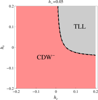
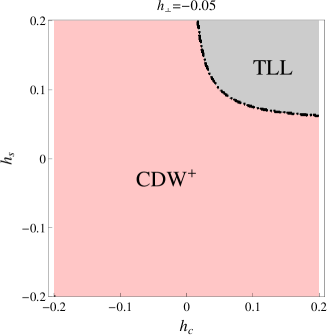
Figure 4: The phase diagram of the system of two capacitively coupled chains for fixed inter-chain interaction (left panel corresponds to $h_{\perp}=0.05$, right panel to $h_{\perp}=-0.05$). Here CDW⁺ and CDW^- are the charge-density waves illustrated in Figs. 3 and TLL stands for the Tomonaga-Luttinger liquid.

In fact, the boundary between the weak- and strong-coupling phases may be determined analytically. As demonstrated in E, the RG possesses an invariant plane

$$\quad h_{s}(h_{\perp}+h_{c})=h_{\perp}^{2}.$$ (16)

which is in fact exactly the phase boundary between the basin of attraction of the strong and weak coupling fixed points. The phase diagram can thus be conveniently parameterised as

$$\quad h_{s}(h_{\perp}+h_{c})>h_{\perp}^{2} : \mathrm{Weak\ coupling-TLL}$$

$$h_{\perp}>0,\quad h_{s}(h_{\perp}+h_{c})<h_{\perp}^{2} : \mathrm{Strong\ coupling-CDW}^{-}$$

$$h_{\perp}<0,\quad h_{s}(h_{\perp}+h_{c})<h_{\perp}^{2} : \mathrm{Strong\ coupling-CDW}^{+}$$ (17)

This resulting phase diagram of the system of two capacitively coupled chains is illustrated in Fig. 4.

We see therefore that even in the case that $h_{s}>0$ and the dominant correlations on the individual chains before they are coupled was SDW and not CDW, the interchain coupling may lead to a CDW state being formed. We note however that in this case, the resulting dynamically acquired gap is much smaller than in the case when the bare $h_{s}<0$ and there was no competition between the different interaction terms.

3.5 Interchain hopping term in the chain basis

Practical calculations are often performed using a particular set of basis operators. In principle, physical results have to be independent of the choice of the basis. On the other hand, this choice does affect technical complexity of the calculations, which can be greatly reduced by choosing an appropriate basis.

In the problem of capacitively coupled chains, the choice of the chain basis (i.e. the set of fermionic operators $c_{i,m,\sigma}$) appears to be most physical. This way one can trace how the Luttinger correlations on each chain interplay with each other when the inter-chain coupling is added to the problem. But once the inter-chain hopping is taken into account (see e.g. [39]), the situation becomes less transparent. Indeed, after bosonization in the chain basis, the inter-chain hopping operator becomes non-local. The origin of this issue can be traced back to the single-particle spectrum of the model, shown in Fig. 1: now that the spectrum contains two individual branches, it is not immediately clear why the bosonization procedure in the vicinity of the single-chain Fermi points is still justified. Instead, it seems natural to rotate the basis from the original fermionic operators $c_{i,m,\sigma}$ to their bonding and anti-bonding combinations that diagonalize the single-particle Hamiltonian (1b). This will be done in the next Section.

Moreover, one can use the above rotated (or band) basis also in the absence of $t_{\perp}$ without incurring significant technical difficulties (albeit at the expence of physical clarity), since in this case the spectrum remains invariant under any unitary rotation of the fermionic basis. But while it is possible to study the whole range of values of $t_{\perp}$ using only the band basis (see discussion of the two-cutoff RG scheme in Section 4.3), it seems reasonable to review several aspects of the role of the inter-chain hopping in the chain basis, where it can be treated perturbatively.

In the second order in small $t_{\perp}$, one finds (in the presence of interactions) coherent processes [82, 83, 85] that foretell much of the physics that will be derived more formally in the next Section. Firstly, there are pair hopping terms, which – if they are the most relevant operators – give rise to dominant superconducting fluctuations. For example in the regime where the un-coupled chains had a spin gap (thus suppressing single-electron tunneling), singlet pairs may hop between the chains, leading to strong s-wave superconducting correlations.

Secondly, inter-chain hopping affects the renornalization of the interaction coupling constants in the model, which results in dynamical generation of the inter-chain exchange (see Footnote 1). Without going into details, the main result of such a term on the low energy effective Hamiltonian is best seen in the refermionized form, where the marginal interaction in the spin-sector previously written in (13c) is modified to become

$${\cal H}_{\mathrm{int}}=-g_{1,t}\left(\sum_{a=1}^{3}\xi^{a}_{R}\xi^{a}_{L}\right)^{2}-g_{1,s}\xi^{0}_{R}\xi^{0}_{L}\sum_{a=1}^{3}\xi^{a}_{R}\xi^{a}_{L}+\frac{i}{\pi\alpha}\cos\sqrt{4\pi}\phi_{c}^{-}\left(g_{2,s}\xi^{0}_{R}\xi^{0}_{L}+g_{2,t}\sum_{a=0}^{3}\xi^{a}_{R}\xi^{a}_{L}\right).$$ (18)

The interchain exchange splits the previously seen O(4) symmetry down to O(3)$\times$Z₂, corresponding to a spin singlet mode (labelled by $a=0$), and a spin-triplet mode (labelled by $a=1,2,3$). Physically, the most important part of ${\cal H}_{\rm int}$ to focus on is the $g_{2}$ terms, which – if relevant – roughly speaking provide the Majorana Fermions with mass (see Section 5.1 for details of the mechanism of Majorana mass generation). The single parameter $g_{2}$ has now split into two parts $g_{2,s}\sim a(V_{\perp}+J_{\perp})$ and $g_{2,t}\sim a(V_{\perp}-J_{\perp})$. If $g_{2,s}$ and $g_{2,t}$ are the same sign, then the singlet and triplet modes are split, but other than this the CDW correlations are fundamentally no different than in the case $J_{\perp}=0$. On the other hand, if the (dynamically generated) inter-chain exchange $J_{\perp}$ is larger than the inter-chain interaction $V_{\perp}$, then $g_{1,s}$ and $g_{1,t}$ will have opposite signs. In this case, the CDW correlations will decay exponentially, and the system will be in a fundamentally different phase. In the case of half filling when the system is a Mott insulator, this would be a topological (Haldane) phase [42]; in the doped (incommensurate) case this will be either an orbital antiferromagnetic or a superconducting phase, as we will see in the next Section.

4 Low-energy effective theory for the two-leg ladder

The full ladder model (1) differs from the model of two capacitively coupled chains by the presence of the inter-chain hopping term

$$-t_{\perp}\sum_{i\sigma}\left(c_{i,1,\sigma}^{\dagger}c_{i,2,\sigma}+c_{i,2,\sigma}^{\dagger}c_{i,1,\sigma}\right).$$

Now, in the original chain basis used in the previous Section, the single-particle problem is no longer diagonal. A common approach to the problem is to perform a unitary transformation (or basis rotation) that diagonalizes ${\cal H}_{0}$.

If no external magnetic field affecting orbital motion of the electrons in the ladder is present, then the single-particle problem is diagonalized by the transformation

$$c_{\alpha(\beta),i,\sigma}=\frac{c_{i,1,\sigma}\pm c_{i,2,\sigma}}{\sqrt{2}},$$ (19)

where the new operators $c_{\alpha(\beta)}$ refer to particles belonging to the two bands (hereafter this set of operators will be referred to as the band basis). The single-particle energies of the two bands are split by $t_{\perp}$:

$$\epsilon_{\alpha(\beta)}(k)=-t_{\|}\cos(ka)\mp t_{\perp}.$$ (20)

In contrast to the case of the capacitively coupled chains, now there are four distinct Fermi points, provided that both bands are partially filled. The spectrum may be linearized around the four Fermi points and the resulting chiral fields may be bosonized.

At the same time, if the inter-chain tunneling is weak, $t_{\perp}\ll t_{\parallel}$, an alternative approach is possible. One can start from the limit $t_{\perp}=0$ and then bosonize the capacitively coupled chains in the rotated basis. The backscattering part of the interaction becomes more complicated because the interchain interaction conserves the particle number in each chain but not in each band. In other words, there are processes that describe interband transitions of pairs of fermions . However, the inter-chain hopping term acquires a simple diagonal form of the topological charge density:

$$-\frac{t_{\perp}}{\sqrt{\pi}}\partial_{x}\phi_{c}^{-}.$$ (21)

When $t_{\perp}$ is sufficiently large (but still smaller than the ”ultraviolet” cutoff $\sim t_{\parallel}$), the effect of the gradient term (21) is basically the same as that caused by band splitting (20). This follows from the fact that the emergence of four Fermi points in the single-particle spectrum leads to the suppression of backscattering processes that involve the field $\phi_{c}^{-}$ and no longer conserve momentum. However, the convenience of the representation (21) is that it also allows one to study the small-$t_{\perp}$ limit (where interaction effects may lead to suppression of the Fermi-point splitting in the excitation spectrum of the fully interacting problem [84]), as well as the nonperturbative regime of a C-IC transition taking place on increasing $t_{\perp}$, specifically at $t_{\perp}$ comparable with the mass gap in the relative charge sector. The existence of such transition follows from the comparison of the phase diagrams of the model at $t_{\perp}=0$ and in the limit of large $t_{\perp}$. The resulting phase diagram for arbitrary $t_{\perp}$ will be presented in Sec. 5.

4.1 Interaction Hamiltonian in the band basis

Similarly to Eq. (10), we represent the bosonized Hamiltonian in the band basis as a sum of the Gaussian and backscattering parts. The Gaussian part is formally identical to Eq. (10a), where the bosonic fields now refer to the band basis, see Eq. (117). The backscattering part of the Hamiltonian in the band basis has been derived in many previous works (see e.g. [35, 37, 38, 39, 40, 43, 45, 46]). For completeness, we give a derivation in F in terms of symmetries alone, where we also present the transformation in the bosonized language between the chain and the band bases, which to our knowledge has never appeared in literature.

Consider first the the band basis in the absence of the inter-chain hopping (i.e. at $t_{\perp}=0$). Then the processes that involve the field $\phi_{c}^{-}$ conserve momentum and as a result we find the most general back-scattering Hamiltonian respecting the SU(2) spin symmetry in the form

$$H_{bs}=\frac{1}{2(\pi\alpha)^{2}} \left\{\cos\sqrt{4\pi}\phi_{c}^{-}\left[\tilde{g}_{T}\cos\sqrt{4\pi}\phi_{s}^{+}+\frac{\tilde{g}_{T}-\tilde{g}_{S}}{2}\cos\sqrt{4\pi}\phi_{s}^{-}+\frac{\tilde{g}_{T}+\tilde{g}_{S}}{2}\cos\sqrt{4\pi}\theta_{s}^{-}\right]\right.$$

$$+\cos\sqrt{4\pi}\theta_{c}^{-}\left[g_{T}\cos\sqrt{4\pi}\phi_{s}^{+}+\frac{g_{T}-g_{S}}{2}\cos\sqrt{4\pi}\phi_{s}^{-}+\frac{g_{T}+g_{S}}{2}\cos\sqrt{4\pi}\theta_{s}^{-}\right]$$

$$+\left.\cos\sqrt{4\pi}\phi_{s}^{+}\left[\frac{g_{s}^{+}+g_{s}^{-}}{2}\cos\sqrt{4\pi}\phi_{s}^{-}+\frac{g^{+}_{s}-g_{s}^{-}}{2}\cos\sqrt{4\pi}\theta_{s}^{-}\right]\right\}.$$ (22a)

Similarly to Sec. 3.3, we can make the SU(2) symmetry explicit by refermionizing the spin sector of the model. Again, the kinetic (Gaussian) part of the Hamiltonian has the same form as Eq. (13b), while the interaction part of the refermionized Hamiltonian in the band basis is given by

$$H_{int}= \frac{i}{2\pi\alpha}\cos\sqrt{4\pi}\phi_{c}^{-}\left[\tilde{g}_{T}\sum_{i=1}^{3}\xi^{i}_{R}\xi^{i}_{L}-\tilde{g}_{S}\xi^{0}_{R}\xi^{0}_{L}\right]$$

$$+\frac{i}{2\pi\alpha}\cos\sqrt{4\pi}\theta_{c}^{-}\left[g_{T}\sum_{i=1}^{3}\xi^{i}_{R}\xi^{i}_{L}-g_{S}\xi^{0}_{R}\xi^{0}_{L}\right]$$

$$-g_{s}^{-}\xi^{0}_{R}\xi^{0}_{L}\sum_{i=1}^{3}\xi^{i}_{R}\xi^{i}_{L}-g_{s}^{+}\left(\sum_{i=1}^{3}\xi^{i}_{R}\xi^{i}_{L}\right)^{2}.$$ (22b)

The Majorana fermions representing the spin degrees of freedom clearly split into a triplet mode $\xi^{i}$ with $i=1,2,3$ and a singlet $\xi^{0}$.

We now consider what happens to the above Hamiltonian when the inter-chain hopping term (21) is added. By making the change of variables

$$\phi_{c}^{-}(x)\rightarrow\phi_{c}^{-}(x)-\frac{K_{c-}^{2}t_{\perp}}{\sqrt{\pi}v_{F}}x,$$

where $K_{c-}=1+g_{c}^{-}/(4\pi v_{F})$, we see that the term (21) is absorbed into the kinetic part of the Hamiltonian, while the cosine term is transformed as follows:

$$\cos\sqrt{4\pi}\phi_{c}^{-}\rightarrow\cos\left(\sqrt{4\pi}\phi_{c}^{-}+\frac{4K_{c-}^{2}t_{\perp}}{v_{F}}x\right).$$

The condition of sufficiently large $t_{\perp}$ is then equivalent to averaging the cosine over many oscillations which yields zero. More accurately, when at $t_{\perp}=0$ a spectral gap $M$ is dynamically generated in the relative charge sector, the large-$t_{\perp}$ condition actually means that

$$t_{\perp}\xi/v_{F}\sim t_{\perp}/|M|\gg 1,$$ (23)

where $\xi=v_{F}/|M|$ is the correlation length. Then this cosine drops out from the interaction, and effectively this is equivalent to setting $\tilde{g}_{T}=\tilde{g}_{S}=0$ in (22). Same conclusion can be reached by noting that for large enough $t_{\perp}$ there are four Fermi points in the single-particle spectrum and therefore the processes involving $\phi_{c}^{-}$ do not conserve momentum and should be dropped from the Hamiltonian. At the same time, the cosine of the dual field remains unchanged by the above transformation.

The initial (bare) values of the coupling constants can still be expressed in terms of the four combinations (11) and (12) of the parameters of the microscopic Hamiltonian (1). In fact, as shown in F, the Luttinger liquid parameters for the total charge and total spin are the same in both chain and band bases because the change-of-basis transformation only involves relative degrees of freedom. The total charge sector remains decoupled [see the footnote after Eq. (12)], while

$$g_{s}^{+}=h_{s}.$$ (24a)

The remaining coupling constants can be expressed in terms of $$h_{i}$$ as

$$g_{c}^{-}=g_{s}^{-}=h_{\perp},\quad g_{T}=\frac{h_{\perp}-h_{s}}{2},\quad g_{S}=-\frac{h_{c}}{2}.$$ (24b)

The fact that the initial values of five coupling constants $g_{c}^{-}$, $g_{s}^{\pm}$, $g_{T}$, and $g_{S}$ can be parametrized by three quantities $h_{i}$ reflects the higher symmetry of the bare microscopic interaction Hamiltonian (1c), namely that a density-density interaction always conserves individually the particle number on each chain. However, under renormalization, further interactions will be generated when $t_{\perp}$ is present that do not respect this symmetry. These generated interactions manifest themselves in the RG equations as independent flow of these five parameters.

4.2 Phase diagram for large $t_{\perp}$

The strategy here is the same as for the case $t_{\perp}=0$. We will perform the semi-classical analysis of the backscattering Hamiltonian Eq. (22a) (with the first line removed). Defining the bosonized form of the order parameters in the band representation, we then associate each of the semi-classical solutions with one of the phases of the model. We then derive the RG equations for the above model, identify the strong-coupling fixed points of the RG flow, relate them to the semi-classical solutions, and thus construct the phase diagram of the model. As each of these steps is analogous to those performed in Section 3, we will not present full details here and resort only to an outline and the results.

In addition to the two CDW operators previously discussed, we will find an operator describing an orbital antiferromagnetic phase, which is characterized by the staggered part of the local current (see D.2 for details)

$$OAF\leftarrow i\left(c_{1\sigma}^{\dagger}c_{2\sigma}-c_{2\sigma}^{\dagger}c_{1\sigma}\right),$$ (25a)

as well as two superconducting operators

$${\cal O}_{SCs} =\left(c_{1\uparrow}c_{1\downarrow}-c_{1\downarrow}c_{1\uparrow}\right)+\left(c_{2\uparrow}c_{2\downarrow}-c_{2\downarrow}c_{2\uparrow}\right),$$

$${\cal O}_{SCd} =2\left(c_{1\uparrow}c_{2\downarrow}-c_{1\downarrow}c_{2\uparrow}\right).$$ (25b)

The bosonized and refermionized forms of these operators are given in D.2.

As indicated previously, in the large-$t_{\perp}$ regime, the RG flow is parametrized by five independent coupling constants (see F.4):

$$\frac{\partial g_{T}}{\partial l}=\frac{1}{2}\left[\left(g_{c}^{-}-2g_{s}^{+}\right)g_{T}+g_{s}^{-}g_{S}\right],$$

$$\frac{\partial g_{S}}{\partial l}=\frac{1}{2}\left[g_{c}^{-}g_{S}+3g_{s}^{-}g_{T}\right],$$

$$\frac{\partial g_{c}^{-}}{\partial l}=\frac{1}{2}\left[3g_{T}^{2}+g_{S}^{2}\right],$$

$$\frac{\partial g_{s}^{+}}{\partial l}=-\frac{1}{2}\left[2g_{T}^{2}+\left(g_{s}^{+}\right)^{2}+\left(g_{s}^{-}\right)^{2}\right],$$

$$\frac{\partial g_{s}^{-}}{\partial l}=g_{T}g_{S}-g_{s}^{+}g_{s}^{-}.$$ (26)

The only weak-coupling fixed point of these equations is $g_{i}=0$ for all $i$, which is the case of a noninteracting system. This is a repulsive fixed point. On the other hand, the equations (26) allow for the following four strong coupling fixed points:

$$g_{s}^{-}\rightarrow+\infty,\;g_{T}\rightarrow+\infty,\;g_{S}\rightarrow+\infty\quad\Rightarrow\quad CDW^{-},$$

$$g_{s}^{-}\rightarrow+\infty,\;g_{T}\rightarrow-\infty,\;g_{S}\rightarrow-\infty\quad\Rightarrow\quad OAF,$$

$$g_{s}^{-}\rightarrow-\infty,\;g_{T}\rightarrow+\infty,\;g_{S}\rightarrow-\infty\quad\Rightarrow\quad SC^{s},$$

$$g_{s}^{-}\rightarrow-\infty,\;g_{T}\rightarrow-\infty,\;g_{S}\rightarrow+\infty\quad\Rightarrow\quad SC^{d}.$$ (27)

The flow of the two remaining parameters in Eq. (26) is the same in all of the above cases:

$$g_{c}^{-}\rightarrow\infty,\quad g_{s}^{+}\rightarrow-\infty.$$ (28)

The identification of the strong-coupling phases follows along the lines of the analysis of Section 3.4.1. For example, when $g^{-}_{s},g_{T},g_{S}\to+\infty$ then the three terms in the back-scattering Hamiltonian (22) that do not involve the relative spin field $\phi_{s}^{-}$ flow to strong coupling, such that the fields $\theta_{c}^{-}$, $\theta_{s}^{-}$, and $\phi_{s}^{+}$ get “locked” at some minima of the cosine potentials. The choice of the minima is degenerate (see the previous discussion on the structure of order parameters), but for $g_{T}\rightarrow\infty$ let us choose the minima such that $\cos\sqrt{4\pi}\theta_{c}^{-}\rightarrow 1$, while $\cos\sqrt{4\pi}\phi_{s}^{+}\rightarrow-1$. Then from the conditions $g_{T}+g_{S}\rightarrow\infty$, $g_{s}^{+}-g_{s}^{-}\rightarrow-\infty$ it immediately follows that the third field should be locked such that $\cos\sqrt{4\pi}\theta_{s}^{-}\rightarrow-1$. Comparing this result with the structure of the order parameters (102), we conclude that in this case the correlations of the the operator ${\cal O}_{CDW^{-}}$ are dominant, i.e. decaying as a power law (in contrast to all other correlation functions which decay exponentially), similarly to the discussion in Section 3.4.1.

The analysis of the remaining three strong-coupling phases is similar. It is worth stressing, that both the relative charge density wave (CDW^-) and the orbital antiferromanet (OAF) correspond to the locking of the $\theta_{s}^{-}$ field, while in the “superconducting” phases the field $\phi_{s}^{-}$ is locked. These two possibilities are distinguished by the relative sign of the two coupling constants $g_{T}$ and $g_{S}$. Let us stress it again (see Section 3.4.1) that in any of the phases discussed here the total charge sector remains gapless and thus there is never a long-range order in the system.

Figure 5: The phase diagram for large $t_{\perp}$, as a function of $h_{c}$, $h_{s}$ and $h_{\perp}$, as derived in Sec. 4.2. The shape of the three-dimensional phase diagram is indicated, as are cross-sections for different values of $h_{\perp}$. The universality class of each of the phase transitions, as derived in Sec. 5 is also indicated. A dashed line between phases indicates a Z₂ (Ising) phase transition, a dotted line a U(1) (Gaussian) phase transition, and the solid lines represent phase transitions that are weakly first order.

The phase diagram is now determined as the basin of attraction of each of the strong-coupling fixed points as a function of the bare parameters of the theory, (24b). Certain regions may be determined analytically (see G), including the existence and attraction of certain rays in phase space with an enhanced O(6) symmetry. Ultimately however, the phase diagram is determined by numerically integrating the flow (26), the results are shown in Fig. 5. As before, the phase diagram is plotted as a function of the three parameters: $h_{c}$ and $h_{s}$ paramaterizing the correlations on the individual chains before coupling, and $h_{\perp}$ which is the strength of the inter-chain interaction.

The middle panel in Fig. 5 – i.e. the phase diagram in the case $h_{\perp}=0$ – is well known (see e.g. [9]). In particular, the most important feature of this phase diagram is that in the region of purely repulsive (intra-chain) interactions, $h_{c}<0$, there is a phase SC^d in which the dominant correlations are superconducting. Cross-sections for non-zero $h_{\perp}$ show how repulsive inter-chain interaction enlarges the region of the CDW^- phase at the expense of the superconducting ones; while attractive inter-chain interaction has the opposite effect. Curiously, the OAF phase is only weakly affected by the inter-chain interaction.

Figure 5 also indicates the universality class of each of the phase transitions, which is something that can not be determined from the RG alone, and will be derived in Sec. 5 where an effective strong coupling theory is developed in each of the phases. Before we look at this however, we first turn our attention to the case when $t_{\perp}$ is present, but not necessarily large – in other words, to interpolation between the phase diagram shown in Fig. 4 for $t_{\perp}=0$, and that of Fig. 5 for large $t_{\perp}$.

4.3 Phase diagram at intermediate values of $t_{\perp}$

Comparison of the $t_{\perp}=0$ and large-$t_{\perp}$ limits, Figs. 4 and 5, reveals a number of features caused by inter-chain tunneling. First we note that the TL liquid phase present at $t_{\perp}=0$ transforms to an OAF phase when hopping is present (a similar situation occurs in the spinless chain [36]). As the TLL is critical, we would expect this to happen for arbitrarily weak inter-chain hopping. The situation is different if one starts from one of the gapped phases at $t_{\perp}=0$. Let us consider first the case of repulsive inter-chain interaction, $h_{\perp}>0$. Then we see that depending on the other parameters, the CDW^- phase at $t_{\perp}=0$ may become a superconducting phase as $t_{\perp}$ is gradually increased. But because of the finite gap already present at $t_{\perp}=0$, we would naturally expect such a phase transition to occur at a small but non-zero value of $t_{\perp}$.

For attractive inter-chain interaction ($h_{\perp}<0$), even more scenarios are possible. In fact, the CDW⁺ phase which is the ground state at $t_{\perp}=0$ does not exist at large $t_{\perp}$. The reason for this may be seen by returning to the cartoon depiction of the state in Fig. 3 – where it is clear that the CDW⁺ state prevents the electrons from lowering their energy by delocalizing between the chains, as would be expected at sufficiently large $t_{\perp}$. A similar effect is seen in spinless chains [36] where this phase becomes a TL liquid phase at large $t_{\perp}$ via a C-IC transition. In the present (spinful) case, we see that, depending on initial parameters, the CDW⁺ phase at small $t_{\perp}$ becomes at larger $t_{\perp}$ either a superconducting phase or even a CDW^- phase. As we will show in Sec. 5, this occurs again via a C-IC like transition, but in contrast to the spinless case, this occurs between two gapped phases. The precise meaning of the nomenclature C-IC in this context will be explained in Sec. 5.2.1.

Before getting to a description of the phase transitions let us first ask ourselves: how can we treat the system at small but non-zero $t_{\perp}$? The RG equations (26) were derived under the assumption that $t_{\perp}$ is sufficiently large [see the condition (23)], such that the backscattering processes involving the relative charge field $\phi_{c}^{-}$ can be neglected as violating momentum conservation. On the contrary, in the absence of the interchain hopping, one must retain the $\tilde{g}_{T}$ and $\tilde{g}_{S}$ terms in Eq. (22). As shown in F.4, when the RG equations for this full system (which now involves eight coupling constants) are derived, it is found that the initial values Eq. (129) which are written in terms of three independent parameters actually flow on a three-dimensional invariant hyper-surface, with the equations as given in Eq. (15). This is not an accident – while the backscattering Hamiltonian in the band basis (22) in the absence of $t_{\perp}$ may look substantially different from that in the chain basis (10b), they ultimate are two different representations of the same physical model, and therefore must have the same physical properties.

However, translating this flow from the language of the chain basis to the band basis has a big advantage – as one can now utilize a two-cutoff RG scheme in order to obtain the phase diagram of the model for arbitrary $t_{\perp}$. The main observation is that the first line of Eq. (22a) involving the field $\phi_{c}^{-}$ should only be present for energies greater than $t_{\perp}$ – while the term does not contribute at energies lower than $t_{\perp}$ as momentum conservation can not be satisfied at low energies. One therefore defines the following procedure

1. Starting from the initial bare coupling constants $h_{c}$, $h_{s}$, and $h_{\perp}$, one flows from an energy scale $\Lambda$ ($l=0$) down to $t_{\perp}$ ($l=\ln\Lambda/t_{\perp}$) using the flow equations which include the $\phi_{c}^{-}$ field, namely Eqs. 15.

2. At energies below $t_{\perp}$, one continues the flow equations in the absence of the $\phi_{c}^{-}$ field. Namely, one defines the set of parameters $g_{S}$, $g_{T}$, $g_{s}^{+}$, $g_{s}^{-}$ and $g_{c}^{-}$ via Eq. (24b) using the renormalized values of $h$ obtained in step 1. The flow then continues with Eq. (26).

In this flow procedure, if any of the coupling constants becomes of order unity (which may happen during either step 1 or step 2), strong coupling is reached and the correct strong coupling phase is identified .

We comment that in the case when the flow at $t_{\perp}=0$ already flows to strong coupling, the energy scale at which the coupling constants become of order unity is exactly an estimate of the gap, $|M|$, present in such a ground state. Under the procedure above, the presence of $t_{\perp}$ will therefore not be felt until $t_{\perp}\sim|M|$, i.e. there is the possibility of a phase transition at some finite non-zero value of $t_{\perp}$. This regime of maximal competition can not be correctly described using the two-cutoff RG approach; in order to study such phase transitions we will develop a strong coupling approach in the next section.

Figure 6: Phase diagram of the two-leg ladder model plotted in the $t_{\perp}-h_{\perp}$ plane with all other parameters fixed. Both panels correspond to repulsive intra-chain interaction characterized by $h_{c}=-0.1$. The left panel describes the most physical situation where the on-site interaction dominates ($h_{s}=0.1$), while the right panel corresponds to the opposite situation ($h_{s}=-0.1$). The solid line indicates a (weakly) first order phase transition, the dotted line a U(1) transition, while the dashed line between the CDW⁺ and SC^s/d phases indicates a Z₂ commensurate-incommensurate transition (see Section 5.) While the inter-chain hopping $t_{\perp}$ is plotted on a logarithmic scale, we point out that this parameter is typically exponentially small in the separation of the two chains, hence this axis may also loosely by thought of as the inverse distance between the two nanowires.

We may numerically integrate the RG equations using the above RG procedure to obtain the phase diagram at arbitrary $t_{\perp}$. The phase diagram is now four-dimensional – a function of the in-chain parameters $h_{c}$, $h_{s}$, and the inter-chain parameters $t_{\perp}$ and $h_{\perp}$ – and as such is difficult to plot. We therefore limit ourselves to the most interesting cases when the interpolation between the $t_{\perp}=0$ phase diagram in Fig. 4 and large $t_{\perp}$ in Fig. 5 is not trivial. Two such cross sections are shown in Fig. 6.

The left panel corresponds to what might arguably be the most physical situation, when the in-chain interactions are repulsive $h_{c}<0$, and are dominated by on-site interactions $h_{s}>0$. For the case when interchain interaction is also repulsive $h_{\perp}>0$, we see that the CDW^- phase is stable for small $t_{\perp}$ (capacitively coupled nanowires), while the SC^d phase takes over for larger values of the inter-chain hopping. We emphasize however that the transition between these phases does not occur when the bare parameters are similar orders of magnitude, but instead when $t_{\perp}\sim|M|$, the dynamically generated gap generated by the interactions. As the interactions for the doped ladder that we describe are always marginal, in general the gap is much smaller than the bare coupling constants $|M|\ll h_{i}$. However, in a realistic double-wire nano-structure, the hopping integral $t_{\perp}$ is also expected to be exponentially small in the distance between the wires; hence for experimentally reasonable parameters a true competition between these two phases may reasonably be expected. For this reason, we will pay particular attention to these two phases when we later discuss impurity effects.

The right panel is a cross section through the alternative case when $h_{s}<0$, when most of the hopping induced phase transitions are seen. For $h_{\perp}$ negative but close to zero, we see that the situation previously mentioned is indeed possible, whereby adding interchain hopping converts a CDW⁺ ground state to CDW^-. However, we see that this is not a direct phase transition, but instead goes through an intermediate SC^d phase. We will explain why this is the case in the next section, when we analyze these phase transitions more closely using a strong coupling approach.

5 Phase transitions

While the RG approach of the previous two sections has given us the overall shape of the phase diagram, as a weak-coupling, perturbative method it cannot provide a reliable way to study the strong-coupling phases. In particular, it tells us nothing about the nature of the phase transitions between the different possible ground states. There are two types of phase transitions in the problem: interaction-driven transitions and transitions driven by the inter-chain hopping.

The former occur either at $t_{\perp}=0$ or $t_{\perp}$ sufficiently large on varying interaction parameters. Such transitions have been studied before (see e.g. [53]); we include them here to keep the paper self-contained. By the latter, we mean phase transitions that occur at fixed value of interaction parameters as $t_{\perp}$ is varied between the two limits. In fact, we will show that some phase transitions of this type may be adiabatically connected the phase boundaries of transitions we refer to as interaction-driven. On the other hand, we will also show the presence of a new sort of commensurate-incommensurate phase transition between two gapped phases, which rely crucially on the presence of a small but non-zero $t_{\perp}$.

5.1 Interaction-driven phase transitions

5.1.1 Capacitively coupled chains, $t_{\perp}=0$

We begin our discussion of phase transitions with the ladder model in the absence of the inter-chain hopping. The phase diagram was discussed in Section 3 and is illustrated in Fig. 4. There are only two types of phase transitions in the model: (i) the Berezinskii-Kosterlitz-Thouless (BKT) transition between the Luttinger liquid and charge-density wave phases, and (ii) the direct transition between the CDW⁺ and CDW^- phases at $h_{\perp}=0$. The latter transition occurs at the point of complete decoupling between the two chains ($h_{\perp}=0$).

5.1.2 Two-leg ladder in the large $t_{\perp}$ limit

In the presence of the sufficiently large inter-chain hopping (see Section 4), the phase diagram (see Fig. 5) shows four different phases and indicates possible phase transitions between any two of them. These phase transitions have been analyzed in Ref. [53], for the sake of completeness we repeat this analysis here.

The starting point is the refermionized Hamiltonian (22b) which, after dropping the terms involving $\phi_{c}^{-}$, takes the form

$${\cal H}_{int}=\frac{i}{2\pi\alpha}\cos\sqrt{4\pi}\theta_{c}^{-}\left[g_{T}\,\sum_{i=1}^{3}\xi^{i}_{R}\xi^{i}_{L}-g_{S}\,\xi^{0}_{R}\xi^{0}_{L}\right]-g_{s}^{-}\,\xi^{0}_{R}\xi^{0}_{L}\sum_{i=1}^{3}\xi^{i}_{R}\xi^{i}_{L}-g_{s}^{+}\,\left(\sum_{i=1}^{3}\xi^{i}_{R}\xi^{i}_{L}\right)^{2}.$$ (29)

This Hamiltonian exhibits a U(1) $\times$ SU(2) $\times$ Z₂ symmetry and involves three coupled modes – the relative charge, the spin-triplet and spin-singlet modes. Understanding that in the strong-coupling regime the operators $\cos\sqrt{4\pi}\theta_{c}^{-}$, $\sum_{i=1}^{3}\xi^{i}_{R}\xi^{i}_{L}$ and $\xi^{0}_{R}\xi^{0}_{L}$ each acquire nonzero expectation values, we adopt here a symmetry preserving mean-field decoupling of these three modes to obtain

$${\cal H}_{int}=\frac{m_{F}}{2\pi\alpha}\cos\sqrt{4\pi}\theta_{c}^{-}+im_{S}\xi^{0}_{R}\xi^{0}_{L}+im_{T}\sum_{i=1}^{3}\xi^{i}_{R}\xi^{i}_{L}-g_{s}^{+}\left(\sum_{i=1}^{3}\xi^{i}_{R}\xi^{i}_{L}\right)^{2},$$ (30a)

where

$$m_{F} =g_{T}\langle i\sum_{i=1}^{3}\xi^{i}_{R}\xi^{i}_{L}\rangle-g_{S}\langle i\xi^{0}_{R}\xi^{0}_{L}\rangle,$$

$$m_{S} =g_{S}\langle\cos\sqrt{4\pi}\theta_{c}^{-}\rangle+g_{s}^{-}\langle i\sum_{i=1}^{3}\xi^{i}_{R}\xi^{i}_{L}\rangle.$$

$$m_{T} =g_{T}\langle\cos\sqrt{4\pi}\theta_{c}^{-}\rangle+g_{s}^{-}\langle i\xi^{0}_{R}\xi^{0}_{L}\rangle.$$ (30b)

The interaction Hamiltonian (30a) consists of mass terms for each of the three modes along with a marginal interaction in the spin-triplet sector.

Phase		$m_{F}$	$m_{S}$	$m_{T}$
CDW-		$+$	$+$	$-$
		$-$	$-$	$+$
OAF		$+$	$-$	$+$
		$-$	$+$	$-$

Phase		$m_{F}$	$m_{S}$	$m_{T}$
SCd		$+$	$+$	$+$
		$-$	$-$	$-$
SCs		$+$	$-$	$-$
		$-$	$+$	$+$

Table 1: The phase of the model as determined by the sign of the mass gap in each of the three modes. Note that as discussed when the order parameters were first introduced, a symmetry of the model means that flipping the sign of all three masses simultaneously does not affect the phase.

Treating the masses as parameters, the description given by the mean-field Hamiltonian (30a) is expected to lead to a qualitatively correct phase diagram for the original model (29). It is easy to see by evaluating the expectation values of the order parameters (as given in D.2) that the phase of the model is now simply determined by the signs of the three masses; these are shown in Table 1. The phase boundaries are therefore located exactly at the places where one of these masses changes sign. In fact, the region where one of the masses is much smaller than the other two is exactly where the decoupling (29) works best, at least for the soft mode, as at energies lower than the other two gaps, fluctuations in these fields are suppressed and the mean-field approximation is well justified. We can therefore categorize three possible phase transitions:

(i) if the mass $m_{S}$ of the spin-singlet field $\xi^{0}$ changes sign, then the system undergoes an Ising (Z₂) transition with central charge [109] $c=1/2$;

(ii) the change of sign of the mass of the relative charge sector corresponds to the U(1) Gaussian phase transition with central charge $c=1$;

(iii) finally, if the mass $m_{T}$ of the spin-triplet sector changes sign, then, depending on the sign of $g_{s}^{+}$, the system undergoes either a first order or an SU(2)₂ (central charge $c=3/2$) transition.

The latter statement can be illustrated further as follows. Suppose that $m_{T}$ is the smallest mass in the problem. Then, in the spirit of the mean-field decoupling above, the effective theory in the spin-triplet sector at energies lower than $m_{F},m_{S}$ can be described by the interaction Hamiltonian:

$${\cal H}^{\prime}\sim im_{T}\sum_{i=1}^{3}\xi^{i}_{R}\xi^{i}_{L}-g_{s}^{+}\left(\sum_{i=1}^{3}\xi^{i}_{R}\xi^{i}_{L}\right)^{2},$$

We note that fluctuations of the linear term around the mean-field solution will contribute to unimportant renormalization of $g_{s}^{+}$.

If $m_{T}=0$, the effective Hamiltonian is that of the O(3) Gross-Neveu model. For $g_{s}^{+}<0$ the interaction is marginally relevant and generates an exponentially small gap. The resulting state is degenerate with respect of the sign of the dynamically generated mass. Adding the explicit mass term in the Hamiltonian lifts this degeneracy. In other words, the system will exhibit infinite response to the mass field (similar to the response of a ferromagnet to the external magnetic field). The transition between the states with positive and negative $m_{T}$ is then a first-order transition. If, on the other hand, $g_{s}^{+}>0$, then the interaction is marginally irrelevant and as $m_{T}$ changes sign the system undergoes a continuous transition of the SU(2)₂ universality class.

Using Table 1 now we comment on the phase diagram shown in Fig. 5. Firstly, there are two Ising (Z₂) transitions – between (i) the CDW^- and SC^s phases and (ii) the OAF and SC^d phases. In the absence of the inter-chain interaction ($h_{\perp}=0$) both transition occur as $h_{c}$ changes sign, the former transition happening for $h_{s}<0$ and the latter for $h_{s}>0$ (in complete agreement with Ref. [9]). In the presence of non-zero $h_{\perp}$ the locations of the phase boundaries change, but the universality class remains the same.

Secondly, there are two U(1) Gaussian transitions – between (i) the CDW^- and OAF phases, and (ii) between the two superconducting phases. The former transition can only happen for repulsive inter-chain interaction ($h_{\perp}>0$), while the latter – for $h_{\perp}<0$.

Finally, there are two transitions associated with the change of sign of the spin-triplet mass $m_{T}$ – between (i) the CDW^- and SC^d phases, and (ii) the OAF and SC^s phases. The former transition occurs for negative $h_{c}<0$ and gets pushed towards larger negative values of $h_{c}$ for larger negative values of $h_{\perp}$. The opposite applies to the latter transition. In both cases, the coupling constant $g_{s}^{+}$ flows to large negative values [see Eqs. (26) and (28)]. Thus according to the general discussion above, these are first-order transitions [53]. As it is a marginal interaction that drives it first order, the first-order jump is expected to be extremely weak, and properties of the hidden SU(2)₂ transition are still expected to be seen in a suitable parameter range close to, but not exactly at, the transition.

The universality class of each phase boundary is indicated in Fig. 5 by the presence of a solid (first-order), dashed (Z₂) or dotted (U(1)) line.

5.2 “Hopping-driven” phase transitions

We now turn to phase transitions that may occur as a nonzero $t_{\perp}$ is switched on – the hopping-driven phase transitions oulined in Sec. 4.3.

Firstly, there is a transition between the TL liquid phase at $t_{\perp}=0$ (see Fig. 4) and the OAF phase appearing for any $t_{\perp}\neq 0$ (see Fig. 5). This is a standard BKT transition that can be described within a perturbative RG approach: as small $t_{\perp}$ is introduced to the model, a marginally relevant perturbation is generated in the second order that drives the system towards the OAF phase.

Secondly, the CDW^- phase persists in a wide range of values of $t_{\perp}$, see Fig. 6. For stronger $t_{\perp}$, there is a phase transition to one of the superconducting phases. However, these transitions are of exactly the same universality class as the equivalent interaction-driven transitions in Fig. 5 – Z₂ for CDW^- to SC^s and first order for CDW^- to SC^d. This is very reasonable – if one imagines the full four dimensional phase diagram, the boundaries between the CDW^- phase and the SC^s/d ones are functions of all four parameters, and can be therefore crossed by varying any one of them, be it an interaction parameter or the interchain hopping.

This can be seen more formally by looking at the Hamiltonian (22) in the band basis. The order parameter corresponding to the CDW^- involves the field $\theta_{c}^{-}$ and not $\phi_{c}^{-}$ (see D.2). Therefore, as long as the CDW^- phase is stable at $t_{\perp}=0$ (i.e. $\tilde{g}_{T}$ and $\tilde{g}_{S}$ flow to weak coupling) the effect of reducing $t_{\perp}$ from its “large” value discussed above is completely equivalent to a renormalization of the interaction parameters. Hence by the same logic used above in Sec. 5.1.2, we find no difference in the universality class for such transitions, regardless of whether they were induced by varying interaction or by varying $t_{\perp}$. This argument remains valid regardless of whether or not the two-cutoff procedure were applied to $\tilde{g}_{T}$ and $\tilde{g}_{S}$.

Finally, the CDW⁺ phase that exists at $t_{\perp}=0$ for attractive interchain interaction also disappears at large enough $t_{\perp}$. In this case, the interchain hopping competes with the dynamically generated gap and the transition takes place at some non-zero value of $t_{\perp}$, see Fig. 6. We discuss this transition in more detail in Sec. 5.2.1 below.

5.2.1 Commensurate-incommensurate transition: CDW⁺ to SC^s/d

Consider attractive interactions, where in the absence of inter-chain hopping $t_{\perp}=0$ a large portion of the phase diagram in Fig. 4 is occupied by the charge density wave CDW⁺. At large $t_{\perp}$ this phase becomes either superconducting or CDW^-. Here we discuss the former transition (for the latter see the subsequent subsection).

The “superconducting” order parameters are given in Eq. (104). Comparing them with ${\cal O}_{CDW^{+}}$ [${\cal O}_{0}$ from Eq. (102)], we observe that the spin-sector fields remain gapped across the transition line and yield the same nonzero expectation value for

$$\langle\cos\sqrt{\pi}\phi_{s}^{+}\cos\sqrt{\pi}\phi_{s}^{-}\rangle\neq 0,$$

or for the similar product where the cosines are replaced by the sines. In other words, the masses $m_{S}$ and $m_{T}$ do not change sign at such transition, and the latter occurs due to a rearrangement of the relative charge degrees of freedom.

As in Subsection 5.1.2, here too we adopt a mean-field decoupling procedure and replace the spin fields by their expectation values in Eq. (22a), which yields

$$H_{bs}+H_{\perp}=\frac{g_{\phi}}{2\pi\alpha}\cos\sqrt{4\pi}\phi_{c}^{-}+\frac{g_{\theta}}{2\pi\alpha}\cos\sqrt{4\pi}\theta_{c}^{-}-\frac{t_{\perp}}{\sqrt{\pi}}\partial_{x}\phi_{c}^{-}.$$ (31)

The parameters $g_{\phi}$ and $g_{\theta}$ are given by the appropriate combinations of expectation values of the spin fields. Note that we now must include the inter-chain hopping parameter, as well as the $\phi_{c}^{-}$ field explicitly in the Hamiltonian.

Looking at this Hamiltonian, we can now understand the meaning of commensurate-incommensurate transition in this context. Starting from the case $g_{\theta}=t_{\perp}=0$, we see that the $g_{\phi}$ term locks the field $\phi_{c}^{-}$ at one of the classical minima of the potential, meaning that $\langle e^{i\sqrt{\pi}\phi_{c}^{-}}\rangle\neq 0$, and we are in the CDW⁺ phase. The inter-chain hopping $t_{\perp}$ then acts as a chemical potential for this field. This situation is maintained as long as the particle number is conserved (i.e. there are no terms with the dual field in the Hamilonian). Otherwise $t_{\perp}$ affects the spectrum which is generically massive. The existence of the transition follows from the qualitative difference between the massive phases in the two limiting cases.

Now suppose that $t_{\perp}$ becomes larger than the gap, meaning that $\phi_{c}^{-}$ is no longer locked, and $\langle e^{i\sqrt{\pi}\phi_{c}^{-}}\rangle=0$. In the absence of $g_{\theta}$, one then sees CDW⁺ at two different wavenumbers corresponding to the splitting of the Fermi points that would be expected in the non-interacting model. This is the traditional commensurate-incommensurate transition, which occurs in the spinless two-leg ladders [36]. The current case is slightly different however, when one restores the $g_{\theta}$ term present in (31). In this case, as soon as the $t_{\perp}$ term prevents $\phi_{c}^{-}$ from being locked, the $g_{\theta}$ term would lock the dual field instead $\theta_{c}^{-}$, meaning that $\langle e^{i\sqrt{\pi}\theta_{c}^{-}}\rangle\neq 0$. This means that correlation functions involving $e^{i\sqrt{\pi}\phi_{c}^{-}}$ (for example, the CDW⁺ one) decay exponentially with a finite correlation length. Nevertheless, such correlation functions would show the interchain incommensurability, coming from an underlying theory where $t_{\perp}$ has split the Fermi points. This is the meaning of the C-IC transition in this context.

To study this transition, we now refermionize the relative charge sector of the model (31). Using the conventions in (93), this gives

$${\cal H}=\frac{iv}{2}\sum_{a=\alpha,\beta}\left(\xi_{L}^{a}\partial_{x}\xi_{L}^{a}-\xi_{R}^{a}\partial_{x}\xi_{R}^{a}\right)-i\mu\left(\xi_{R}^{\alpha}\xi_{R}^{\beta}+\xi_{L}^{\alpha}\xi_{L}^{\beta}\right)-i\sum_{a=\alpha,\beta}m_{a}\xi_{R}^{a}\xi_{L}^{a}.$$ (32)

Here the “chemical potential” of the Majorana fermions $\mu\propto t_{\perp}$, while the masses are given by $m_{\alpha(\beta)}=(g_{\phi}\pm g_{\theta})/2$. In momentum representation the Hamiltonian (32) may be expressed as a $4\times 4$ matrix acting on the $4$-component field $\Psi=(\xi_{R}^{\alpha},\xi_{R}^{\beta},\xi_{L}^{\alpha},\xi_{L}^{\beta})^{T}$:

$${\cal H}=\sum_{k>0}\Psi_{k}^{T}{\cal H}_{k}\Psi_{k},\quad{\cal H}_{k}=\mu\hat{\sigma}_{2}+vk\hat{\tau}_{3}+\left(m_{+}+m_{-}\hat{\sigma}_{3}\right)\hat{\tau}_{2},$$ (33)

where

$$m_{\pm}=\frac{m_{\alpha}\pm m_{\beta}}{2},$$

and $\hat{\sigma}_{i}$ and $\hat{\tau}_{j}$ are the Pauli matrices operating in the two $2\times 2$ sectors: (1,2) and (R,L), respectively.

The spectrum of this model is given by

$$\epsilon_{k}^{2}=\mu^{2}+v^{2}k^{2}+m_{+}^{2}+m_{-}^{2}\pm 2\sqrt{m_{+}^{2}m_{-}^{2}+\mu^{2}v^{2}k^{2}+\mu^{2}m_{+}^{2}}$$

The spectral gap is defined as

$$\epsilon_{0}^{2}=\left(m_{+}\pm\sqrt{\mu^{2}+m_{-}^{2}}\right)^{2}.$$

Thus, there exists an Ising transition occuring at

$$\mu=\mu_{c}=\sqrt{|m_{\alpha}m_{\beta}|}.$$

The sign of the masses in the above relation distinguishes between transitions to the SC^d and SC^s phases.

We note that an analogous transition has recently been discussed in the context of the superconductor-insulator transition in superconducting quantum wires [111, 112].

5.2.2 Absence of direct CDW⁺ to CDW^- transition

Finally, we turn to the last remaining potential phase transition in this model. Comparing the two phase diagrams, Figs. 4 and 5 for zero and large $t_{\perp}$, respectively, we see that in a relatively narrow range of interaction parameters, the addition of interchain hopping may drive the system from a CDW⁺ phase to a CDW^- one. As seen from numerical integration of the two-cutoff RG procedure in the right hand panel of Fig. 6 however, this transition appears not to be direct, and instead goes through an intermediate SC^s phase. We now give an explantation of this phenomena.

Comparing the order parameters for CDW⁺ and CDW^- in the band basis (${\cal O}_{0}$ and ${\cal O}_{x}$ respectively in Eq. (102)), we see that in addition to the change in locking from the $\phi_{c}^{-}$ to the $\theta_{c}^{-}$ field as before, the mass of one of the spin degrees of freedom must also change sign. While at finely tuned parameters, both of these things could happen simultaneously, we will show that this is not the generic situation. Consequently, the path from CDW⁺ to CDW^- in general involves two phase transitions, and therefore an intermediate phase.

The important part of the Hamiltonian (22) to see this is

$${\cal H}^{\prime}\sim i\cos\sqrt{4\pi}\theta_{c}^{-}\left[g_{T}\sum_{i=1}^{3}\xi^{i}_{R}\xi^{i}_{L}-g_{S}\xi^{0}_{R}\xi^{0}_{L}\right]$$

$$\quad+i\cos\sqrt{4\pi}\phi_{c}^{-}\left[\tilde{g}_{T}\sum_{i=1}^{3}\xi^{i}_{R}\xi^{i}_{L}-\tilde{g}_{S}\xi^{0}_{R}\xi^{0}_{L}\right]+t_{\perp}\partial_{x}\phi_{c}^{-},$$

The CDW^- phase at large $t_{\perp}$ corresponds to the strong-coupling fixed point of the RG equations (26) where $g_{T},g_{S}\rightarrow\infty$, while the CDW⁺ phase at $t_{\perp}=0$ corresponds to the strong-coupling fixed point with $\tilde{g}_{T}\rightarrow-\infty,\tilde{g}_{S}\rightarrow\infty$.

The numerical results depicted in Fig. 6 can now be interpreted as follows. Increasing $t_{\perp}$ suppresses the field $\phi_{c}^{-}$ and allows the dual field $\theta_{c}^{-}$ to lock. This changes the nature of the order parameter – the non-zero expectation value of $\cos\sqrt{\pi}\phi_{c}^{-}$ is replaced by a non-zero expectation value of $\cos\sqrt{\pi}\theta_{c}^{-}$ via the Z₂ transition described above. However, the expectation values of the terms appearing in the Hamiltonian $\langle\cos\sqrt{4\pi}\phi_{c}^{-}\rangle$ and $\langle\cos\sqrt{4\pi}\theta_{c}^{-}\rangle$ are continuous as one passes through the transition. As a result, the spin degrees of freedom are not affected by this first transition, and therefore the transition is to an intermediate SC^s phase.

One can now focus on the spin degrees of freedom via our usual mean-field decoupling, where in particular, the the spin-triplet mass $m_{T}$ is given by

$$m_{T}\sim g_{T}\langle\cos\sqrt{4\pi}\theta_{c}^{-}\rangle+\tilde{g}_{T}\langle\cos\sqrt{4\pi}\phi_{c}^{-}\rangle.$$

From the previous analysis of the charge degree of freedom, the expectation values $\langle\cos\sqrt{4\pi}\theta_{c}^{-}\rangle$ and $\langle\cos\sqrt{4\pi}\phi_{c}^{-}\rangle$ change with the increase of $t_{\perp}$: the former value increases while the latter decreases. Given that $g_{T}>0$ and $\tilde{g}_{T}<0$ the mass crosses zero when

$$g_{T}\langle\cos\sqrt{4\pi}\theta_{c}^{-}\rangle=|\tilde{g}_{T}|\langle\cos\sqrt{4\pi}\phi_{c}^{-}\rangle.$$

This is the second transition, to the CDW^- phase; due to the presence of the marginal term discussed in Sec. 5.1.2, this transition becomes weakly first order; as is indicated in Fig. 6.

6 Effect of a local perturbation

In the preceding Section we have identified the phase diagram of the ladder model (1). In particular, for the most physical case of predominantly repulsive interaction, the system is either in the CDW^- or SC^d phase, depending on the relative strength of the on-site ($U$) and nearest-neighbor ($V_{\|}$) interactions (see Fig. 5).

Now we turn to the central issue of this paper, i.e. the effect of a local perturbation. Previously (see Ref. [74]), we have studied the impurity problem in the context of the spinless ladder model. Focusing on external probes coupled to the local charge density, we expressed the impurity potential in terms of the same operators that we used as order parameters that define the structure of the ground state of the system. The response to the impurity, i.e. the conductance $G$, is then fully determined by whether the impurity couples to the dominant order parameter or not: in the former case the impurity pins the incoherent density wave related to the order parameter leading to the insulating behavior ($G(T=0)=0$, as in the single-channel Kane-Fisher problem [28]), while in the latter case the impurity has a minimal effect on the system which remains an ideal conductor (at $T=0$). As a result [74], one can “switch” between metallic and insulating behavior by tuning the parameters of the impurity potential to the point where it is decoupled from the dominant order parameter in the system.

In the spinful ladder that is the subject of the present paper the situation is more complex. In contrast to the spinless case, we typically have not one but three gapped modes. It turns out that in this situation, it is not possible to achieve the fully metallic behavior for any reasonable choice of impurity (as well as the interaction in the bulk). However, as we show below, there can be a large difference in the scaling dimension of the impurity, depending on whether or not the local perturbation couples directly to the order parameter. This leads to a sizeable crossover effect in the temperature dependence of the conductance $G(T)$. We also consider the situation where temperature is lower than most of the gaps in the system, but greater than the gap in one of the collective modes, as can happen near one of the phase transition lines.

6.1 Local perturbation coupled to the dominant order parameter

Suppose the impurity potential contains the operator describing one of the massive bulk modes in the problem. As a physical example, consider the CDW^- phase characterized by the non-zero expectation value

$$\left\langle\mu_{1}\mu_{2}\mu_{3}\sigma_{0}\sin\sqrt{\pi}\theta_{c}^{-}\right\rangle\neq 0.$$ (34)

Now consider a local perturbation of the form

$${\cal H}_{\rm imp}=\lambda{\cal O}_{CDW^{-}}(0).$$ (35)

Given the multiplicative form of the operator ${\cal O}_{CDW^{-}}$ (see D), we can replace the massive fields in Eq. (35) by their expectation value (34). Technically, this is equivalent to “integrating out” these massive degrees of freedom. Then the effective Hamiltonian for the total charge takes the form

$${\cal H}_{\rm eff}={\cal H}_{0}[\phi_{c}^{+}]+\tilde{\lambda}\cos\sqrt{\pi}\phi_{c}^{+}(0),$$ (36)

where

$$\tilde{\lambda}=\lambda\left\langle\mu_{1}\mu_{2}\mu_{3}\sigma_{0}\sin\sqrt{\pi}\theta_{c}^{-}\right\rangle.$$ (37)

The effective Hamiltonian (36) describes a boundary sine-Gordon model (which is equivalent to the single-channel Kane-Fisher problem) with a local perturbation having scaling dimension $d=K_{c}^{+}/4$. Hence for $K_{c}^{+}>4$ the operator is irrelevant and one obtains a power-law correction to perfect conductance [28]

$$G=\frac{4e^{2}}{h}-{\rm const.}\times\left[{\rm Max}(T,V)\right]^{\gamma},\quad\gamma=2(d-1)=K_{c}^{+}/2-2>0.$$ (38)

For $K_{c}^{+}<4$ the perturbation is relevant and flows to strong coupling .

The strong-coupling physics is determined solely by the total charge sector. Mathematically, the resulting behavior is similar to that in the Kane-Fisher problem. There is, however, an important difference. In the Kane-Fisher problem [28], the strong-coupling regime is equivalent to tunneling across the weak link connecting two semi-infinite chains. In our case, such analogy is also useful, however, it is confined to the total charge sector only, while the three massive sectors of the model remain largely unaffected by the impurity. Thus, the resulting strong-coupling picture is by no means related to the problem of tunneling between two semi-infinite ladders. In other words, while in the single-chain case [28] the impurity effectively cuts the chain into two semi-infinite parts, the ladder remains intact, with only one (out of four) sectors of the effective low-energy theory being affected by the impurity. Within the total charge sector, the weak-link analogy can still be used, but with the caveat that single-electron processes are now forbidden (by the gaps) and so “tunneling across the weak link” refers to four-fermion processes that do not change any quantum numbers related to the gapped degrees of freedom. Such a process is represented by the operator $\cos\sqrt{16\pi}\theta_{c}^{+}$, with the scaling dimension $d=4/K_{c}^{+}$. Alternatively [113], one may realize that this operator generates a soliton in the $\phi_{c}^{+}$ field between successive minima of the $\cos\sqrt{\pi}\phi_{c}^{+}$ potential; hence purely on field-theoretic grounds it may be considered as the leading (irrelevant) operator involved in generating a current in the strong coupling regime. An RG analysis as studied by Kane and Fisher [28] then leads immediately to the result that the conductance at temperature $T$ and bias voltage $V$ is given by a power law

$$G\propto\left[{\rm Max}(T,V)\right]^{\gamma^{\prime}},\quad\quad\quad\gamma^{\prime}=8/K_{c}^{+}-2>0.$$ (39)

While we have arrived at Eq. (39) specifically for the case of the CDW^- phase, such a behavior always occurs if some component of the local impurity couples to the bulk “order parameter” of the system so long as temperature and bias voltage remain lower than the bulk gaps.

6.2 Local perturbation not directly coupled to the dominant order parameter

Now, let us suppose that no component of the local perturbation is identical to the bulk order parameter – for concreteness we again consider the case of being in the CDW^- phase, but now with a symmetric impurity [74]

$${\cal H}_{imp}=\lambda{\cal O}_{CDW^{+}}(0).$$ (40)

To obtain the effective theory of the total charge sector for energies small compared to the dynamically generated gaps, we again integrate out the gapped degrees of freedom. In contrast to the previous case, the impurity potential (40) does not contribute in the first order, as becomes clear by comparing the non-zero expectation value (34) to the multiplicative structure of the order parameter [see Eq. (102)]

$$\lambda\left[\cos\sqrt{\pi}\phi_{c}^{+}\sin\sqrt{\pi}\phi_{c}^{-}\sigma_{1}\sigma_{2}\sigma_{3}\sigma_{0}\;+\;\sin\sqrt{\pi}\phi_{c}^{+}\cos\sqrt{\pi}\phi_{c}^{-}\mu_{1}\mu_{2}\mu_{3}\mu_{0}\right].$$

Focusing on the first term, we find that the second-order contribution of the impurity to the effective action for $\phi_{c}^{+}$ has the form

$$\frac{\tilde{\lambda}^{2}}{2}\int d\tau_{1}d\tau_{2}C(\tau_{1},\tau_{2})\cos\sqrt{\pi}\phi_{c}^{+}(\tau_{1})\cos\sqrt{\pi}\phi_{c}^{+}(\tau_{2}),$$ (41)

where $\tau_{i}$ are the imaginary times, all quantities are taken at the impurity site ($x_{i}=0$), the effective coupling constant is $\tilde{\lambda}=\lambda\langle\sigma_{1}\sigma_{2}\sigma_{3}\rangle$ and $C(\tau_{1},\tau_{2})$ is the short-hand notation for the correlation function

$$C(\tau_{1},0;\tau_{2},0)=\left\langle\sin\sqrt{\pi}\phi_{c}^{-}(\tau_{1},0)\sin\sqrt{\pi}\phi_{c}^{-}(\tau_{2},0)\right\rangle\,\langle\sigma_{0}(\tau_{1},0)\sigma_{0}(\tau_{2},0)\rangle.$$ (42)

The correlation function (42) is short-ranged due to the presence of dynamically generated gaps:

$$C(\tau_{1},\tau_{2})\sim e^{-|\tau_{1}-\tau_{2}|\Delta},$$ (43)

where $\Delta\sim m_{S}+m_{F}$ (up to numerical factors; $m_{S}$ and $m_{F}$ are gaps in the spin-singlet and relative charge sectors, respectively). Then we can neglect the difference between $\tau_{1}$ and $\tau_{2}$ in the operators in Eq. (41), which leads to the effective model of the total charge sector

$${\cal H}_{eff}={\cal H}_{0}[\phi_{c}^{+}]+\lambda^{\prime}\cos\sqrt{4\pi}\phi_{c}^{+}(0).$$ (44)

Unlike the spinless case [74], the impurity potential in Eq. (44), which has scaling dimension $d=K_{c}^{+}$, is still relevant for overall bulk repulsive interactions $K_{c}^{+}<1$, although significantly less relevant than the similar term in Eq. (36). The strong coupling arguments used in the previous subsection may still be applied, but now the soliton in the fields $\phi_{c}^{+}$ is generated by the operator $\cos\sqrt{4\pi}\theta_{c}^{+}$, which physically corresponds to pair-hopping through the strong impurity. As a result, the conductance is described by the weaker power law

$$G\propto\left[{\rm Max}(T,V)\right]^{\gamma^{\prime}},\quad\gamma^{\prime}=2/K_{c}^{+}-2>0.$$ (45)

The metallic behavior found in the case of the spinless ladder [74] can appear in the spinful ladder only if the bulk interactions are attractive $K_{c}^{+}>1$. The impurity potential in Eq. (44) is now irrelevant (in the RG sense) and the conductance remains close to it’s maximal value

$$G=\frac{4e^{2}}{h}-{\rm const.}\times\left[{\rm Max}(T,V)\right]^{\gamma},\quad\gamma=2K_{c}^{+}-2>0.$$ (46)

perturbation		$\gamma^{\prime}$		$\gamma$		$K^{*}$
first order coupling		$8/K_{c}^{+}-2$		$K_{c}^{+}/2-2$		4
second order only		$2/K_{c}^{+}-2$		$2K_{c}^{+}-2$		1

Table 2: Summary of the different power laws seen as a response to different impurity structures and in different phases of the bulk system. In each case, one finds insulating behavior for $K_{c}^{+}<K^{*}$ defined as $G\propto\left[{\rm Max}(T,V)\right]^{\gamma^{\prime}}$; or conducting behavior for $K_{c}^{+}>K^{*}$ defined as $G=4e^{2}/h-{\rm const.}\times\left[{\rm Max}(T,V)\right]^{\gamma}$. The perturbations are divided into two types: those that couple directly to the order parameter of the system (such as a single impurity on one of the legs in the CDW^- phase of the system, see [74]); and those that don’t (for example, any local denisty perturbation in one of the superconducting phases of the bulk).

The qualitative results obtained so far, can be summarized as follows:

1. For the system in the bulk CDW^- state, the response of the system to a local impurity indeed depends on the nature of the impurity, as in the spinless model [74]. However, in contrast to the spinless model, changing the local structure of the impurity in the case of repulsive interactions, $K_{c}^{+}<1$, does not lead to a metal-insulator transition, but rather to a strong crossover at any non-zero temperature ($T^{6-8\delta}$ behavior as compared to $T^{2\delta}$ behavior for $K_{c}^{+}=1-\delta$). The potential-sensing applications detailed in [74] are still therefore realistic in the spinful case.

2. The critical $K_{c}^{+}$ separating metallic and insulating behavior is different for the first- and second-order terms. For certain attractive interactions with $1<K_{c}^{+}<4$, one may therefore still see a metal-insulator transition as the component of the local impurity that couples to the order parameter is tuned to zero.

3. If the system is in one of the bulk superconducting states (as is most realistic for ladders with strong interchain hopping), the response to the local impurity is independent of the structure of the impurity.

The results for the different power laws are summarized in Table 2.

Finally, we mention that the qualitative picture of the strong coupling (insulating) phase of the impurity, i.e. whether four electrons are required to tunnel (forming a singlet of all the gapped sectors) or whether pair tunneling is possible may be extended to SU(N) ladders with all modes gapped except total charge [114].

6.3 Transport near one of the phase transition lines

Throughout most of the phase diagram, the three gapped collective modes all have gaps of the same order of magnitude. However, when the system is sufficiently close to one of the phase transition lines, the situation is different. Here, one of the gaps becomes very small (vanishing at the transition line), allowing for a sizeable regime where voltage and/or temperature are much larger than the smallest gap, but still much smaller than the remaining two. The extra soft degree of freedom leads to modified exponents in the power laws, but, as it turns out, only if the impurity couples directly to the order parameter. For second order processes, this extra soft degree of freedom doesn’t affect the resulting behavior. In this subsection, we show how this happens, discussing in detail the situation for transport near a U(1) transition line, then outlining the differences for the other cases.

6.3.1 Transport near the U(1) transition

As discussed in Section 5.1.2, U(1) phase transitions (to be concrete, we will consider the CDW^- to OAF transition) in the two-leg ladder are accociated with the change of sign of the mass $m_{F}$ in the relative charge sector. In the vicinity of the U(1) transition line, $m_{F}$ is small compared to the gaps in the spin sector and we may consider an intermediate temperature regime where

$$m_{F}\ll T\ll m_{T},m_{S}.$$

In this case the relative charge sector should be considered on equal footing with the gapless total charge sector, while the gapped spin modes may be integrated out.

Consider now an impurity (35), which couples to the CDW^- order parameter. In this case the spin part of the impurity potential has a non-zero expectation value across the transition line. Integrating out the spin degrees of freedom, we find the effective impurity potential for the charge sector in the following form

$$\tilde{\lambda}\sin\sqrt{\pi}\phi_{c}^{+}(0)\cos\sqrt{\pi}\theta_{c}^{-}(0),\quad\quad\tilde{\lambda}=\lambda\langle\mu_{1}\mu_{2}\mu_{3}\sigma_{0}\rangle.$$ (47)

Up to certain duality transformations and rescaling, the problem appears to be similar to that of the single impurity in a two-channel (i.e. spinful) Luttinger liquid [28]. Our analysis of the present case will then be guided by this equivalence. The scaling dimension of the operator (47) is

$$d=K_{c}^{+}/4+1/4K_{c}^{-}.$$ (48)

For $K_{c}^{-}\approx 1$, the operator (47) is relevant if $K_{c}^{+}<3$. As before, we analyze the strong-coupling phase by identifying leading irrelevant operators that generate current flow. Due to the multiplicative structure of the potential (47), there are two such operators: (i) $\cos\sqrt{16\pi}\theta_{c}^{+}$, and (ii) $\cos\sqrt{4\pi}\theta_{c}^{+}\cos\sqrt{4\pi}\phi_{c}^{-}$. The former operator (with the scaling dimension $d=4/K_{c}^{+}$) creates a full soliton in the $\phi_{c}^{+}$ channel, while the latter (with the scaling dimension $1/K_{c}^{+}+K_{c}^{-}$) creates a half-soliton in both the $\phi_{c}^{+}$ and the $\phi_{c}^{-}$ channels.

The conductance is then dominated by the least irrelevant operator, which gives

$$G\propto\left[{\rm Max}(T,V)\right]^{\gamma^{\prime}},\quad\gamma^{\prime}=\begin{cases}2/K_{c}^{+}>0,&K_{c}^{+}<3,\\ 8/K_{c}^{+}-2,&3<K_{c}^{+}<4.\end{cases}$$ (49)

We should point out that for values of $3<K_{c}^{+}<4$, both the conducting and insulating fixed points are stable, implying that there must be an unstable intermediate fixed point. This is typical in two-channel Kane-Fisher like problems; in this case however, it occurs far away in phase space from the most realistic repulsive interactions $K_{c}^{+}<1$ in which we are most interested, so we will say no more about this in the present work.

As before, we may also consider an impurity potential where the spin part has no expectation value in the ground state of the system. For the CDW^- to OAF transition, an example of such a potential is given by the symmetric impurity on both legs, Eq. (40). In both the CDW^- and OAF phases, $\langle\sigma_{1}\sigma_{2}\sigma_{3}\sigma_{0}\rangle=0$. Similar to the discussion in Section 6.2, the leading contribution of the impurity to the effective theory in the charge sector therefore comes from the second order term, which may be expressed as

$${\cal H}_{imp}\sim\left[C_{1}+\cos\sqrt{4\pi}\phi_{c}^{+}(0)\right]\left[C_{2}+\cos\sqrt{4\pi}\theta_{c}^{-}(0)\right].$$ (50)

The constants $C_{1}$ and $C_{2}$ appear due to the structure of the operator product expansion (OPE) [8]:

$$\cos\beta\phi\cos\beta\phi\sim\mathbb{I}+\cos 2\beta\phi,$$ (51)

which was used to obtain (50).

Now, the only term of relevance is $\cos\sqrt{4\pi}\phi_{c}^{+}$ (with scaling dimension $d=K_{c}^{+}$). The problem is thus identical to Eq. (44) that arises deep in the ordered phases. Furthermore, we notice that such a term will always appear in second order due to the presence of the identity in the OPE (51) above. In what follows we therefore focus only on the cases where the impurity contributes in the first order, where the presence of the extra gapless mode modifies the observable properties of the system.

6.3.2 Transport near the Z₂ and SU(2)₂ transitions

We now apply the theory developed in the previous subsection to the other transition lines. As we have already shown that the the presence of the transition line does not make a difference in the situation when the impurity does not couple directly to the order parameter of the bulk system, we present only the calculations for the first-order case.

Consider now the situation in the vicinity of the Z₂ transition (for example, between the CWD^- and SC^s phases), and focus on the impurity potential (35). Similarly to the U(1) case, within the interval

$$m_{S}\ll T\ll m_{T},m_{F},$$

we integrate out the two gapped degrees of freedom and find the effective potential contributing in the first order

$${\cal H}_{imp}\sim\cos\sqrt{\pi}\phi_{c}^{+}(0)\sigma_{0}(0).$$ (52)

The scaling dimension of this operator is

$$d=K_{c}^{+}/4+1/8.$$ (53)

For $K_{c}^{+}<7/2$ the impurity potential (52) is relevant and again we find two operators that generate a current flow: (i) $\cos\sqrt{16\pi}\theta_{c}^{+}$, and (ii) $i\xi_{R}^{0}\xi_{L}^{0}\cos\sqrt{4\pi}\theta_{c}^{+}$. As before, the first operator creates a full soliton in the $\phi_{c}^{+}$ channel, while the second creates a half-soliton in the $\phi_{c}^{+}$ channel and at the same time changes the sign of the Ising order parameter in the spin-singlet sector.

This can be clarified as follows. Consider the bosonic form of the impurity operator (35) [given by Eq. (102)]

$$e^{-i\sqrt{\pi}\phi_{c}^{+}}\sin\sqrt{\pi}\theta_{c}^{-}\cos\sqrt{\pi}\phi_{s}^{+}\cos\sqrt{\pi}\theta_{s}^{-}\sim e^{-i\sqrt{\pi}\phi_{c}^{+}}\sin\sqrt{\pi}\theta_{c}^{-}\,\mu_{1}\mu_{2}\mu_{3}\sigma_{0}.$$

The Ising operator $\sigma_{0}$ is “contained” in the relative spin sector $\cos\sqrt{\pi}\theta_{s}^{-}$. A half-soliton of this field can be created by the operator $\cos\sqrt{4\pi}\phi_{s}^{-}$, which under the re-fermionization rules (91) corresponds to $i\xi_{R}^{3}\xi_{L}^{3}+i\xi_{R}^{0}\xi_{L}^{0}$. The triplet sector is gapped. Therefore, given the additive structure of the Gaussian part of the Hamiltonian, the contribution of the triplet component may be disregarded here, leading to the above form (ii) of the current generating operator.

The scaling dimensions of the operators (i) and (ii) are $d=4/K_{c}^{+}$ and $d=1/K_{c}^{+}+1$ respectively. These are identical to those in the U(1) case, and thus lead to the same conductance behavior (49).

Finally, going through the same logic in the vicinity of one of the SU(2)₂ transitions when

$$m_{T}\ll T\ll m_{S},m_{F},$$

one finds after integrating out the gapped degrees of freedom the operator

$${\cal H}_{imp}\sim\cos\sqrt{\pi}\phi_{c}^{+}(0)\sigma_{1}(0)\sigma_{2}(0)\sigma_{2}(0),$$ (54)

so long as the impurity couples to first order. This operator has scaling dimension $d=K_{c}^{+}/4+3/8$ and is therefore relevant for $K_{c}^{+}<5/2$. Again, there are two soliton-creating operators in the problem with the scaling dimensions that are the same as in the previous two cases. The resulting conductance is still given by Eq. (49).

A summary of transport near one of the transition lines is given in Table 3. Ultimately for the case of repulsive interactions $K_{c}^{+}<1$ [see the upper case of Eq. (49)], the impurity couples directly to the bulk correlations. For the cases when the impurity does not have a direct coupling on either side of the transition, the transition line is irrelevant.

	SU(2)2		$\gamma=K_{c}^{+}/2-5/4$		$K_{c}^{+}>5/2$
Conducting	U(1)		$\gamma=K_{c}^{+}/2-3/2$		$K_{c}^{+}>3$
	Z2		$\gamma=K_{c}^{+}/2-7/4$		$K_{c}^{+}>7/2$
Insulating	all		$\gamma^{\prime}=2/K_{c}^{+}$		$K_{c}^{+}<3$
			$\gamma^{\prime}=8/K_{c}^{+}-2$		$3<K_{c}^{+}<4$

Table 3: Summary of the impurity effects in the vicinity of phase transition lines in the case where the impurity couples directly to bulk correlations. The notation for the exponents $\gamma^{\prime}$ near the insulating fixed point and $\gamma$ near the conducting fixed point are the same as in Table 2. If there is no direct coupling between the impurity and the bulk orderparameters, then the results are identical to those in Table 2. For each transition line, there is a range of values of $K_{c}^{+}$ for which both conducting and insulating fixed points are stable – these are separated by an intermediate unstable fixed point which is beyond the scope of the present work.

6.4 High-temperature transport properties

Having discussed the conductance of the system at low (i.e. lower than all the dynamically generated gaps) and intermediate temepratures, we now turn to the discussion of high-temeprature transport, where the temperature is highest energy scale in the effective theory, in other words

$$T\gg m_{S},m_{T},\Delta_{c}^{-}.$$

In this case the dynamically generated gaps are not important and one may consider all four modes as critical. Now, the precise form of the impurity potential is no longer important. To be concrete however, below we consider the CDW^- potential (35) as a representative example.

The bosonic form of the operator ${\cal O}_{CDW^{-}}$ is given in Eq. (102). The scaling dimension of this operator is

$$d\approx K_{c}^{+}/4+3/4,$$

where we assume that all Luttinger liquid parameters except for $K_{c}^{+}$ are of order unity. Thus the operator (35) is relevant for $K_{c}^{+}<1$, which is the case for overall bulk repulsive interaction. As before, we now need to identify operators, that can generate the current flow. There are now three possibilities: (i) the operator $\cos\sqrt{16\pi}\theta^{+}$ (with the scaling dimension $d=4/K_{c}^{+}$), creating a soliton in the total charge sector; (ii) operators creating half-solitons in the total charge and simulataneously in one other sector ($d=1/K_{c}^{+}+1$); and (iii) an operator creating “quarter-solitons” in all four sectors. This is possible due to the double degeneracy of all local operators in Eq. (102). A “quarter-soliton” corresponds to the one-quarter period shift of bosonic fields, that “switches” between the two additive terms in the bosonic form of the local operators. In the case of ${\cal O}_{CDW^{-}}$, such an object can be created by the operator

$$\cos\sqrt{\pi}\theta_{c}^{+}\sin\sqrt{\pi}\phi_{c}^{-}\cos\sqrt{\pi}\theta_{s}^{+}\cos\sqrt{\pi}\phi_{s}^{-}\;\sim\;\cos\sqrt{\pi}\theta_{c}^{+}\sin\sqrt{\pi}\phi_{c}^{-}\mu_{1}\sigma_{2}\sigma_{3}\sigma_{0},$$

with the scaling dimension

$$d=1/(4K_{c}^{+})+3/4$$ (55)

Putting this all together gives us the expression for conductance

$$G\propto\left[{\rm Max}(T,V)\right]^{\gamma^{\prime}}, \gamma^{\prime}=1/(2K_{c}^{+})-1/2>0, K_{c}^{+}<1$$

$$G=\frac{4e^{2}}{h}-{\rm const.}\times\left[{\rm Max}(T,V)\right]^{\gamma}, \gamma=K_{c}^{+}/2-1/2>0, K_{c}^{+}>1.$$ (56)

Finally, the case when the temperature is bigger than all but one of the gaps (as may happen in the regions of the phase diagram when two phase boundaries meet), the situation is very similar to this high-temperature phase; particularly in that here the structure of the local impurity is not important. Aside from some slight changes in scaling dimensions from the single “locked” degree of freedom, and the absence of the quarter-soliton in all sectors, the analysis of this case is identical to the present section. We will however not delve further into details of this final uncommon case.

7 The effect of an ionic potential

We now consider the situation where the ladder is subject to a periodic external potential commensurate with the carrier density in the system, i.e. the potential is characterized by the wave-vector $2k_{F}$. As discussed in the introduction, this potential may be there naturally in certain materials [58, 59] or artificially added in other setups [76, 78, 79]. Such a potential is similar to the charge-density wave order parameters CDW^± and couples directly to the particle density in a similar manner to the local perturbations considered in the previous Section. We therefore express the external potential in terms of the same local operators (102) that we have used as order parameters to describe the bulk phases of the system, as well as to describe the impurity potentials (35) and (40). In the presence of such a perturbation, the Hamiltonian of the system is

$${\cal H}={\cal H}_{\rm bulk}+\left[\lambda_{i}{\cal O}_{CDW^{\pm}}+H.c.\right],$$ (57)

where ${\cal H}_{\rm bulk}$ is the Hamiltonian (1). Without loss of generality, we may allow $\lambda_{i}$ to be real.

Let us reiterate, that in contrast to the local impurity potential, we now subject the system to a bulk perturbation. The perturbation therefore will affect the bulk state of the system. Indeed, when the characteristic energy of the perturbation is the largest energy scale in the problem, the dominant correlations in the system will be determined by said perturbation, and not by the interactions which may favour a different phase. There is therefore a possibility of exhibiting a quantum phase transition as $\lambda_{i}$ is increased from zero. In the equivalent situation in a half-filled single chain, there may occur two quantum phase transitions [75] on the path from Mott Insulator to band insulator. Adding a dimerizing potential to the spin ladder may lead to an SU(2)₁ transition [104, 105], a possibility which also naturally occurs in half-filled zig-zag carbon nanotubes [106]. The present case of adding such a potential to a doped ladder has been recently discussed [101] in the context of unusual ground states, such as pair-density waves.

As discussed in Section 4 and illustrated in Fig. 5, in a typical ground state of the system in the absence of the external potential the relative charge sector and the two spin sectors of the theory are gapped. In such a state, one of the order parameters (102) is characterized by power-law correlations, while all other operators are short-ranged. Therefore we expect two typical scenarios: (i) the ionic potential may couple to the dominant order parameter in the system; we expect that in this case the ionic potential will stablize the existing correlations and lead to the appearance of the true long-range order; or (ii) the ionic potential may couple to one of the short-ranged density operators. In this case the competition between the ionic potential and the pre-existing dominant correlations may lead to phase transitions at some critical values of the strength of the potential. Below we decsribe both situations. The resulting phase transitions are summarized in Table 4.

7.1 Ionic potential coupled to the dominant order parameter

In this Section we consider the situation where the ionic potential couples directly to the dominant order parameter in the system. This happens if either the CDW^- potential is applied to the system in the CDW^- phase, or the CDW⁺ potential is applied to the CDW⁺ phase.

7.1.1 CDW^- ground state

We start by considering the ladder with repulsive interaction, such that the system is in the CDW^- phase (see Fig. 5). This phase is characterized by the non-zero expectation value (34), which we repeat for convenience:

$$\left\langle\mu_{1}\mu_{2}\mu_{3}\sigma_{0}\sin\sqrt{\pi}\theta_{c}^{-}\right\rangle\neq 0.$$ (58)

Suppose that the external potential is also of the CDW^- type. Integrating out all gapped degrees of freedom, we find the effective perturbation in the total charge sector

$$\delta{\cal H}_{\rm eff}=\lambda_{i}\left\langle\mu_{1}\mu_{2}\mu_{3}\sigma_{0}\sin\sqrt{\pi}\theta_{c}^{-}\right\rangle\cos\sqrt{\pi}\phi_{c}^{+}.$$ (59)

This is a relevant perturbation which effectively pins the incoherent charge-density wave and opens a gap in the total charge sector, turning the system into an insulator. In other words, the quasi-long-range order CDW^- phase exhibits true long-range order as soon as the external potential is non-zero. This does not violate the Hohenberg-Mermin-Wagner theorem [13] because there is no spontaneous symmetry breaking – the symmetry is explicitly broken by the external potential.

7.1.2 CDW⁺ ground state

An equivalent situation occurs in the case of attractive inter-layer interaction and very weak (or vanishing) inter-chain hopping, where the ground state of the system is CDW⁺ and the system is characterized by the expectation value

$$\left\langle\sigma_{1}\sigma_{2}\sigma_{3}\sigma_{0}\sin\sqrt{\pi}\phi_{c}^{-}\right\rangle\neq 0.$$ (60)

In full analogy to the previous case of repulsive interaction, we integrate out the gapped degrees of freedom and find the same effective perturbation (59), although with a different effective coupling constant

$$\delta{\cal H}_{\rm eff}=\lambda_{i}\left\langle\sigma_{1}\sigma_{2}\sigma_{3}\sigma_{0}\sin\sqrt{\pi}\phi_{c}^{-}\right\rangle\cos\sqrt{\pi}\phi_{c}^{+},$$

which has the same effect of opening the gap in the total charge sector and forming a state with true long-range order.

7.2 Ionic potential coupled to short-ranged correlations

Now we turn to the case where the ionic potential couples not to the dominant order parameter in the system, but instead to one of the short-ranged operators. Since we consider ionic potentials of the CDW type (57), here we discuss the situation, where the CDW⁺ perturbation is applied to the CDW^- phase of the ladder (and vice versa), as well as the effect of such potentials on either the SC^d(s) or OAF ground states.

In what follows, we concentrate only on the case where $K_{c}^{+}<2$ (thus includes the physical case of repulsive interactions $K_{c}^{+}<1$). For $K_{c}^{+}>2$, the situation is quite different from that presented here, as the second-order terms are not relevant in this case. However, as values of $K_{c}^{+}$ greater than two correspond to unphysically large attractive interacitons, we do not discuss this case further in the present work.

7.2.1 Ground states with superconducting correlations

Consider now ground states with superconducting correlations. For the case of repulsive interaction, this is the state with SC^d correlations, characterized by the expectation value (again, without loss of generality, we may choose one of the two possibilities)

$$\langle\cos\sqrt{\pi}\theta_{c}^{-}\mu_{1}\mu_{2}\mu_{3}\mu_{0}\rangle\neq 0.$$ (61)

Suppose, that the ionic potential is of the CDW⁺ type. This operator has the same structure of the spin degrees of freedom as the expectation value (61). The perturbation will therefore not affect the spin sector, and we may integrate out the spin degrees of freedom and focus on the effective theory of the charge sector

$${\cal H}_{\rm eff}={\cal H}_{0}\left[\phi_{c}^{+}\right]+{\cal H}_{0}\left[\phi_{c}^{-}\right]-g_{\theta}\cos\sqrt{4\pi}\theta_{c}^{-}+\delta{\cal H}_{\rm eff},$$ (62a)

$$\delta{\cal H}_{\rm eff}=\lambda_{i}\left\langle\mu_{1}\mu_{2}\mu_{3}\mu_{0}\right\rangle\sin\sqrt{\pi}\phi_{c}^{+}\cos\sqrt{\pi}\phi_{c}^{-}.$$ (62b)

We now argue, that the effective perturbation (62b) leads to a gap opening in the total charge sector. As in the local impurity case, the perturbation $\delta{\cal H}_{\rm eff}$ does not couple to first order to the correlations of the bare system. However, in the second order, a term $\cos\sqrt{4\pi}\phi_{c}^{-}$ is generated. This is generally relevant (for $K_{c}^{+}<2$), and so will lead to a gap opening in the $\phi_{c}^{+}$ mode, i.e. to a non-zero expectation value $\langle\sin\sqrt{\pi}\phi_{c}^{+}\rangle\neq 0$. Hence, we may integrate out the total charge and focus on the relative charge sector, which is now described by the effective Hamiltonian

$${\cal H}_{\rm eff}={\cal H}_{0}\left[\phi_{c}^{-}\right]-g_{\theta}\cos\sqrt{4\pi}\theta_{c}^{-}+\tilde{\lambda_{i}}\cos\sqrt{\pi}\phi_{c}^{-},$$ (63)

where

$$\tilde{\lambda_{i}}=\lambda_{i}\left\langle\sin\sqrt{\pi}\phi_{c}^{+}\right\rangle\left\langle\mu_{1}\mu_{2}\mu_{3}\mu_{0}\right\rangle.$$

Naively, Eq. (63) is the Hamiltonian of the double sine-Gordon model. However, the appearance of both the field $\phi_{c}^{-}$ and its dual field $\theta_{c}^{-}$ means that there is no phase transition: as soon as the coupling constants in Eq. (63) are non-zero $g_{\theta}\neq 0$ and $\tilde{\lambda}_{i}\neq 0$ we find two non-zero expectation values

$$\left\langle\cos\sqrt{\pi}\theta_{c}^{-}\right\rangle\neq 0,\quad\left\langle\cos\sqrt{\pi}\phi_{c}^{-}\right\rangle\neq 0.$$ (64)

Thus we conclude, that the ionic potential immediately drives the system into a state where the CDW⁺ correlations are fully locked. The resulting state is characterized by a non-zero expectation value of both the CDW⁺ order parameter, and the operator

$$\langle\sin\sqrt{\pi}\phi_{c}^{+}\cos\sqrt{\pi}\theta_{c}^{-}\mu_{1}\mu_{2}\mu_{3}\mu_{0}\rangle\neq 0,$$ (65)

which corresponds to a spin-liquid type order.

If the ground state is of the SC^s type, the effect is the same, with the only difference that all occurrences of $\cos\sqrt{\pi}\theta_{c}^{-}$ should be replaced with $\sin\sqrt{\pi}\theta_{c}^{-}$.

Now, if the external potential is of the CDW^- type and the ground state is SC^d, then applying the same line of arguement as above, we find that one must focus on the triplet sector, and the effective perturbation (having integrated out the spin-singlet and relative-charge degrees of freedom) is

$$\sin\sqrt{\pi}\phi_{c}^{+}\langle\cos\sqrt{\pi}\theta_{c}^{-}\rangle\sigma_{1}\sigma_{2}\sigma_{3}\langle\mu_{0}\rangle.$$ (66)

As above, treating this operator in the second order, we find that the total charge sector acquires a gap as soon as the ionic potential is applied. The remaining question is the physics in the spin-triplet sector, where the effective Hamiltonian is

$${\cal H}_{\rm eff}\sim{\cal H}_{0}\left[\xi_{i}\right]+im_{T}\sum_{i=1}^{3}\xi^{i}_{R}\xi^{i}_{L}+\tilde{\lambda}_{i}\sigma_{1}\sigma_{2}\sigma_{3}.$$ (67)

The sign of $m_{T}$ is such that $\langle\mu_{1}\mu_{2}\mu_{3}\rangle\neq 0$ in the absence of the $\tilde{\lambda}_{i}$ term. However, this term does not induce a phase transition and similarly to the above we find the state with both $\langle\mu_{1}\mu_{2}\mu_{3}\rangle\neq 0$ and $\langle\sigma_{1}\sigma_{2}\sigma_{3}\rangle\neq 0$.

Finally, consider the case where the external potential is of the CDW^- type and the ground state is SC^s. As already mentioned above for the case of the CDW⁺ perturbation, the analysis remains the same, but we need to replace $\cos\sqrt{\pi}\theta_{c}^{-}$ with $\sin\sqrt{\pi}\theta_{c}^{-}$. In particular, instead of the expectation value (61) we now have

$$\langle\sin\sqrt{\pi}\theta_{c}^{-}\mu_{1}\mu_{2}\mu_{3}\mu_{0}\rangle\neq 0$$ (68)

in the ground state, so that the effective perturbation is

$$\cos\sqrt{\pi}\phi_{c}^{+}\langle\sin\sqrt{\pi}\theta_{c}^{-}\rangle\langle\mu_{1}\mu_{2}\mu_{3}\rangle\sigma_{0}.$$ (69)

The subsequent analysis is the same as for the SC^d state, but with the triplet sector replaced by the singlet one.

In summary, applying an ionic potential to one of the superconducting states leads to states with unconventional correlations, but does not cause any quantum phase transitions.

7.2.2 CDW⁺ perturbation in the CDW^- phase

Consider again the case of repulsive interaction, where the ladder is in the CDW^- phase. Suppose now that we apply the ionic potential of the CDW⁺ type. This is perhaps the most interesting case, where the dominant CDW^- correlations compete with the external potential that tries to force the system to form the CDW⁺ state.

The CDW^- phase of the ladder model is characterized by the non-zero expectation value (58). Within the mean-field decoupling procedure, we find that now the effective perturbation has the form

$$\delta{\cal H}_{\rm eff}=\lambda_{i}\left[\sin\sqrt{\pi}\phi_{c}^{+}\cos\sqrt{\pi}\phi_{c}^{-}\langle\mu_{1}\mu_{2}\mu_{3}\rangle\mu_{0}\;+\;\cos\sqrt{\pi}\phi_{c}^{+}\sin\sqrt{\pi}\phi_{c}^{-}\sigma_{1}\sigma_{2}\sigma_{3}\langle\sigma_{0}\rangle\right].$$

As before, at energies less than the gaps, the operator (7.2.2) contributes to the effective action in the second order yielding the relevant term

$$\tilde{\lambda}_{i}\cos\sqrt{4\pi}\phi_{c}^{+}.$$ (70)

Thus the total charge field acquires a gap and true long-range order is formed in the system.

However, in contrast to the case of superconducting ground states above, the nature of the resulting state depends on the sign of the effective coupling constant $\tilde{\lambda}_{i}$ which is given by

$$\tilde{\lambda}_{i}\sim-\lambda_{i}^{2}\left[\left\langle\mu_{1}\mu_{2}\mu_{3}\right\rangle^{2}\int dx\left\langle\cos\sqrt{\pi}\phi_{c}^{-}(x)\cos\sqrt{\pi}\phi_{c}^{-}(0)\right\rangle\left\langle\mu_{0}(x)\mu_{0}(0)\right\rangle\right.$$

$$\quad\quad\quad\quad\quad\quad\quad\quad\quad-\left.\left\langle\sigma_{0}\right\rangle^{2}\int dx\left\langle\sin\sqrt{\pi}\phi_{c}^{-}(x)\sin\sqrt{\pi}\phi_{c}^{-}(0)\right\rangle\left\langle\sigma_{1}(x)\sigma_{1}(0)\right\rangle^{3}\right].$$ (71)

Note, that the sign of $\tilde{\lambda}_{i}$ is not fixed, and depends on the relative magnitudes of $|m_{F}|,|m_{S}|,|m_{T}|$.

Suppose for the sake of argument that $\tilde{\lambda}_{i}<0$ such that $\langle\cos\sqrt{\pi}\phi_{c}^{+}\rangle\neq 0$. Then the signs of the mass terms in the total charge and spin-singlet sectors is fixed and we may integrate them out. As a result we find the effective model for the relative charge and spin-singlet sectors

$${\cal H}_{\rm eff}\sim{\cal H}_{0}\left[\phi_{c}^{-}\right]+{\cal H}_{0}\left[\xi_{i}\right]+im_{T}\sum_{i=1}^{3}\xi^{i}_{R}\xi^{i}_{L}-A\cos\sqrt{4\pi}\theta_{c}^{-}+\tilde{\lambda}_{i}\sin\sqrt{\pi}\phi_{c}^{-}\,\sigma_{1}\sigma_{2}\sigma_{3}.$$ (72)

The sign of the triplet mass term $m_{T}$ is such that it alone would generate a state with $\langle\mu_{1}\mu_{2}\mu_{3}\rangle\neq 0$.

Now there are two limiting cases in the problem: $|m_{T}|\gg|m_{F}|$ and $|m_{T}|\ll|m_{F}|$. Focusing on the former case, we integrate out the spin-triplet fields. The last term in Eq. (72) contributes in second order and we find

$${\cal H}_{\rm eff}\sim{\cal H}_{0}\left[\phi_{c}^{-}\right]-A\cos\sqrt{4\pi}\theta_{c}^{-}+B\cos\sqrt{4\pi}\phi_{c}^{-}.$$ (73)

As $B$ is increased relative to $A$, there occurs a Z₂ transition in the relative charge field. As soon as this happens, the perturbation starts to contribute to the spin-triplet sector in first order. At this point we find a state with two order parameters present, similar to the situation with the ground states with superconducting correlations considered above.

In the opposite limit one applies the same procedure, but integrating out the relative charge field. We are then left with the effective theory in the spin-triplet sector – in the second order, we find a contribution similar to the mass term, but with the opposite sign. Thus the resulting effective mass in the spin-triplet channel may change sign and the system undergoes an SU(2)₂ transition (similar to the transition described in Section 5.1.2).

Finally, in the case when $\tilde{\lambda}_{i}>0$ one finds the similar behavior, but now with the spin-singlet sector instead of the triplet. The only difference with the above is that the spin-singlet sector undergoes the Ising (Z₂) transition.

We therefore see that adding a non-zero ionic potential $\lambda_{i}$, the system immediately becomes fully gapped (and insulating); however the CDW^- correlations of the $\lambda_{i}=0$ system persist until some critical $\lambda_{i}^{*}$; whereby one sees a single quantum phase transition of either the Z₂ or SU(2)₂ universality class, depending on the relative magnitudes of the gaps in the system.

7.2.3 CDW^- perturbation in the CDW⁺ phase

Let us now briefly outline the calculation in the converse case where the CDW^- ionic potential is applied to the ladder in the CDW⁺ phase, where the system possesses the non-zero expectation value (60). The effective perturbation is qualitatively similar to Eq. (7.2.2)

$$\delta{\cal H}_{\rm eff}=\lambda_{i}\left[\sin\sqrt{\pi}\phi_{c}^{+}\cos\sqrt{\pi}\theta_{c}^{-}\langle\sigma_{1}\sigma_{2}\sigma_{3}\rangle\mu_{0}\;+\;\cos\sqrt{\pi}\phi_{c}^{+}\sin\sqrt{\pi}\theta_{c}^{-}\mu_{1}\mu_{2}\mu_{3}\langle\sigma_{0}\rangle\right].$$

Thus the subsequent arguments are practically identical to the those in the previos case. Treating the perturbation in the second order, we generate the relevant operator $\pm\cos\sqrt{4\pi}\phi_{c}^{+}$ and find true long-range order. The sign depends on the relative magnitude of the mass gaps in the spin sector. If $|m_{S}|\ll|m_{T}|$, then $\langle\sin\sqrt{\pi}\phi_{c}^{+}\rangle\neq 0$. Integrating out the total charge and spin-singlet degrees of freedom we arrive at the effective Hamiltonian

$${\cal H}_{\rm eff}\sim{\cal H}_{0}\left[\phi_{c}^{-}\right]+{\cal H}_{0}\left[\xi_{i}\right]+im_{T}\sum_{i}\xi^{i}_{R}\xi^{i}_{L}-A\cos\sqrt{4\pi}\phi_{c}^{-}+\tilde{\lambda}_{i}\sin\sqrt{\pi}\theta_{c}^{-}\,\sigma_{1}\sigma_{2}\sigma_{3},$$ (74)

which is almost identical to Eq. (72). The conclusions are also the same: depending on the relation between $|m_{T}|$ and $|m_{F}|$ one finds either a Z₂ transition in the relative charge sector, or the SU(2)₂ spin-triplet transition.

7.2.4 OAF ground state

Last, but not least, let us consider the effect of the ionic potential in the case when the ladder model is in the OAF phase. The only difference between the OAF order parameter and that of CDW^- is the substitution

$$\cos\sqrt{\pi}\theta_{c}^{-}\quad\leftrightarrow\quad\sin\sqrt{\pi}\theta_{c}^{-}.$$

Therefore, if the CDW⁺ ionic potential is applied, the behavior is the same as in the case when the CDW⁺ ionic potential is applied to the CDW^- ground state.

If on the other hand the CDW^- ionic potential is applied, then a slightly different situation arises. Indeed, instead of the expectation value (58) we now have

$$\left\langle\mu_{1}\mu_{2}\mu_{3}\sigma_{0}\cos\sqrt{\pi}\theta_{c}^{-}\right\rangle\neq 0,$$ (75)

so that the effective perturbation is different from (59)

$$\delta{\cal H}_{\rm eff}\sim\lambda_{i}\left[\sin\sqrt{\pi}\phi_{c}^{+}\left\langle\cos\sqrt{\pi}\theta_{c}^{-}\right\rangle\sigma_{1}\sigma_{2}\sigma_{3}\mu_{0}\;+\;\cos\sqrt{\pi}\phi_{c}^{+}\sin\sqrt{\pi}\theta_{c}^{-}\left\langle\mu_{1}\mu_{2}\mu_{3}\sigma_{0}\right\rangle\right].$$ (76)

Which term is dominant depends on the relative magnitude of the gaps in the relative charge and spin sectors. Let us suppose that the spin gaps are larger, which allows us to focus on the second term. Integrating out the gapped degrees of freedom we generate a relevant term in the total charge sector, such that $\langle\cos\sqrt{\pi}\phi_{c}^{+}\rangle\neq 0$. Thus we arrive at the effective model for the relative charge

$${\cal H}_{\mathrm{e}ff}={\cal H}_{0}\left[\theta_{c}^{-}\right]-g_{\theta}\cos\sqrt{4\pi}\theta_{c}^{-}-\tilde{\lambda}_{i}\cos\sqrt{\pi}\theta_{c}^{-}.$$ (77)

This is the classic double sine-Gordon model which undergoes an Ising (Z₂) transition as the strength of the ionic potential is increased.

ground state		CDW+ ionic potential	CDW- ionic potential
CDW-		Z2 (flavor) / Z2 (spin) / SU(2)2 (spin)	—
CDW+		—	Z2 (flavor) / Z2 (spin) / SU(2)2 (spin)
OAF		Z2 (flavor) / Z2 (spin) / SU(2)2 (spin)	Z2 (flavor)
SCd(s)		—	—

Table 4: Summary of the phase transitions in the ladder model subjected to the external ionic potential. Where more than one transition is indicated, the behavior of the system depends on the relative magnitudes of the dynamically generated gaps. Empty entries indicate the absence of any phase transitions in the cases where the system acquires a gap in the total charge sector as soon as the ionic potential is applied and then remains in the ordered state independent of the strength of the effective coupling constants. The relative charge sector is denoted as “flavor”.

To summarize the results of this section, we see that the addition of an ionic potential (of either the CDW⁺ or CDW^- type) to the incommensurate two-leg ladder will immediately lead to a fully gapped, insulating, state. However in some situations, one may also find a critical strength of ionic potential $\lambda_{i}^{*}$ at which the system undergoes a further phase transition at which correlations of the original order parameter of the system becomes short range. The possible transitions are summaraized in Table 4.

8 Conclusions and outlook

In this work, we have considered interacting spin-$1/2$ fermions on a two-leg ladder, as described by Hamiltonian (1), focussing on the case where the lattice is at an incommensurate filling. The ground state of such a model is typically characterized as having a gapless charge-carrying mode and three gapped collective modes, conventionally known as flavour or relative charge, spin singlet and spin triplet. The critical charge mode means there is no long-range order in the system; however certain operators show power law correlations, which may be considered as the order parameters for quasi-long range order.

Our main goal was to study the response of the system to one of two perturbations: either a local impurity (3), or an ionic potential (4). Such analysis requires the complete knowledge of the phase diagram of the system in the absence of the impurity. Although the ground states of the ladder have been extensively studied in previous literature, we have described all possible phases and phase transitions to make the paper self-contained. The contents of this work may thus be summarized as follows:

1. We reviewed the phase diagram of the clean system for both zero (see Fig. 4) and large (see Fig. 5 interchain hopping $t_{\perp}$. We also reviewed (see Sec. 5.1) the classification of the transitions between these phases. In doing so, we also presented (F) a comprehensive description of the relationship between the chain and band bases used to study these two limits.

2. We extended the known phase diagram to arbitrary $t_{\perp}$, shown in Fig. 6, highlighting transitions that may occur as a function of $t_{\perp}$ in Sec. 5.2. In particular, we identified a new sort of $Z_{2}$ commensurate-incommensurate transitions between the CDW⁺ phase and a superconducting phase. This is a transition between two gapped phases; however, on one side of the transition, there are no (interchain) incommensurate correlations, while on the other side certain operators (characterized by exponentially decaying correlation functions) do show such incommensurate correlations.

3. We showed in Sec. 6 that the response of the system to a local impurity may depend on the detailed structure of the applied potential. For repulsive interactions $K_{c}^{+}<1$, this manifests itself in strong crossover behavior (and not the metal-insulator transition seen in the spinless case [74]). We also analyzed transport properties at the critical lines, where the conductance is still characterized by the power-law temperature dependence, but with a different set of exponents.

4. Finally, we showed in Sec. 7 that the addition of an ionic potential to such a system will always lead to a gap opening in the total charge sector, and therefore turn the system into an insulator. However, in certain circumstances, further phase transitions may be seen which we have classified in Table 4.

While we have made every effort to be as comprehensive as possible in this work, let us finish by mentioning a few important points that have not been discussed. We have limited ourselves to weak impurities. This means not only that the bare impurity is weak, but also that the renormalized impurity at the energy scale of the bulk gaps is also weak. As the impurity in the high-temperature phase is in general a relevant perturbation (see Eq. (55)), an alternative hierarchy of energy scales may be realized, even for weak bare impurities. In this case, the impurity would indeed split the ladder into two semi-infinite parts, and one must study tunneling between them without first projecting onto the gapless total charge sector. Certain aspects of this have been discussed in Ref. [66]; however to our knowledge the crossover between this behavior and that presented by us has never been discussed. One can also envisage a situation when the component of the impurity coupled to the dominant order of the system is small but non-zero, which would lead to a crossover energy or temperature scale separating the different exponents. While it is more or less clear how such crossovers would be, we believe a more serious study of these effects to be necessary in order to have a complete picture of transport in the ladder systems.

Studying the local impurity, it was crucial whether the impurity coupled directly to the dominant bulk order parameter in the system. This could only happen if the system was in one of the density wave ground states – in the superconducting states, the structure of the local impurity was unimportant. However, one could study the dual problem of tunneling into the ladder. In this case, such “matches” would occur in the superconducting states and not the density wave ones, again giving rise to strong changes in power-law exponents. Results for this setup will be presented elsewhere [115].

Finally, we mention the possibility of extending the work to ladders with a larger number of legs. For example, could the $Z_{N}$ parafermion criticality discussed recently in the context of $N$-leg bosonic ladders [116, 117] also be seen in fermionic ladders? And if so, what would be the transport properties of such a system and the response to local impurities? We expect, that systems with a gapless charge mode but gapped spin excitations are conductors, however as strongly correlated states they may exhibit unusual responses to disorder. This is therefore an extremely fertile ground for investigation, which is becoming technologically more and more important as well, as quantum wires shrink in size and such correlations may become important to model their behavior.

The authors would like to thank the Abdus Salam International Center for Theoretical Physics for its hospitality during part of this work. They also thank P. Azaria, T. Giamarchi, E. König, S. Ngo Dinh, M. Schütt and E. Shimshoni, for useful discussions. A.A.N. is supported by Grant IZ73Z0-128058/1.

Appendix A Extended Hubbard model

The most representative model of spinful fermions on a single chain with short-range interaction and unbroken SU(2) spin symmetry is the extended Hubbard model [8, 9]. The Hamiltonian of this model includes the single-particle hopping

$$H_{0}=-\frac{t_{\|}}{2}\sum_{i,\sigma}c_{i,\sigma}^{\dagger}c_{i+1,\sigma}+H.c.,$$ (78)

and the interaction term consisting of an on-site interaction $U$ and nearest-neighbor interaction $V$:

$$H_{\text{int}}=U\sum_{i}n_{i,\uparrow}n_{i,\downarrow}+V\sum_{i,\sigma,\sigma^{\prime}}n_{i,\sigma}n_{i+1,\sigma^{\prime}}.$$ (79)

Bosonization of this model proceeds by linearizing the spectrum around the Fermi-points. In the continuum limit the lattice fermionic operators undergo chiral decomposition:

$$c_{i,\sigma}\to\sqrt{a}\left[e^{ik_{F}x}R_{\sigma}(x)+e^{-ik_{F}x}L_{\sigma}(x)\right].$$ (80)

Here $x=ai$, $a$ being the lattice spacing, $k_{F}$ is the Fermi wavevector, and $R_{\sigma}(x)$ and $L_{\sigma}(x)$ are slowly varying fields defined in the vicinity of the right and left Fermi points. The local density operator can then be written as the sum of a smooth part and a rapidly oscillating staggered part

$$n_{i\sigma}=a\left[R^{\dagger}_{\sigma}R_{\sigma}+L^{\dagger}_{\sigma}L_{\sigma}+e^{-2ik_{F}x}R^{\dagger}_{\sigma}L_{\sigma}+e^{2ik_{F}x}L^{\dagger}_{\sigma}R_{\sigma}\right].$$ (81)

For the case of incommensurate filling (i.e. $2k_{F}\neq\pi/a$) one neglects all rapidly oscillating terms that would appear after substituting the density (81) into the interaction Hamiltonian (79). It is then straightforward to express the Hamiltonian in terms of the chiral fields $R_{\sigma}$ and $L_{\sigma}$. Yet, as a small subtlety, one should be careful not to break Galilean invariance when dealing with the equal-spin nearest-neighbor term $n_{i,\sigma}n_{i+1,\sigma}$. This is a well known and unimportant problem of the regularization appearing in models with the infinite linear spectrum. The standard approach for the extended Hubbard model is to replace the product $n_{i,\sigma}n_{i+1,\sigma}$ by the term

$$n_{i,\sigma}n_{i+1,\sigma}\sim a^{2}\left(1-\cos(2k_{F}a)\right)\left(R_{\sigma}^{\dagger}R_{\sigma}+L_{\sigma}^{\dagger}L_{\sigma}\right)\left(R_{\sigma}^{\dagger}R_{\sigma}+L^{\dagger}_{\sigma}L_{\sigma}\right),$$

which is Galilean-invariant and reproduces correct answers for small $V$. For larger values of $V$ the parameters appearing in the bosonized theory must be considered phenomenological anyway, with no simple relationship to the bare parameters of the lattice model. No such problem exists when $\sigma\neq\sigma^{\prime}$.

We now apply the standard bosonization procedure (see e.g. Refs. [8, 9]), with the following conventions

$$R_{\sigma}=\frac{\kappa_{\sigma}}{\sqrt{2\pi\alpha}}\;e^{i\sqrt{4\pi}\phi^{R}_{\sigma}},\quad L_{\sigma}=\frac{\kappa_{\sigma}}{\sqrt{2\pi\alpha}}\;e^{-i\sqrt{4\pi}\phi^{L}_{\sigma}},$$

$$\quad\;\left[\phi^{R}_{\sigma},\phi^{L}_{\sigma^{\prime}}\right]=\frac{i}{4}\delta_{\sigma\sigma^{\prime}},\quad\left\{\kappa_{\sigma},\kappa_{\sigma^{\prime}}\right\}=2\delta_{\sigma\sigma^{\prime}},$$

$$\quad\quad\;\;\;\phi_{\sigma}=\phi^{R}_{\sigma}+\phi^{L}_{\sigma},\quad\theta_{\sigma}=\phi^{L}_{\sigma}-\phi^{R}_{\sigma},$$ (82)

where $\alpha$ is the bosonic ultraviolet cut-off. The Klein factors $\kappa_{\sigma}$ are introduced to ensure anti-commutation between operators with different spins. They are not dynamic variables, so we are free to choose a particular representation:

$$\kappa_{\uparrow}\kappa_{\downarrow}=-\kappa_{\downarrow}\kappa_{\uparrow}=i,\quad\kappa_{\sigma}^{2}=1.$$ (83)

Note that the correct anti-commutation between the two different chiral branches are fixed by the non-local commutation relations between $\phi_{R}$ and $\phi_{L}$.

Using the above definitions we find that

$$R^{\dagger}_{\sigma}L_{\sigma}=-\frac{i}{2\pi\alpha}\;e^{-i\sqrt{4\pi}\phi_{\sigma}},$$

$$R^{\dagger}_{\sigma}R_{\sigma}+L^{\dagger}_{\sigma}L_{\sigma}=\sqrt{\frac{1}{\pi}}\;\partial_{x}\phi_{\sigma}.$$ (84)

In terms of the bosonic fields (82) the Hamiltonian of the extended Hubbard model can be written as a sum of three parts

$${\cal H}={\cal H}_{0}+{\cal H}_{f}+{\cal H}_{b}.$$ (85a)

The kinetic part of the Hamiltonian is

$${\cal H}_{0}=\frac{v_{F}}{2}\sum_{\sigma}\left(\Pi_{\sigma}(x)^{2}+\left[\partial_{x}\phi_{\sigma}(x)\right]^{2}\right),$$ (85b)

where $$\Pi_{\sigma}(x)=\partial_{x}\theta_{\sigma}(x) \phi_{\sigma}(x)$$ is the momentum conjugate to

$$[\Pi_{\sigma}(x),\phi_{\sigma^{\prime}}(y)]=-i\delta(x-y)\delta_{\sigma\sigma^{\prime}}.$$

The interaction consists of the forward-scattering terms

$${\cal H}_{f}=\sum_{\sigma}\left(\frac{f_{2}}{\pi}\left[\partial_{x}\phi_{\sigma}(x)\right]^{2}+\frac{f^{\prime}_{2}}{2\pi}\partial_{x}\phi_{\sigma}(x)\partial_{x}\phi_{-\sigma}(x)\right),$$ (85c)

and the back-scattering

$${\cal H}_{b}=\frac{f_{1}}{2(\pi\alpha)^{2}}\cos\left[\sqrt{4\pi}\left(\phi_{\uparrow}(x)-\phi_{\downarrow}(x)\right)\right].$$ (85d)

The parameters appearing in Eqs. (85) can (for weak coupling) be related to the “lattice” interaction constants $U$ and $V$ as follows

$$f_{2}=aV\left(1-\cos(2k_{F}a)\right),$$

$$f^{\prime}_{2}=aU+2aV,$$

$$f_{1}=aU+2aV\cos(2k_{F}a).$$ (86)

Notice that as a consequence of the SU(2) symmetry these parameters are not independent but satisfy the relation

$$f_{1}=f_{2}^{\prime}-2f_{2}.$$

This notation is slightly different from the common $g$-ology [8] insofar that here we keep the Galilean invariance explicit by not splitting the $g_{2}$ and $g_{4}$ terms.

A simple rotation of the bosonic basis

$$\phi_{c}=\frac{\phi_{\uparrow}+\phi_{\downarrow}}{\sqrt{2}},\quad\phi_{s}=\frac{\phi_{\uparrow}-\phi_{\downarrow}}{\sqrt{2}},$$ (87)

leads to the well-known charge-spin separated [8] structure of the Hamiltonian (85):

$${\cal H}={\cal H}_{c}+{\cal H}_{s},\quad[{\cal H}_{c},{\cal H}_{s}]=0$$ (88a)

The charge sector is described by a Gaussian model

$${\cal H}_{c} = \frac{v_{F}}{2}\left[\Pi^{2}_{c}(x)+\left(1-\frac{g_{c}}{\pi v_{F}}\right)\left[\partial_{x}\phi_{c}(x)\right]^{2}\right]$$ (88b)

$$= \frac{v_{c}}{2}\left[K_{c}\Pi^{2}_{c}(x)+K^{-1}_{c}\left(\partial_{x}\phi_{c}(x)\right)^{2}\right]$$

where $$v_{c} K_{c}$$ is the group velocity of the gapless collective charge excitations, whereas is the Luttinger-liquid coupling constant. The two parameters satisfy the condition following from Galilean invariance:

$$v_{c}K_{c}=v_{F},$$ (88c)

the parameters being given by

$$K_{c}\approx 1+\frac{g_{c}}{2\pi v_{F}}+O(g^{2}_{c}),$$ (88d)

where in terms of the original lattice parameters

$$g_{c}=-f^{\prime}_{2}-2f_{2}=-aU-2aV\left(2-\cos(2k_{F}a)\right).$$ (88e)

For repulsive interactions $$U,V>0 K_{c}<1$$, we find that .

The spin sector is represented by a sine-Gordon model

$${\cal H}_{s}=\frac{v_{F}}{2}\left[\Pi_{s}(x)^{2}+\left(1-\frac{g_{s}}{\pi v_{F}}\right)\left[\partial_{x}\phi_{s}(x)\right]^{2}\right]$$

$$\quad\quad\quad\quad+\frac{g_{s}}{2(\pi\alpha)^{2}}\cos\sqrt{8\pi}\phi_{s}(x).$$ (88f)

where

$$g_{s}=f^{\prime}_{2}-2f_{2}=f_{1}=aU+2aV\cos(2k_{F}a).$$ (88g)

Due to the SU(2) symmetry, manifesting in the fact that there is only one parameter in Eq. (88f), the RG flow of this model lies on one of the two separatrices of the Kosterlitz-Thouless phase diagram, and is given by

$$\frac{\partial g_{s}}{\partial l}=-g_{s}^{2}.$$ (89)

Consequently it can be seen that if the bare $g_{s}>0$, the flow is to a weak coupling fixed point where the spin-sector is described by a Luttinger liquid, while if $g_{s}<0$ then the flow is to a strong coupling fixed point characterized by a spin gap.

Appendix B Refermionization conventions

The principle of refermionization comes from the equivalence of the sine-Gordon model and the massive Thirring model [107]. This equivalence is based on the correspondence between bosonic vertex operators with scaling dimension 1 and fermionic bilinears:

$$e^{i\sqrt{4\pi}\Phi}~{}\leftrightarrow~{}-2\pi i\alpha L^{\dagger}R,~{}~{}~{}e^{i\sqrt{4\pi}\Theta}~{}\leftrightarrow~{}2\pi i\alpha L^{\dagger}R^{\dagger}$$

If the sine-Gordon Hamiltonian is defined as

$$H_{SG}=H_{0}+\frac{m}{\pi\alpha}\cos\sqrt{4\pi\Phi},$$ (90)

then using the above correspondence between the bosonic and fermionic operators (such that $\cos\sqrt{4\pi\Phi}\to i\pi\alpha\left(R^{\dagger}L-h.c.\right)$ one finds the refermionized perturbation to have the form of the fermion mass term:

$$+im(R^{\dagger}L-h.c.).$$

This becomes particularly useful if one replaces a Dirac fermion by a pair of two Majorana fermions (for details, see e.g. [8])

$$R^{\dagger}=\frac{\xi^{1}_{R}+i\xi^{2}_{R}}{\sqrt{2}},\quad\quad L^{\dagger}=\frac{\xi^{1}_{L}+i\xi^{2}_{L}}{\sqrt{2}},\quad\quad(\xi^{a}_{R,L})^{\dagger}=\xi^{a}_{R,L}.$$

In terms of the Majorana fields the cosine perturbation becomes

$$+im\left(\xi^{1}_{R}\xi^{1}_{L}+\xi^{2}_{R}\xi^{2}_{L}\right)$$

So, the original $\beta^{2}=4\pi$ sine-Gordon model now consists of two massive Majorana modes , each of which is formally equivalent to the off-critical transverse-field (or quantum) Ising model after a Jordan-Wigner transformation [108]:

$$H_{SG}\rightarrow\sum_{j=1,2}H_{M}^{(j)}=\sum_{j=1,2}\left[\frac{iv}{2}\left(\xi^{j}_{L}\partial_{x}\xi^{j}_{L}-\xi^{j}_{R}\partial_{x}\xi^{j}_{R}\right)+im\xi^{j}_{R}\xi^{j}_{L}\right].$$

This allows potential order parameters, such as $\cos\sqrt{\pi}\phi$ or $\sin\sqrt{\pi}\phi$, to be rewritten in terms of the order ($\sigma$) and disorder ($\mu$) parameters of the corresponding quantum Ising chains.

With the sign convention adopted in Eq. (90), the case $m>0$ describes the ordered phase of the quantum Ising model with $\langle\sigma\rangle\neq 0$, $\langle\mu\rangle=0$, while the case $m<0$ corresponds to the disordered phase with $\langle\sigma\rangle=0$, $\langle\mu\rangle\neq 0$. The case $m=0$ corresponds to a critical Ising model, and hence a Z₂ quantum criticality.

B.1 Spin modes

For the two-leg ladder, it is convenient to refermionize the two bosonic modes corresponding to the spin degrees of freedom of the original model [42]. There are therefore four Majorana fermions $\xi_{R(L)}^{i}$, which are related to the bosonic fields according to the following convention:

$$\cos\sqrt{4\pi}\phi_{s}^{+}\rightarrow i\pi\alpha\left(\xi^{1}_{R}\xi^{1}_{L}+\xi^{2}_{R}\xi^{2}_{L}\right),\quad\partial_{x}\phi_{s}^{+}\rightarrow i\sqrt{\pi}\left(\xi^{1}_{R}\xi^{2}_{R}+\xi^{1}_{L}\xi^{2}_{L}\right),$$

$$\cos\sqrt{4\pi}\theta_{s}^{+}\rightarrow i\pi\alpha\left(\xi^{1}_{R}\xi^{1}_{L}-\xi^{2}_{R}\xi^{2}_{L}\right),$$

$$\cos\sqrt{4\pi}\phi_{s}^{-}\rightarrow i\pi\alpha\left(\xi^{3}_{R}\xi^{3}_{L}+\xi^{0}_{R}\xi^{0}_{L}\right),\quad\partial_{x}\phi_{s}^{-}\rightarrow i\sqrt{\pi}\left(\xi^{3}_{R}\xi^{0}_{R}+\xi^{3}_{L}\xi^{0}_{L}\right),$$

$$\cos\sqrt{4\pi}\theta_{s}^{-}\rightarrow i\pi\alpha\left(\xi^{3}_{R}\xi^{3}_{L}-\xi^{0}_{R}\xi^{0}_{L}\right),$$ (91)

Re-fermionizing the order parameters makes use the Ising order and disorder operators [8] as follows:

$$\cos\sqrt{\pi}\phi_{s}^{+}\rightarrow\mu_{1}\mu_{2},\quad\sin\sqrt{\pi}\phi_{s}^{+}\rightarrow\sigma_{1}\sigma_{2},$$

$$\cos\sqrt{\pi}\theta_{s}^{+}\rightarrow\mu_{1}\sigma_{2},\quad\sin\sqrt{\pi}\theta_{s}^{+}\rightarrow\sigma_{1}\mu_{2},$$

$$\cos\sqrt{\pi}\phi_{s}^{-}\rightarrow\mu_{3}\mu_{0},\quad\sin\sqrt{\pi}\phi_{s}^{-}\rightarrow\sigma_{3}\sigma_{0},$$

$$\cos\sqrt{\pi}\theta_{s}^{-}\rightarrow\mu_{3}\sigma_{0},\quad\sin\sqrt{\pi}\theta_{s}^{-}\rightarrow\sigma_{3}\mu_{0}.$$ (92)

B.2 Relative charge mode

In the study of the hopping-driven phase transitions, we also bosonize the relative charge sector. Here, the following convention is used

$$\cos\sqrt{4\pi}\phi_{c}^{-}\rightarrow i\pi\alpha\left(\xi^{\alpha}_{R}\xi^{\alpha}_{L}+\xi^{\beta}_{R}\xi^{\beta}_{L}\right),\quad\partial_{x}\phi_{c}^{-}\rightarrow i\sqrt{\pi}\left(\xi^{\alpha}_{R}\xi^{\beta}_{R}+\xi^{\alpha}_{L}\xi^{\beta}_{L}\right),$$

$$\cos\sqrt{4\pi}\theta_{c}^{-}\rightarrow i\pi\alpha\left(\xi^{\alpha}_{R}\xi^{\alpha}_{L}-\xi^{\beta}_{R}\xi^{\beta}_{L}\right).$$ (93)

and therefore the order parameters are

$$\cos\sqrt{\pi}\phi_{c}^{-}\rightarrow\mu_{\alpha}\mu_{\beta},\quad\sin\sqrt{\pi}\phi_{c}^{-}\rightarrow\sigma_{\alpha}\sigma_{\beta},$$

$$\cos\sqrt{\pi}\theta_{c}^{-}\rightarrow\mu_{\alpha}\sigma_{\beta},\quad\sin\sqrt{\pi}\theta_{c}^{-}\rightarrow\sigma_{\alpha}\mu_{\beta}.$$ (94)

Appendix C Klein factors in $4$-channel case

Bosonization of the $4$-channel model proceeds similar to the $2$-channel case (82):

$$R_{\mu\sigma}=\frac{\kappa_{\mu\sigma}}{\sqrt{2\pi\alpha}}\;e^{i\sqrt{4\pi}\phi^{R}_{\mu\sigma}},\quad L_{\mu\sigma}=\frac{\kappa_{\mu\sigma}}{\sqrt{2\pi\alpha}}\;e^{-i\sqrt{4\pi}\phi^{L}_{\mu\sigma}},$$

$$\quad\;\left[\phi^{R}_{\mu\sigma},\phi^{L}_{\mu^{\prime}\sigma^{\prime}}\right]=\frac{i}{4}\delta_{\mu\mu^{\prime}}\delta_{\sigma\sigma^{\prime}},\quad\left\{\kappa_{\mu\sigma},\kappa_{\mu^{\prime}\sigma^{\prime}}\right\}=2\delta_{\mu\mu^{\prime}}\delta_{\sigma\sigma^{\prime}},$$

$$\quad\quad\;\;\;\phi_{\mu\sigma}=\phi^{R}_{\mu\sigma}+\phi^{L}_{\mu\sigma},\quad\theta_{\mu\sigma}=\phi^{L}_{\mu\sigma}-\phi^{R}_{\mu\sigma}.$$ (95)

However, the situation with the Klein factors $\kappa_{\mu\sigma}$, which ensure anti-commutation between fermion operators corresponding to different channels , is now more involved.

The anti-commutation relations of the Klein factors (95) imply

$$\kappa_{\mu\sigma}^{2}=1.$$

Aside from the identity, the only other term that may appear in our Hamiltonian (in the Klein factor subspace) is

$$\Gamma=\kappa_{1\uparrow}\kappa_{1\downarrow}\kappa_{2\uparrow}\kappa_{2\downarrow}$$ (96)

It is easy to see that $\Gamma$ is a Hermitian operator, and satisfies $\Gamma^{2}=1$. As $\Gamma$ is not a dynamic variable in this model, we can choose the sector $\Gamma=1$.

For local operators, we will also need the bi-linear combinations

$$h_{\sigma}=\kappa_{2\sigma}\kappa_{1\sigma},\quad h^{\prime}_{\mu}=\kappa_{\mu\uparrow}\kappa_{\mu\downarrow}$$ (97)

These combinations are anti-Hermitian and satisfy

$$h_{\sigma}^{2}={h^{\prime}_{\mu}}^{2}=-1.$$

All of these bi-linears commute with $\Gamma$, but they do not commute with each other and thus cannot be diagonalized simultaneously. Strictly speaking, this means that one ought to keep the Klein factors in all operators (or order parameters) which are combinations of products of two fermionic operators. However, in this paper we always discuss various order parameters “one at a time”, i.e. we never fuse different order parameters. Even in the case of the ionic potential where we may need to consider the second order in the ionc perturbation, we would fuse two identical order parameters and thus would need only the squared bi-linears $h$.

In other words, Klein factors only matter for the resulting structure of the effective Hamiltonian. Once the vacua for a given strong-coupling phase are identified, the fate of the ordering does not depend on what specific Klein prefactor stands in the definition of that order parameter. Only its bosonic structure is important.

As a result, in all expressions for the local operators (see D) we will replace the Klein-factor bi-linears by c-numbers as follows (here the actual values are chosen to represent a consistent representation of the Clifford algebra)

$$\Gamma=1,\quad h_{\sigma}=i,\quad h^{\prime}_{\mu}=i(-1)^{\mu},$$ (98)

or explicitly

$$\kappa_{1\uparrow}\kappa_{1\downarrow}\kappa_{2\uparrow}\kappa_{2\downarrow}=1,$$

$$\kappa_{2\uparrow}\kappa_{1\uparrow}=i,\quad\kappa_{1\uparrow}\kappa_{2\uparrow}=-i,$$

$$\kappa_{2\downarrow}\kappa_{1\downarrow}=i,\quad\kappa_{1\downarrow}\kappa_{2\downarrow}=-i,$$

$$\kappa_{1\uparrow}\kappa_{1\downarrow}=-i,\quad\kappa_{1\downarrow}\kappa_{1\uparrow}=i,$$

$$\kappa_{2\uparrow}\kappa_{2\downarrow}=i,\quad\kappa_{2\downarrow}\kappa_{2\uparrow}=-i.$$ (99)

Appendix D Bosonized and refermionized form of local operators

The general form of the of a local density operator for the spinful ladder is given by

$$\tilde{\cal O}_{a}^{\alpha}=\sum_{m,m^{\prime};\sigma,\sigma^{\prime}}c^{\dagger}_{m,\sigma}\tau^{a}_{\mu\mu^{\prime}}\sigma^{\alpha}_{\sigma\sigma^{\prime}}c_{m^{\prime},\sigma^{\prime}},$$ (100)

where $\tau^{a}$ and $\sigma^{\alpha}$ are Pauli matrices in the space of chains and spin respectively (including the identity operators, $\tau^{0}=I$ and $\sigma^{0}=I$).

Using the chiral decomposition (80), we can split any operator (100) into smooth and oscillating (staggered) components:

$$\tilde{\cal O}_{a}^{\alpha}=\left(\tilde{\cal O}_{a}^{\alpha}\right)_{\rm smooth}+\left(\tilde{\cal O}_{a}^{\alpha}\right)_{\rm stag},$$

where the smooth part of the operator $\tilde{\cal O}_{a}^{\alpha}$ is given by

$$\left(\tilde{\cal O}_{a}^{\alpha}\right)_{\rm smooth}=\sum_{m,m^{\prime};\sigma,\sigma^{\prime}}\left[R^{\dagger}_{m,\sigma}\tau^{a}_{\mu\mu^{\prime}}\sigma^{\alpha}_{\sigma\sigma^{\prime}}R_{m^{\prime},\sigma^{\prime}}+L^{\dagger}_{m,\sigma}\tau^{a}_{\mu\mu^{\prime}}\sigma^{\alpha}_{\sigma\sigma^{\prime}}L_{m^{\prime},\sigma^{\prime}}\right],$$

and the staggered part is

$$\left(\tilde{\cal O}_{a}^{\alpha}\right)_{\rm stag}=e^{-2ik_{F}x}{\cal O}_{a}^{\alpha}+e^{2ik_{F}x}\left({\cal O}_{a}^{\alpha}\right)^{\dagger},\quad{\cal O}_{a}^{\alpha}=\sum_{m,m^{\prime};\sigma,\sigma^{\prime}}R^{\dagger}_{m,\sigma}\tau^{a}_{\mu\mu^{\prime}}\sigma^{\alpha}_{\sigma\sigma^{\prime}}L_{m^{\prime},\sigma^{\prime}}.$$ (101)

The oscillating parts – the density waves – are the most interesting, as these act as local order parameters to distinguish the different phases of the model  . Therefore in this paper we concentrate on the ${\cal O}_{a}^{\alpha}$ component of the density operators.

For our purposes, we need only the operators with $\alpha=0$, as the operators coupling to spin-density can never act as local order parameters (for their bosonized form, see e.g. [49]). With our convention for Klein factors, their bosonized and refermionized form is

$${\cal O}_{0} \sim e^{-i\sqrt{\pi}\phi_{c}^{+}}\left[\sin\sqrt{\pi}\phi_{c}^{-}\sin\sqrt{\pi}\phi_{s}^{+}\sin\sqrt{\pi}\phi_{s}^{-}-i\cos\sqrt{\pi}\phi_{c}^{-}\cos\sqrt{\pi}\phi_{s}^{+}\cos\sqrt{\pi}\phi_{s}^{-}\right]$$

$$\quad\quad\quad\sim e^{-i\sqrt{\pi}\phi_{c}^{+}}\left[\sin\sqrt{\pi}\phi_{c}^{-}\,\sigma_{1}\sigma_{2}\sigma_{3}\sigma_{0}-i\cos\sqrt{\pi}\phi_{c}^{-}\,\mu_{1}\mu_{2}\mu_{3}\mu_{0}\right],$$

$${\cal O}_{x} \sim-e^{-i\sqrt{\pi}\phi_{c}^{+}}\left[\sin\sqrt{\pi}\theta_{c}^{-}\cos\sqrt{\pi}\phi_{s}^{+}\cos\sqrt{\pi}\theta_{s}^{-}-i\cos\sqrt{\pi}\theta_{c}^{-}\sin\sqrt{\pi}\phi_{s}^{+}\sin\sqrt{\pi}\theta_{s}^{-}\right]$$

$$\quad\quad\quad\sim-e^{-i\sqrt{\pi}\phi_{c}^{+}}\left[\sin\sqrt{\pi}\theta_{c}^{-}\,\mu_{1}\mu_{2}\mu_{3}\sigma_{0}-i\cos\sqrt{\pi}\theta_{c}^{-}\,\sigma_{1}\sigma_{2}\sigma_{3}\mu_{0}\right],$$

$${\cal O}_{y} \sim-e^{-i\sqrt{\pi}\phi_{c}^{+}}\left[\cos\sqrt{\pi}\theta_{c}^{-}\cos\sqrt{\pi}\phi_{s}^{+}\cos\sqrt{\pi}\theta_{s}^{-}+i\sin\sqrt{\pi}\theta_{c}^{-}\sin\sqrt{\pi}\phi_{s}^{+}\sin\sqrt{\pi}\theta_{s}^{-}\right]$$

$$\quad\quad\quad-e^{-i\sqrt{\pi}\phi_{c}^{+}}\left[\cos\sqrt{\pi}\theta_{c}^{-}\,\mu_{1}\mu_{2}\mu_{3}\sigma_{0}+i\sin\sqrt{\pi}\theta_{c}^{-}\,\sigma_{1}\sigma_{2}\sigma_{3}\mu_{0}\right],$$

$${\cal O}_{z} \sim-e^{-i\sqrt{\pi}\phi_{c}^{+}}\left[\sin\sqrt{\pi}\phi_{c}^{-}\cos\sqrt{\pi}\phi_{s}^{+}\cos\sqrt{\pi}\phi_{s}^{-}-i\cos\sqrt{\pi}\phi_{c}^{-}\sin\sqrt{\pi}\phi_{s}^{+}\sin\sqrt{\pi}\phi_{s}^{-}\right]$$

$$\quad\quad\quad\sim-e^{-i\sqrt{\pi}\phi_{c}^{+}}\left[\sin\sqrt{\pi}\phi_{c}^{-}\,\mu_{1}\mu_{2}\mu_{3}\mu_{0}-i\cos\sqrt{\pi}\phi_{c}^{-}\,\sigma_{1}\sigma_{2}\sigma_{3}\sigma_{0}\right].$$ (102)

D.1 Chain basis

In the chain basis, the association of the operators (102) above with their physical meaning is trivial, as (100) is naturally written in the chain basis. The operators with $a=0$ and $a=z$ correspond to charge density waves (CDWs) with a relative phase of $0$ (CDW⁺) and $\pi$ (CDW^-), respectively (as depicted in Fig. 2). The operator with $a=x$ is a bond density wave (BDW), while the operator with $a=y$ corresponds to the orbital anti-ferromagnet (OAF) [36]; which is also known in the literature as the staggered-flux phase or $d$-density wave.

The BDW order parameter turns out to be not terribly important in the physics of the two leg ladder, unless a magnetic field affecting the orbital motion of the electrons is added [54]; a situation that we do not consider in the present work.

D.2 Band basis

As (102) is a complete set of local density operators, the rotation to the band basis does not modify the set, but merely changes the physical association of each operator. Ultimately, the rotation to the band basis is a rotation of $\pi/2$ around the $y$ axis (in chain/band space); hence the only difference with the chain-basis is the interchanging of the roles of ${\cal O}_{x}$ and ${\cal O}_{y}$. For reference the association is now:

$a=0$ : CDW⁺, $\quad a=x$ : CDW^-, $\quad a=y$ : OAF, $\quad a=z$ : BDW.

It turns out that in addition to the local density operators, there are two further superconducting operators that are important for the two-leg ladder [35, 38, 37]. These are known as $s$-wave and $d$-wave superconductivity (SC^s and SC^d) as they are truncations of the order parameters of these symmetries on the two-dimensional lattice, and are defined as (as usual $1,2$ refers to the chains, while $\alpha,\beta$ refers to the bands)

$${\cal O}_{SCs} =\left(c_{1\uparrow}c_{1\downarrow}-c_{1\downarrow}c_{1\uparrow}\right)+\left(c_{2\uparrow}c_{2\downarrow}-c_{2\downarrow}c_{2\uparrow}\right)$$

$$=\left(c_{\alpha\uparrow}c_{\alpha\downarrow}-c_{\alpha\downarrow}c_{\alpha\uparrow}\right)+\left(c_{\beta\uparrow}c_{\beta\downarrow}-c_{\beta\downarrow}c_{\beta\uparrow}\right),$$

$${\cal O}_{SCd} =2\left(c_{1\uparrow}c_{2\downarrow}-c_{1\downarrow}c_{2\uparrow}\right)$$

$$=\left(c_{\alpha\uparrow}c_{\alpha\downarrow}-c_{\alpha\downarrow}c_{\alpha\uparrow}\right)-\left(c_{\beta\uparrow}c_{\beta\downarrow}-c_{\beta\downarrow}c_{\beta\uparrow}\right).$$ (103)

We give the bosonized and refermionized forms of these operators only in the band representation:

$${\cal O}_{SCs} =\exp\left(i\sqrt{\pi}\theta_{c}^{+}\right)\Big{[}\sin\sqrt{\pi}\theta_{c}^{-}\cos\sqrt{\pi}\phi_{s}^{+}\cos\sqrt{\pi}\phi_{s}^{-}-i\cos\sqrt{\pi}\theta_{c}^{-}\sin\sqrt{\pi}\phi_{s}^{+}\sin\sqrt{\pi}\phi_{s}^{-}\Big{]}$$

$$\quad=\exp\left(i\sqrt{\pi}\theta_{c}^{+}\right)\Big{[}\sin\sqrt{\pi}\theta_{c}^{-}\,\mu_{1}\mu_{2}\mu_{3}\mu_{0}-i\cos\sqrt{\pi}\theta_{c}^{-}\,\sigma_{1}\sigma_{2}\sigma_{3}\sigma_{0}\Big{]}.$$

$${\cal O}_{SCd} =\exp\left(i\sqrt{\pi}\theta_{c}^{+}\right)\Big{[}\cos\sqrt{\pi}\theta_{c}^{-}\cos\sqrt{\pi}\phi_{s}^{+}\cos\sqrt{\pi}\phi_{s}^{-}-i\sin\sqrt{\pi}\theta_{c}^{-}\sin\sqrt{\pi}\phi_{s}^{+}\sin\sqrt{\pi}\phi_{s}^{-}\Big{]}$$

$$\quad=\exp\left(i\sqrt{\pi}\theta_{c}^{+}\right)\Big{[}\cos\sqrt{\pi}\theta_{c}^{-}\,\mu_{1}\mu_{2}\mu_{3}\mu_{0}-i\sin\sqrt{\pi}\theta_{c}^{-}\,\sigma_{1}\sigma_{2}\sigma_{3}\sigma_{0}\Big{]}.$$ (104)

Appendix E Analysis of RG equations for capacitively coupled chains

The phase diagram (see Fig. 4) of the system consisting of two capacitively coupled chains was obtained by solving the RG flow equations (15). These RG equations allow for analytical analysis, which can be simplified by re-writing the equations (15) by means of simple linear transformations of the coupling constants.

Firstly, we can formulate the RG equations in terms of the coupling constants $g_{j}$ appearing in the Hamiltonian (10), rather than in terms of the parameters $h_{j}$ as in Eqs. (15):

$$\frac{\partial g_{1}}{\partial l} =-g_{1}^{2}-g_{2}^{2},$$

$$\frac{\partial g_{2}}{\partial l} =-\frac{g_{2}}{2}\left(g_{c}^{-}+3g_{1}\right),$$

$$\frac{\partial g_{c}^{-}}{\partial l} =-2g_{2}^{2},$$ (105)

with the initial values of $g_{i}$ are still given by Eqs. (11).

The RG flow (105) possesses a higher-symmetry line. Indeed, the model (10) becomes O(6)-symmetric if

$$g_{1}=\pm g_{2}=g_{c}^{-}=g,\quad\quad\quad(h_{s}=\pm h_{\perp}=h_{c}+h_{\perp}=g)$$

with the corresponding RG equation being

$$\frac{\partial g}{\partial l}=-2g^{2}.$$

Clearly, this model flows to strong coupling if the bare $g<0$, and to weak coupling otherwise.

Secondly, consider a linear combination of the three fields (11b)

$$h_{w}=h_{c}+3h_{s}+h_{\perp}.$$

Using this new field $h_{w}$ in place of $h_{c}$, the RG equations (15) may be re-written as

$$\frac{\partial h_{s}}{\partial l}=-h_{s}^{2}-h_{\perp}^{2},$$

$$\frac{\partial h_{\perp}}{\partial l}=-\frac{h_{\perp}h_{w}}{2},$$

$$\frac{\partial h_{w}}{\partial l}=-3h_{s}^{2}-5h_{\perp}^{2}.$$ (106)

These equations are invariant under the sign change $h_{\perp}\rightarrow-h_{\perp}$. Thus we will only analyze the case where the bare $h_{\perp}>0$, the opposite case follows from this symmetry.

There is a line of weak-coupling fixed points

$$h_{s}=0,\quad h_{\perp}=0,$$

and a strong coupling fixed point

$$h_{s}\to-\infty,\quad h_{\perp}\to\infty,\quad h_{w}\to-\infty,$$

To determine the boundary between the basins of attraction of the weak and strong coupling fixed points, let us combine the flow equations (106) as follows

$$\frac{\partial}{\partial l}\left(h_{s}h_{w}-3h_{s}^{2}-h_{\perp}^{2}\right)=-h_{s}\left(h_{s}h_{w}-3h_{s}^{2}-h_{\perp}^{2}\right).$$ (107)

It is now clear that the RG possesses an invariant plane

$$h_{s}h_{w}=3h_{s}^{2}+h_{\perp}^{2}\quad\Rightarrow\quad h_{s}(h_{\perp}+h_{c})=h_{\perp}^{2}.$$ (108)

Moreover, the combination $h_{s}(h_{\perp}+h_{c})-h_{\perp}^{2}$ can never change sign. In particular, if the initial values of the interaction parameters are such that $h_{s}(h_{\perp}+h_{c})>h_{\perp}^{2}$ with $h_{s}>0$, then both parameters $h_{s}$ and $h_{w}$ can never become negative. The RG then flows to weak coupling.

On the other hand, if the initial values of $h_{s}$ and $h_{\perp}+h_{c}$ are negative, then they will always remain negative under the RG and flow to strong coupling. Same result will be achieved for any initial values such that $h_{s}(h_{\perp}+h_{c})<h_{\perp}^{2}$. In that case nothing prevents either of $h_{s}$ and $h_{\perp}+h_{c}$ to become negative followed by the flow to $-\infty$. Thus we conclude that the surface (108) with positive $h_{s}$ and $h_{w}$ defines the phase boundary in the model (10), as discussed and plotted in Sec. 3.4.2 of the main text.

Appendix F Relationship between the chain and band bases

The unitary transformation Eq. (19) diagonalizes the single-particle Hamiltonian (1b). For large values of $t_{\perp}$ the eigen-basis of ${\cal H}_{0}$ is the band basis. However, for $t_{\perp}=0$ the single-particle Hamiltonian is diagonal already in the chain basis. In this case, the two bases are completely equivalent. At the same time, the precise form of the interaction Hamiltonian (1c) in terms of the chiral fermionic fields as well as their bosonic counterparts strongly depends on the choice of the basis. Here we discuss the connection between the two and derive the most general form of ${\cal H}_{int}$ in the bosonic representation.

F.1 Rotation of chiral fields between the chain and band bases

Consider the the unitary transformation (19) between the chain and the band bases in the case where $t_{\perp}=0$. Then the Fermi momenta are the same in both bases and a similar transformation relates the chiral fields as well

$$R_{\alpha(\beta),\sigma}=\frac{R_{1,\sigma}\pm R_{2,\sigma}}{\sqrt{2}},$$

$$L_{\alpha(\beta),\sigma}=\frac{L_{1,\sigma}\pm L_{2,\sigma}}{\sqrt{2}}.$$ (109)

Now we apply this transformation to all the terms in the interaction Hamiltonian and observe how the coupling constants in the two bases are related to each other. In order to do this, we write down all possible two-particle interaction terms disregarding all constraints due to symmetries and conservation laws (these will be enforced later by requiring certain relations between the coupling constants). All such terms can be arranged into three distinct categories: (here $\mu=\pm$ denotes the two fermionic flavors; these should be understood as “chains” – that we usually denote by $m=1,2$ – in the chain basis and “bands” – usually denoted as $\nu=\alpha(\beta)$ in the band basis).

(A) interactions between particles of the same spin

$$\star f_{1}^{A}\sum_{\mu\sigma}\left(R_{\mu,\sigma}^{\dagger}R_{\mu,\sigma}+L_{\mu,\sigma}^{\dagger}L_{\mu,\sigma}\right)\left(R_{\mu,\sigma}^{\dagger}R_{\mu,\sigma}+L_{\mu,\sigma}^{\dagger}L_{\mu,\sigma}\right),$$

$$\star f_{2}^{A}\sum_{\mu\sigma}\left(R_{\mu,\sigma}^{\dagger}R_{\mu,\sigma}+L_{\mu,\sigma}^{\dagger}L_{\mu,\sigma}\right)\left(R_{-\mu,\sigma}^{\dagger}R_{-\mu,\sigma}+L_{-\mu,\sigma}^{\dagger}L_{-\mu,\sigma}\right),$$

$$\star f_{3}^{A}\sum_{\mu\sigma}\left(R_{\mu,\sigma}^{\dagger}L_{\mu,\sigma}L_{-\mu,\sigma}^{\dagger}R_{-\mu,\sigma}+L_{\mu,\sigma}^{\dagger}R_{\mu,\sigma}R_{-\mu,\sigma}^{\dagger}L_{-\mu,\sigma}\right),$$ (110a)

$$f_{4}^{A}\sum_{\mu\sigma}\left(R_{\mu,\sigma}^{\dagger}L^{\dagger}_{\mu,\sigma}L_{-\mu,\sigma}R_{-\mu,\sigma}+L_{\mu,\sigma}^{\dagger}R_{\mu,\sigma}^{\dagger}R_{-\mu,\sigma}L_{-\mu,\sigma}\right);$$

(B) interaction between particles of opposite spin, but without spin tranfer between left and right Fermi points

$$\star f_{1}^{B}\sum_{\mu\sigma}\left(R_{\mu,\sigma}^{\dagger}R_{\mu,\sigma}+L_{\mu,\sigma}^{\dagger}L_{\mu,\sigma}\right)\left(R_{\mu,-\sigma}^{\dagger}R_{\mu,-\sigma}+L_{\mu,-\sigma}^{\dagger}L_{\mu,-\sigma}\right)$$

$$\star f_{2}^{B}\sum_{\mu\sigma}\left(R_{\mu,\sigma}^{\dagger}R_{\mu,\sigma}+L_{\mu,\sigma}^{\dagger}L_{\mu,\sigma}\right)\left(R_{-\mu,-\sigma}^{\dagger}R_{-\mu,-\sigma}+L_{-\mu,-\sigma}^{\dagger}L_{-\mu,-\sigma}\right)$$ (110b)

$$f_{3}^{B}\sum_{\mu\sigma}\left(R_{\mu,\sigma}^{\dagger}R_{-\mu,\sigma}+L_{\mu,\sigma}^{\dagger}L_{-\mu,\sigma}\right)\left(R_{\mu,-\sigma}^{\dagger}R_{-\mu,-\sigma}+L_{\mu,-\sigma}^{\dagger}L_{-\mu,-\sigma}\right)$$

$$f_{4}^{B}\sum_{\mu\sigma}\left(R_{\mu,\sigma}^{\dagger}R_{-\mu,\sigma}+L_{\mu,\sigma}^{\dagger}L_{-\mu,\sigma}\right)\left(R_{-\mu,-\sigma}^{\dagger}R_{\mu,-\sigma}+L_{-\mu,-\sigma}^{\dagger}L_{\mu,-\sigma}\right)$$

(C) backscattering with respect to spin degrees of freedom:

$$\star f_{1}^{C}\sum_{\mu\sigma}\left(R_{\mu,\sigma}^{\dagger}L_{\mu,\sigma}L_{\mu,-\sigma}^{\dagger}R_{\mu,-\sigma}+L_{\mu,\sigma}^{\dagger}R_{\mu,\sigma}R_{\mu,-\sigma}^{\dagger}L_{\mu,-\sigma}\right)$$

$$\star f_{2}^{C}\sum_{\mu\sigma}\left(R_{\mu,\sigma}^{\dagger}L^{\dagger}_{\mu,\sigma}L_{-\mu,-\sigma}R_{-\mu,-\sigma}+L_{\mu,\sigma}^{\dagger}R_{\mu,\sigma}^{\dagger}R_{-\mu,-\sigma}L_{-\mu,-\sigma}\right)$$ (110c)

$$f_{3}^{C}\sum_{\mu\sigma}\left(R_{\mu,\sigma}^{\dagger}L_{-\mu,\sigma}L_{\mu,-\sigma}^{\dagger}R_{-\mu,-\sigma}+L_{-\mu,\sigma}^{\dagger}R_{\mu,\sigma}R_{-\mu,-\sigma}^{\dagger}L_{\mu,-\sigma}\right)$$

$$f_{4}^{C}\sum_{\mu\sigma}\left(R_{\mu,\sigma}^{\dagger}L^{\dagger}_{-\mu,\sigma}L_{-\mu,-\sigma}R_{\mu,-\sigma}+L_{-\mu,\sigma}^{\dagger}R_{\mu,\sigma}^{\dagger}R_{\mu,-\sigma}L_{-\mu,-\sigma}\right)$$

Terms, that respect the particle-number conservation on each individual chain are marked with a star (these are the terms that are present in the chain basis). A technical reason to arrange the interaction terms (110) into the three categories is that these categories remain “invariant” under the basis rotation (109). The coupling constants corresponding to these interaciton terms transform within their categories. The transformation rules are:

$$\begin{pmatrix}\tilde{f}_{1}^{A}\cr\tilde{f}_{2}^{A}\cr\tilde{f}_{3}^{A}\cr\tilde{f}_{4}^{A}\end{pmatrix}=\frac{1}{2}\begin{pmatrix}1&1&-1&1\cr 1&1&1&-1\cr-1&1&1&1\cr 1&-1&1&1\end{pmatrix}\begin{pmatrix}f_{1}^{A}\cr f_{2}^{A}\cr f_{3}^{A}\cr f_{4}^{A}\end{pmatrix}$$ (111a)

$$\begin{pmatrix}\tilde{f}_{1}^{B}\cr\tilde{f}_{2}^{B}\cr\tilde{f}_{3}^{B}\cr\tilde{f}_{4}^{B}\end{pmatrix}=\frac{1}{2}\begin{pmatrix}1&1&1&1\cr 1&1&-1&-1\cr 1&-1&1&-1\cr 1&-1&-1&1\end{pmatrix}\begin{pmatrix}f_{1}^{B}\cr f_{2}^{B}\cr f_{3}^{B}\cr f_{4}^{B}\end{pmatrix}$$ (111b)

$$\begin{pmatrix}\tilde{f}_{1}^{C}\cr\tilde{f}_{2}^{C}\cr\tilde{f}_{3}^{C}\cr\tilde{f}_{4}^{C}\end{pmatrix}=\frac{1}{2}\begin{pmatrix}1&1&1&1\cr 1&1&-1&-1\cr 1&-1&1&-1\cr 1&-1&-1&1\end{pmatrix}\begin{pmatrix}f_{1}^{C}\cr f_{2}^{C}\cr f_{3}^{C}\cr f_{4}^{C}\end{pmatrix}$$ (111c)

The transformation matrices satisfy $\widehat{R}^{2}=1$ as they must.

F.2 Interaction Hamiltonian in the fermionic representation

Unlike Eqs. (110) which simply list all possible interaction terms, the interaction Hamiltonian of a physical model is resitricted by symmetries and conservation laws.

F.2.1 Chain basis

Consider first the ladder model (1) in the chain basis. Then the interaction Hamiltonian(1c) respects the conservation of the number of particles on each individual chain. As a result $f_{4}^{A}=f_{3}^{B}=f_{4}^{B}=f_{3}^{C}=f_{4}^{C}=0$. The remaining seven terms are marked in Eqs. (110) with a star. These terms are further restricted by the SU(2) symmetry, as discussed in Sec. 3. The ensuing condition

$$f_{1}^{A}+f_{1}^{C}=f_{1}^{B},\quad f_{2}^{A}=f_{2}^{B},\quad f_{3}^{A}=f_{2}^{C},$$ (112)

reduces the number of free parameters to 4: three that enter the RG equations (15), and the Luttinger-liquid parameter in the total charge sector. The parameters in Eqs. (110) are related to those in Eqs. (15) by

$$f_{1}^{A(B)}=-\frac{g_{c}^{+}+h_{c}+h_{2}\pm 2h_{1}}{4},\quad f_{3}^{A}=f_{2}^{C}=h_{2},$$

$$f_{2}^{A(B)}=-\frac{g_{c}^{+}-h_{c}-h_{2}}{4},\quad f_{1}^{C}=h_{1}.$$ (113)

F.2.2 Band basis

The band basis looks very similar to the chain basis, with the exception of one important difference: there is no particle-number conservation for each individual band. In fact, if $t_{\perp}=0$, one still has to require particle-number conservation for each of the chains, since this is a physical conservation law independent of the choice of the basis. This constrains the coupling constants $f_{i}^{a}$ as

$$f_{1}^{B}=f_{2}^{B},\quad f_{1}^{C}=f_{2}^{C},\quad f_{3}^{B}=f_{4}^{B},\quad f_{3}^{C}=f_{4}^{C}.$$ (114)

Furthermore, one has to respect the global SU(2) symmetry. This yields the following additional restrictions

$$f_{1}^{A}+f_{1}^{C}=f_{1}^{B},\quad f_{3}^{C}=f_{3}^{B}-f_{4}^{A}$$

$$f_{2}^{A}=f_{2}^{B}-f_{4}^{C},\quad f_{3}^{A}=f_{2}^{C}-f_{4}^{B}.$$ (115)

The SU(2) conditions (115) are valid also in the chain basis, but there they are combined with vanishing of the five coupling constants due to the particle-number conservation leading to Eq. (112). In the band basis we need to use both relations (114) and (115) to reduce the number of independent parameters. Since the total charge sector (described by $g_{c}^{+}$) always decouples we are left with 7 parameters describing the remaining sectors of the theory.

F.3 Interaction Hamiltonian in the bosonic representation

As usual, the low-energy effective Hamiltonian corresponding to the twelve interaction terms (110) can be represented as a sum of forward- and backscattering terms.

F.3.1 Forward scattering

Four out of the twelve interaction terms, $f_{1}^{A},f_{2}^{A},f_{1}^{B}$ and $f_{2}^{B}$ are regular current-current forward scattering terms. They can be bosonized to a quadratic form

$$\frac{1}{2\pi}\sum_{\mu\sigma}\left[f_{1}^{A}\partial_{x}\phi_{\mu\sigma}\partial_{x}\phi_{\mu\sigma}+f_{2}^{A}\phi_{\mu\sigma}\partial_{x}\phi_{-\mu,\sigma}\right.$$

$$\quad\quad\left.+f_{1}^{B}\partial_{x}\phi_{\mu\sigma}\partial_{x}\phi_{\mu,-\sigma}+f_{2}^{B}\phi_{\mu\sigma}\partial_{x}\phi_{-\mu,-\sigma}\right].$$ (116)

Introducing the usual total and relative charge and spin

$$\phi_{c}^{\pm}=\frac{\phi_{1\uparrow}+\phi_{1\downarrow}\pm(\phi_{1\uparrow}+\phi_{2\downarrow})}{2},$$

$$\phi_{s}^{\pm}=\frac{\phi_{1\uparrow}-\phi_{1\downarrow}\pm(\phi_{1\uparrow}-\phi_{2\downarrow})}{2},$$ (117)

we find that each mode is the Luttinger liquid with the corresponding Luttinger parameter $K_{\mu}^{\nu}=1+\gamma_{\mu}^{\nu}/4\pi v_{F}$, where the effective coupling constants are

$$\gamma_{c}^{+}=-\left(f_{1}^{A}+f_{2}^{A}+f_{1}^{B}+f_{2}^{B}\right),$$

$$\gamma_{c}^{-}=-\left(f_{1}^{A}-f_{2}^{A}+f_{1}^{B}-f_{2}^{B}\right),$$

$$\gamma_{s}^{+}=-\left(f_{1}^{A}+f_{2}^{A}-f_{1}^{B}-f_{2}^{B}\right),$$

$$\gamma_{s}^{-}=-\left(f_{1}^{A}-f_{2}^{A}-f_{1}^{B}+f_{2}^{B}\right).$$ (118)

Note that when combined with the transformation (111), we see that $\gamma_{c}^{+}$ and $\gamma_{s}^{+}$ are invariant, as they must be.

F.3.2 Backscattering

The eight remaining interaction terms in Eq. (110) yield the backscattering part of the effective Hamiltonian. The bosonization of these terms is straightforward (please note our choice of the Klein factors, described in Appendix C). As a result we find eight regular backscattering terms (there are also two extra terms with non-zero conformal spin; such terms do not contribute to the one-loop RG and therefore we disregard them here)

$${\cal H}_{BS}=\frac{1}{2(\pi\alpha)^{2}}\left\{\cos\sqrt{4\pi}\phi_{c}^{-}\left[\gamma_{1}\cos\sqrt{4\pi}\phi_{s}^{+}+\gamma_{2}\cos\sqrt{4\pi}\phi_{s}^{-}+\gamma_{3}\cos\sqrt{4\pi}\theta_{s}^{-}\right]\right.$$

$$\quad\quad\quad\quad\quad\quad\quad+\cos\sqrt{4\pi}\theta_{c}^{-}\left[\gamma_{4}\cos\sqrt{4\pi}\phi_{s}^{+}+\gamma_{5}\cos\sqrt{4\pi}\phi_{s}^{-}+\gamma_{6}\cos\sqrt{4\pi}\theta_{s}^{-}\right]$$

$$\quad\quad\quad\quad\quad\quad\quad\left.+\cos\sqrt{4\pi}\phi_{s}^{+}\left[\gamma_{7}\cos\sqrt{4\pi}\phi_{s}^{-}+\gamma_{8}\cos\sqrt{4\pi}\theta_{s}^{-}\right]\right\}.$$ (119)

Here we have re-labeled the coupling constants as follows:

$$\gamma_{1}=f_{2}^{C},\quad\gamma_{2}=f_{3}^{A},\quad\gamma_{3}=f_{4}^{B},$$

$$\gamma_{4}=-f_{3}^{C},\quad\gamma_{5}=-f_{3}^{B},\quad\gamma_{6}=f_{4}^{A}$$

$$\gamma_{7}=f_{1}^{C},\quad\gamma_{8}=f_{4}^{C}.$$ (120)

F.3.3 Refermionized representation and SU(2) spin symmetry

By applying the refermionization rules in B, we obtain an alternative representation (terms involving the decoupled $\phi_{c}^{+}$ field are dropped for convenience)

$${\cal H}_{FS}+{\cal H}_{BS}=\frac{i}{2\pi\alpha}\cos\sqrt{4\pi}\phi_{c}^{-}\left[\gamma_{1}(\xi_{R}^{1}\xi_{L}^{1}+\xi_{R}^{2}\xi_{L}^{2})+\gamma_{2}(\xi_{R}^{3}\xi_{L}^{3}+\xi_{R}^{0}\xi_{L}^{0})+\gamma_{3}(\xi_{R}^{3}\xi_{L}^{3}-\xi_{R}^{0}\xi_{L}^{0})\right]$$

$$\quad\quad\quad\quad\quad\quad\quad+\frac{i}{2\pi\alpha}\cos\sqrt{4\pi}\theta_{c}^{-}\left[\gamma_{4}(\xi_{R}^{1}\xi_{L}^{1}+\xi_{R}^{2}\xi_{L}^{2})+\gamma_{5}(\xi_{R}^{3}\xi_{L}^{3}+\xi_{R}^{0}\xi_{L}^{0})+\gamma_{6}(\xi_{R}^{3}\xi_{L}^{3}-\xi_{R}^{0}\xi_{L}^{0})\right]$$

$$\quad\quad\quad\quad\quad\quad\quad+\frac{\gamma_{7}}{2}(\xi_{R}^{1}\xi_{L}^{1}+\xi_{R}^{2}\xi_{L}^{2})(\xi_{R}^{3}\xi_{L}^{3}+\xi_{R}^{0}\xi_{L}^{0})+\frac{\gamma_{8}}{2}(\xi_{R}^{1}\xi_{L}^{1}+\xi_{R}^{2}\xi_{L}^{2})(\xi_{R}^{3}\xi_{L}^{3}-\xi_{R}^{0}\xi_{L}^{0})$$

$$\quad\quad\quad\quad\quad\quad\quad+\frac{\gamma_{s}^{+}}{2}\xi_{R}^{1}\xi_{L}^{1}\xi_{R}^{2}\xi_{L}^{2}+\frac{\gamma_{s}^{-}}{2}\xi_{R}^{3}\xi_{L}^{3}\xi_{R}^{0}\xi_{L}^{0}-\frac{\gamma_{c}^{-}}{\pi}(\partial_{x}\phi_{c}^{-})^{2}.$$ (121)

By the rules governing the addition of two spin-half objects, we know that there should be one triplet spin-mode (here represented by $\xi^{i}$ with $i=1,2,3$) and one singlet mode ($\xi^{0}$). We therefore see that the SU(2) spin symmetry is satisfied so long as the following relations between the parameters hold

$$\gamma_{1}=\gamma_{2}+\gamma_{3}, \quad\gamma_{s}^{+}=\gamma_{7}+\gamma_{8},$$

$$\gamma_{4}=\gamma_{5}+\gamma_{6}, \gamma_{s}^{-}=\gamma_{7}-\gamma_{8}.$$ (122)

The above set of conditions reduce by four the number of free parameters in the most general interaction Hamiltonian written above; and is furthermore preserved by the rotation between chain and band basis, Eq. (111a), as it must be. Before analysing further symmetries of the model in the chain and band basis however, it is convenient to derive the renormalization group flow for the above model.

F.4 RG equations

The easiest way to derive the RG flow equations for the most general form of the coupled sine-Gorden model, Eq. (120) along with the relevant forwards scattering terms, Eq. (116), is using the operator product expansion method, as described in e.g. Ref. [118]. This gives to second order the set of equations

$$\frac{\partial\gamma_{1}}{\partial l} =-\gamma_{1}\left(\frac{\gamma_{c}^{-}+\gamma_{s}^{+}}{2}\right)-\gamma_{2}\gamma_{7}-\gamma_{3}\gamma g_{8}, \quad\quad\frac{\partial\gamma_{7}}{\partial l} =-\gamma_{7}\left(\frac{\gamma_{s}^{+}+\gamma_{s}^{-}}{2}\right)-\gamma_{1}\gamma_{2}-\gamma_{4}\gamma_{5},$$

$$\frac{\partial\gamma_{2}}{\partial l} =-\gamma_{2}\left(\frac{\gamma_{c}^{-}+\gamma_{s}^{-}}{2}\right)-\gamma_{1}\gamma_{7}, \quad\quad\frac{\partial\gamma_{8}}{\partial l} =-\gamma_{8}\left(\frac{\gamma_{s}^{+}-\gamma_{s}^{-}}{2}\right)-\gamma_{1}\gamma_{3}-\gamma_{4}\gamma_{6},$$

$$\frac{\partial\gamma_{3}}{\partial l} =-\gamma_{3}\left(\frac{\gamma_{c}^{-}-\gamma_{s}^{-}}{2}\right)-\gamma_{1}\gamma_{8},$$

$$\frac{\partial\gamma_{4}}{\partial l} =-\gamma_{4}\left(\frac{-\gamma_{c}^{-}+\gamma_{s}^{+}}{2}\right)-\gamma_{5}\gamma_{7}-\gamma_{6}\gamma_{8}, \quad\quad\frac{\partial\gamma_{c}^{-}}{\partial l} =-\gamma_{1}^{2}-\gamma_{2}^{2}-\gamma_{3}^{2}+\gamma_{4}^{2}+\gamma_{5}^{2}+\gamma_{6}^{2},$$

$$\frac{\partial\gamma_{5}}{\partial l} =-\gamma_{5}\left(\frac{-\gamma_{c}^{-}+\gamma_{s}^{-}}{2}\right)-\gamma_{4}\gamma_{7}, \quad\quad\frac{\partial\gamma_{s}^{+}}{\partial l} =-\gamma_{1}^{2}-\gamma_{4}^{2}-\gamma_{7}^{2}-\gamma_{8}^{2},$$

$$\frac{\partial\gamma_{6}}{\partial l} =-\gamma_{6}\left(\frac{-\gamma_{c}^{-}-\gamma_{s}^{-}}{2}\right)-\gamma_{4}\gamma_{8}, \quad\quad\frac{\partial\gamma_{s}^{-}}{\partial l} =-\gamma_{2}^{2}-\gamma_{5}^{2}-\gamma_{7}^{2}+\gamma_{3}^{2}+\gamma_{6}^{2}+\gamma_{8}^{2}.$$ (123)

It is easy to check that the hyperplane described by conditions (122) is invariant under the RG flow. We now reduce these general equations to the specific cases of the chain and the band bases.

F.4.1 Chain basis

In the chain basis only three terms in Eq. (119) respect the particle-number conservation so that in the chain basis

$$\gamma_{3}=\gamma_{4}=\gamma_{5}=\gamma_{6}=\gamma_{8}=0.$$ (124)

Adding the SU(2) symmetry, which leads to the condition

$$\gamma_{1}=\gamma_{2},\quad g_{s}^{+}=g_{s}^{-}=\gamma_{7}$$ (125)

we see that the backscattering Hamiltonian takes the form (10b), reparameterised as

$$\gamma_{7}=g_{1},\quad\quad\gamma_{1}=\gamma_{2}=g_{2},\quad\quad\gamma_{c}^{-}=g_{c}^{-}.$$ (126)

By parameterizing the RG flow in the same way, the general RG equations above (123) reduce to those given ipreviously, Eq. (105).

F.4.2 Band basis

The backscattering interaction, Eq. (22) presented in the main text may be obtained from (119) by a reparameterization of the SU(2) conditions, (122), specifically

$$\gamma_{s}^{+}=g_{s}^{+},\quad\gamma_{s}^{-}=g_{s}^{-},\quad\gamma_{7}=\frac{g_{s}^{+}+g_{s}^{-}}{2},\quad\gamma_{8}=\frac{g_{s}^{+}-g_{s}^{-}}{2},$$

$$\gamma_{1}=\tilde{g}_{T},\quad\gamma_{2}=\frac{\tilde{g}_{T}-\tilde{g}_{S}}{2},\quad\gamma_{3}=\frac{\tilde{g}_{T}+\tilde{g}_{S}}{2},$$

$$\gamma_{4}={g}_{T},\quad\gamma_{5}=\frac{{g}_{T}-{g}_{S}}{2},\quad\gamma_{6}=\frac{{g}_{T}+{g}_{S}}{2}.$$ (127)

The bare values of these parameters are conveniently obtained from applying the transformations (111a) to the values parameterizing the chain basis. The rotation of the condition (124) into the band basis gives

$$\gamma_{c}^{-}=\gamma_{s}^{-},\quad\quad\gamma_{1}=\gamma_{7},\quad\quad\gamma_{3}=-\gamma_{5},\quad\quad\gamma_{4}=-\gamma_{8}.$$ (128)

Combining this with the SU(2) symmetry gives eight conditions on the eleven parameters of Hamiltonian (119) which again leads to a parameterization in terms of three free parameters:

$$\gamma_{c}^{-}=\gamma_{s}^{-} =g_{2}, \quad\quad\gamma_{s}^{+} =g_{1},$$

$$\gamma_{1}=\gamma_{7} =\frac{1}{2}{g_{1}+g_{2}} \quad\quad\gamma_{2} =\frac{1}{4}(g_{1}+2g_{2}+g_{c}^{-}),$$

$$\gamma_{3}=-\gamma_{5} =\frac{1}{4}(g_{1}-g_{c}^{-}), \quad\quad\gamma_{6} =\frac{1}{4}(2g_{2}-g_{1}-g_{c}^{-}),$$

$$\gamma_{4}=-\gamma_{8} =\frac{1}{2}(g_{2}-g_{1}).$$ (129)

The equivalent parameterization in terms of the set of $h_{i}$ (Luttinger liquid parameters for the decoupled chains) is given in the main text in Eq. (24b).

Substituting this parameterization (129) into the RG flow (123), one finds that it is indeed an invariant hyperplane of the flow, and furthermore leads to the same RG equations (105) for $g_{1}$, $g_{2}$, and $g_{c}^{-}$ as found in the chain basis. This is not surprising – the change of basis in which the Hamiltonian is written should not change any physical observable.

At energy scales less than $t_{\perp}$ however, the flow is altered, as processes involving $\cos\sqrt{4\pi}\phi_{c}^{-}$ should be dropped due to the rapid oscillations of this term which average out to zero. In other words, one sets $\gamma_{4}=\gamma_{5}=\gamma_{6}=0$ in the above flow and sees what happens. In this case, although the initial values of $\gamma_{i}$ may be parameterized as in (129) above, the RG flow will now leave this three parameter hyperplane. Physically, the renormalization in the presence of $t_{\perp}$ generates interaction terms that do not conserve particle number individually on each chain. The SU(2) symmetry remains unbroken though, so out of the initially eleven parameters, one drops three of them relating to $\phi_{c}^{-}$ and SU(2) symmetry fixes another three of them, leaving five free parameters. Substituting these conditions into the general RG flow (123) above gives the set of five RG equations (26) in the main text.

Appendix G Analysis of RG equations in large $t_{\perp}$ limit

Here, we summarize a few important properties of the RG flow equations for the model in the large $t_{\perp}$ limit, given by Eq. (26).

G.1 Duality and O(6) symmetry

First, we point out that there are two transformations between the parameters that leave the RG flow invariant:

(i) $g_{T}\rightarrow-g_{T}$ and $g_{s}^{-}\rightarrow-g_{s}^{-}$ simultaneously; and

(ii) $g_{S}\rightarrow-g_{S}$ and $g_{s}^{-}\rightarrow-g_{s}^{-}$ simultaneously.

These are manifestations of duality transformations, discussed in detail in Ref. [93], that effectively map the flow to one of the ordered phases to one of the others.

This duality becomes particularly useful when combined with another property of the equations – namely, the existence of high-symmetry rays. Explicitly, we see that if one sets

$$g_{T}=g_{S}=g_{s}^{+}=-g_{s}^{-}=-g_{c}^{-}=g$$ (130)

then the flow remains along this single-parameter line

$$\frac{\partial g}{\partial l}=-2g^{2},$$ (131)

and furthermore, the Hamiltonian on this ray in phase space has an explicit O(6) symmetry. By also applying the transformations above, we see that in fact there are a total of four high-symmetry rays, related by duality transformations.

The existence of such high-symmetry rays was first discussed in [46] for the half-filled case, where the enhanced symmetry turns out to be SO(8). The importance of this is the theory of two leg-ladders stems from two important facts – firstly, these high-symmetry rays are attractive (in the RG sense), a phenomena known as dynamical symmetry enhancement. In other words, small deviations from this high symmetry flow are irrelevant, meaning that the analysis of such rays is more general than the fine-tuned parameters 130 may suggest. Secondly, the high-symmetry strong-coupling fixed point turns out to be described by an integrable model – in this case the Gross-Neveu model – meaning that non-perturbative properties may be calculated.

A full analysis of the consequences of this for the doped case with which we are currently dealing was performed in Ref. [53]. Indeed, with the following modification in notation,

$$g_{s}^{+}=\frac{g_{\sigma+}}{2},\quad g_{s}^{-}=-\frac{g_{\sigma-}}{2},\quad g_{c}^{-}=-\frac{g_{\rho-}}{2},\quad g_{T(S)}=\frac{g_{c,st(ss)}}{2},$$ (132)

our RG equations (26) become equivalent to those in Equation 5 of [53]. In particular, the stability of these rays against small perturbations breaking the O(6) symmetry was explicitly shown in this paper; along with an analysis of the correlation functions and elementary excitations in the strong coupling phases.

G.2 Qualitative analysis of the RG flow

Unlike the flow equations 15 for the case $t_{\perp}=0$, we were unable to analytically determine the phase boundaries from the RG equations (26) for large $t_{\perp}$. However, we can still make a few observations about the equations which allow us to determine the phase for a wide variety of parameters, and aids the numerical determination of the fixed point of the flow for other initial parameters.

Consider the flow of the product of the two coupling constants $g_{T}$ and $g_{S}$. By combining the equations in Eq. 26, we see that

$$\frac{\partial(g_{T}g_{S})}{\partial l}=\left[g_{c}^{-}-g_{s}^{+}\right]g_{T}g_{S}+\frac{g_{s}^{-}}{2}\left[3g_{T}^{2}+g_{S}^{2}\right],$$ (133)

and at the same time

$$\frac{\partial(g_{s}^{-}g_{T}g_{S})}{\partial l}=\left[g_{c}^{-}-2g_{s}^{+}\right]g_{T}g_{S}g_{s}^{-}+\frac{1}{2}\left[3g_{T}^{2}\left(g_{s}^{-}\right)^{2}+g_{S}^{2}\left(g_{s}^{-}\right)^{2}+2g_{T}^{2}g_{S}^{2}\right].$$ (134)

From these combinations, we can therefore state the following:

(i) The second term in (134) is always positive. Therefore if the product $g_{s}^{-}g_{T}g_{S}>0$ is positive, then it can never change sign. As a consequence, when combined with (133),

(ii) if at any point during the RG flow both $g_{s}^{-}>0$ and $g_{T}g_{S}>0$ then the field $\theta_{s}^{-}$ gets locked and the RG equations flow to either the CDW^- or OAF fixed point, depending on the sign of $g_{T}$ [as indicated in Eq. (27)]. This situation is realized for repulsive interactions if the intra-chain nearest-neighbor coupling dominates over the on-cite Hubbard interaction (see Fig. 2). Then $h_{c}<0$, $h_{s}<0$, and $h_{\perp}>0$. The bare values of all three coupling constants $g_{T}$, $g_{S}$, and $g_{s}^{-}$ are positive and therefore the system flows to the CDW^- phase.

(iii) alternatively, if at any point during the RG flow both $g_{s}^{-}<0$ and $g_{T}g_{S}<0$, then the resulting phase is superconducting. This situation is realized in the particular case, where each chain is described by a Hubbard model, i.e. for $V_{\perp}=V_{\|}=0$, the bare values of the coupling constants are [according to Eqs. (24b) and (11b)]:

$$g_{s}^{+}=2g_{S}=aU,\quad g_{T}=-aU/2,\quad g_{c}^{-}=g_{s}^{-}=0,$$ (135)

and the system flows to the superconducting state in full agreement with known results (see e.g. Ref. [9]).

In the case when $g_{s}^{-}g_{T}g_{S}<0$, such that $g_{s}^{-}$ and $g_{T}g_{S}$ have opposite signs, no general statement similar to (i) above can be made and one needs to integrate the RG equations (26) numerically. However, the above analysis allows one to stop the numerical integration and determine the $l\rightarrow\infty$ fixed point when any of the previous conditions is met. This enables a fast and efficient numerical determination of the phase diagram, as given by the RG equations (26).

References

- [1] S. Tomonaga, Prog. Theor. Phys. 5, 544 (1950).
- [2] J. M. Luttinger, J. Math. Phys. 15, 609 (1963).
- [3] D. C. Mattis and E. H. Lieb, J. Math. Phys. 6, 304 (1965).
- [4] A. Luther and I. Peschel, Phys. Rev. B. 9, 2911 (1974).
- [5] I. E. Dzyaloshinskii and A. I. Larkin, Zh. Eksp. Teor. Fiz. 65, 411 (1973) [Sov. Phys. JETP 38, 202 (1974)].
- [6] K. B. Efetov and A. I. Larkin, Zh. Eksp. Teor. Fiz. 69, 764 (1975) [Sov. Phys. JETP 42, 390 (1975)].
- [7] F. D. M. Haldane, J. Phys. C 14, 2585 (1981).
- [8] A. O. Gogolin, A. A. Nersesyan, and A. M. Tsvelik, Bosonization and Strongly Correlated Systems (Cambridge University Press, Cambridge, 1998).
- [9] T. Giamarchi, Quantum Physics in One Dimension (Oxford University Press, Oxford, 2004).
- [10] I. E. Dzyaloshinskii and A. I. Larkin, Soviet Physics JETP 34, 422 (1972).
- [11] A. Luther and V. J. Emery, Phys. Rev. Lett. 33, 589 (1974).
- [12] V. J. Emery. A. Luther and I. Peschel, Phys. Rev. B 13, 1272 (1976).
- [13] P. C. Hohenberg, Phys. Rev. 158, 383 (1966); N. D. Mermin and H. Wagner, Phys. Rev. Lett. 17, 1133 (1966).
- [14] D. H. Cobden, Nature (London) 409, 32 (2001).
- [15] V. V. Deshpande, M. Bockrath, L. I. Glazman, and A. Yacoby, Nature (London), 464, 209 (2010).
- [16] M. Bockrath, D. H. Cobden, P. L. McEuen, N. G. Chopra, A. Zettl, A. Thess, and R. E. Smalley, Science 275, 1922 (1997).
- [17] S. J. Tans, M. H. Devoret, H. Dai, A. Thess, R. E. Smalley, L. J. Geerligs, and C. Dekker, Nature (London) 386, 474 (1997).
- [18] S. J. Tans, M. H. Devoret, R. J. A. Groeneveld, and C. Dekker, Nature (London) 394, 761 (1998).
- [19] M. Bockrath, D. Cobden, J. Lu, A. Rinzler, R. Smalley, L. Balents, and P. L. McEuen, Nature (London) 397, 598 (1999).
- [20] O. M. Auslaender, A. Yacoby, R. de Picciotto, K. W. Baldwin, L. N. Pfeiffer, and K. W. West, Science 295, 825 (2002).
- [21] O. M. Auslaender, H. Steinberg, A. Yacoby, Y. Tserkovnyak, B. I. Halperin, K. W. Baldwin, L. N. Pfeiffer, and K. W. West, Science 308, 88 (2005).
- [22] E. Levy, A. Tsukernik, M. Karpovski, A. Palevski, D. Dwir, E. Pelucchi, A. Rudra, E. Kapon, and Y. Oreg, Phys. Rev. Lett. 97, 196802 (2006).
- [23] P. W. Anderson, Phys. Rev. 109, 1492 (1958).
- [24] E. Abrahams, P. W. Anderson, D. C. Licciardello, and T. V. Ramakrishnan, Phys. Rev. B 24, 6783 (1982).
- [25] N. F Mott and W. D. Twose, Adv. in Phys. 10, 107 (1961).
- [26] B. L. Altshuler and A. G. Aronov, in Electron-Electron Interactions in Disordered Systems, eds. A.L. Efros, M. Pollak (North-Holland, Amsterdam, 1985).
- [27] P. A. Lee and T. V. Ramakrishnan, Rev. Mod. Phys. 57, 287 (1985).
- [28] C. L. Kane and M. P. A. Fisher, Phys. Rev. Lett. 68, 1220 (1992); Phys. Rev. B 46, 15233 (1992).
- [29] D. Yue, L. I. Glazman, and K. A. Matveev, Phys. Rev. B 49, 1966 (1994).
- [30] X. G. Wen, Phys. Rev. B 42, 6623 (1990).
- [31] D. G. Clarke, S. P. Strong, and P. W. Anderson, Phys. Rev. Lett. 72, 3218 (1994).
- [32] E. Arrigoni, Phys. Rev. B 61, 7909 (2000).
- [33] P. A. Lee, T. M. Rice, and R. A. Klemm, Phys. Rev. B 15, 2984 (1977).
- [34] K. A. Muttalib and V. J. Emery, Phys. Rev. Lett. 57, 1370 (1986).
- [35] M. Fabrizio, A. Parola, and E. Tosatti, Phys. Rev. B, 46, 3159 (1992).
- [36] A. A. Nersesyan, A. Luther, and F. V. Kusmartsev, Phys. Lett. A 176, 363 (1993).
- [37] M. Fabrizio, Phys. Rev. B 48, 15838 (1993).
- [38] A. M. Finkelstein and A I. Larkin, Phys. Rev. B 47, 10461 (1993).
- [39] D. V. Khveshenko and T. M. Rice, Phys. Rev. B 50, 252 (1994).
- [40] D. V. Khveshchenko, Phys. Rev. B 50, 380 (1994).
- [41] R. M. Noack, S. R. White, and D. J. Scalapino, Europhys. Lett. 30, 163 (1995).
- [42] D. Shelton, A.A. Nersesyan, and A.M. Tsvelik, Phys. Rev. B 53, 8521 (1996).
- [43] L. Balents and M. P. A. Fisher, Phys. Rev. B 53, 12133 (1996).
- [44] R. M. Noack, D. J. Scalapino, and S. R. White, Phil. Mag. B 74, 485 (1996).
- [45] H. Schulz, Phys. Rev. B 53, R2959 (1996).
- [46] H. L. Lin, L. Balents, and M. P. A. Fisher, Phys. Rev. B 58, 1794 (1998).
- [47] R. Konik and A. W. W. Ludwig, Phys. Rev. B 64, 155112 (2001).
- [48] M. Tsuchiizu, P. Donohue, Y. Suzumura, and T. Giamarchi, Eur. Phys. J. B 19, 185 (2001).
- [49] C. Wu, W. V. Liu and E. Fradkin, Phys. Rev. B 68, 115104 (2003).
- [50] U. Schollwöck, S. Chakravarty, J. O. Fjærestad, J. B. Marston, and M. Troyer, Phys. Rev. Lett. 90, 186401 (2003).
- [51] T. Momoi and T. Hikihara, Phys. Rev. Lett. 91, 256405 (2003).
- [52] M. Tsuchiizu and Y. Suzumura, J. Phys. Soc. Jpn. 73, 804 (2004).
- [53] D. Controzzi and A. M. Tsvelik, Phys. Rev. B 72, 035110 (2005).
- [54] S. T. Carr, B. N. Narozhny, and A. A. Nersesyan, Phys. Rev. B 73, 195114 (2006).
- [55] J. O. Fjærestad, J. B. Marston, and U. Schollwöck, Ann. Phys. 321, 894 (2006).
- [56] A. M. Tsvelik, Phys. Rev. B 83, 104405 (2011).
- [57] E. Dagotto and T. M. Rice, Science 271, 618 (1996).
- [58] M. Uehara, T. Nagata, J. Akimitsu, H. Takahashi, N. Mori, and K. Kinoshita, J. Phys. Soc. Jpn. 65, 2764 (1996).
- [59] P. Abbamonte, G. Blumberg, A. Rusydi, A. Gozar, P. G. Evans, T. S. Siegrist, L. Venema, H. Eisaki, E. D. Isaacs, and G. A. Sawatzky, Nature (London) 431, 1078 (2004).
- [60] S. Horri, U. Mizutani, H. Ikuta, Y. Yamada, J. H. Ye, A. Matsushita, N. E. Hussey, H. Takagi, and I. Hirabayashi, Phys. Rev. B 61, 6327 (2000).
- [61] T. M. Rice, S. Gopalan, and M. Sigrist, Europhys. Lett. 23, 445 (1993).
- [62] E. Dagotto, Rep. Prog. Phys. 62, 1525 (1999).
- [63] S. A. Kivelson, I. P. Bindloss, E. Fradkin, V. Oganesyan, J. M. Tranquada, A. Kapitulnik, and C. Howald Rev. Mod. Phys. 75, 1201 (2003).
- [64] K. J. Thomas, J. T. Nicholls, M. Y. Simmons, M. Pepper, D. R. Mace, and D. A. Ritchie, Phys. Rev. Lett. 77, 135 (1996).
- [65] A. Yacoby, H. L. Stormer, N. S. Wingreen, L. N. Pfeiffer, K. W. Baldwin, and K. W. West, Phys. Rev. Lett. 77, 4612 (1996).
- [66] O. A. Starykh, D. L. Maslov, W. Häusler, and L. I. Glazman, in Interactions and Transport Properties of Lower Dimensional Systems, edited by T. Brandes, Lecture Notes in Physics Vol. 544 (Springer, Berlin, 2000), p. 37.
- [67] T. Ebbesen, Phys. Today 49 (6), 26 (1996).
- [68] R. Egger and A. O. Gogolin, Eur. Phys. J. B 3, 281 (1998).
- [69] S. T. Carr, Int. J. Mod. Phys. 22, 5235 (2008).
- [70] J. -C. Charlier, X. Blase and S. Roche, Rev. Mod. Phys. 79, 677 (2007);.
- [71] I. Bloch, Nature Physics 1, 23 (2005).
- [72] I. Danshita, J. E. Williams, C. A. R. Sá de Melo and C. W. Clark, Phys. Rev. A 76, 043606 (2007).
- [73] M. Anderlini, J. Sebby-Strabley, J. Kruse, J. V. Porto and W. D. Phillips, J. Phys. B 39, S199 (2006).
- [74] S. T. Carr, B. N. Narozhny, and A. A. Nersesyan, Phys. Rev. Lett. 106, 126805 (2011).
- [75] M. Fabrizio, A. O. Gogolin and A. A. Nersesyan, Phys. Rev. Lett. 83, 2014 (1999).
- [76] Z. Wang, P. Morse, J. Wei, O. E. Vilches, and D. H. Cobden, Science 327, 552 (2010).
- [77] G. Roux, T. Barthel, I. P. McCulloch, C. Kollath, U. Schollwöck, and T. Giamarchi, Phys. Rev. A 78, 023628 (2008).
- [78] L. Fallani, J. E. Lye, V. Guarrera, C. Fort, M. Inguscio, Phys. Rev. Lett. 98, 130404 (2007).
- [79] J. E. Lye, L. Fallani, C. Fort, V. Guarrera, M. Modugno, D. S. Wiersma, and M. Inguscio, Phys. Rev. A 75, 061603(R) (2007).
- [80] S. A. Brazovskii and N. N. Kirova, in Sov. Sci. Rev. A, vol.5, 0099 (1984).
- [81] G. Gruner, Density waves in solids, Addison Wesley, 1994.
- [82] S. A. Brazovskii and V. M. Yakovenko, J. Physique Lett. (France) 46, L-111 (1985).
- [83] H. J. Schulz, Int. J. Mod. Phys. B 5, 57 (1991).
- [84] P. W. Anderson, Phys. Rev. Lett. 67, 3844 (1991).
- [85] C. Bourbonnais and L. G. Caron, Int. J. Mod. Phys. B 5, 1033 (1991).
- [86] F. D. M. Haldane, Phys. Lett. 93A, 464 (1983).
- [87] A. A. Nersesyan and A. M. Tsvelik, Eur. Phys. Lett. 96, 17002 (2011).
- [88] K. B. Efetov and A. I. Larkin, Zh. Eksp. Teor. Fiz. 66, 2290 (1974) [Sov. Phys. JETP, 39, 1129 (1974)]
- [89] S. T. Carr and A. M. Tsvelik, Phys. Rev. B 65, 195121 (2002).
- [90] E. W. Carlson, D. Orgad, S. A. Kivelson, and V. J. Emery, Phys. Rev. B 62, 3422 (2000).
- [91] A. V. Rozkhov and A. J. Millis, Phys. Rev. B 66, 134509 (2002).
- [92] R. Konik, F. Lesage, A. W. W. Ludwig, and H. Saleur, Phys. Rev. B 61, 4983 (2000).
- [93] E. Boulat, P. Azaria, and P. Lecheminant, Nuc. Phys. B 822, 367 (2009).
- [94] M. Tsuchiizu and Y. Suzumura, Phys. Rev. B 72, 075121 (2005).
- [95] B. Dóra, M. Gulásci, F. Simon, and H. Kuzmany, Phys. Rev. Lett. 99, 166402 (2007).
- [96] B. Dóra, M. Gulásci, F. Simon, P. Wzietek, and H. Kuzmany, Phys. Stat. Sol. (B) 245, 2159 (2008).
- [97] E. Orignac and T. Giamarchi, Phys. Rev. B 53, R10453 (1996).
- [98] E. Orignac and T. Giamarchi, Phys. Rev. B 56, 7167 (1997).
- [99] E. Orignac and Y. Suzumura, Eur. Phys. J. B 23, 57 (2001).
- [100] M. P. Schneider, S. T. Carr, I. V. Gornyi and A. D. Mirlin, Phys. Rev. B 86, 155141 (2012).
- [101] N. J. Robinson, F. H. L. Essler, E. Jeckelmann, and A. M. Tsvelik, Phys. Rev. B 85, 195103 (2012).
- [102] M. Fujimoto, The Physics of Structural Phase Transitions (Springer Science+Business Media, Inc, 2005).
- [103] T. Esslinger, Annu. Rev. Condens. Matter Phys. 1, 129 (2010).
- [104] M. A. Martin-Delgado, R. Shankar and G. Sierra, Phys. Rev. Lett. 77, 3443 (1996).
- [105] Y. J. Wang and A. A. Nersesyan, Nucl. Phys. B 583, 671 (2000).
- [106] S. T. Carr, A. O. Gogolin, and A. A. Nersesyan, Phys. Rev. B 76, 245121 (2007).
- [107] S. Coleman, Phys. Rev. D 11, 2088 (1975).
- [108] J. B. Zuber and C. Itzykson, Phys. Rev. D 15, 2875 (1977).
- [109] P. Di Francesco, P. Mathieu, and D. Senechal, Conformal Field Theory (Springer-Verlag New York, Inc., 1997).
- [110] A.M. Tsvelik, Phys. Rev. B 42, 10499 (1990).
- [111] Y. Atzmon and E. Shimshoni, Phys. Rev. B 83, 220518(R) (2011).
- [112] Y. Atzmon and E. Shimshoni, Phys. Rev. B 85, 134523 (2012).
- [113] H. Saleur, Lectures on Non Perturbative Field Theory and Quantum Impurity Problems, arXiv:cond-mat/9812110 (1998).
- [114] P. Azaria and E. Altman, private communication
- [115] T. Sproll and S. T. Carr, in preparation
- [116] P. Lecheminant and H. Nonne, Phys. Rev. B 85, 195121 (2012).
- [117] A. M. Tsvelik and A. B. Kuklov, New. J. Phys. 14, 115033 (2012).
- [118] D. Sénéchal, An introduction to bosonization, arXiv:cond-mat/9908262 (1999).