Approximate Consensus Multi-Agent Control Under Stochastic Environment with Application to Load Balancing

Abstract

The paper is devoted to the approximate consensus problem for networks of nonlinear agents with switching topology, noisy and delayed measurements. In contrast to the existing stochastic approximation-based control algorithms (protocols), a local voting protocol with nonvanishing step size is proposed. Nonvanishing (e.g., constant) step size protocols give the opportunity to achieve better convergence rate (by choosing proper step sizes) in coping with time-varying loads and agent states. The price to pay is replacement of the mean square convergence with an approximate one. To analyze dynamics of the closed loop system, the so-called method of averaged models is used. It allows to reduce analysis complexity of the closed loop system. In this paper the upper bounds for mean square distance between the initial system and its approximate averaged model are proposed. The proposed upper bounds are used to obtain conditions for approximate consensus achievement.

The method is applied to the load balancing problem in stochastic dynamic networks with incomplete information about the current states of agents and with changing set of communication links. The load balancing problem is formulated as consensus problem in noisy model with switched topology. The conditions to achieve the optimal level of load balancing (in the sense that if no new task arrives, all agents will finish at the same time) are obtained.

The performance of the system is evaluated analytically and by simulation. It is shown that the performance of the adaptive multi-agent strategy with the redistribution of tasks among “connected” neighbors is significantly better than the performance without redistribution. The obtained results are important for control of production networks, multiprocessor, sensor or multicomputer networks, etc.

I Introduction

The problems of control and distributed interaction in dynamical networks attracted much attention in the last decade. A number of survey papers [1, 2], monographs [3, 4, 5], special issues of journals [6, 7, 8] and edited volumes [9] have been published in this area. This interest has been driven by applications in various fields, including, for example, multiprocessor networks, transportation networks, production networks, coordinated motion for unmanned flying vehicles, submarines and mobile robots, distributed control systems for power networks, complex crystal lattices, and nanostructured plants [1, 2, 3, 4, 5, 6, 7, 8, 9, 10].

Despite a large number of publications, satisfactory solutions have been obtained mostly for a restricted class of problems (see [1, 2, 3, 4, 5, 6, 7, 8, 9] and references therein). Factors such as nonlinearity of agent dynamics, switching topology, noisy and delayed measurements may significantly complicate the solutions. Additional important factors can be the limited transmission rate in the channel and discretization phenomenon. In the presence of various disruptive factors, asymptotically exact consensus may be hard to achieve, especially in a time-varying environment. For such cases, approximate consensus problems should be examined.

In this paper, we investigate the approximate consensus problem in a multi-agent stochastic system with nonlinear dynamics, measurements with noise and delays, and uncertainties in the topology and in the control protocol. Such a problem is important for the control of production networks, multiprocessors, sensor or multicomputer networks, etc. As an example, the load balancing system in a network with noisy and delayed information about the load and with switched topology is studied. In contrast to the existing stochastic approximation-based control algorithms (protocols), local voting with nonvanishing step size is considered.

In the literature, the average consensus problem on graphs with noisy measurements of its neighbors’ states, under general imperfect communications is considered in [11, 12], where stochastic approximation-type algorithms with decreasing to zero step size are used. Noisy convergence with nonvanishing step-size was studied in [13], but the control step parameters were chosen differently for different agents and the considered network scenario is a specific one. The stochastic gradient-like (stochastic approximation) methods have also been used in the presence of stochastic disturbances and noise [14, 15, 16, 11, 17]. However, in these works [11, 13, 14, 15, 16, 17], the considered network scenarios are often specific ones, much simpler than the more general scenario considered in this paper.

In [18], the considered network scenario is most close to that in this paper. In [18], a stochastic approximation type algorithm was proposed for solving consensus problem and justified for the group of cooperating agents that communicate with imperfect information in discrete time, under the conditions of dynamic topology and delay. Under some general assumptions a necessary and sufficient condition was proved for the asymptotic mean square consensus when step size tends to zero and with a simple form of dynamic functions: $f^{i}(x_{t}^{i},u_{t}^{i})=u_{t}^{i}$ in the paper in [18]. However, as to be shown in the results, under dynamic state changes for the agents (e.g., feeding new jobs), using step sizes that decrease to zero may greatly affect the convergence rate. In our paper, we consider a more general case of functions $f^{i}(x_{t}^{i},u_{t}^{i})$ and step size $\alpha_{t}$ nondecreasing to zero.

In [19, 20, 21, 22] the efficiency of stochastic approximation algorithms with constant step size was studied for some specific cases with different properties and constraints than these considered in this paper.

As for the load balancing problem, numerous articles are devoted to it (e.g., [23, 24, 25, 26, 27, 28, 29]), indicating the relevance of this topic. However, most of these articles do not consider noise or delays. While in a single computer this assumption could be rather realistic, if we consider networked systems, noise, delays and possible link-“breaks” need to be justified. The load balancing problem in centralized networks with noisy information about load and agent productivity was analyzed in [30, 31]. In such a centralized network, there is a load broker that redistributes jobs among agents. However, in case when each agent is not connected with every other agent, it is not possible to choose one of the agents as the load broker, who would distribute the jobs among the agents. In this case, it is necessary to consider decentralized networks. However, to the best of our knowledge, few results for load-balancing in such distributed networks are available.

In this paper, the results of our previous works [32, 33, 34, 35, 36] are summarized, extended and improved. In particular, we relax the assumption of the weights boundedness of the control protocol, replacing it by the boundedness of its variances. In addition, new and much larger size simulation experiments were performed and results added.

The contributions of the paper are several-fold. First, the approximate consensus problem for a general network scenario is investigated, which is a network of nonlinear agents with switching topology, noisy and delayed measurements. Second, in this approximate consensus problem, we specifically consider a more general state function $f^{i}(x_{t}^{i},u_{t}^{i})$ and step size $\alpha_{t}$ nondecreasing to zero in the local voting protocol. Third, to analyze the dynamics of the stochastic discrete systems, the method of averaged models (Derevitskii-Fradkov-Ljung (DFL)-scheme) [37, 38, 39] is adopted. Forth, the consensus conditions for the case without delays in measurements and for the case with delays are obtained. In addition, to demonstrate the use of the obtained results, the load balancing problem in a distributed network is studied. Furthermore, simulation results validating the analysis are presented.

The rest of the paper is organized as follows. In Section II, the basic concepts of graph theory are introduced, the consensus problem is posed, and some preliminary results for consensus conditions in non-stochastic system are considered. In Section III, the basic assumptions are described and the consensus conditions for the case without delays in measurements and for the case with delays are obtained. In Sections IV, the load balancing problem is considered, and analytical and simulation results are presented and discussed. Section V contains conclusion remarks.

II Preliminaries

II-A Concepts of Graph Theory

First we present the notation used in this article. The agent index is used as a superscript and not as an exponent.

Consider a network as a set of agents (nodes) $N=\{1,2,\ldots,n\}$.

A directed graph (digraph) $G=(N,E)$ consists of a set $N$ and a set of directed edges $E$. Denote the neighbour set of node $i$ as $N^{i}=\{j:(j,i)\in E\}$.

We associate a weight $a^{i,j}>0$ with each edge $(j,i)\in E$. Matrix $A=[a^{i,j}]$ is called an adjacency or connectivity matrix of the graph. Denote ${\cal G}_{A}$ as the corresponding graph. The in-degree of node $i$ is the number of edges having $i$ as head. The out-degree of node $i$ is the number of edges having $i$ as tail. If the in-degree equals to the out-degree for all nodes $i\in N$ the graph is said to be balanced. Define the weighted in-degree of node $i$ as the $i$-th row sum of $A$: $d^{i}(A)=\sum_{j=1}^{n}a^{i,j}$ and $D(A)={\rm diag}\{d^{1}(A),d^{2}(A),\ldots,d^{n}(A)\}$ is a corresponding diagonal matrix. The symbol ${\cal L}(A)=D(A)-A$ stands for the Laplacian of graph ${\cal G}_{A}$.

A directed path from $i_{1}$ to $i_{s}$ is a sequence of nodes $i_{1},\ldots,i_{s},\;s\geq 2$, such that $(i_{k},i_{k+1})\in E,k\in\{1,2,\ldots,s-1\}$. Node $i$ is said to be connected to node $j$ if a directed path from $i$ to $j$ exists. The distance from $i$ to $j$ is the length of the shortest path from $i$ to $j$. The graph is said to be strongly connected if $i$ and $j$ are connected for all distinct nodes $i,j\in N$.

A directed tree is a digraph where each node $i$, except the root, has exactly one parent node $j$ so that $(j,i)\in E$. We call $\overline{{\cal G}_{A}}=(\overline{N},\overline{E})$ a subgraph of ${\cal G}_{A}$ if $\overline{N}\subset N$ and $\overline{E}\subset E\cap\overline{N}\times\overline{N}$. The digraph ${\cal G}_{A}$ is said to contain a spanning tree if there exists a directed tree ${\cal G}_{tr}=(N,E_{tr})$ as a subgraph of ${\cal G}_{A}$.

The following fact from graph theory will be important.

Lemma 1

[15, 40] The Laplacian ${\cal L}(A)$ of the graph ${\cal G}_{A}$ has rank $n-1$ if and only if the graph ${\cal G}_{A}$ has a spanning tree.

The symbol $d_{\max}(A)$ denotes a maximal in-degree of the graph ${\cal G}_{A}$. In correspondence with the Gershgorin Theorem [41], we can deduce another important property of the Laplacian: all eigenvalues of the matrix ${\cal L}(A)$ have nonnegative real part and belong to the circle with center on the real axis at the point $(0,d_{\max}(A))$ and with radius which equals to $d_{\max}(A)$.

Let $\lambda_{1},\ldots,\lambda_{n}$ denote eigenvalues of the matrix ${\cal L}(A)$. We arrange them in ascending order of real parts: $0\leq Re(\lambda_{1})\leq Re(\lambda_{2})\leq\ldots\leq Re(\lambda_{n})$. By virtue of Lemma 1, if the graph has a spanning tree then $\lambda_{1}=0$ is a simple eigenvalue and all other eigenvalues of ${\cal L}$ are in the open right half of the complex plane.

The second eigenvalue $\lambda_{2}$ of matrix ${\cal L}$ is important for analysis in many applications. It is usually called Fiedler eigenvalue. For undirected graphs it was shown in [3] that:

$$Re(\lambda_{2})\leq\frac{n}{n-1}\min_{i\in N}d^{i}(A),$$ (1)

and for the connected undirected graph $G_{A}$

$$Re(\lambda_{2})\geq\frac{1}{{\rm diam}G_{A}\cdot{\rm vol}G_{A}},$$ (2)

where ${\rm diam}G_{A}$ is the longest distance between two nodes and ${\rm vol}G_{A}=\sum_{i\in N}d^{i}(A)$.

For all vectors the $\ell_{2}$-norm will be used, i.e. a square root of the sum of all its elements squares.

For reader’s convenience, we provide a list of key notation used in this paper.

$N$	$\{1,2,\ldots,n\}$ — the set of nodes
$E$	$\{i,j\}$ — the set of edges, $i,j\in N$
$a^{i,j}$	weight of edge $(j,i)\in E$
$(N,E)$	digraph with nodes $N$ and edges $E$
$N^{i}$	neighbour set of node $i$
$A$:	adjacency or connectivity matrix
${\cal G}_{A}$	graph defined by the adjacency matrix $A$
$d^{i}(A)$	$\sum_{j=1}^{n}a^{i,j}$ — weighted in-degree of node $i$ ($i$-th row sum of $A$)
$d_{\max}(A)$	maximal in-degree of the graph ${\cal G}_{A}$
$D(A)$	${\rm diag}\{d^{1}(A),d^{2}(A),\ldots,d^{n}(A)\}$ — diagonal matrix of waighted in-degree of $A$
${\cal L}(A)$	$D(A)-A$ — Laplacian of graph ${\cal G}_{A}$
$\lambda_{1},\ldots,\lambda_{n}$	eigenvalues of the matrix ${\cal L}(A)$
${\rm diam}G_{A}$	diameter, the longest distance between two nodes
${\rm vol}G_{A}$	$\sum_{i\in N}d^{i}(A)$ — volume, the sum of in-degrees
$E_{\max}$	$\{(j,i):\sup_{t\geq 0}a_{t}^{i,j}>0\}$ — maximal set of communication links
$x_{t}^{i}$	state of agent $i$ at time $t$
$y_{t}^{i,j}$	noisy and delayed measurement agent $i$ obtains from agent $j$ at time $t$
$w_{t}^{i,j}$	noise in $y_{t}^{i,j}$ at time $t$
$d_{t}^{i,j}$	integer-valued delay in $y_{t}^{i,j}$ at time $t$
$\bar{d}$	maximal delay
$u_{t}^{i}$	control actions
$K_{t}^{i}$	protocol with topology $(N,E_{t})$
$\bar{N}_{t}^{i}$	subset of $N_{t}^{i}$ at time $t$
$\alpha_{t}>0$	step sizes of the local voting protocol
$b_{t}^{i,j}$	weight parameter of the local voting protocol
$B_{t}$	matrix of the local voting protocol
$\bar{x}_{t}$	$[x_{t}^{1};\ldots;x_{t}^{n}]$
$\bar{u}_{t}$	$[u_{t}^{1};\ldots;u_{t}^{n}]$
$I$	identity matrix of size $n\times n$
$\underline{1}$	vector consisting of units
$\bar{z}_{1}$	left eigenvector of matrix $P$: $\bar{z}_{1}=[z^{1},\ldots,z^{n}]$
${T}(\varepsilon)$	time to $\varepsilon$-consensus
$x^{\star}$	consensus value
${\mathrm{E}}$	mathematical expectation
$\mathrm{E}_{x}$	conditional expectation under the condition $x$
$\mathrm{E}_{\cal F}$	conditional expectation with respect to $\sigma$-algebra ${\cal F}$
$b^{i,j}$	$\mathrm{E}b_{t}^{i,j}$
$p_{k}^{i,j}$	probability that the delay $d_{t}^{i,j}$ equals $k$
$\bar{n}$	$n(\bar{d}+1)$
$A_{\max}$	adjacency matrix of the averaged system
$\tau_{t}$	$\alpha_{0}+\alpha_{1}+\ldots+\alpha_{t-1}$
$\tau_{\max}$	$\sum_{t=0}^{T}\alpha_{t}$
${\bar{X}}_{t}$	$[\bar{x}_{t},\bar{x}_{t-1},\ldots,\bar{x}_{t-{\bar{d}}}]$
$q_{t}^{i}$	queue length of the atomic elementary jobs of the agent $i$ at time $t$
$p_{t}^{i}$	productivity of the agent $i$ at time $t$
$z_{t}^{i}$	new job received by agent $i$ at time $t$
$T_{t}$	implementation time of jobs at time $t$
$\frac{q_{t}^{i}}{p_{t}^{i}}$	load of agent $i$ at time $t$
$Err$	$\sqrt{\sum_{i}\frac{(x_{t}^{i}-x^{\star})^{2}}{n}}$ — average residual
$|D(t)|$	maximum deviation from the average load on the network

II-B Problem Statement

II-B1 The network model

Consider a dynamic network of $n$ agents that collaborate to solve a problem that each cannot solve alone.

The concepts of graph theory will be used to describe the network topology. Let the dynamic network topology be modeled by a sequence of digraphs $\{(N,E_{t})\}_{t\geq 0}$, where $E_{t}\subset E$ changes with time. The corresponding adjacency matrices are denoted as $A_{t}$. The maximal set of communication links is $E_{\max}=\{(j,i):\sup_{t\geq 0}a_{t}^{i,j}>0\}$.

We assume that a time-varying state variable $x_{t}^{i}\in{\mathbb{R}}$ corresponds to each agent $i\in N$ of the graph at time $t\in[0,T]$. Its dynamics are described for the discrete time case as

$$x_{t+1}^{i}=x_{t}^{i}+f^{i}(x_{t}^{i},u_{t}^{i}),\;t=0,1,2\ldots,T$$ (3)

or for the continuous time case as

$$\dot{x}_{t}^{i}=f^{i}(x_{t}^{i},u_{t}^{i}),\;t\in[0,T],$$ (4)

with some functions $f^{i}(\cdot,\cdot):{\mathbb{R}}\times{\mathbb{R}}\to{\mathbb{R}}$, depending on states in the previous time $x_{t}^{i}$ and control actions $u_{t}^{i}\in{\mathbb{R}}$.

Each agent uses its own state (possibly noisy) to form its control strategy

$$y_{t}^{i,i}=x_{t}^{i}+w_{t}^{i,i},$$ (5)

and if $N^{i}_{t}\neq\emptyset$, noisy and delayed measurements of its neighbors’ states

$$y_{t}^{i,j}=x_{t-d_{t}^{i,j}}^{j}+w_{t}^{i,j},\;j\in N_{t}^{i},$$ (6)

where $w_{t}^{i,i},w_{t}^{i,j}$ are noises, $0\leq d_{t}^{i,j}\leq\bar{d}$ is an integer-valued delay, and $\bar{d}$ is a maximal delay.

If $(j,i)\in E_{t}$ then agent $i$ receives information from agent $j$ for the purposes of feedback control.

II-B2 The locol voting protocol

Definition 1

A feedback on observations

$$u_{t}^{i}=K_{t}^{i}(y_{t}^{i,j_{1}},\ldots,y_{t}^{i,j_{m_{i}}}),$$ (7)

where $\{j_{1},\ldots,j_{m_{i}}\}\in\{i\}\bigcup\overline{N}^{i}_{t},\;\overline{N}^{i}_{t}\subseteq N_{t}^{i}$ is called a protocol (control algorithm) with topology $(N,E_{t})$.

In this paper, we consider the local voting protocol:

$$u_{t}^{i}=\alpha_{t}\sum_{j\in\overline{N}^{i}_{t}}b_{t}^{i,j}(y_{t}^{i,j}-y_{t}^{i,i}),$$ (8)

where $\alpha_{t}>0$ are step sizes of control protocol, $b_{t}^{i,j}>0\;\;\forall j\in\bar{N}_{t}^{i}$. We set $b_{t}^{i,j}=0$ for other pairs $i,j$ and denote $B_{t}=[b_{t}^{i,j}]$ as the matrix of the control protocol.

Note, that protocol (8) differs from a frequently used such protocol, where control step parameters $\alpha$ vary for different agents $i\in N$ (for example, $\alpha^{i}=1/d^{i}(B_{t})$, see [13]).

II-B3 Consensus concepts

In this paper, various consensus concepts will be employed, which are defined as follows.

Definition 2

Agents $i$ and $j$ are said to agree in a network at time $t$ if and only if $x_{t}^{i}=x_{t}^{j}$.

Definition 3

The network is said to reach a consensus at time $t$ if $x_{t}^{i}=x_{t}^{j}~{}~{}\forall i,j\in N,i\neq j$.

Definition 4

The network is said to achieve asymptotic mean square consensus if there exists $\lim_{t\to\infty}E||x^{i}_{t}-x^{\star}||^{2}=0$ for all $i\in N$.

Definition 5

The network is said to reach an average consensus at time $t$ if all nodes’ states drive to the same constant steady-state value: $x_{t}^{i}=x_{t}^{j}=c~{}~{}\forall i,j\in N,i\neq j$, where $c$ is the average of the initial states of the agents

$$c=\frac{1}{n}\sum_{i=1}^{n}x^{i}_{0}$$ (9)

Here, this value does not depend on the graph structure. The average consensus problem is important in many applications. For instance, in wireless sensor networks each agent measures some quantity (e.g., temperature, salinity content, etc.) and it is desired to determine the best estimate of the measured quantity, which is the average if all sensors have identical noise characteristics.

Definition 6

The network is said to achieve $\varepsilon$-consensus at time $t$ if there exists a variable $x^{\star}$ such that $||x_{t}^{i}-x^{\star}||^{2}\leq\varepsilon$ for all $i\in N$.

Definition 7

${T}(\varepsilon)$ is called time to $\varepsilon$-consensus, if the network achieves $\varepsilon$-consensus for all $t\geq{T}(\varepsilon)$.

Definition 8

The network is said to achieve mean square $\varepsilon$-consensus at time $t$ if there exists a variable $x^{\star}$ such that ${\mathrm{E}}||x_{t}^{i}-x^{\star}||^{2}\leq\varepsilon$ for all $i\in N$.

Definition 9

The network is said to achieve asymptotic mean square $\varepsilon$-consensus at time $t$ if $\mathrm{E}||x_{1}^{i}||^{2}<\infty,\;i\in N$ and there exists a variable $x^{\star}$ such that $\mathop{\overline{\lim}}\nolimits_{t\to\infty}{\mathrm{E}}||x_{t}^{i}-x^{\star}||^{2}\leq\varepsilon$ for all $i\in N$.

II-C Preliminary Results

Consider the particular case of dynamic systems on graphs when the second term in (3) has a simple form: $f^{i}(x_{t}^{i},u_{t}^{i})=u_{t}^{i}$, for all agents $i$, and all observations are made without noise and delays: $y_{t}^{i,j}=x_{t}^{j},\;j\in\{i\}\cup N_{t}^{i}.$

Denote $\bar{x}_{t}=[x_{t}^{1};\ldots;x_{t}^{n}]$ and $\bar{u}_{t}=[u_{t}^{1};\ldots;u_{t}^{n}]$ column vectors obtained by the vertical concatenation of $n$ corresponding variables. Control protocol (8) can be rewritten in a matrix form:

$$\bar{u}_{t}=(\alpha_{t}B_{t}-D(\alpha_{t}B_{t}))\bar{x}_{t}=-{\cal L}(\alpha_{t}B_{t})\bar{x}_{t}.$$ (10)

The dynamics (3) for the discrete time case is described by:

$$\bar{x}_{t+1}=\bar{x}_{t}+\bar{u}_{t},\;t=0,1,2,\ldots,T,$$ (11)

and for the continuous-time case by:

$$\dot{\bar{x}}_{t}=\bar{u}_{t},\;t\in[0,T].$$ (12)

With (10), the dynamics of the closed-loop system for the discrete time case takes the form:

$$\bar{x}_{t+1}=(I-{\cal L}(\alpha_{t}B_{t}))\bar{x}_{t},\;t=0,1,2,\ldots,T,$$ (13)

where $I$ is matrix of size $n\times n$ of ones and zeros on the diagonal, and for the continuous time case the dynamics takes the form

$$\dot{\bar{x}}_{t}=-{\cal L}(\alpha_{t}B_{t})\bar{x}_{t},\;t\in[0,T].$$ (14)

We will show that the control protocol (8) with $\alpha_{t}=\alpha$ and $B_{t}=A$ provides consensus asymptotically for both discrete and continuous-time models. Similar results can be found in [14, 42].

II-C1 The discrete-time case

Lemma 2

If the graph ${\cal G}_{A}$ has a spanning tree, and for the control protocol (8), we have parameters $B_{t}=A$ and $\alpha_{t}=\alpha$ such that the following condition is satisfied

$$\alpha<\frac{1}{d_{\max}},$$ (15)

then the control protocol (8) provides asymptotic consensus for the discrete system (11) and its value $x^{\star}$ is given by (18).

Proof:

Indeed, for the discrete case the equation (13) turns into

$$\bar{x}_{t+1}=(I-{\cal L}(\alpha A))\bar{x}_{t}\equiv P\bar{x}_{t},$$ (16)

where the Perron matrix $P=I-{\cal L}(\alpha A)$ has one simple eigenvalue equal to one and all others are inside the unit circle if the condition (15) is satisfied. Since the sum of row elements of the Laplacian ${\cal L}$ equals to zero, the sum of row elements of matrix $P$ equals to one, i.e. vector $\underline{1}$ consisting of units is a right eigenvector of $P$ corresponding to the unit eigenvalue. The unit eigenvalue is simple if the graph has a spanning tree. All other eigenvalues are inside the unit circle. Let $\bar{z}_{1}=[z^{1},\ldots,z^{n}]$ denote the left eigenvector of matrix $P$ which is orthogonal to $\underline{1}$. Consequently, if the graph has a spanning tree then in the limit of $t\to\infty$ we get

$$\bar{x}_{t}\to{\underline{1}}(\bar{z}_{1}^{\rm T}\bar{x}_{0}),$$ (17)

i.e. an asymptotic consensus is reached. The consensus value $x^{\star}$ equals to the normalized linear combination of initial states with weights equal to elements of the left eigenvector of matrix $P$

$$x^{\star}=\frac{\bar{z}_{1}^{\rm T}\bar{x}_{0}}{\bar{z}_{1}^{\rm T}{\underline{1}}}=\frac{\sum_{i=1}^{n}z^{i}x^{i}_{0}}{\sum_{i=1}^{n}z^{i}}.$$ (18)

This value depends on the graph topology and, consequently, on connection links between agents. ∎

Lemma 3

If the graph is balanced then the sums of the rows of the Laplacian ${\cal L}$ is equal to the sum of the corresponding columns, and this property is transferred to the matrix $P$ then $\bar{z}_{1}=c{\underline{1}}$, and the consensus value equals to the initial values average

$$x^{\star}=\frac{1}{n}\sum_{i=1}^{n}x^{i}_{0}$$

and does not depend on the topology of the graph.

Proof:

The conclusion of Lemma 3 follows directly from Lemma 2, since in the balanced case, $z^{i}$ from (18) are equal to 1, i.e. the left and right eigenvectors corresponding to the zero eigenvalue are equal. ∎

II-C2 The continuous-time case

Lemma 4

[42] If the graph ${\cal G}_{A}$ has a spanning tree then the control protocol (8) with $\alpha_{t}=\alpha$ and $B_{t}=A$ provides an asymptotic consensus for the continuous-time system (12) and its value $x^{\star}$ is given by

$$x^{\star}=\frac{1}{\sqrt{n}}\sum_{i=1}^{n}\bar{z}_{1}^{i}x^{i}_{0}$$ (19)

with vector of initial data $\bar{x}_{0}$ and the orthonormal first left eigenvector $\bar{z}_{1}$ of the matrix ${\cal L}$.

Proof:

For the continuous-time case we have

$$\dot{\bar{x}}=-{\cal L}{\bar{x}}.$$ (20)

Let $\bar{z}_{1},\bar{z}_{2},\ldots,\bar{z}_{n}$ and $\bar{r}_{1}=\frac{1}{\sqrt{n}}\underline{1},\bar{r}_{2},\ldots,\bar{r}_{n}$ be left and right orthonormal eigenvectors of the matrix ${\cal L}$ corresponding to its ordered eigenvalues $\lambda_{1},\ldots,\lambda_{n}$. If the graph has a spanning tree then $\lambda_{1}=0$ is a simple eigenvalue and all other eigenvalues of ${\cal L}$ are in the open right half of complex plane. Thus, the system (20) is partially stable with one pole at the origin and the rest are in the open left half plane.

For the first left eigenvector $\bar{z}_{1}=[\bar{z}^{1},\ldots,\bar{z}^{n}]$ of matrix ${\cal L}$ we have

$$\frac{d}{dt}(\bar{z}_{1}^{\rm T}\bar{x}_{t})=\bar{z}_{1}^{\rm T}\dot{\bar{x}}_{t}=-\bar{z}_{1}^{\rm T}{\cal L}\bar{x}_{t}=0,$$ (21)

i.e. $\tilde{x}\equiv\bar{z}_{1}^{T}\bar{x}_{t}=\sum_{i=1}^{n}z_{1}^{i}x_{t}^{i}$ is invariant, that is constant and independent of the states of agents. Thus, $\sum_{i=1}^{n}\bar{z}_{1}^{i}x^{i}_{0}=\sum_{i=1}^{n}\bar{z}_{1}^{i}x^{i}_{t},\forall t$.

We apply the modal expansion and rewrite the state vector in terms of eigenvalues and eigenvectors of the matrix ${\cal L}$. If all the eigenvalues of ${\cal L}$ are simple (in fact, it is only important that $\lambda_{1}$ is simple), then

$$\bar{x}_{t}=e^{-{\cal L}t}\bar{x}_{0}=\sum_{j=1}^{n}\bar{r}_{j}e^{-\lambda_{j}t}\bar{z}_{j}^{\rm T}\bar{x}_{0}=\sum_{j=2}^{n}(\bar{z}_{j}^{\rm T}\bar{x}_{0})e^{-\lambda_{j}t}\bar{r}_{j}+\frac{\tilde{x}}{\sqrt{n}}\underline{1}.$$ (22)

In the limit of $t\rightarrow\infty$ we get $x_{t}\rightarrow\frac{\tilde{x}}{\sqrt{n}}\underline{1}$ or $x^{i}_{t}\rightarrow x^{\star}=\frac{\tilde{x}}{\sqrt{n}},\;\forall i\in N$, i.e. an asymptotic consensus is reached.

∎

In the continuous-time case, we focus on the problem of reaching an approximate $\varepsilon$-consensus ($\varepsilon>0$).

Lemma 5

If the graph ${\cal G}_{A}$ has a spanning tree, then the control protocol (8) with $\alpha_{t}=\alpha$ and $B_{t}=A$ provides $\varepsilon$-consensus for the continuous-time system (12) for any $t\geq{T}(\varepsilon)$, where ${T}(\varepsilon)$ is defined by:

$${T}(\varepsilon)=\frac{1}{2Re(\lambda_{2})}\ln\left(\frac{(n-1)||x_{0}-x^{\star}\underline{1}||^{2}}{\varepsilon}\right),$$ (23)

and the consensus value $x^{\star}$ is given by the formula (19).

Proof:

From (22) by evaluating the square of the norm of the first term we can obtain

$$||\bar{x}_{t}-x^{\star}\underline{1}||^{2}=||\sum_{j=2}^{n}(\bar{z}_{j}^{\rm T}\bar{x}_{0})e^{-\lambda_{j}t}\bar{r}_{j}||^{2}=$$ (24)

$$=||\sum_{j=2}^{n}(\bar{z}_{j}^{\rm T}(\bar{x}_{0}-x^{\star}))e^{-\lambda_{j}t}\bar{r}_{j}||^{2}\leq(n-1)e^{-2Re(\lambda_{2})t}||\bar{x}_{0}-x^{\star}\underline{1}||^{2}.$$

From here we have the expression (23) for the time to $\varepsilon$-consensus in the system (20). ∎

Here we highlight that, in contrast to the earlier results using $||x_{0}||^{2}$ in [42], we have considered $||x_{0}-x^{\star}\underline{1}||^{2}$ instead of $||x_{0}||^{2}$ inside the argument of $\ln$-function.

III Main Results

In this section, we present the main results of this paper. All proofs are included in the Appendix.

III-A Main Assumptions

Let $({\Omega},{\cal F},{P})$ be the underlying probability space corresponding to the sample space, the collection of all events, and the probability measure respectively.

For the remaining article, we assume that the following conditions are satisfied:

A1. $\forall i\in N$ functions $f^{i}(x,u)$ are Lipschitz in $x$ and $u$: $|f^{i}(x,u)-f^{i}(x^{\prime},u^{\prime})|\leq L_{1}(L_{x}|x-x^{\prime}|+|u-u^{\prime}|)$, and for any fixed $x$ the function $f^{i}(x,\cdot)$ is such that $\mathrm{E}_{x}f^{i}(x,u)=f^{i}(x,\mathrm{E}_{x}\,u)$. Note that, following from this Lipschitz condition, the growth rate is bounded: $|f^{i}(x,u)|^{2}\leq L_{2}(L_{c}+L_{x}|x|^{2}+|u|^{2})$.

A2. a) $\forall i\in N,j\in N^{i}_{\max}$ the noises $w_{t}^{i,j}$ are centered, independent and have bounded variance $E(w_{t}^{i,j})^{2}\leq\sigma_{w}^{2}$.

b) $\forall i\in N,j\in N^{i}_{\max}$ appearances of variable edges $(j,i)$ in graph ${\cal G}_{A_{t}}$ are independent random events.

c) $\forall i\in N,j\in N^{i}_{\max}$ weights $b_{t}^{i,j}$ in the control protocol are independent random variables with $b^{i,j}=\mathrm{E}b_{t}^{i,j},~{}\sigma_{b}^{i,j}=E(b_{t}^{i,j}-b^{i,j})^{2}<\infty$.

d) $\forall i\in N,j\in N^{i}$ there exists a finite quantity $\bar{d}\in\mathbb{N}$: $d_{t}^{i,j}\leq\bar{d}$ with probability 1 and integer-valued delays $d_{t}^{i,j}$ are independent, identically distributed random variables taking values $k=0,\ldots,\bar{d}$ with probabilities $p_{k}^{i,j}$.

More over, all these random variables and matrices are mutually independent.

The next assumption is for a matrix $A_{\max}$ constructed as follows. Specifically, if $\bar{d}>0$, we add new “fictitious” agents whose states at time $t$ equal to the corresponding states of the “real” agents at the previous $\bar{d}$ time: $t-1,t-2,\ldots,t-\bar{d}$. Then, $A_{\max}$ is a matrix of size $\bar{n}\times\bar{n}$, where $\bar{n}=n\times(\bar{d}+1)$, with

$$a_{\max}^{i,j}=p_{j\div\bar{d}}^{i,j\,{\rm mod}\,\bar{d}}\,b^{i,j\,{\rm mod}\,\bar{d}},\;i\in N,\;j=1,2,\ldots,\bar{n},$$ (25)

$$a_{\max}^{i,j}=0,\;i=n+1,n+2,\ldots,\bar{n},\;j=1,2,\ldots,\bar{n}.$$

Here, the operation $\mod$ is a remainder of division, and $\div$ is a division without remainder.

Note that if $\bar{d}=0$, this definition of network topology (of matrix $A_{\max}$ of size $n\times n$) is reduced to

$$a_{\max}^{i,j}=b^{i,j},\;i\in N,\;j\in N.$$ (26)

Also note that we have defined a matrix $A_{\max}$ in such a way that $E_{\bar{x}_{t}}\bar{u}_{t}=-\alpha_{t}{\cal L}(A_{\max})\bar{x}_{t}$. We assume that the following condition is satisfied for this network topology matrix:

A3. Graph $(N,{E}_{\max})$ has a spanning tree, and for any edge $(j,i)\in{E}_{\max}$ among the elements $a_{\max}^{i,j},a_{\max}^{i,j+n},\ldots,a_{\max}^{i,j+\bar{d}n}$ of the matrix $A_{\max}$, there exists at least one non-zero.

III-B The Case without Delay in Measurement

We first consider the case where there is no delay in measurement, i.e. $\bar{d}=0$.

Rewrite the dynamics of the agents in the vector-matrix form:

$$\bar{x}_{t+1}=\bar{x}_{t}+F(\alpha_{t},\bar{x}_{t},\bar{w}_{t}),\quad\quad$$ (27)

where $F(\alpha_{t},\bar{x}_{t},\bar{w}_{t})$ is the vector of dimension $n$:

$$F(\alpha_{t},\bar{x}_{t},\bar{w}_{t})=$$

$$=\left(\begin{array}[]{c}\cdots\\ f^{i}(x_{t}^{i},\alpha_{t}\mathop{\sum}\limits_{j\in\bar{N}_{t}^{i}}b_{t}^{i,j}((x_{t}^{j}-x_{t}^{i})+(w_{t}^{i,j}-w_{t}^{i,i})))\\ \cdots\end{array}\right).$$ (28)

To analyze the stochastic system behavior at the particular choice of the coefficients (parameters), in the control protocol, it is common to use the method of averaged models [37], (also called ODE approach [38], or Derevitskii-Fradkov-Ljung (DFL)-scheme [43]), which we also adopt in this paper.

Specifically in our use, the method of averaged models consists on the approximate replacement of the initial stochastic difference equation (27) by an ordinary differential equation:

$$\frac{d\bar{x}}{d\tau}=R(\alpha,\bar{x}),$$ (29)

where

$$R(\alpha,\bar{x})=R\left(\alpha,\begin{array}[]{c}x^{1}\\ \vdots\\ x^{n}\end{array}\right)=\left(\begin{array}[]{c}\cdots\\ \frac{1}{\alpha}f^{i}(x^{i},{\alpha}s^{i}(\bar{x}))\\ \cdots\\ \end{array}\right),$$ (30)

$$s^{i}(\bar{x})=\sum_{j\in N^{i}_{\max}}a_{\max}^{i,j}(x^{j}-x^{i})=-d^{i}(A_{\max})x^{i}+\sum_{j=1}^{n}a_{\max}^{i,j}x^{j},\,i\in N.$$

where $A_{\max}$ is the adjacency matrix whose construction is introduced in the previous subsection.

Note, that if the last part of the condition A1 is not satisfied, then instead of (30) one can use the following definition

$$R(\alpha,\bar{x})=\frac{1}{\alpha}\mathrm{E}_{x}F(\alpha_{t},\bar{x}_{t},\bar{w}_{t}).$$ (31)

According to [37], the trajectories of $\{\bar{x}_{t}\}$ from (27)-(28) and of $\{{\bar{x}}(\tau_{t})\}$ from (29)-(30) are close in a finite time interval. Here and below let $\tau_{t}=\alpha_{0}+\alpha_{1}+\ldots+\alpha_{t-1}$.

In the following theorem the upper bounds for mean square distance between the initial system and its averaged continuous model will be given.

Theorem 1

If conditions A1, A2a–c are satisfied, $\forall i\in N$ function $f^{i}(x,u)$ is smooth in $u$, $f^{i}(x,0)=0$ for any $x$, and $0<\alpha_{t}\leq\bar{\alpha}$, then there exists $\tilde{\alpha}$ such that for $\bar{\alpha}<\tilde{\alpha}$ the following inequality holds:

$$\mathrm{E}\mathop{\max}\limits_{0\leq\tau_{t}\leq\tau_{\max}}{\rm||}\bar{x}_{t}-{\bar{x}}(\tau_{t}){\rm||}^{2}\leq C_{1}e^{C_{2}\tau_{\max}}\bar{\alpha},$$ (32)

where $C_{1}>0$, $C_{2}>0$ and $\bar{\alpha}>0$ are some constants.

We return to the problem of achieving consensus. Assume that, in the averaged continuous model (29)-(30), the $\frac{\varepsilon}{4}$-consensus is reached over time, i.e. all components of the vector $\bar{x}(\tau)$ become close to some common value $x^{\star}$ for all $i\in N$. Then, we have the following result.

Theorem 2

Let the conditions A1, A2a–c be satisfied, $\forall i\in N$ functions $f^{i}(x,u)$ are smooth by $u$, $f^{i}(x,0)=0$ for any $x$, $0<\alpha_{t}\leq\bar{\alpha}$, for the continuous model (29)-(30) the $\frac{\varepsilon}{4}$-consensus is achieved for time ${\cal T}(\frac{\varepsilon}{4})$, consensus protocol parameters $\{\alpha_{t}\}$ are chosen so that $\tau_{\max}=\sum_{t=0}^{T}\alpha_{t}>{\cal T}(\frac{\varepsilon}{4})$ and for some constants $C_{1},C_{2}$ the following inequality holds

$$C_{1}e^{C_{2}\tau_{\max}}\max_{\alpha_{t}:\tau_{t}\leq\tau_{\max}}\alpha_{t}\leq\frac{\varepsilon}{4},$$ (33)

then the mean square $\varepsilon$-consensus in the stochastic discrete system (27)-(28) at time $t:\;{\cal T}(\frac{\varepsilon}{4})\leq t\leq\tau_{\max}$ is achieved.

Consider an important special case where $\forall i\in N\;f^{i}(x,u)=u$. In this case, the time to $\frac{\varepsilon}{4}$-consensus in the averaged continuous model (29)-(30) can be obtained from Lemma 5:

$${\cal T}\left(\frac{\varepsilon}{4}\right)=\frac{1}{2Re(\lambda_{2})}\ln\left(\frac{4(n-1)||\bar{x}_{0}-x^{\star}\underline{1}||^{2}}{{\varepsilon}}\right).$$ (34)

Then, based on Theorem 2, the following important consequence is obtained.

Corollary 1

If $f^{i}(x,u)=u$ for any $i\in N$, conditions A2a–c, A3 are satisfied, $\forall i\in N$ functions $f^{i}(x,u)$ are smooth in $u$, $f^{i}(x,0)=0$ for any $x$, then for any arbitrarily small positive number $\varepsilon>0$ for any $\tau_{\max}>{\cal T}(\frac{\varepsilon}{4})$ denoted in (34), when $\alpha_{t}$ is selected as sufficiently small

$$\max_{\alpha_{t}:\tau_{t}\leq\tau_{\max}}\alpha_{t}\leq\frac{\varepsilon}{4C_{1}e^{C_{2}\tau_{\max}}}$$ (35)

at time $t:\;{\cal T}(\frac{\varepsilon}{4})\leq t\leq\tau_{\max}$ in the stochastic discrete system (27)-(28), the mean square $\varepsilon$-consensus for $n$ agents is achieved, where $C_{1},C_{2}$ are some constants and $\lambda_{2}$ is the closest to the imaginary axis eigenvalue of matrix ${\cal L}$ with nonzero real part.

III-C The General Case with Delay in Measurement

We now consider the general case, where $\bar{d}\geq 0$.

Let $\bar{x}_{t}\equiv 0$ for $-{\bar{d}}\leq t<0$, and denote ${\bar{X}}_{t}\in{\mathbb{R}}^{n{\bar{d}}}$ as the extended state vector ${\bar{X}}_{t}=[\bar{x}_{t},\tilde{x}_{t-1},\ldots,\tilde{x}_{t-{\bar{d}}}]$, where $\tilde{x}_{t-k}$ is a vector consisting of such $x_{t-k}^{i}$ that $\exists j\in N^{i}~{}\exists k^{\prime}\geq k:p_{k^{\prime}}^{i,j}>0$, i.e. this is a value with positive probability involved in the formation of at least one of the controls. To simplify, we assume that so introduced an extended state vector is ${\bar{X}}_{t}=[\bar{x}_{t},\bar{x}_{t-1},\ldots,\bar{x}_{t-{\bar{d}}}]$, i.e. it includes all the components with all kinds of delays not exceeding $\bar{d}$.

Rewrite the dynamics of the agents in vector-matrix form:

$$\bar{X}_{t+1}=U\bar{X}_{t}+F(\alpha_{t},\bar{X}_{t},\bar{w}_{t}),\quad\quad$$ (36)

where $U$ is the following matrix of size $\bar{n}\times\bar{n}$:

$$U=\left(\begin{array}[]{ccccc}{I}&{0}&{0}&{\ldots}&{0}\\ {I}&{0}&{0}&{\ldots}&{0}\\ {0}&{I}&{0}&{\ldots}&{0}\\ {\vdots}&{\vdots}&{\ddots}&{\vdots}&{\vdots}\\ {0}&{0}&{\ldots}&{I}&{0}\end{array}\right),$$ (37)

where $I$ is the identity matrix of size $n\times n$, and $F(\alpha_{t},\bar{X}_{t},\bar{w}_{t}):{\mathbb{R}}\times{\mathbb{R}}^{\bar{n}}\times{\mathbb{R}}^{n^{2}}\to{\mathbb{R}}^{\bar{n}}$ — vector function of the arguments:

$$F(\alpha_{t},\bar{X}_{t},\bar{w}_{t})=$$

$$=\left(\begin{array}[]{c}\cdots\\ f^{i}(x^{i}_{t},\alpha_{t}\mathop{\sum}\limits_{j\in\bar{N}_{t}^{i}}b_{t}^{i,j}((x_{t-d_{t}^{i,j}}^{j}-x_{t}^{i})+(w_{t}^{i,j}-w_{t}^{i,i})))\\ \cdots\\ {0}_{n\bar{d}}\end{array}\right),$$ (38)

containing non-zero components only on the first $n$ places.

Consider the averaged discrete model corresponding to (36):

$$\bar{Z}_{t+1}=U\bar{Z}_{t}+G(\alpha_{t},\bar{Z}_{t}),\;\bar{Z}_{0}=\bar{X}_{0},$$ (39)

where

$$G(\alpha,\bar{Z})=G\left(\alpha,\begin{array}[]{c}z^{1}\\ \vdots\\ z^{n(\bar{d}+1)}\end{array}\right)=\left(\begin{array}[]{c}\cdots\\ f^{i}(z^{i},{\alpha}s^{i}(\bar{Z}))\\ \cdots\\ {0}_{n\bar{d}}\end{array}\right),$$ (40)

$$s^{i}(\bar{Z})=\mathop{\sum}\limits_{j\in N^{i}}p_{a}^{i,j}b^{i,j}((\mathop{\sum}\limits_{k=0}^{\bar{d}}p_{k}^{i,j}z^{j+kn})-z^{i})=$$ (41)

$$=-d^{i}(A_{\max})z^{i}+\sum_{j=1}^{\bar{n}}a_{\max}^{i,j}z^{j},\,i\in N.$$

It turns out that the trajectory of solutions of the initial system $\{\bar{X}_{t}\}$ from (36) at time $t$ is close in the mean square sense to the average trajectory of the discrete system (39).

In the following theorem the upper bounds for mean square distance between the initial system and its averaged discrete model will be given.

Theorem 3

If conditions A1, A2 are satisfied, $0<\alpha_{t}\leq\bar{\alpha}$, then there exists $\tilde{\alpha}$ such that for $\bar{\alpha}<\tilde{\alpha}$, the following inequality holds:

$$\mathrm{E}\mathop{\max}\limits_{0\leq{t}\leq T}||\bar{X}_{t}-\bar{Z}_{t}||^{2}\leq c_{1}\tau_{T}e^{c_{2}\tau_{T}^{2}}\bar{\alpha},$$ (42)

where $\tau_{T}=2^{\bar{d}}(\alpha_{0}+\alpha_{1}+\ldots+\alpha_{T-1}),\;c_{1},c_{2}>0$ are some constants:

$$c_{1}=8n\left(\tilde{c}+\hat{c}(\frac{nL_{2}L_{c}+\bar{\alpha}^{2}\tilde{c}}{c_{3}}+||\bar{X}_{0}||^{2})e^{T\ln(c_{3}+1)}\right),$$ (43)

$$\tilde{c}=nL_{1}^{2}\sigma_{w}^{2}\bar{b},\;c_{2}=2^{1-\bar{d}}L_{1}^{2}(\frac{L_{x}}{\underline{\alpha}}+2\bar{\alpha}^{2}||{\cal L}(A_{\max})||_{2}^{2}),$$ (44)

$$c_{3}=\tilde{d}+L_{x}(2^{1+\tilde{d}/2}L_{1}+L_{2})+\bar{\alpha}c^{\prime},\;\hat{c}=2L_{1}^{2}n\bar{b},$$ (45)

$$c^{\prime}=2^{1+\tilde{d}/2}L_{1}||{\cal L}(A_{\max})||_{2}+{\bar{\alpha}}(L_{2}||{\cal L}(A_{\max})||_{2}^{2}+\hat{c}),$$ (46)

$$\bar{b}=\max_{i}\sum_{j=1}^{n}(b^{i,j})^{2}+\sigma_{b}^{i,j},$$ (47)

$\underline{\alpha}=\mathop{\min}\limits_{1\leq t\leq T}\alpha_{t},\;\tilde{d}=0$ if $\bar{d}=0$, or $\tilde{d}=1$ if $\bar{d}>0$.

Note that in the case without delay in measurement ($\bar{d}=0$) and if $L_{x}=0$, then constant $c_{3}$ which is defined in Theorem 3 is estimated by the value proportional to $\bar{\alpha}$, and therefore constant $c_{1}$ is estimated by the value proportional to $\tau_{T}$. This result corresponds to the result of Theorem 2.

Theorem 4

Let the conditions A1, A2 be satisfied, $0<\alpha_{t}\leq\bar{\alpha}$, in the averaged discrete system (39) the $\frac{\varepsilon}{4}$-consensus is achieved for time $T$, and for constants $c_{1},\;c_{2}$ from Theorem 3 the following estimate holds

$$c_{1}\tau_{T}e^{c_{2}\tau_{T}^{2}}\bar{\alpha}\leq\frac{\varepsilon}{4},$$ (48)

then the mean square $\varepsilon$-consensus in the stochastic discrete system (36) at time $t$ is achieved.

Consider the important case where $\forall i\in N\;f^{i}(x,u)=u$ and $\alpha_{t}=\alpha=const$. In this case the discrete averaged system (39) has the form:

$$\bar{Z}_{t+1}=(I-((I-U)-{\cal L}(\alpha A_{\max})))Z_{t}.$$ (49)

Theorem 5

If conditions A2, A3 are satisfied, $\alpha_{t}=\alpha>0$, $f^{i}(x,u)=u$ for any $i\in N$, and condition $\alpha<\frac{1}{d_{\max}}$ for matrix ${A_{\max}}$ is satisfied, then the asymptotic mean square $\varepsilon$-consensus in the averaged discrete system (49) is achieved.

In addition, if the $\frac{\varepsilon}{4}$-consensus is achieved for the time $T(\frac{\varepsilon}{4})$ in the averaged discrete system (49) and there exists $T_{0}>T(\frac{\varepsilon}{4})$ for which the parameter $\alpha$ provides the condition

$$\bar{C}_{1}e^{\bar{C}_{2}}\alpha\leq\frac{\varepsilon}{4},$$ (50)

$$\bar{C}_{1}=8n\left(\tilde{c}+\hat{c}(\frac{\alpha^{2}\tilde{c}}{c_{3}}+||\bar{X}_{0}||^{2})e^{T\ln(c_{3}+1)}\right)\tau_{t},$$

$$\bar{C}_{2}=2^{2-\bar{d}}\alpha^{2}||{\cal L}(A_{\max})||_{2}^{2},\;\tilde{c}=n^{2}\bar{b}^{2}\sigma_{w}^{2},\;\hat{c}=2n(n-1)\bar{b}^{2}\tau_{t}^{2},$$

$$c_{3}=2^{1+\tilde{d}}+2{\alpha^{2}}(||{\cal L}(A_{\max})||_{2}^{2}+\hat{c}),$$

where $\tilde{d}=0$ if $\bar{d}=0$ or $\tilde{d}=1$ if $\bar{d}>0$, then the mean square $\varepsilon$-consensus at time $t:\;T(\frac{\varepsilon}{4})\leq t\leq T$ in the stochastic discrete system (36) is achieved.

Note that in [18], under certain assumptions similar to the conditions of Theorem 5, the necessary and sufficient condition for achieving the mean square consensus in case when the step sizes $\alpha_{t}$ tend to zero and the second term of (3) has a simple form: $f^{i}(x_{t}^{i},u_{t}^{i})=u_{t}^{i}$ were proved. However, in the analysis above, the more general case of the form of functions $f^{i}(x_{t}^{i},u_{t}^{i})$ and step sizes $\alpha_{t}$ nondecreasing to zero has been considered.

IV The Load Balancing Problem

To demonstrate the use of the results derived in the previous section, the load balancing problem is considered in this section.

IV-A Problem Statement

In recent years, distributed parallel computing systems have been increasingly used [44]. For such systems the problem of separating a package of jobs among several computing devices is important. Similar problems arise also in transport networks [10, 45] and in production networks [9].

We consider a system that separates the same type of jobs among different agents, for parallel computing or production with feedback. Denote $N=\{1,\ldots,n\}$ as the set of intelligent agents, each of which serves the incoming requests using a first-in-first-out queue. Jobs may be received at different times and by different agents.

At any time $t$, the state of agent $i$, $i=1,\ldots,n$ is described by two characteristics:

• $q_{t}^{i}$ is the queue length of the atomic elementary jobs of the agent $i$ at time $t$;

• $p_{t}^{i}$ is the productivity of the agent $i$ at time $t$.

The dynamics of each agent are described by

$$q_{t+1}^{i}=q_{t}^{i}-p_{t}^{i}+z_{t}^{i}+u_{t}^{i};\;\;i\in N,\;t=0,1,\ldots,T,$$ (51)

where $z_{t}^{i}$ is the new job received by agent $i$ at time $t$, $u_{t}^{i}$ is the result of jobs redistribution between agents, which is obtained by using the selected protocol of jobs redistribution. In the dynamics we assume that $\sum_{i}u_{t}^{i}=0,\;t=0,1,2,\ldots$.

We assume, that each agent $i\in N$ at time $t$ can receive the following information to form the control strategy:

• noisy observations about its queue length

  $$y_{t}^{i,i}=q_{t}^{i}+w_{t}^{i,i},$$ (52)

• noisy and delayed observations about its neighbors’ queue length, if $N_{t}^{i}\neq\emptyset$

  $$y_{t}^{i,j}=q_{t-d_{t}^{i,j}}^{j}+w_{t}^{i,j},\;j\in N_{t}^{i},$$ (53)

  where $w_{t}^{i,j}$ are noises, $0\leq d_{t}^{i,j}\leq\bar{d}$ is an integer-valued delay, and $\bar{d}$ is a maximal delay,

• information about its productivity $p_{t}^{i}$ and about its neighbors’ productivities $p_{t}^{j},~{}~{}j\in N_{t}^{i}$.

Let the fraction $\frac{q_{t}^{i}}{p_{t}^{i}}$ denote the load of agent $i$ at time $t$, and $T_{t}$ denote the implementation time of jobs at time $t$, where

$$T_{t}=\mathop{\max}_{i\in N}\frac{q_{t}^{i}}{p_{t}^{i}}.$$ (54)

The objective is to balance the load such that the implementation time can be minimized.

IV-B Control and Analysis

To achieve the goal it is natural to use a redistribution protocol for jobs over time. Let’s consider a special case where all jobs come to different agents at the initial time and no new job is received later. For this case, we have the following results.

Lemma 6

(about the optimal control strategy) For the special case, among all possible options for redistributing jobs, the minimum completion time is achieved when

$$q_{t}^{i}/p_{t}^{i}=q_{t}^{j}/p_{t}^{j},\;\forall i,j\;\in N.$$ (55)

Corollary 2

If we take $x_{t}^{i}=q_{t}^{i}/p_{t}^{i}$ as the state of agent $i$ in a dynamic network, then the control goal — to achieve consensus in the network, will correspond to the optimal job redistribution between agents in the special case.

These above results imply that the load balancing problem can essentially be treated as a consensus problem, i.e. how to keep the load equal among all agents in the network. We highlight that for this special case the form (51) corresponds to the difference equation (3).

Based on this intuition, we extend to the more general case where new jobs may arrive to any of the $n$ agents at any time $t$. Specifically, consider the control protocol (8), where $\forall\;i\in N$, $\forall\;t$ denote $\bar{N}_{t}^{i}=N_{t}^{i}$ and $b_{t}^{i,j}=p_{t}^{j}/p_{t}^{i},\;j\in N_{t}^{i}$. Here, we assume that $p_{t}^{i}\neq 0\forall\;i$. Then, the dynamics of the load-balancing system (51) with local voting protocol (8) is as follows:

$$x_{t+1}^{i}=x_{t}^{i}-1+z_{t}^{i}/p_{t}^{i}+\alpha_{t}\sum_{j\in N_{t}^{i}}b_{t}^{i,j}(y_{t}^{i,j}/p_{t}^{j}-y_{t}^{i,i}/p_{t}^{i}).$$ (56)

where $\alpha_{t}$ are step sizes of control protocol, $y_{t}^{i,j}$ are noisy and delayed observation about $j$-th agents queue length, $z_{t}^{i}$ is the new job received by agent $i$ at time $t$.

Consequently, results of consensus achievement in the previous section apply. Particularly, if the graph is balanced, for the general setting with random uncertainties in the measurements, in the network topology, and in the protocol control (8), Theorem 5 allows to reduce the study of the dynamics of the load balancing system to the investigation of the corresponding averaged discrete model.

Theorem 6

If $\alpha_{t}=\alpha=const$ is sufficiently small, the productivities stabilize over time: $\exists\;\mathrm{E}p_{t}^{i}=\bar{p}^{i}>0$, $\forall\;i\in N$, conditions A2, A3 and condition (15) for matrix ${A_{\max}}$ are satisfied, in the averaged discrete system the $\frac{\varepsilon}{4}$-consensus is achieved for the time $T(\frac{\varepsilon}{4})$, and there exists $T_{0}>T(\frac{\varepsilon}{4})$ for which the parameter $\alpha$ ensures the condition

$$\bar{C}_{1}e^{\bar{C}_{2}}\alpha\leq\frac{\varepsilon}{4},$$ (57)

where

$$\bar{C}_{1}=8n\left(\tilde{c}+\hat{c}(\frac{\alpha^{2}\tilde{c}}{c_{3}}+||\bar{X}_{0}||^{2})e^{T\ln(c_{3}+1)}\right)\tau_{t},$$

$$\bar{C}_{2}=2^{2-\bar{d}}\alpha^{2}||{\cal L}(A_{\max})||_{2}^{2},\;\tilde{c}=n{(\sigma_{w}/\bar{p}^{i})}^{2}\bar{b},\;\hat{c}=2n\bar{b}\tau_{t},$$

$$c_{3}=2^{1+\tilde{d}}+2{\alpha^{2}}(||{\cal L}(A_{\max})||_{2}^{2}+\hat{c}),$$

$\tilde{d}=0$ if $\bar{d}=0$, or $\tilde{d}=1$ if $\bar{d}>0$, then in the stochastic discrete system for the $n$ agents at time $t:\;T(\frac{\varepsilon}{4})\leq t\leq T$, the $\varepsilon$-consensus is achieved.

We remark, that in Theorem 6, the conditions for productivities of agents are rather general. They hold for an adaptive problem statement, when information about the actual productivities is specified over time. In addition, due to the fact that the step sizes $\alpha_{t}$ of the control protocol (8) do not tend to zero, the considered control protocol shows good performance in the more general problem case. In a number of similar cases the validity of applying stochastic approximation control strategies with non-decreasing to zero step sizes in nonstationary problems could be theoretically proved (see, e.g., [19, 20, 21]).

IV-C Simulation Results

IV-C1 The six-node case

To show the convergence to consensus and to compare the initial stochastic system with the averaged model, we give an example of simulation for a computer network consisting of six computing agents.

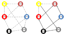
Fig. 1 (left) shows the network, indicating the possible communication links, some of which may be “closed” and “opened up” over time. The network topology is random at any time $t$, and particularly, Link 1-3 or 1-2 appears with probability $1/2$ (Fig. 1 (right)).

Figure 1: Maximal set of communication links $E_{\max}$ (left Fig.); Network topology at time $t$ (right Fig.).

For the case without delay, equation (29) is as follows:

$$\frac{dX}{d\tau}=R(\alpha,\bar{x}),$$ (58)

where

$$R(\alpha,\bar{x})=\left(\begin{array}[]{cccccc}{-1}&{\frac{1}{2}\frac{p^{2}}{p^{1}}}&{\frac{1}{2}\frac{p^{3}}{p^{1}}}&{0}&{0}&{0}\\ {0}&{-1}&{0}&{\frac{p^{4}}{p^{2}}}&{0}&{0}\\ {0}&{0}&{-1}&{0}&{\frac{p^{5}}{p^{3}}}&{0}\\ {0}&{0}&{0}&{-1}&{\frac{p^{5}}{p^{4}}}&{0}\\ {0}&{0}&{0}&{0}&{-1}&{\frac{p^{6}}{p^{5}}}\\ {\frac{p^{1}}{p^{6}}}&{0}&{0}&{0}&{0}&{-1}\end{array}\right).$$ (59)

In the case of uniformly distributed delays in the measurements, where the integer-valued delay $d_{t}^{ij}$ equals 0 or 1 with probability 1/2, $\bar{d}=1,p_{0}^{ij}=p_{1}^{ij}=1/2$, we extend the state space:

$$\bar{X}_{t}=[x_{t}^{1},\ldots,x_{t}^{n},x_{t-1}^{1},\ldots x_{t-1}^{n}]\in{\mathbb{R}}^{2n}.$$ (60)

Matrix $G$ of the corresponding averaged discrete model (39) is as follows:

$$G=\left(\begin{array}[]{cc}{\frac{1}{2}H\alpha}&{\frac{1}{2}H\alpha}\\ 0&0\end{array}\right),$$ (61)

where

$$H=\left(\begin{array}[]{cccccc}{0}&{\frac{1}{2}\frac{p^{2}}{p^{1}}}&{\frac{1}{2}\frac{p^{3}}{p^{1}}}&{0}&{0}&{0}\\ {0}&{0}&{0}&{\frac{p^{4}}{p^{2}}}&{0}&{0}\\ {0}&{0}&{0}&{0}&{\frac{p^{5}}{p^{3}}}&{0}\\ {0}&{0}&{0}&{0}&{\frac{p^{5}}{p^{4}}}&{0}\\ {0}&{0}&{0}&{0}&{0}&{\frac{p^{6}}{p^{5}}}\\ {\frac{p^{1}}{p^{6}}}&{0}&{0}&{0}&{0}&{0}\end{array}\right).$$ (68)

We set the initial queue lengths and the productivities of agents, and assume that the productivities of nodes do not change over time. In addition, we highlight that the information about the queue lengths is measured with random noise and delays.

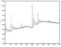
We consider two cases, the special case and the general case, as discussed in the previous subsection. We use constant step size $\alpha_{t}=\alpha=0.1$. The dynamics of the agents $x_{t}^{i}$ with local voting protocol (56) is shown in Fig. 2 and 4.

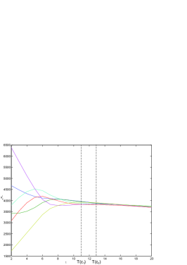
Fig. 2 shows how the system operates in the special case when there are no new incoming jobs during the system work (only the initial load). Each line, corresponding to one node, indicates how the load $x_{t}^{i}$ evolves over time. These lines also show how the system evolve to reach load-balancing or consensus.

Now we estimate the time to consensus. We calculate eigenvalues and obtain that $|Re(\lambda_{2})|=0.7737$. By formula (23) we can calculate ${T}(\varepsilon)$ for continuous system. If $\varepsilon=0.1$ then ${T}(\varepsilon)=12.8883$. If $\varepsilon=1$ then ${T}(\varepsilon)=11.4003$. The corresponding values are marked on Fig. 2.

Figure 2: Dynamics of the agents $x_{t}^{i}$ at the start and time to consensus

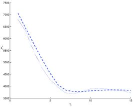
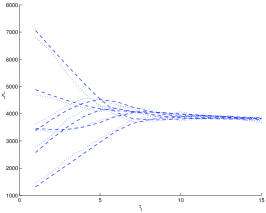
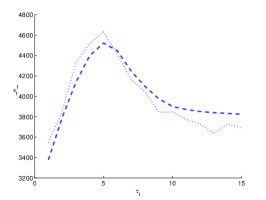
To support that we can use the averaged model to study our initial stochastic system, Fig. 3 is presented. The figure compares the dynamics of algorithm (8) and that of the averaged model described in Sec. III. Fig. 3 shows that trajectories of the stochastic discrete system (dotted lines) are close with the limiting trajectories of the average system (dashed lines).

(a) All nodes

(b) For the first node

(c) For the second node

Figure 3: Comparison of trajectories of the stochastic discrete system and its averaged model

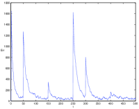
To characterize the quality of the protocol (8) in terms of convergence of trajectories to consensus $x^{\star}$, we use the average residual, defined as $Err=\sqrt{\sum_{i}\frac{(x_{t}^{i}-x^{\star})^{2}}{n}}$.

Fig. 4 shows the dynamics of the system in a more general 6-node case where new jobs can come to different agents during the system work. New jobs arrive at a random node at random times. Specifically, Fig. 4.(a) indicates how the system tries to reach consensus using the local voting protocol (8) when there are new incoming jobs. In addition, the quality of the protocol (8) is indicated by Fig. 4.(b), where the corresponding evolvement of average residuals is displayed. It shows, how the average residual changes over time: it rapidly reduces and retains at low level until new jobs received, and then it reduces again. The simulation results shows the good performance of the control protocol (8) in general case. This is explained by the properties of the stochastic approximation type algorithm with non-decreasing step, since each time instant when new jobs received might be considered as an initial time instant. In a number of similar cases the validity of applying stochastic approximation control strategies with non-decreasing to zero step sizes in nonstationary problems could be theoretically proved (see, e.g., [19, 20, 21]).

(a) Dynamics of the agents $x_{t}^{i}$

(b) Convergence to consensus

Figure 4: The 6-node general case

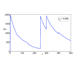
In Fig. 5 there are graphs for the average residuals with using of different parameters of step sizes $\alpha$. In first four figures we used constant step sizes. It could be seen that if we increase the step size then the time to consensus will decrease until reaching a certain level. However, if we use the decreasing step size ($\alpha_{t}=1/t$) then the convergence rate decreases with time.

Figure 5: Convergence to consensus with different step sizes.

IV-C2 The 1024-node case

To show how well the approach works to achieve load balancing and the advantage of redistribution of jobs in a larger network, we consider a network of 1024 agents. The focus here is to compare the performance of the system adopting the local voting protocol (8) to redistribute load with that without load-redistribution.

In the simulation, the time between events in the input stream is exponentially distributed with parameter $d_{in}=1/3000$, and the normalized “complexities” of jobs are also exponentially distributed with parameter $d_{p}=1$ (where, the normalized “complexity” of job is referred to as the time, required to perform the job on a single agent with productivity $p=1$). The number of incoming jobs is $10^{6}$. The choice of an agent, which receives the next job is performed randomly by the uniform distribution of 1024 agents.

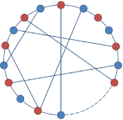
Agents are connected in a circle. In addition, there are $n$ random connections between agents on each iteration, that change over time. An example snapshot of the network is shown in Fig. 6.

Figure 6: An example of network topology.

Similarly, we also consider two cases. In the first, all jobs arrive at the initial time. In the second, the same jobs arrive at different time instants in the interval from 1 to 2000.

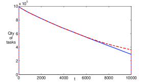
For the first case, the randomization of nodes selection at the initial time provides a uniform load (load balancing) of all nodes in the beginning, but then the strategy without redistribution begins to “lose” because the durations of jobs in the system are not known a priori, and some nodes start to “slow down”. Fig. 7 compares the number of jobs in queue with and without redistribution. Solid lines correspond to the case with redistribution of jobs by the local voting protocol, and dashed lines — to case without redistribution. The figure also shows better performance achieved by using the local voting protocol.

Figure 7: The number of jobs in the queue in case, when all jobs arrive at the initial time.

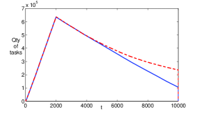
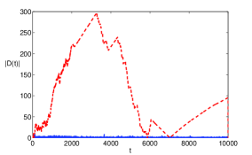
In the second case, Figs. 8 and 9 show typical results of simulations. In these figures, solid lines correspond to the case with redistribution of jobs by the local voting protocol, and dashed lines — to the case without redistribution, where symbol $|D(t)|$ stands for the maximum deviation from the average load on the network. Figs. 8 and 9 show that the performance of the adaptive multi-agent strategy with the redistribution of jobs among “connected” neighbors is significantly better than the performance of the strategy without redistribution.

Figure 8: The number of jobs in the queue in case, when all jobs arrive at different time instants.

Figure 9: Maximum deviation from the average load on the network.

V Conclusion

In this paper, the approximate consensus problem statement of multi-agent stochastic system with nonlinear dynamics, noise, delays and switched topology was introduced. In contrast to the existing stochastic approximation-based control algorithms (protocols) the local voting protocol with nonvanishing step size was proposed. Nonvanishing (e.g., constant) step size ensures better transients in the time-invariant case and provides bounded error in the case of time-varying loads and agent states. The price to pay is replacement of the mean square convergence with an approximate one.

Analytic conditions for approximate consensus in stochastic network with noise, delays and switched topology were proposed. These conditions are based on the method of averaged models. This method allows to reduce the complexity of the closed loop system analysis. In this paper, upper bounds for the mean square distance between the initial system and its approximate average model were proposed. The proposed upper bounds were used to obtain conditions for approximate consensus achievement. In contrast to our previous works, we relaxed the assumption of the weights boundedness of the protocol replacing it by the boundedness of its variances.

The theoretical results were applied to the load balancing problem in a stochastic network. Theoretical results were confirmed analytically and by simulation. The large size simulation experiments were performed for the stochastic computer network. They showed that the performance of the adaptive multi-agent strategy with the redistribution of jobs among “connected” neighbors is significantly better than the performance of the strategy without redistribution.

Appendix A Proof of Theorem 1

Proof:

The following facts will be useful, for the remainder.

Proposition 1

For $\bar{z}\in{\mathbb{R}}^{n}$ and matrix $A_{\max}$ the following inequality holds

$$\sum_{i=1}^{n}(\sum_{j\in N^{i}_{\max}}a_{\max}^{i,j}z^{j})^{2}\leq||A_{\max}||^{2}_{2}||\bar{z}||^{2}.$$ (69)

Proof:

Using the Cauchy-Schwarz inequality we obtain

$$\sum_{i=1}^{n}(\sum_{j\in N^{i}_{\max}}a_{\max}^{i,j}z^{j})^{2}\leq\sum_{i=1}^{n}(\sum_{j\in N^{i}_{\max}}{a_{\max}^{i,j}}^{2})(\sum_{j\in N^{i}_{\max}}{z^{j}}^{2})\leq$$ (70)

$$\leq(\sum_{i=1}^{n}\sum_{j=1}^{n}{a_{\max}^{i,j}}^{2})(\sum_{j=1}^{n}{z^{j}}^{2})\leq||A_{\max}||^{2}_{2}||\bar{z}||^{2}.$$

∎

For $t=1,2,\ldots$ we define an increasing sequence of $\sigma$-algebras $\tilde{\cal F}_{t}$ of probability events, generated by random elements $A_{1},\ldots,A_{t-1};$ $d_{1}^{i,j},$ $\ldots,d_{t-1}^{i,j},$ $b_{1}^{i,j},$ $\ldots,b_{t-1}^{i,j},w_{1}^{i,j},$ $\ldots,w_{t}^{i,j},$ $i,j\in N$, and ${\cal F}_{t}=\sigma\{{\cal F}_{t}^{A},A_{t};b_{t}^{i,j},d_{t}^{i,j},i,j\in N\}$.

Note that the random variables $\bar{x}_{t}$ are measurable with respect $\sigma$-algebra ${\cal F}_{t-1}$, i.e. $\mathrm{E}_{{\cal F}_{t-1}}\bar{x}_{t}=\bar{x}_{t}$.

Proposition 2

$$||\bar{s}(\bar{z})||^{2}\leq 2||{\cal L}(A_{\max})||_{2}^{2}||\bar{z}||^{2}.$$ (71)

Proof:

Using the result of Proposition 1 yields

$$||\bar{s}(\bar{z})||^{2}=\sum_{i=1}^{n}(\sum_{j=1}^{n}a_{\max}^{i,j}(z^{j}-z^{i}))^{2}\leq\sum_{i=1}^{n}(d^{i}(A_{\max})|z^{i}|+$$ (72)

$$+|\sum_{j\in N^{i}_{\max}}a_{\max}^{i,j}z^{j}|)^{2}\leq 2(\sum_{i=1}^{n}d^{i}(A_{\max})^{2}+||A_{\max}||_{2}^{2})||\bar{z}||^{2}=$$

$$2||{\cal L}(A_{\max})||_{2}^{2}||\bar{z}||^{2}.$$

∎

Proposition 3

If A2 is satisfied then $s^{i}(\bar{x})=\frac{1}{\alpha_{t}}\mathrm{E}_{{\cal F}_{t-1}}{u_{t}^{i}}$ and the following inequality holds

$$\frac{1}{\alpha_{t}^{2}}\mathrm{E}_{{\cal F}_{t-1}}{u_{t}^{i}}^{2}\leq(||\bar{x}_{t}-x_{t}^{i}\underline{1}||^{2}+\sigma_{w}^{2})\bar{b},\;i\in N.$$ (73)

Proof:

By the definition of the protocol (8)

$$\frac{1}{\alpha_{t}}u_{t}^{i}=\mathop{\sum}\limits_{j\in\bar{N}_{t}^{i}}b_{t}^{i,j}((x^{j}-x^{i})+(w_{t}^{i,j}-w_{t}^{i,i})).$$ (74)

It follows from conditions A2 that $s^{i}(\bar{x})=\frac{1}{\alpha_{t}}\mathrm{E}_{{\cal F}_{t-1}}{u_{t}^{i}}$.

By the centrality of observation noise (on condition A2a) we consecutively derive

$$\frac{1}{\alpha_{t}^{2}}\mathrm{E}_{{\cal F}_{t-1}}{u_{t}^{i}}^{2}=\mathrm{E}_{{\cal F}_{t-1}}(\mathop{\sum}\limits_{j\in\bar{N}_{t}^{i}}b_{t}^{i,j}((x_{t}^{j}-x_{t}^{i})+(w_{t}^{i,j}-w_{t}^{i,i})))^{2}=$$ (75)

$$=\mathrm{E}_{{\cal F}_{t-1}}(\mathop{\sum}\limits_{j\in\bar{N}_{t}^{i}}b_{t}^{i,j}(x_{t}^{j}-x_{t}^{i}))^{2}+\mathrm{E}_{{\cal F}_{t-1}}(\mathop{\sum}\limits_{j\in\bar{N}_{t}^{i}}b_{t}^{i,j}(w_{t}^{i,j}-w_{t}^{i,i}))^{2}\leq$$

$$\leq||\bar{x}_{t}-x_{t}^{i}\underline{1}||^{2}\mathrm{E}_{{\cal F}_{t-1}}\mathop{\sum}\limits_{j\in\bar{N}_{t}^{i}}(b_{t}^{i,j})^{2}+\mathrm{E}_{{\cal F}_{t-1}}\mathop{\sum}\limits_{j\in\bar{N}_{t}^{i}}{b_{t}^{i,j}}^{2}({w_{t}^{i,j}}^{2}+$$

$$+{w_{t}^{i,i}}^{2})\leq(||\bar{x}_{t}-x_{t}^{i}\underline{1}||^{2}+\sigma_{w}^{2})\bar{b}.$$

∎

Proposition 4

If A2 is satisfied then the following inequality holds

$$\mathrm{E}_{{\cal F}_{t-1}}|\frac{1}{\alpha_{t}}u_{t}^{i}-s^{i}(\bar{x})|^{2}\leq(n-1)\bar{b}^{2}||\bar{x}_{t}-x_{t}^{i}\underline{1}||^{2}+n\bar{b}^{2}\sigma_{w}^{2},\;i\in N.$$ (76)

Proof:

The conclusion of Proposition 4 follows from Proposition 3 since

$$\mathrm{E}_{{\cal F}_{t-1}}|\frac{1}{\alpha_{t}}u_{t}^{i}-s^{i}(\bar{x})|^{2}=(\mathrm{E}_{{\cal F}_{t-1}}\frac{1}{\alpha_{t}}u_{t}^{i})^{2}-s^{i}(\bar{x})^{2}\leq(\mathrm{E}_{{\cal F}_{t-1}}\frac{1}{\alpha_{t}}u_{t}^{i})^{2}.$$ (77)

∎

To proof the Theorem 1 we need to show that the Lipschitz and growth conditions from [46] hold. The first is a direct consequence of the Lipschitz continuous function $f^{i}(x,u)$ and the form of vector function $R(\alpha,\bar{z})$. Let $\bar{z},\bar{z}^{\prime}\in{\mathbb{R}}^{n}$. By Proposition 1 we have

$$||R(\alpha,\bar{z})-R(\alpha,\bar{z}^{\prime})||=\left(\frac{L_{1}^{2}}{\alpha^{2}}\sum_{i=1}^{n}(L_{x}|z^{i}-{z^{\prime}}^{i}|+|\alpha s^{i}(\bar{z}-\bar{z}^{\prime})|)^{2}\right)^{\frac{1}{2}}\leq$$ (78)

$$\leq L_{1}\sqrt{2}\sqrt{\frac{L_{x}}{\alpha^{2}}+2||{\cal L}(A_{\max})||_{2}^{2}}||(\bar{z}-\bar{z}^{\prime})||=\bar{L}_{1}||\bar{z}-\bar{z}^{\prime}||.$$

Similarly

$$||R(\alpha,\bar{z})-R(\alpha^{\prime},\bar{z})||=$$ (79)

$$\left(\sum_{i\in N}(\frac{1}{\alpha}f^{i}(z^{i},\alpha s^{i}(\bar{z}))-\frac{1}{\alpha^{\prime}}f^{i}(z^{i},\alpha^{\prime}s^{i}(\bar{z})))^{2}\right)^{\frac{1}{2}}=$$

$$=(\sum_{i\in N}(\frac{1}{\alpha}(f^{i}(z^{i},\alpha s^{i}(\bar{z}))-f^{i}(z^{i},\alpha^{\prime}s^{i}(\bar{z})))-$$

$$-(\frac{1}{\alpha^{\prime}}-\frac{1}{\alpha})f^{i}(z^{i},\alpha^{\prime}s^{i}(\bar{z})))^{2})^{\frac{1}{2}}\leq(2\sum_{i\in N}\frac{L_{1}^{2}(\alpha-\alpha^{\prime})^{2}}{\alpha^{2}}|s^{i}(\bar{z})|^{2}+$$

$$L_{2}(\frac{1}{\alpha^{\prime}}-\frac{1}{\alpha})^{2}(L_{c}+L_{x}|z^{i}|^{2}+{\alpha^{\prime}}^{2}|s^{i}(\bar{z})|^{2}))^{\frac{1}{2}}\leq\bar{L}_{\alpha}(1+||\bar{z}||)|\alpha-\alpha^{\prime}|.$$

Next let us prove that the growth condition. Let $\bar{z}\in{\mathbb{R}}^{n}$. Due to the limited growth rate $f^{i}(x,u)$ and Lipschitz property in $u$ (by assumption A1) we have

$${\mathrm{E}}||\frac{1}{\alpha_{t}}F(\alpha_{t},\bar{z},\bar{w}_{t})-R(\alpha,\bar{z})||^{2}=\sum_{i\in N}\mathrm{E}|\frac{1}{\alpha_{t}}f^{i}(z^{i},\alpha_{t}\tilde{s}_{t}^{i})-$$ (80)

$$-\frac{1}{\alpha}f^{i}(z^{i},\alpha s^{i}(\bar{z}))|^{2}=\sum_{i\in N}\mathrm{E}|\frac{1}{\alpha_{t}}(f^{i}(z^{i},\alpha_{t}\tilde{s}_{t}^{i})-f^{i}(z^{i},\alpha s^{i}(\bar{z})))-$$

$$-(\frac{1}{\alpha}-\frac{1}{\alpha_{t}})f^{i}(z^{i},\alpha s^{i}(\bar{z}))|^{2}\leq 2\sum_{i\in N}\mathrm{E}\frac{1}{\alpha_{t}^{2}}|f^{i}(z^{i},\alpha_{t}\tilde{s}_{t}^{i})-$$

$$-f^{i}(z^{i},\alpha s^{i}(\bar{z}))|^{2}+(\frac{1}{\alpha}-\frac{1}{\alpha_{t}})^{2}|f^{i}(z^{i},\alpha s^{i}(\bar{z}))|^{2}\leq$$

$$\leq 2\sum_{i\in N}\mathrm{E}\frac{L_{1}}{\alpha_{t}^{2}}|\alpha_{t}\tilde{s}_{t}^{i}-\alpha s^{i}(\bar{z})|^{2}+L_{2}(\frac{1}{\alpha}-\frac{1}{\alpha_{t}})^{2}(L_{c}+L_{x}|z^{i}|^{2}+$$

$$+|s^{i}(\bar{z})|^{2})\leq\gamma_{t}(nL_{c}+L_{x}||\bar{z}||^{2})+\sum_{i\in N}\mathrm{E}4L_{1}|\tilde{s}_{t}^{i}-s^{i}(\bar{z})|^{2}+$$

$$+(\frac{4L_{1}({\alpha}-{\alpha_{t}})^{2}}{\alpha_{t}^{2}}+\gamma_{t})s^{i}(\bar{z})^{2},$$

where $\gamma_{t}=2L_{2}(1/{\alpha}-1/{\alpha_{t}})^{2}$.

Denote $\beta_{t}=(4L_{1}(({\alpha}-{\alpha_{t}})^{2}-1)/\alpha_{t}^{2}+\gamma_{t}$ and by Propositions 2, 3, 4 consistently derive

$${\mathrm{E}}||\frac{1}{\alpha_{t}}F(\alpha_{t},\bar{z},\bar{w}_{t})-R(\alpha,\bar{z})||^{2}\leq\gamma_{t}(nL_{c}+L_{x}||\bar{z}||^{2})+$$ (81)

$$+\sum_{i\in N}(4\frac{L_{1}}{\alpha_{t}^{2}}(\mathrm{E}(\tilde{s}_{t}^{i})^{2}-s^{i}(\bar{z})^{2})+(\frac{4L_{1}({\alpha}-{\alpha_{t}})^{2}}{\alpha_{t}^{2}}+\gamma_{t})s^{i}(\bar{z})^{2}=$$

$$=\gamma_{t}(nL_{c}+L_{x}||\bar{z}||^{2})+4\frac{L_{1}}{\alpha_{t}^{2}}\mathrm{E}||{\tilde{s}_{t}}||^{2}+\beta_{t}||\bar{s}(\bar{z})||^{2}\leq$$

$$\leq n\gamma_{t}L_{c}+4\frac{L_{1}}{\alpha_{t}^{2}}n^{2}\bar{b}^{2}\sigma_{w}^{2}+(\gamma_{t}L_{x}+8n(n-1)\bar{b}^{2}\frac{L_{1}}{\alpha_{t}^{2}}+$$

$$+2\beta_{t}||{\cal L}(A_{\max})||_{2}^{2})||\bar{z}||^{2}=\bar{L}_{2}(1+||\bar{z}||^{2}).$$

∎

Appendix B Proof of Theorem 2

Proof:

To proof Theorem 3, the following facts will be useful.

Proposition 5

$$||U\bar{X}||^{2}\leq 2^{\tilde{d}}||\bar{X}||^{2},\;\ldots,\;||U^{\bar{d}}\bar{X}||^{2}\leq 2^{\bar{d}}||\bar{X}||^{2},\;\ldots,\;||U^{k}\bar{X}||^{2}\leq$$ (82)

$$\leq 2^{\bar{d}}||\bar{X}||^{2},$$

Proof:

By the definition of matrix $U$ it is easy to obtain the first inequality, and the rest we get by induction on $k$ and by the following equality

$$\forall k>\bar{d}\;\;U^{k}=U^{\bar{d}}=\left(\begin{array}[]{ccccc}{I}&{0}&{0}&{\ldots}&{0}\\ {I}&{0}&{0}&{\ldots}&{0}\\ {\vdots}&{\vdots}&{\vdots}&{\vdots}&{\vdots}\\ {I}&{0}&{0}&{\ldots}&{0}\end{array}\right).$$ (83)

∎

Denote

$$v_{t}=F(\alpha_{t},\bar{X}_{t},\bar{w}_{t})-G(\alpha_{t},\bar{X}_{t}).$$ (84)

Proposition 6

By assumptions A2 the following inequality holds

$$\mathrm{E}\max_{1\leq t\leq T}||\sum_{i=1}^{t}v_{t}||^{2}\leq 4n\sum_{t=1}^{T}\mathrm{E}||v_{t}||^{2}.$$ (85)

Proof:

Under the conditions A2 random elements $v_{t}$ are martingale differences, i.e., they are centered with respect to the conditional averaging of the background: $\mathrm{E}_{{\cal F}_{t-1}}v_{t}=0$. So, Lemma 1 from section 3 of [47] is applicable. The dimension of vectors $v_{t}$ is $n\bar{d}$, but since only the first $n$ components of vectors $v_{t}$ are nonzero, then it is possible to use in the estimation the value of $n$ instead of $n\bar{d}$. ∎

Proposition 7

Let the sequence of numbers $\mu_{t}\geq 0$, $t=0,1,\ldots,T$ satisfies the inequalities

$$\mu_{t+1}\leq\bar{\alpha}c_{1}\tau_{t}+c_{2}2^{\bar{d}}\tau_{t}\sum_{k=1}^{t}\gamma_{k}\mu_{k},\;c_{1},c_{2}\geq 0,\;$$ (86)

then

$$\mu_{t}\leq c_{1}\tau_{t}e^{c_{2}\tau_{t}^{2}}\bar{\alpha}.$$ (87)

Proof:

Statement of Proposition follows directly from the corresponding result in [48] ∎

Proposition 8

By assumptions A1, A2 yields

$$\mathrm{E}||\bar{X}_{t}||^{2}\leq(\frac{2nL_{2}+\bar{\alpha}^{2}\tilde{c}}{c_{3}}+||\bar{X}_{0}||^{2})e^{t\ln(c_{3}+1)}.$$ (88)

Proof:

We write equation (36) as

$$\bar{X}_{t+1}=U\bar{X}_{t}+G(\alpha_{t},\bar{X}_{t})+v_{t}.$$ (89)

For the squared norm of $\bar{X}_{t+1}$ we have

$$||\bar{X}_{t+1}||^{2}=||U\bar{X}_{t}+G(\alpha_{t},\bar{X}_{t})||^{2}+2(U\bar{X}_{t}+G(\alpha_{t},\bar{X}_{t}))^{\rm T}v_{t}+||v_{t}||^{2}.$$ (90)

Taking the conditional expectation of both parts of (90) on $\sigma$-algebra ${\cal F}_{t-1}$ (i.e. for fixed $\bar{X}_{t}$) by the centrality of $v_{t}$ we obtain

$$\mathrm{E}_{{\cal F}_{t-1}}{||\bar{X}_{t+1}||^{2}}=||U\bar{X}_{t}+G(\alpha_{t},\bar{X}_{t})||^{2}+\mathrm{E}_{{\cal F}_{t-1}}||v_{t}||^{2}\leq$$

$$\leq 2||U\bar{X}_{t}||^{2}+2||G(\alpha_{t},\bar{X}_{t})||^{2}+\mathrm{E}_{{\cal F}_{t-1}}||v_{t}||^{2}.$$ (91)

By the form of $v_{t}$ and Lipschitz in $u$ of functions $f^{i}(u)$ (by A1) for $||v_{t}||^{2}$ we have

$$||v_{t}||^{2}=\sum_{i\in N}|f^{i}(x_{t}^{i},\alpha_{t}\mathop{\sum}\limits_{j\in\bar{N}_{t}^{i}}b_{t}^{i,j}(x_{t-d_{t}^{i,j}}^{j}-x_{t}^{i}+w_{t}^{i,j}-w_{t}^{i,i}))-$$ (92)

$$-f^{i}(x_{t}^{i},{\alpha_{t}}s^{i}_{t}(\bar{X}_{t}))|^{2}\leq L_{1}^{2}||\bar{u}_{t}-\alpha_{t}^{2}\bar{s}_{t}||^{2}.$$

Under the conditions A2, random variables $\mathrm{E}_{{\cal F}_{t-1}}u^{i}_{t}$, $i\in N$ satisfy the conditions of Proposition 3

$$\mathrm{E}_{{\cal F}_{t-1}}||v_{t}||^{2}=\alpha_{t}^{2}L_{1}^{2}(2n\bar{b}||\bar{X}_{t}||^{2}+n^{2}\bar{b}\sigma_{w}^{2}).$$ (93)

Consistently evaluating all three summands on the right hand side of (91) and taking into account the results of Propositions 5, 2 and 3, we deduce

$$\mathrm{E}_{{\cal F}_{t}}{||\bar{X}_{t+1}||^{2}}\leq 2^{\tilde{d}}||\bar{X}_{t}||^{2}+2^{1+\tilde{d}/2}||\bar{X}_{t}||L_{1}(L_{x}||\bar{X}_{t}||+{\alpha_{t}}||\bar{s}||)+$$ (94)

$$+L_{2}(nL_{c}+L_{x}||\bar{X}_{t}||^{2}+{\alpha_{t}^{2}}||\bar{s}||^{2})+\alpha_{t}^{2}L_{1}^{2}(2n\bar{b}||\bar{X}_{t}||^{2}+$$

$$+2n\bar{b}\sigma_{w}^{2})\leq(2^{\tilde{d}}+2^{1+\tilde{d}/2}L_{1}L_{x}+L_{2}L_{x}+\alpha_{t}2^{1+\tilde{d}/2}L_{1}||{\cal L}(A_{\max})||_{2}+$$

$$+{\alpha_{t}^{2}}(L_{2}||{\cal L}(A_{\max})||_{2}^{2}+2nL_{1}^{2}\bar{b}))||\bar{X}_{t}||^{2}+nL_{2}L_{c}+$$

$$+2{\alpha_{t}^{2}}nL_{1}^{2}\bar{b}\sigma_{w}^{2}\leq\bar{c}+\bar{c}_{3}||\bar{X}_{t}||^{2},$$

where $\bar{c}=nL_{2}L_{c}+{\alpha_{t}^{2}}\tilde{c},\;\bar{c}_{3}=c_{3}+1.$

By taking unconditional expectation of both parts of this inequality and consistently iterating on $t$, we obtain Proposition 8

$$\mathrm{E}||\bar{X}_{t}||^{2}\leq\bar{c}+\bar{c}_{3}\mathrm{E}||\bar{X}_{t-1}||^{2}\leq\bar{c}+\bar{c}\bar{c}_{3}+\bar{c}_{3}^{2}\mathrm{E}||\bar{X}_{t-2}||^{2}\leq$$ (95)

$$\leq\bar{c}(1+\bar{c}_{3}+\bar{c}_{3}^{2}+\ldots+\bar{c}_{3}^{t-1})+\bar{c}_{3}^{t}||\bar{X}_{0}||^{2}\leq\bar{c}\frac{\bar{c}_{3}^{t}-1}{c_{3}}+\bar{c}_{3}^{t}||\bar{X}_{0}||^{2}\leq$$

$$\leq\left(\frac{\bar{c}}{c_{3}}+||\bar{X}_{0}||^{2}\right)\bar{c}_{3}^{t}\leq(\bar{c}_{4}+||\bar{X}_{0}||^{2})e^{t\ln\bar{c}_{3}},$$

where $\bar{c}_{4}={\bar{c}}/{c_{3}}$. ∎

Denote $x^{\star}$ as the consensus value of the continuous model. From the first group of conditions of Theorem 2 the conditions of Theorem 1 hold, i.e. the result of the theorem is true. From other conditions of Theorem 2 and the result of Theorem 1 we obtain

$$\mathrm{E}||\bar{x}_{t}-x^{\star}\underline{1}||^{2}\leq 2\mathrm{E}||\bar{x}_{t}-\bar{x}(\tau)||^{2}+2||\bar{x}(\tau)-x^{\star}\underline{1}||^{2}\leq\frac{\varepsilon}{2}+\frac{\varepsilon}{2}\leq\varepsilon.$$ (96)

∎

Appendix C Proof of Corollary 1

Proof:

In the conditions of Corollary 1 $R(\alpha,\bar{x})$ is a linear function. Therefore the dynamical system (29) takes the form:

$$\dot{\bar{x}}=-{\cal L}(A_{\max})\bar{x},$$ (97)

where ${\cal L}(A_{\max})$ is the Laplacian of $A_{\max}$. All amounts in rows of elements of the matrix ${\cal L}(A_{\max})$ are equal to zero and, moreover, all the diagonal elements are positive and equal to the absolute value of the sum of all the other elements in the row. The vector of 1’s $\underline{1}$ is the right eigenvector corresponding to zero eigenvalue. The resulting continuous system is partially stable with respect to $h=\underline{1}^{T}\bar{x}$.

By condition A3 it was obtained that in this continuous system the asymptotic consensus is achieved, and in Lemma 5 the $\varepsilon$-consensus is achieved, and the time to consensus is given by (23).

∎

Appendix D Proof of Theorem 3

Proof:

By condition A2 averaging with respect to $\sigma$-algebras ${\cal F}_{t}^{d}$ and ${\cal F}_{t}$ yields $\mathrm{E}_{{\cal F}_{t}}v_{t}=0$. By iterating equation (36) for $t,t-1,\ldots t-d+1$ we obtain

$$\bar{X}_{t+1}=U\bar{X}_{t}+G(\alpha_{t},\bar{X}_{t})+v_{t}=$$

$$=U^{2}\bar{X}_{t-1}+UG(\alpha_{t-1},\bar{X}_{t-1})+G(\alpha_{t},\bar{X}_{t})+Uv_{t-1}+v_{t}=$$ (98)

$$=\cdots=U^{t+1}\bar{X}_{0}+\sum_{k=0}^{t}U^{t-k}G(\alpha_{k},\bar{X}_{k})+\sum_{k=0}^{t}U^{t-k}v_{k}.$$

Similarly we obtain

$$\bar{Z}_{t+1}=U^{t+1}\bar{X}_{0}+\sum_{k=0}^{t}U^{t-k}G(\alpha_{k},\bar{Z}_{k}).$$ (99)

Let us estimate $||\bar{X}_{t}-\bar{Z}_{t}||^{2},\;t=1,\ldots,T$. By subtracting (99) from (98) and squaring the result we obtain

$$||\bar{X}_{t}-\bar{Z}_{t}||^{2}=||\sum_{k=1}^{t}U^{t-k}v_{k}+\sum_{k=1}^{t}U^{t-k}(G(\alpha_{k},\bar{X}_{k})-G(\alpha_{k},\bar{Z}_{k}))||^{2}\leq$$

$$\leq 2||\sum_{k=1}^{t}U^{t-k}v_{k}||^{2}+2||\sum_{k=1}^{t}U^{t-k}(G(\alpha_{k},\bar{X}_{k})-G(\alpha_{k},\bar{Z}_{k}))||^{2}\leq$$

$$\leq 2||\sum_{k=1}^{t}U^{t-k}v_{k}||^{2}+2\frac{\tau_{t}}{2^{\bar{d}}}\sum_{k=1}^{t}\frac{1}{\alpha_{t}}||U^{t-k}(G(\alpha_{k},\bar{X}_{k})-G(\alpha_{k},\bar{Z}_{k}))||^{2}.$$ (100)

For the summands in the second sum of (100) using Propositions 2, 5 and Lipschitz condition $f^{i}(\cdot,\cdot)$ (assumption A1) we obtain

$$||U^{t-k}(G(\alpha_{k},\bar{X}_{k})-G(\alpha_{k},\bar{Z}_{k}))||^{2}\leq 2^{\bar{d}}L_{1}^{2}\sum_{i=1}^{n}(L_{x}|x^{i}_{k}-z^{i}_{k}|+$$ (101)

$$+\alpha_{k}|s(x^{i}_{k})-s(z^{i}_{k})|)^{2}\leq 2^{1+\bar{d}}L_{1}^{2}\sum_{i=1}^{n}L_{x}|x^{i}_{k}-z^{i}_{k}|^{2}+\alpha_{k}^{2}s(x^{i}_{k}-z^{i}_{k})^{2}\leq$$

$$\leq 2^{1+\bar{d}}L_{1}^{2}(L_{x}+2\alpha_{k}^{2}||{\cal L}(A_{\max})||_{2}^{2})||\bar{X}_{k}-\bar{Z}_{k}||^{2}$$

We take expectation of both parts of (100) and denote $\mu_{T}=\mathop{\max}\limits_{0\leq{t}\leq T}\mathrm{E}||\bar{X}_{t}-\bar{Z}_{t}||^{2}$. By applying Proposition 6 to the first summand and obtained above estimate of the second summand we obtain

$$\mu_{T}\leq 2^{3+\bar{d}}n\sum_{k=1}^{T}\mathrm{E}||v_{k}||^{2}+2\tau_{T}L_{1}^{2}\sum_{k=1}^{t}(\frac{L_{x}}{\underline{\alpha}}+2\alpha_{k}||{\cal L}(A_{\max})||_{2}^{2})\mu_{k}.$$ (102)

To estimate $\mathrm{E}||v_{k}||^{2}$ by using previously obtained relation (93) and the result of Proposition 8 we deduce

$$\mathrm{E}||v_{k}||^{2}\leq\alpha_{k}^{2}(\tilde{c}+\hat{c}(\bar{c}_{4}+||\bar{X}_{0}||^{2})e^{k\ln(c_{3}+1)})$$ (103)

and hence

$$2^{3+\bar{d}}n\sum_{k=1}^{T}\mathrm{E}||v_{k}||^{2}\leq\bar{\alpha}8n\tau_{T}(\tilde{c}+\hat{c}(\bar{c}_{4}+||\bar{X}_{0}||^{2})e^{T\ln(c_{3}+1)}).$$ (104)

By the following relation $2^{\bar{d}}\sum_{k=1}^{t}\alpha_{k}^{2}\leq\bar{\alpha}2^{\bar{d}}\sum_{k=1}^{t}\alpha_{k}=\bar{\alpha}\tau_{t},$ considering estimates (104) from (102), we have

$$\mathrm{E}\mu_{T}\leq\bar{\alpha}c_{1}\tau_{T}+c_{2}\tau_{T}2^{\bar{d}}\sum_{k=1}^{T}\alpha_{k}\mathrm{E}\mu_{k}.$$ (105)

From last inequality (105) by applying Proposition 7 we get the conclusion of Theorem 3. ∎

Appendix E Proof of Theorem 4

Proof:

Denote $x^{\star}$ as consensus value of discrete system (39). From the first group of conditions of Theorem 4 the conditions of Theorem 3 hold. From other conditions of Theorem 4 and the result of Theorem 3 we obtain

$$\mathrm{E}||\bar{X}_{t}-x^{\star}\underline{1}||^{2}\leq 2\mathrm{E}||\bar{X}_{t}-\bar{Z}_{t}||^{2}+2||\bar{Z}_{t}-x^{\star}\underline{1}||^{2}\leq\frac{\varepsilon}{2}+\frac{\varepsilon}{2}\leq\varepsilon.$$ (106)

∎

Appendix F Proof of Theorem 5

Proof:

The result of Theorem 5 is derived from Theorem 4.

All amounts in rows of elements of the matrix $\bar{\cal L}=(I-U)-{\cal L}(\alpha A_{\max})$ are equal to zero and, moreover, all the diagonal elements are positive and equal to the absolute value of the sum of all the other elements in the row, which are negative. Hence the matrix $\bar{\cal L}$ is the Laplacian of a graph and a vector of 1’s $\underline{1}$ is the right eigenvector corresponding to zero eigenvalue.

By condition A3, the graph corresponding to the Laplacian $\bar{\cal L}$ has a spanning tree. By condition A3 graph of the first $n$ nodes has a spanning tree. And units on $(n+1)$-th diagonal consistently connect $\bar{n}$-th node with $(\bar{n}-\bar{d})$-th node, $(\bar{n}-1)$-th node with $(\bar{n}-\bar{d}-1)$-th and so on. Hence the asymptotic consensus is achieved in such a discrete system since the condition $\alpha<\frac{1}{d_{\max}}$ holds by the assumptions of Theorem 5.

To satisfy the conditions of Theorem 4 it remains to show that the constants $\bar{C}_{1}$ and $\bar{C}_{2}$ are the same as the corresponding constants from Theorem 3. It follows from the fact that in this case $L_{1}=L_{2}=1$, $L_{x}=L_{c}=0$. ∎

Appendix G Proof of Lemma 6

Proof:

We take $x_{t}^{i}=q_{t}^{i}/p_{t}^{i}$ as the state of agent $i$.

We give the proof by contradiction. Assume that for some optimal strategy not all $x_{t}^{i}$ are equal to each other, i.e. there is a agent with the number $k\in N$ and the subset of agents $\tilde{N}_{t}$ such that $x_{t}^{k}>x_{t}^{j},\;\forall j\;\in\tilde{N}_{t}$.

Denoted by $l=|\tilde{N}_{t}|$ the number of agents in $\tilde{N}_{t}$. The states of other $n-l$ agents equal $x_{t}^{k}$.

Let the difference between the state of $k$-th agent and the biggest of the set $\tilde{N}_{t}$ equals to $\epsilon_{t}$, i.e.

$$\epsilon_{t}=x_{t}^{k}-\max_{j\;\in\tilde{N}_{t}}x_{t}^{j}.$$ (107)

Let’s consider the new strategy of job redistribution. Reduce the load of all $n-l$ agents which have the maximum load on $\frac{\epsilon}{2(n-l)}$ (i.e. on $\frac{\epsilon}{2}$ at all) and add this $\frac{\epsilon}{2}$ jobs to any of the $l$ agents of $\tilde{N}_{t}$. For new strategy we found that the time of job redistribution in the system will be less than the initial on the $\frac{\epsilon}{2(n-l)}$, i.e. less than the minimum by the assumption. A contradiction.

∎

Appendix H Proof of Theorem 6

Proof:

You should verify if the conditions A1, A2 for the considered control protocol and functions $f^{i}(\cdot,\cdot)$ are satisfied. If they are satisfied, then all the conditions of Theorem 4 are satisfied and the result is valid for this case.

The condition A1 holds since the function $f^{i}(x,u)=-1+u$ is linear in $u$. The condition A2 holds because of the formation rules for the weighting coefficients in the control protocol and stabilization conditions for $p_{t}^{i}$.

∎

References

• [1] R. Olfati-Saber, J. Fax, and R. Murray, “Consensus and cooperation in networked multi-agent systems,” Proceedings of the IEEE, vol. 95, no. 1, pp. 215–233, 2007.
• [2] W. Ren, R. Beard, and E. Atkins, “Information consensus in multivehicle cooperative control,” Control Systems, IEEE, vol. 27, no. 2, pp. 71–82, 2007.
• [3] C. Wu, Synchronization in complex networks of nonlinear dynamical systems.   World Scientific Publishing Company Incorporated, 2007.
• [4] W. Ren and R. Beard, Distributed consensus in multi-vehicle cooperative control: theory and applications.   Springer, 2007.
• [5] F. Bullo, J. Cortés, and S. Martinez, Distributed control of robotic networks: a mathematical approach to motion coordination algorithms.   Princeton University Press, 2009.
• [6] P. Antsaklis and J. Baillieul, “Guest editorial special issue on networked control systems,” Automatic Control, IEEE Transactions on, vol. 49, no. 9, pp. 1421–1423, 2004.
• [7] C. Abdallah and H. Tanner, “Complex networked control systems: introduction to the special section,” Control Systems, IEEE, vol. 27, no. 4, pp. 30–32, 2007.
• [8] P. Antsaklis and J. Baillieul, “Special issue on technology of networked control systems,” Proceedings of the IEEE, vol. 95, no. 1, pp. 5–8, 2007.
• [9] D. Armbruster, A. Mikhailov, K. Kaneko et al., Networks of Interacting Machines: Production Organization in Complex Industrial Systems and Biological Cells.   World Scientific. Singapore, 2005.
• [10] O. Granichin, P. Skobelev, A. Lada, I. Mayorov, and A. Tsarev, “Comparing adaptive and non-adaptive models of cargo transportation in multi-agent system for real time truck scheduling,” in Proc. 4th International Conference on Computational Intelligence. Evolutionary Computation Theory and Applications (ECTA 2012), Barcelona, Spain, 2012, pp. 282–285.
• [11] M. Huang and J. Manton, “Coordination and consensus of networked agents with noisy measurements: stochastic algorithms and asymptotic behavior,” SIAM Journal on Control and Optimization, vol. 48, no. 1, pp. 134–161, 2009.
• [12] R. Rajagopal and M. Wainwright, “Network-based consensus averaging with general noisy channels,” Signal Processing, IEEE Transactions on, vol. 59, no. 1, pp. 373–385, 2011.
• [13] L. Wang, Z. Liu, and L. Guo, “Comparing adaptive and non-adaptive models of cargo transportation in multi-agent system for real time truck scheduling,” in Proc. of the 26th Chinese Control Conference, Zhangjiajie, Hunan, China, 2007, pp. 737–741.
• [14] R. Olfati-Saber and R. Murray, “Consensus problems in networks of agents with switching topology and time-delays,” Automatic Control, IEEE Transactions on, vol. 49, no. 9, pp. 1520–1533, 2004.
• [15] W. Ren and R. Beard, “Consensus seeking in multiagent systems under dynamically changing interaction topologies,” Automatic Control, IEEE Transactions on, vol. 50, no. 5, pp. 655–661, 2005.
• [16] J. Tsitsiklis, D. Bertsekas, and M. Athans, “Distributed asynchronous deterministic and stochastic gradient optimization algorithms,” Automatic Control, IEEE Transactions on, vol. 31, no. 9, pp. 803–812, 1986.
• [17] T. Li and J. Zhang, “Mean square average-consensus under measurement noises and fixed topologies: Necessary and sufficient conditions,” Automatica, vol. 45, no. 8, pp. 1929–1936, 2009.
• [18] M. Huang, “Stochastic approximation for consensus: a new approach via ergodic backward products,” IEEE Transactions on Automatic Control, vol. 57, no. 12, pp. 2994–3008, 2012.
• [19] A. Vakhitov, V. Vlasov, and O. Granichin, “Adaptive control of siso plant with time-varying coefficients based on random test perturbation,” in Proc. American Control Conference (ACC), 2010.   Baltimore, Maryland, USA: IEEE, 2010, pp. 4004–4009.
• [20] A. Vakhitov, O. Granichin, and L. Gurevich, “Algorithm for stochastic approximation with trial input perturbation in the nonstationary problem of optimization,” Automation and Remote Control, vol. 70, no. 11, pp. 1827–1835, 2009.
• [21] O. Granichin, L. Gurevich, and A. Vakhitov, “Discrete-time minimum tracking based on stochastic approximation algorithm with randomized differences,” in Proc. 48th IEEE Conference on Decision and Control, 2009 held jointly with the 2009 28th Chinese Control Conference. CDC/CCC 2009.   Shanghai, China: IEEE, 2009, pp. 5763–5767.
• [22] V. Borkar, “Stochastic approximation: a dynamical systems viewpoint,” 2008.
• [23] T. Friedrich, T. Sauerwald, and D. Vilenchik, “Smoothed analysis of balancing networks,” Random Structures & Algorithms, vol. 39, no. 1, pp. 115–138, 2010.
• [24] H. Li, “Load balancing algorithm for heterogeneous p2p systems based on mobile agent,” in Electric Information and Control Engineering (ICEICE), 2011 International Conference on, Wuhan, China, 2011, pp. 1446–1449.
• [25] M. Kechadi, I. Savvas et al., “Dynamic task scheduling for irregular network topologies,” Parallel Computing, vol. 31, no. 7, pp. 757–776, 2005.
• [26] G. Cybenko, “Dynamic load balancing for distributed memory multiprocessors,” Journal of parallel and distributed computing, vol. 7, no. 2, pp. 279–301, 1989.
• [27] Y. Li and Z. Lan, “A survey of load balancing in grid computing,” Computational and Information science, pp. 280–285, 2005.
• [28] K. Gilly, C. Juiz, and R. Puigjaner, “An up-to-date survey in web load balancing,” World Wide Web, vol. 14, no. 2, pp. 105–131, 2011.
• [29] K. Sim and W. Sun, “Ant colony optimization for routing and load-balancing: survey and new directions,” Systems, Man and Cybernetics, Part A: Systems and Humans, IEEE Transactions on, vol. 33, no. 5, pp. 560–572, 2003.
• [30] O. Granichin, “Stochastic optimization and system programming,” Stochastic Optimization in Informatics, vol. 6, pp. 3–44, 2010.
• [31] A. Vakhitov, O. Granichin, and M. Panshenskov, “Methods of data transfer speed estimation in the data grid based on linear regression,” Neurocomputers: design, application, no. 11, pp. 45–52, 2009.
• [32] N. Amelina, A. Fradkov, and K. Amelin, “Approximate consensus in multi-agent stochastic systems with switched topology and noise,” in Proc. IEEE 2012 Multiconference on Systems and Control (MSC 2012), Dubrovnik, Croatia, 2012, pp. 445–450.
• [33] N. Amelina and A. Fradkov, “Approximate consensus in the dynamic stochastic network with incomplete information and measurement delays,” Automation and Remote Control, vol. 73, no. 11, pp. 1765 –1783, 2012.
• [34] K. Amelin, N. Amelina, O. Granichin, and O. Granichina, “Multi-agent stochastic systems with switched topology and noise,” in Proc. 2012 13th ACIS International Conference on Software Engineering, Artificial Intelligence, Networking and Parallel & Distributed Computing (SNPD), Kyoto, Japan, 2012, pp. 438–443.
• [35] N. Amelina, “Scheduling networks with variable topology in the presence of noise and delays in measurements,” Vestnik St. Petersburg University: Mathematics, vol. 45, no. 2, pp. 56–60, 2012.
• [36] N. Amelina and A. Fradkov, “Consensus problem in stochastic network systems with switched topology, noise and delay,” in Proc. The Twelfth International Conference on Networks (ICN 2013).   Seville, Spain: IARIA, 2013, pp. 118–124.
• [37] D. Derevitskii and A. Fradkov, “Two models for analysis the dynamics of adaptation algorithms,” Automation and Remote Control, no. 1, pp. 59–67, 1974.
• [38] L. Ljung, “Analysis of recursive stochastic algorithms,” Automatic Control, IEEE Transactions on, vol. 22, no. 4, pp. 551–575, 1977.
• [39] H. Kushner, “Convergence of recursive adaptive and identification procedures via weak convergence theory,” Automatic Control, IEEE Transactions on, vol. 22, no. 6, pp. 921–930, 1977.
• [40] R. Agaev and P. Chebotarev, “The matrix of maximal outgoing forests of a digraph and its applications,” Automation and Remote Control, vol. 61, no. 9, pp. 1424 –1450, 2000.
• [41] S. Gershgorin, “On bounding the eigenvalues of a matrix,” Izv. Akad. Nauk. SSSR Otd Mat. Estest 1, no. 6, pp. 749–754 749–754, 1931.
• [42] F. Lewis, “Book chapter 1 – first-order consensus,” EE 5329 Distributed Decision and Control COURSE NOTES.
• [43] L. Gerencsér, “A representation theorem for the error of recursive estimators,” SIAM journal on control and optimization, vol. 44, no. 6, pp. 2123–2188, 2006.
• [44] K. Amelin, N. Amelina, O. Granichin, and A. Koryavko, “Local voting algorithm for consensus problem in decentralized network of intelligent agents,” Neurocomputers: design, application, no. 11, pp. 39–47, 2012.
• [45] K. Amelin, “Randomization in control for a small uav fly optimization under unknown arbitrary wind disturbances,” Cybernetics and Physics, vol. 1, no. 2, pp. 79–88, 2012.
• [46] A. Fradkov, “Continuous-time averaged models of discrete-time stochastic systems: Survey and open problems,” in Proc. 2011 50th IEEE Conference on Decision and Control and European Control Conference (CDC-ECC).   Orlando, Florida, USA: IEEE, 2011, pp. 2076–2081.
• [47] I. Gihman and A. Skorohkod, Stochastic Differential Equations.   Kiev: Nauk. dumka, 1968.
• [48] S. Bernstein, “Stochastic difference equations and stochastic differential equations,” Sobr. soch. in 4-th Vol., vol. 4, pp. 484–542, 1964.