Strong coupling and quark masses from lattice QCD

Abstract

I review lattice QCD calculations of the strong coupling and quark masses.

Received (Day Month Year)Revised (Day Month Year)

PACS Nos.: 12.38.Gc; 12.15.Ff.

1 Introduction

I review recent lattice QCD calculations of the strong coupling and quark masses. It is very timely to do this because the errors on these quantities from the PDG [1] have been reduced this year.

The basic theory behind the calculation of the properties of bound states of QCD, using lattice QCD, is the creation and destruction of particles in the path integral formalism.

$$c_{ij}(t)=\frac{1}{Z}\int du\int d\psi\overline{d\psi}O(t)_{i}O(0)_{j}^{\dagger}e^{-S_{F}-S_{G}}$$ (1)

where the $S_{F}$ is the action for the quarks and $S_{G}$ is the action for the gauge fields. The path integral is regulated by the introduction of a space-time lattice and is computed in Euclidean space using Monte Carlo techniques on the computer. The final stage of the calculation is a set of physical quantities, such as a meson mass, for a specific lattice coupling, volume and input quark masses. The physical quantities are extrapolated to the continuum limit, infinite volume and physical quark masses.

Table 1: Parameters of two recent lattice QCD calculations.

Action	$n_{f}$	lattice spacing		$m_{\pi}$		$m_{\pi}L$
		No.	Range fm	No.	Range MeV
HISQ [2]	2+1+1	3	0.15 - 0.06	$>3$	128 - 312	3.22 - 5.36
2 HEX Clover [3]	2+1	5	0.12 - 0.065	$>5$	120 - 670	3.0 - 6.36

The solution of Eq. 1 solves QCD, at the input parameters, however the key issue is how physical the parameters are and so for example whether a controlled continuum limit can be taken. The computational cost of the lattice QCD calculation depends particularly on the masses of the light quarks and on the type of lattice approximation to the Dirac operator used. In table 1 I report the parameters of two recent lattice QCD calculations (see  [4] for a more complete review).

It is important to compute experimental numbers as a cross-check on the lattice QCD calculation. BMW-c [5] have accurately computed 10 ground state hadron masses from a 2+1 unquenched lattice QCD calculation. The continuum limit was taken and the lightest pion mass was 190 MeV. The HPQCD collaboration [6] have published a summary plot of the masses of 22 mesons, some of which are predictions, which include the bottom or charm quarks.

I exclusively focus on the results of recent lattice QCD calculations. Motivated by the FLAG [7] group’s review system, I plot the lattice results for quark masses in green if the systematics are under reasonable control, but use red if more work is required, because for example only one lattice spacing is used. For the $\alpha_{s}$ summary I use green or red circles for the quality of the continuum and chiral limit.

2 Quark masses from lattice QCD

Quark masses are inputted to the lattice QCD calculation and a subset of the hadron spectrum is computed in lattice units. The quark masses are chosen to reproduce the masses of a few hadrons. The lattice spacing is also determined from a physical quantity. After the bare quark masses have been determined they need to be converted into a continuum scheme.

$$m_{q}^{\overline{MS}}(\mu)=Z^{\overline{MS}}_{m}(\mu)m_{q}^{bare}$$ (2)

The $Z^{\overline{MS}}_{m}(\mu)$ factors in Eq. 2 can be computed using lattice perturbation theory, or a variety of numerical techniques [8, 9, 10], which compute the lattice contribution to $Z^{\overline{MS}}_{m}(\mu)$ to all orders. The quark mass is usually required at a standard scale, such as 2 or 3 GeV, or the mass of the quark itself. The numerical technique to compute $Z^{\overline{MS}}_{m}(\mu)$ usually only works for a window of momentum, so some evolution of the quark masses with scale may be required.

The ratios of quark masses, such as $m_{c}/m_{s}$, $m_{b}/m_{c}$, $2m_{s}/(m_{d}+m_{u})$ are independent of renormalisation, hence are now commonly computed.

3 The QCD coupling

As in the continuum the basic idea of determining the QCD coupling is to compute some quantity $\sigma$ in the lattice QCD calculation, which has a perturbative expansion.

$$\sigma=a_{0}+\alpha_{s}a_{1}+\alpha_{s}^{2}a_{2}+\alpha_{s}^{3}a_{3}+....$$ (3)

The coefficients $a_{i}$ are computed in perturbation theory but also typically contain non-perturbative contributions. Lattice perturbation theory can be used, or it is usually easier to take the continuum limit of a quantity and then use continuum perturbation theory, because higher order calculations are easier in the continuum.

The contribution of the charm and bottom quarks are perturbatively added to $\alpha_{s}$ extracted from a lattice QCD calculation with 2+1 flavors of sea quarks. The coupling is then evolved typically using perturbation theory to the mass of the Z boson. The inclusion of a quark’s contribution using perturbation theory is done at the scale of quark mass. There are concerns that perturbation is not reliable at the scale of the charm mass (1.2 GeV), although this matching is not a significant contribution to the error from [11]. The matching of the results for $\alpha_{s}$ from calculations with $n_{f}=2$ to $n_{f}=5$ is more problematic (see Ref. [12] for a review plot which includes $n_{f}=2$ results), because it must be done at the scale of 100 MeV.

The HPQCD collaboration [11] have computed $\alpha_{s}$ by measuring 22 different combinations of small Wilson loops in the numerical lattice QCD calculation and comparing them to expressions in lattice perturbation theory. The perturbative calculation included terms of $\alpha_{s}^{3}$ and has been checked by Trottier and Wong using a numerical technique [13]. There are small non-perturbative contributions to Wilson loops from condensates, such as the non-perturbative gluon condensate, which increase with the size of the loop. The lattice spacing was obtained from the $\Upsilon$ spectrum and $f_{\pi}$. The calculation used data at 6 different lattice spacings,

The HPQCD collaboration [14, 15] have used the moments of correlators to compute the masses of the charm and bottom quarks, as well as the strong coupling. In the lattice QCD calculation the time moments of the correlator in Eq. 1 are measured.

$$G_{n}\equiv\sum_{t}(t/a)^{n}c_{11}(t)$$ (4)

The moments of the correlators are analyzed using continuum perturbation theory after the continuum limit is taken. The $G_{4}$ moment is insensitive to the heavy quark mass, so it is used to estimate $\alpha_{s}$. The first paper [14] on using moments in an unquenched calculation was a collaboration between the HPQCD collaboration and Chetyrkin, Kühn, Steinhauser,Sturm. There was an updated result [15].

The JLQCD collaboration have extracted $\alpha_{s}$ from the light vacuum polarization [16].

$$\langle J^{a}_{\mu}J^{b}_{\nu}\rangle(Q)=\delta^{ab}\left[(\delta_{\mu\nu}Q^{2}-Q_{\mu}Q_{\nu})\Pi_{J}^{(1)}(Q)-Q_{\mu}Q_{\nu}\Pi_{J}^{(0)}(Q)\right],$$ (5)

and $Q_{\mu}$ is space-like and $J_{\mu}=V_{\mu}$ vector and $J_{\mu}=A_{\mu}$ for the axial current. The correlators for the sum $\Pi_{V}(Q)+\Pi_{A}(Q)$ were fitted to an OPE based formulae using continuum perturbation theory known up the 4 loops for some cases. The calculation also used condensates, either measured from other lattice calculations or taken from phenomenology. The continuum limit was not taken.

The strong coupling has recently been computed by Bazavov et al. [17] from the measured static QCD potential on the lattice. The static energy has recently been computed to $N^{3}LL$ in perturbation theory [18, 19]. The basis of the lattice QCD calculation was gauge configurations generated by the HOT collaboration generated as the T=0 part of thermodynamic project. Eight lattice spacings in the range: 0.805 GeV $<$ $a^{-1}$ $<$ 2.947 GeV. were used.

Although lattice QCD is a gauge invariant method, it is possible to fix to a specific gauge, such as Landau gauge, and then to compute quark, gluon or ghost propagators. The ETM collaboration [20] and Sternbeck et al. [12] are using this technique to estimate $\alpha_{s}$. A Taylor like coupling [21] is defined from the measured $Z$ and $J$ factors

$$\alpha_{s}^{\mathrm{MOM}}(q^{2})=\alpha_{s}^{\mathrm{MOM}}(\mu^{2})\,Z(q^{2},\mu^{2})\,J^{2}(q^{2},\mu^{2})$$ (6)

$Z$ and $J$ are defined from the gluon and ghost propagator propagators

$$D^{ab}_{\mu\nu}(q^{2},\mu^{2}) = \delta^{abx}\left(\delta_{\mu\nu}-\frac{q_{\mu}q_{\nu}}{q^{2}}\right)\frac{Z(q^{2},\mu^{2})}{q^{2}}$$ (7)

$$G^{ab}(q^{2},\mu^{2}) = -\delta^{ab}\frac{J(q^{2},\mu^{2})}{q^{2}}$$ (8)

In principle the coupling in Eq. 6 shows the running of the coupling with scale. However, for larger momentum there are errors from the lattice spacing. For smaller $q^{2}$ there are possible non-perturbative contributions. So the coupling can only be extracted in a window of momentum. Sternbeck et al. [12] are investigating reducing the lattice spacing errors at larger scale by using lattice perturbation theory.

The ETM collaboration [20] use another approach to extract $\alpha_{s}$. To extend the in fit region in $p$ where they can fit from $5.5<p<6.8$ GeV to $1.7<p<6.8$ GeV, they introduce an additional fit term [20] outside the OPE.

$$\alpha_{T}^{d}(p^{2})=\alpha_{T}(p^{2})+\frac{d}{p^{6}}$$ (9)

They tested this method in quenched QCD, but the modification in Eq. 9 is empirical. This calculation includes the dynamics of 2+1+1 flavors of sea quarks.

The ALPHA collaboration developed an elegant method to compute $\alpha_{s}$ using the Scrödinger functional (SF) on the lattice. The ALPHA collaboration have used SF method for $n_{f}$ = 0, and 2 sea quarks. Calculations with $n_{f}$ = 4 are in progress [22]. The method has been used by PACS-CS collaboration [23] to compute $\alpha_{s}$ from 2+1 flavors of sea quarks. The SF coupling is defined via a derivative of a boundary field. The lattice QCD calculation computes the step scaling function to evolve the coupling to double the scale. The step scaling function evolves the coupling up to high scale where the conversion from the SF scheme to $\overline{MS}$ is done with perturbation theory including $\alpha_{s}^{3}$. The dominant error on the final result for $\alpha_{s}(M_{Z}^{2})$ was from two different continuum extrapolations: constant or linear in the lattice spacing. The lowest pion mass used in the calculation was 500 MeV. This is heavy by modern standards. The mass of the $\Omega$ baryon was used to set the lattice spacing.

Table 2: Summary of lattice methods to compute $\alpha_{s}$

Method	scale	range GeV	pert.	non-perturb.
Wilson loops [11]	$\Upsilon$ $f_{\pi}$	2.1 - 14.7	$\alpha_{s}^{3}$	$a^{4}\langle\alpha_{s}G^{2}/\pi\rangle$
Charm moments [15]	$\Upsilon$ $f_{\pi}$	3	$\alpha_{s}^{3}$	$a^{4}\langle\alpha_{s}G^{2}/\pi\rangle$
Light vaccum pol [16]	$r_{0}$ $f_{\pi}$ $\Omega$	1.8	$\alpha_{s}^{3}$	$\overline{\psi}\psi$ , $\frac{\langle\overline{s}s\rangle}{\langle\overline{u}u\rangle}$,$a^{4}\langle\alpha_{s}G^{2}/\pi\rangle$
Static energy [17]	$r_{1}$ $f_{\pi}$	0.8 - 2.9	$\alpha_{s}^{4}$	renormalons
Schrödinger funct. [23]	$\Omega$	16	$\alpha_{s}^{3}$	-
Glue/ghost [20, 12]	$f_{\pi}$	1.7 - 6.8	$\alpha_{s}^{3}$	$\frac{d}{p^{6}}$

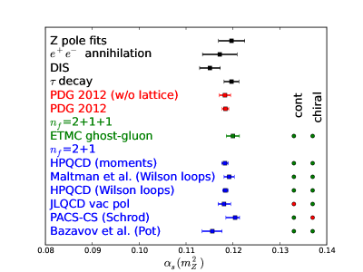
Figure 1: Summary of $\alpha_{s}$ measurements from lattice QCD and summaries from other methods.

In table 2 I summarize the different methods of extracting $\alpha_{s}$ from lattice QCD and the summary of results are in figure 1. The color coding is different to the quark mass summary plots and is explained in section 1. I also include the PDG summary values [1] for different non-lattice methods for determining $\alpha_{s}$.

The final summary for $\alpha_{s}(M_{Z}^{2})$ from the PDG [1] is 0.1184(7). If the lattice results were not included in the average the result $\alpha_{s}(M_{Z}^{2})$ = 0.1183(12) was obtained, so the lattice results for $\alpha_{s}$ are consistent with other methods, but they are important for the final error. One of the goals of running a linear collider at the Z peak (the GigaZ option [24]) was to measure $\alpha_{s}(M_{Z}^{2})$ to an accuracy of 0.001, which is already achieved if the PDG error is not underestimated.

Many people worry that the error for $\alpha_{s}$ is dominated by the results from lattice QCD, and one reviewer [25] of $\alpha_{s}$ measurements reported, without any reasons, that he didn’t believe the error on the lattice results. The lattice calculation using Wilson loop by Maltman et al. [26] was partly motivated to check an earlier calculation of $\alpha_{s}$ by the HPQCD collaboration. The mini-proceedings of a recent workshop [27]. on $\alpha_{s}$ provide a useful summary of the views and results of the experts.

From table 2 the lowest scale used to determine $\alpha_{s}$ is 0.8 GeV. There have been speculations that the coupling will evolve to a constant for low scales (for example [28]). There have been some lattice QCD calculations to investigate the coupling defined in Eq. 6 for small momentum. The motivation for these calculation is to test confinement models and different solutions of Schwinger-Dyson equations.

Momentum on the lattice is quantized in units of $p=\frac{2\pi}{L}$ for a box side $L$, so large spatial volumes (for example ($\mbox{16 fm})^{4}$ in [29] ) are required to reach small momentum. The results of Bogolubsky et al. [29] (see figure 5 of  [29]) shows that the coupling defined in Eq. 6 goes to zero for small momentum. This corresponds to the “decoupling solution” of Schwinger-Dyson equation. The requirement for large volumes means that the lattice QCD calculations are done in quenched QCD ($n_{f}$=0) with coarse lattice spacing with no continuum limit.

Currently there many lattice calculations which are studying the evolution of coupling in QCD like theories with a large number of sea quarks or quarks in a adjoint representation to help BSM model builders using strongly interacting theories (see [30] for a recent review).

3.1 $\alpha_{s}$ and the unification of couplings

The error on the value of $\alpha_{s}$ is the biggest error on the the unification of the three standard model gauge couplings. Although the inclusion of additional degrees of freedom from SUSY theories improves the unification of all three coupling at a single scale, the agreement is not perfect.

Some groups have tried to use the unification of couplings as a way to discriminate between different SUSY models. For example King et al. [31] find a more accurate unification of couplings in their exceptional super-symmetric standard model, than with the MSSM. There is even work with the unification of couplings in technicolor models [32]. One of the goals of the linear collider running as the GigaZ option [24] (as a Z factory) was to measure $\alpha_{s}$ more accurately to test unification. A report [33] for the proposed Large Hadron Electron Collider estimates that it may be possible to calculate $\alpha_{s}$ to an accuracy of 0.11 % from DIS and mention testing coupling unification as motivation. The status of the coupling unification of the couplings is reviewed by Raby in the GUT review in the PDG [1].

Table 3: $\beta$ functions for standard model and MSSM. $n_{g}$ generations and $n_{h}$ Higgs doublets.

$b_{i}$	Standard model	MSSM
$b_{3}$	11 - $\frac{4}{3}n_{g}$	9 - 2 $n_{g}$
$b_{2}$	$\frac{22}{3}$ - $\frac{4}{3}n_{g}$ - $\frac{1}{6}n_{h}$	6 - 2 $n_{g}$ - $\frac{1}{2}n_{h}$
$b_{1}$	- $\frac{4}{3}n_{g}$ - $\frac{1}{10}n_{h}$	-2 $n_{g}$ - $\frac{3}{10}n_{h}$

As an illustrative example I use one loop evolution equations of the QCD and electroweak couplings as a function of the scale $Q$. I essentially follow the example in the text book [34] (see also Peskin [35].)

$$1/\alpha_{i}(Q)=1/\alpha_{i}(M_{Z})+\frac{b_{i}}{2\pi}\log(Q/M_{Z})$$ (10)

The first two couplings are defined by

$$\alpha_{2}^{-1} = \alpha_{em}^{-1}\sin^{2}(\theta_{W})$$ (11)

$$\alpha_{1}^{-1} = \frac{3}{5}\alpha_{2}^{-1}\cot^{2}(\theta_{W})$$ (12)

where $\alpha_{em}$ is the QED coupling and $\theta_{W}$ is the weak mixing angle. The third coupling ($\alpha_{3}$) is the QCD coupling $\alpha_{s}$. The explicit values for $b_{1}$, $b_{2}$, and $b_{3}$ are in table 3 in terms of the number of Higgs bosons and generations.

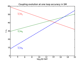
Figure 2: Coupling unification in SM

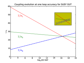
Figure 3: Coupling unification in MSSM

In figure 3 I show the running of the three couplings in the standard model and in figure 3, I show the equivalent plot for the MSSM, including the 1$\sigma$ error band from $\alpha_{s}$ and the region around unification scale magnified. It is clear that unification in the MSSM is better than for the standard model, but that the unification is not exact in the MSSM. I have not investigated using two loop evolution equations, because that involves threshold effects for new particles. References to more detailed calculations were discussed above [31, 32, 24].

Once some evidence for BSM particles is found and or proton decay is observed, then the error on $\alpha_{s}$ will be an important factor for tests of coupling unification, and thus help to explore the physics at the unification scale.

The value of $\alpha_{s}$ is also important for the stability of the Higgs potential [36].

4 The mass of the charm quark from lattice QCD

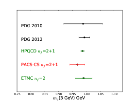
Figure 4: Mass of the charm quark.

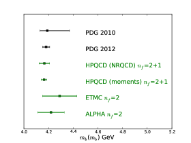
Figure 5: Mass of the bottom quark.

The main complication for including the charm quark in lattice QCD calculations is that the size of the charm mass in lattice units is not small, which can cause problems with the continuum extrapolation. Standard effective field theories such as NRQCD or HQET are not useful for charm, but a lattice effective field theory developed by the FNAL group and others is commonly used.

I summarize recent results for the mass of the charm quark in figure 5. The HPQCD collaboration [15] used the moments method to compute $m_{c}(\mbox{3 GeV})$. The ETM collaboration [37] included 4 lattice spacings and the renormalization of the quark mass was done with the Rome-Southampton technique. The PACS-CS collaboration [38] have computed the mass of the charm quark at single lattice spacing $a^{-1}=2.194(10)$ GeV, but using the physical pion mass after re-weighting a lattice QCD calculation with pion mass of of 152(6) MeV. The renormalisation was done by a non-perturbative method for the massless factor and one loop perturbation theory for the massive renormalization contribution.

5 The mass of the bottom quark from lattice QCD.

Until very recently the mass of the bottom quark was too big in lattice units for standard lattice actions to be used, hence the majority of lattice QCD calculations used an effective field theory, such as NRQCD or static QCD. In figure 5 I show a summary plot for the mass of the bottom quark from lattice QCD.

The HPQCD collaboration has recently published [10] a result for $m_{b}(m_{b})$ using Non-relativistic QCD for the bottom quark. The $O(v^{4})$ improved Symanzik action NRQCD action was used. The basic idea is to compute the binding energy of a heavy-light or heavy meson. The mass of the bottom quark [10] in the $\overline{MS}$ scheme $m_{b}(\mu)^{\overline{MS}}$ is extracted from

$$m_{b}(\mu)^{\overline{MS}}=\frac{1}{2Z_{M}(\mu)}\left(M^{expt}_{\Upsilon}-a^{-1}(aE_{sim}-2aE_{0})\right)$$ (13)

where $E_{sim}$ is the measured binding energy in the lattice calculation, $E_{0}$ is a lattice perturbative factor, $M^{expt}_{\Upsilon}$ is the experimental mass of the Upsilon meson and $Z_{M}(\mu)$ is the perturbative matching factor between the pole mass and the $\overline{MS}$ mass in continuum perturbation theory. The final perturbative expression for $m_{b}(\mu)^{\overline{MS}}$ should be free of renormalon ambiguities, because of cancellation between the series for $Z_{M}(\mu)$ and $E_{0}$. A value for $m_{b}$ was also extracted from the $B_{s}$ mass.

The lattice NRQCD action is complicated, so it is difficult to do higher order calculations of $E_{0}$ using lattice perturbation theory, instead a mixed approach was taken. The quenched diagrams were done by doing the numerical calculation with very fine lattice spacings. The $\alpha_{s}^{2}n_{f}$ contributions were obtained by directly computing the 4 Feynman graphs in lattice perturbation theory. The numerical lattice QCD calculation used two ensembles with lattice spacings: 0.09 and 0.12fm.

In the past the static (infinite mass) limit effective field theory has been used to compute the mass of the bottom quark. The ALPHA collaboration developed an elegant method to compute the $1/M_{Q}$ corrections to the static limit with a numerical method [39].

The ETM collaboration [40, 41] has developed a technique to take multiple ratios of the meson mass divided by the quark pole mass (motivated by HQET). This allowed an extrapolation of their data up to the bottom quark mass.

The HPQCD collaboration has developed the relativistic HISQ action [42] (with no $O(a^{2})$ tree lattice spacings corrections) The MILC collaboration [43] have generated gauge configurations with the smallest lattice spacing of 0.045 fm. These two developments allowed bare quark masses close to the physical bottom mass to be used in the calculation with the relativistic action. The moments method was used to compute $m_{b}(m_{b})$ in a similar manner to calculation of the mass of the charm quark in section 4. There was also a cross-check on the moments calculation by taking ratios of $m_{b}/m_{c}$ from the quark mass used in the action.

6 A review of lattice reviews

There are a number of groups which review lattice QCD calculations of the masses of quark masses. There is a review section on quark masses in the PDG written by Sachrajda and Manohar. The FLAG group have provided a comprehensive review of the light quark masses [7]. There is also a group of three people called the Lattice averaging group [44] (http://latticeaverages.org/) which provide averages of various quantities, including the light quark masses. FLAG joined by the lattice averaging group, are planning to expand their review [45] to include the charm and bottom quark masses and $\alpha_{s}$.

In the past there have been reviews of quark masses at either the annual lattice conference or other conferences. For example Heitger [46] and Davies [47].

The quark masses are usually quoted at standard scales, such as 2, 3 GeV or the mass of the bottom quark, but these may be too small for BSM model building. So there are summary tables of quark masses at 1 TeV and higher [48], which mostly use as input the quark masses from the PDG [1].

One important issue is how to correctly average the lattice QCD results. Most lattice results quote errors that are a mixture of statistical or systematic errors. The PDG [1] use a simple weighted mean without including any correlations to average their data. The errors are increased if $\chi^{2}/dof>1$. The are a number of possible causes for correlations between the results from different lattice QCD calculations. For example, some lattice calculations use the same gauge configurations, but use different valence actions. Sometimes an unphysical quantity such as $r_{1}$ calibrated by another lattice QCD calculation is used by a number of different calculations, which partially correlate the errors. The lattice averaging group [44] have started to compute lattice QCD averages with correlations (using the formalism in [49]). FLAG [7] argue that their error estimates are conservative enough to not require the use of correlations.

A particularly important issue is what results to include. For example the lattice averaging group will include the results presented at conferences, if in their judgement the error analysis is reliable, but FLAG only include results published in journals.

7 The mass of the strange and light quarks

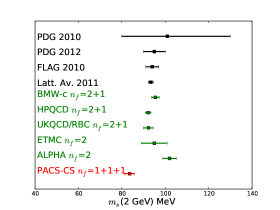
Figure 6: Mass of the strange quark.

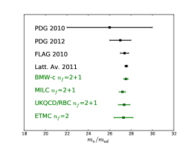
Figure 7: Summary of $\frac{m_{s}}{m_{ud}}$

I plot a summary of some recent lattice QCD calculations of the mass of the strange quark in figure 7 . I plot the ratio of the quark masses $m_{s}$ to $m_{ud}$ (where $m_{ud}=\frac{m_{u}+m_{d}}{2}$) from some recent lattice QCD calculations in figure 7. The FLAG group [7] has reviewed the determination of the masses of light quarks, but does not include the more recent results [50, 51, 52].

BMW-c have computed the mass of the strange quark [53] from a lattice QCD calculation with 2+1 flavors of sea quarks. The analysis included 5 lattice spacings, three of which included ensembles at the physical pion mass. The Rome-Southampton technique was used to compute the lattice part of the renormalisation numerically [8]. The UKQCD/RBC collaboration have recently reported [52] the mass of the strange quark using a similar technique to that used by BMW-c, but using heavier pion masses, different lattice actions, and only two lattice spacings. The ETM collaboration also used the Rome-Southampton technique to renormalise their quark masses [37].

The HPQCD collaboration [54] computed the mass of the strange quark by calculating the $m_{c}/m_{s}$ ratio in the continuum limit, and using $m_{c}$ computed with the moments method [14, 15].

8 Including QED and isospin violation in lattice calculations

Currently the majority of lattice QCD calculations only include $n_{f}$ = 2, 2+1 or 2+1+1 flavors of sea quarks. To extract the individual up or down quark masses requires QED and isospin violation from effective field theory to be added to the results of these calculations by hand (see [45] for a review).

There is a lot of development of lattice calculations [55, 56, 57, 50] which directly include isospin and QED. There are additional challenges to lattice QCD calculations which include the dynamics of 1+1+1 sea quarks and the dynamics of QED. For example including QED makes the calculations more noisy and the renormalisation is more complicated. The long range nature of QED may cause additional finite size effects [58]. The calculation of the correlators for the $\pi^{0}$ require the calculation of disconnected diagrams when $m_{u}\neq m_{d}$.

Including quenched QED in lattice QCD calculations is done by multiplying the U(1) field, generated by a separate lattice calculation, into the QCD gauge fields. The RBC collaboration [56] are using re-weighting to move from a lattice QCD calculation with 2+1 sea quarks and no QED to one which includes the QED dynamics in the sea. More ambitiously the PACS-CS collaboration [50] are using re-weighting to move from a 2+1 lattice QCD calculation to a 1+1+1+QED calculation. The RM123 collaboration [59, 60] have developed a formulation that measures additional correlators, based on an expansion in $m_{u}-m_{d}$ and including quenched QED [60].

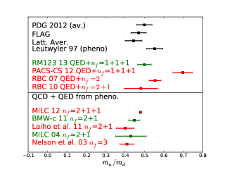
Figure 8: Summary of recent values for $m_{u}/m_{d}$

I summarize in figure 8 the values of the ratio of $m_{u}/m_{d}$ from lattice QCD and non-lattice methods included in the PDG summary of $m_{u}/m_{d}$. I include results from review groups [45, 44, 1], lattice calculations which include the dynamics of QED in someway [61, 55, 60, 50], and lattice calculations which include the QED from phenomenology [62, 63, 3, 64, 65]. The PACS-CS result for $m_{u}/m_{d}$ was from a calculation at only one lattice spacing [50]. I am disappointed that the errors on $m_{u}/m_{d}$ have not been reduced by much since the result by MILC in 2004 [64].

8.1 Testing textures with quark masses

Ideally I would like to understand why the CKM matrix is diagonally dominant and the hierarchy of quark masses. Unfortunately, currently there are no compelling BSM models which make definite and falsifiable predictions for the masses of the quarks. There has been a long history [66] of looking for patterns in the CKM matrix elements and quark masses from textures. This is numerology, but may give some hints. There are reviews of textures [67, 68, 69]. I hope that the reduced errors on the masses of the quarks from lattice QCD calculations will help constrain some of the proposed relations between CKM matrix elements and the masses of the quarks.

As one example, I use lattice QCD results to test one proposed connection between the $V_{us}$ CKM matrix elements and the massess of the up and strange quarks, from the model by Chkareuli and Froggatt [70] (other relations from Ref. [70] were tested in Ref. [71].)

$$V_{us}\sim\sqrt{\frac{m_{d}}{m_{s}}}=\sqrt{\frac{2}{(1+m_{u}/m_{d})m_{s}/m_{ud}}}$$ (14)

There are possible corrections to Eq. 14 which can be tested with more accurate values of the quark masses. The relation in Eq. 14 is not scale invariant, because of the scale evolution of $V_{us}$, so may only hold at specific scale, such as the unification scale.

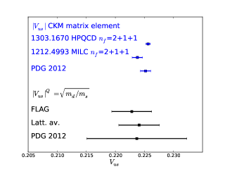
Figure 9: Testing $V_{us}\sim\sqrt{\frac{m_{d}}{m_{s}}}$

In figure 9 I compare the right and left hand sides of Eq. 14 with recent results for quark masses [7, 44, 1] and the $V_{us}$ CKM matrix element [7, 72, 73]. The errors on the quark masses must be further reduced to test the relation in 14. The error $m_{u}/m_{d}$ needs to be of the order of the preliminary result quoted by the MILC collaboration [62] to produce an error with a similar size to that of $V_{us}$ in equation 14.

9 Anthropic constraints on the quark masees

If you don’t like even trying to use textures to “explain” the CKM matrix and masses of the quarks, there is a much worse possibility. Although the LHC did find the Higgs boson, it has so far not found any evidence for BSM particles, hence it could be that the standard model of particle physics is all there is and we will never understand the values of the quark masses.

At the lattice 2002 conference Wilczek briefly reviewed [74] various anthropic principles and suggested that the lattice QCD community investigate them. The subject of anthropics comes with a lot of philosophical baggage (such as those associated with the current multi-verse mania) that I will just ignore. However questions such as by how much can the masses of the light quarks be varied before deuterium is unbound is a well defined (and hence scientific) question. Lattice QCD can map out the quark mass dependence of physical quantities, so should be able to contribute. Here I will briefly review what has been done for constraints on the sum of the light quark masses ($m_{ud}$). The are also constraints on the difference of the mass of the up and down quarks which I do not discuss [75] (see Ref. [76] for a recent lattice calculation.)

The properties of the lighter nuclei can be obtained from solving an effective field theory or a model, of protons and neutrons interacting [77, 78, 79]. The parameters of the effective field theory can be extracted from experiment or lattice QCD calculations. Examples of the parameters of the effective field theory are the nucleon axial charge ($g_{A}$) and nucleon-nucleon scattering lengths. The basic idea is that the effective field theory computes the binding energy of nuclei in terms of hadronic degrees of freedom. The dependence of the nucleon, pion and other quantities on the quark masses is used to compute the sensitivity of the nuclei binding energies on the quark masses.

For example Donoghue and Damour [75] found the constraint

$$\frac{m_{ud}}{(m_{ud})_{\mbox{phys}}}<1.64$$

at 95% confidence level, from the existence of nuclear binding. Jaffe et al. [80] have also investigated the effect of varying the quark masses on producing the stable nuclei required to make organic chemistry possible.

Epelbaum et al. [81] have studied the light quark mass dependence of the binding energy of the Hoyle state ${}^{12}C$. The production of carbon and oxygen in red giant stars requires this state to exist. From their calculation they find that the production of carbon and oxygen via the Hoyle state is stable for a 2% change in the light quark masses.

There are also tight constraints on the quark masses form from Big Bang nucleosynthesis [82, 83]. For example, Berengut et al. [83] find $\frac{\delta m_{ud}}{m_{ud}}<0.02\pm 0.04$ for nucleosynthesis.

9.1 Condensates from lattice QCD

Lattice QCD calculations also provide values for non-perturbative quantities which are useful input to sum rule calculations, and other formalisms which are used to solve QCD. There have been a large number of lattice QCD calculations of the chiral condensate. See Cichy et al. [84] for a recent calculation of the chiral condensate and a summary of the results of other calculations. The gluon condensate $\langle\frac{\alpha}{\pi}GG\rangle$ has recently been estimated from the plaquette [85] using lattice QCD.

In the last year the ratio of strange to light condensates has been computed using lattice QCD [86]. The key problem is that there is a $1/a^{2}$ divergence in the condensate with massive quarks, which must be subtracted off. The ratio of the strange to light quark condensate was found to be 1.08(16) [86].

10 Conclusions

Lattice QCD calculations have recently produced accurate results for quark masses and the strong coupling with errors at the % level. These results required lattice QCD calculations with controlled continuum extrapolations, pion masses below 300 MeV (and even in some cases below the physical pion mass) and the renormalisation of the quark masses beyond one loop level.

It is important to have additional results for quark masses and the QCD coupling from other discritization of the QCD action, and in particular results from lattice QCD calculations which include the dynamics of the charm quark in the sea (there are at least two in progress).

This work is supported by SFB-TR 55.

References

- [1] Particle Data Group, J. Beringer et al., Phys.Rev. D86, 010001 (2012).
- [2] A. Bazavov et al., Phys.Rev. D87, 054505 (2013), arXiv:1212.4768.
- [3] S. Durr et al., JHEP 1108, 148 (2011), arXiv:1011.2711.
- [4] C. Hoelbling, PoS LATTICE2010, 011 (2010), arXiv:1102.0410.
- [5] S. Durr et al., Science 322, 1224 (2008), arXiv:0906.3599.
- [6] E. Gregory et al., Phys.Rev.Lett. 104, 022001 (2010), arXiv:0909.4462.
- [7] G. Colangelo et al., Eur.Phys.J. C71, 1695 (2011), arXiv:1011.4408.
- [8] G. Martinelli et al., Nucl.Phys. B445, 81 (1995), arXiv:hep-lat/9411010.
- [9] K. Jansen et al., Phys.Lett. B372, 275 (1996), arXiv:hep-lat/9512009.
- [10] A. Lee et al., Phys. Rev. D 87, 074018 (2013), arXiv:1302.3739.
- [11] C. Davies et al., Phys.Rev. D78, 114507 (2008), arXiv:0807.1687.
- [12] A. Sternbeck et al., PoS LATTICE2012, 243 (2012), arXiv:1212.2039.
- [13] K. Wong et al., Phys.Rev. D73, 094512 (2006), arXiv:hep-lat/0512012.
- [14] I. Allison et al., Phys.Rev. D78, 054513 (2008), arXiv:0805.2999.
- [15] C. McNeile et al., Phys.Rev. D82, 034512 (2010), arXiv:1004.4285.
- [16] E. Shintani et al., Phys.Rev. D82, 074505 (2010), arXiv:1002.0371.
- [17] A. Bazavov et al., Phys.Rev. D86, 114031 (2012), arXiv:1205.6155.
- [18] A. Smirnov et al., Phys.Rev.Lett. 104, 112002 (2010), arXiv:0911.4742.
- [19] C. Anzai et al., Phys.Rev.Lett. 104, 112003 (2010), arXiv:0911.4335.
- [20] B. Blossier et al., Phys.Rev.Lett. 108, 262002 (2012), arXiv:1201.5770.
- [21] A. Sternbeck et al., PoS LAT2007, 256 (2007), arXiv:0710.2965.
- [22] F. Tekin et al., Nucl.Phys. B840, 114 (2010), arXiv:1006.0672.
- [23] S. Aoki et al., JHEP 0910, 053 (2009), arXiv:0906.3906.
- [24] B. Allanach et al., (2004), arXiv:hep-ph/0403133.
- [25] G. Altarelli, (2013), arXiv:1303.6065.
- [26] K. Maltman et al., Phys.Rev. D78, 114504 (2008), arXiv:0807.2020.
- [27] S. Bethke et al., (2011), arXiv:1110.0016.
- [28] B. Ermolaev, M. Greco, and S. Troyan, Eur.Phys.J.Plus 128, 34 (2013), arXiv:1209.0564.
- [29] I. Bogolubsky, E. Ilgenfritz, M. Muller-Preussker, and A. Sternbeck, Phys.Lett. B676, 69 (2009), arXiv:0901.0736.
- [30] J. Giedt, PoS LATTICE2012, 006 (2012).
- [31] S. King et al., Phys.Lett. B650, 57 (2007), arXiv:hep-ph/0701064.
- [32] S. B. Gudnason et al., Phys.Rev. D76, 015005 (2007), arXiv:hep-ph/0612230.
- [33] LHeC Study Group, J. Abelleira Fernandez et al., J.Phys. G39, 075001 (2012), arXiv:1206.2913.
- [34] I. Aitchison, (2007).
- [35] M. E. Peskin, (1997), arXiv:hep-ph/9705479.
- [36] J. Elias-Miro et al., Phys.Lett. B709, 222 (2012), arXiv:1112.3022.
- [37] B. Blossier et al., Phys.Rev. D82, 114513 (2010), arXiv:1010.3659.
- [38] Y. Namekawa et al., Phys.Rev. D84, 074505 (2011), arXiv:1104.4600.
- [39] F. Bernardoni et al., Nucl.Phys.Proc.Suppl. 234, 181 (2013), arXiv:1210.6524.
- [40] B. Blossier et al., JHEP 1004, 049 (2010), arXiv:0909.3187.
- [41] P. Dimopoulos et al., JHEP 1201, 046 (2012), arXiv:1107.1441.
- [42] E. Follana et al., Phys.Rev. D75, 054502 (2007), arXiv:hep-lat/0610092.
- [43] A. Bazavov et al., Rev.Mod.Phys. 82, 1349 (2010), arXiv:0903.3598.
- [44] J. Laiho et al., Phys.Rev. D81, 034503 (2010), arXiv:0910.2928.
- [45] G. Colangelo, PoS LATTICE2012, 021 (2012).
- [46] J. Heitger, Nucl.Phys.Proc.Suppl. 181+182, 156 (2008), arXiv:0901.1088.
- [47] C. Davies, (2013), arXiv:1301.7202.
- [48] Z. Xing et al., Phys.Rev. D77, 113016 (2008), arXiv:0712.1419.
- [49] M. Schmelling, Phys.Scripta 51, 676 (1995).
- [50] S. Aoki et al., Phys.Rev. D86, 034507 (2012), arXiv:1205.2961.
- [51] P. Fritzsch et al., Nucl.Phys. B865, 397 (2012), arXiv:1205.5380.
- [52] R. Arthur et al., (2012), arXiv:1208.4412.
- [53] S. Durr et al., Phys.Lett. B701, 265 (2011), arXiv:1011.2403.
- [54] C. Davies et al., Phys.Rev.Lett. 104, 132003 (2010), arXiv:0910.3102.
- [55] T. Blum et al., Phys.Rev. D82, 094508 (2010), arXiv:1006.1311.
- [56] T. Ishikawa et al., Phys.Rev.Lett. 109, 072002 (2012), arXiv:1202.6018.
- [57] A. Portelli et al., PoS LATTICE2011, 136 (2011), arXiv:1201.2787.
- [58] M. Hayakawa et al., Prog.Theor.Phys. 120, 413 (2008), arXiv:0804.2044.
- [59] G. de Divitiis et al., JHEP 1204, 124 (2012), arXiv:1110.6294.
- [60] G. de Divitiis et al., (2013), arXiv:1303.4896.
- [61] T. Blum et al., Phys.Rev. D76, 114508 (2007), arXiv:0708.0484.
- [62] A. Bazavov et al., PoS LATTICE2012, 159 (2012), arXiv:1210.8431.
- [63] J. Laiho et al., PoS LATTICE2011, 293 (2011), arXiv:1112.4861.
- [64] C. Aubin et al., Phys.Rev. D70, 114501 (2004), arXiv:hep-lat/0407028.
- [65] D. R. Nelson et al., Phys.Rev.Lett. 90, 021601 (2003), arXiv:hep-lat/0112029.
- [66] H. Fritzsch, Phys.Lett. B73, 317 (1978).
- [67] H. Fritzsch et al., Prog.Part.Nucl.Phys. 45, 1 (2000), arXiv:hep-ph/9912358.
- [68] K. Babu, p. 49 (2009), arXiv:0910.2948.
- [69] M. Gupta and G. Ahuja, Int. Jour. Mod. Phys. A, 27,, 1230033 (2012), arXiv:1302.4823.
- [70] J. Chkareuli et al., Phys.Lett. B450, 158 (1999), arXiv:hep-ph/9812499.
- [71] C. McNeile, (2010), arXiv:1004.4985.
- [72] A. Bazavov et al., (2013), arXiv:1301.5855.
- [73] R. Dowdall et al., (2013), arXiv:1303.1670.
- [74] F. Wilczek, Nucl.Phys.Proc.Suppl. 119, 3 (2003), arXiv:hep-lat/0212041.
- [75] T. Damour and J. F. Donoghue, Phys.Rev. D78, 014014 (2008), arXiv:0712.2968.
- [76] S. Borsanyi et al., (2013), arXiv:1306.2287.
- [77] D. Lee, Prog.Part.Nucl.Phys. 63, 117 (2009), arXiv:0804.3501.
- [78] M. Savage, Prog.Part.Nucl.Phys. 67, 140 (2012), arXiv:1110.5943.
- [79] E. Epelbaum, (2013), arXiv:1302.3241.
- [80] R. L. Jaffe, A. Jenkins, and I. Kimchi, Phys.Rev. D79, 065014 (2009), arXiv:0809.1647.
- [81] E. Epelbaum, H. Krebs, T. A. Lahde, D. Lee, and U.-G. Meissner, Phys.Rev.Lett. 110, 112502 (2013), arXiv:1212.4181.
- [82] P. F. Bedaque, T. Luu, and L. Platter, Phys.Rev. C83, 045803 (2011), arXiv:1012.3840.
- [83] J. Berengut et al., Phys.Rev. D87, 085018 (2013), arXiv:1301.1738.
- [84] K. Cichy et al., (2013), arXiv:1303.1954.
- [85] R. Horsley et al., Phys.Rev. D86, 054502 (2012), arXiv:1205.1659.
- [86] C. McNeile et al., Phys.Rev. D87, 034503 (2013), arXiv:1211.6577.