Effective preparation and collisional decay of atomic condensate in excited bands of an optical lattice

Abstract

We present a method for the effective preparation of a Bose-Einstein condensate (BEC) into the excited bands of an optical lattice via a standing-wave pulse sequence. With our method, the BEC can be prepared in either a single Bloch state in a excited-band, or a coherent superposition of states in different bands. Our scheme is experimentally demonstrated by preparing a ⁸⁷Rb BEC into the $d$-band and the superposition of $s$- and $d$-band states of a one-dimensional optical lattice, within a few tens of microseconds. We further measure the decay of the BEC in the $d$-band state, and carry an analytical calculation for the collisional decay of atoms in the excited-band states. Our theoretical and experimental results consist well.

.

I introduction

Ultracold atomic gases in optical lattices have various applications in many fields, including the quantum simulation of many-body systems and the realization of quantum computation and high-precision atomic clock  RMP06 ; RMP08 ; RMP11 . So far most of the experiments have been implemented in ground bands ($s$-bands) of optical lattices. Recently, ultracold gases in the excited bands of optical lattices attract many attentions. It is proposed that many interesting many-body phenomena, e.g., supersolid quantum phases in cubic lattices Scarola , quantum stripe ordering in triangular lattices Wu , orbital degeneracy Lewenstein can appear in the ultracold atoms in the excited-band states. Nevertheless, the $d$- and $f$-band physics in optical lattices have remained experimentally unexplored, except the bipartite square optical lattice M .

A common concern for the research of excited-band physics of ultracold gas in an optical lattice is how to rapidly load the atoms into the high energy bands without excitation or heating. So far several experimental techniques have been developed for preparing ultracold atoms in the high energy bands. These techniques include: (i) the coherent manipulation of vibrational bands by stimulated Raman transitions Muller , (ii) using a moving lattice to load a Bose-Einstein condensate (BEC) into a excited-band Browaeys , (iii) the population swapping technique for selectively exciting the atoms into the $p$-band Wirth1 or $f$-band M of a bipartite square optical lattice. It is pointed out that, these approaches are designed to transfer the atoms from the $s$-band to the excited bands. Namely, to create an ultracold gas in the excited band of the optical lattice with these approaches, one needs to first load the atoms into the $s$-band. With the widely-used adiabatic loading approach, such a process takes several tens of milliseconds.

In this paper, we develop a method for effective preparation of a weakly-interacting Bose-Einstein condensate (BEC) in the high energy bands of an optical lattice. This scheme is based on our previous work for the rapid loading of BEC into the ground state of an optical lattice via a standing-wave laser pulse sequence Liu ; Xiong . With our method, the BEC can be directly transferred from the ground state of the weak harmonic trap into the excited band of the optical lattice with a non-adiabatic process, which can normally be completed within several tens of microseconds. Furthermore, in our scheme the BEC can be prepared in either a single excited-band Bloch state or a coherent superposition of Bloch states in different bands with the same quasi-momentum. As a demonstration, we experimentally realize the effective preparation of a ⁸⁷Rb BEC into a $d$-band state, and the coherent superposition of $d$-band and $s$-band states of an one-dimensional (1D) optical lattice. The effectiveness of our approach is further verified by the observations of the atomic Rabi oscillations between states with different single-atom momentum. As shown below, the fidelities of the preparation process in our experiments are as high as 97%-99%.

As an application of our method, we experimentally investigate the decay process of the ⁸⁷Rb BEC, which is rapidly loaded in the $d$-band of the 1D optical lattice. It is well known that, when the ultracold atoms are prepared in the excited-band state of an optical lattice, they can decay to the states in the lower bands via inter-atomic collision. For the ultracold gas prepared around the lowest-energy points of high energy bands, the lifetime of the gas is mainly determined by the collisional decay. Such a decay process was experimentally observed by N. Katz et al. in a moving optical lattice Katz and theoretically studied with a perturbative calculation by the same authors Katz . Nevertheless, to the best of our knowledge, there is still lack of a first-principle calculation for the collisional-decay rate. In this paper, based on the scattering theory, we provide a first-principle calculation for the collisional-decay process of ultracold gases in the excited bands, and obtain the analytical expression of the decay rate. We compare our theoretical result and the experimental observations, and find great consistency.

The remainder of this manuscript is organized as follows. In Sec. II, we introduce our method for effective preparation of BEC in the excited-band states. Our experiment for the preparation of the BEC of ⁸⁷Rb atoms is shown in Sec. III. In Sec. IV we analytically calculate the rate of the collisional decay of atoms in the $d$-band state, and compare our result with the experimental observations. The main results are summarized and discussed in Sec. V, while some details of our calculations are given in the appendix.

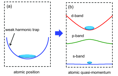
Figure 1: (Color online) The system before and after the preparation process. (a) Before the process, the BEC is confined in a weak harmonic trap. (b) After the preparation process, an optical lattice is turned on and the atoms in the condensate are transferred into a single quasimomentum state, or the superposition of quasimomentum states in different energy bands.

II Approach for effective preparation of BEC in excited bands

Now we introduce our approach for rapidly preparing a BEC in the excited bands of an optical lattice. For simplicity, in this section we only consider the case with 1D optical lattice. Our method introduced here can be straightforwardly generalized to the systems with two- or three-dimensional lattice.

In the ultracold gas of single-component bosonic atoms, a 1D optical lattice can be created by two counter-propagating laser beams. In the presence of the optical lattice, the single-atom Hamiltonian in the $x$-direction is given by $(\hbar=1)$

$$H_{x}=\frac{p_{x}^{2}}{2m}+V_{0}\cos^{2}\left(\frac{x}{a}\pi\right),$$ (1)

with $m$ and $p_{x}$ the single-atom mass and momentum in the $x$-direction, respectively. Here $V_{0}$ is the depth of the optical lattice and $a$ is the lattice constant. According to the Bloch’s theorem, the eigen-state of $H_{x}$ can be expressed as $|n,q\rangle\equiv u_{n,q}\left(x\right)e^{iqx}/\sqrt{2\pi}$, with $n=s,p,d...$ the index of the energy band, and $q\in[-\pi/a,\pi/a)$ the quasi-momentum. Here the periodic Bloch function $u_{n,q}\left(x\right)$ satisfies $u_{n,q}\left(x\right)=u_{n,q}\left(x+a\right).$ Using this property, it can be easily proved that Bloch state $|n,q\rangle$ is the superposition of the plane waves $e^{ikx}/\sqrt{2\pi}$, with $k=q+2j\pi/a$ $(j=0,\pm 1,\pm 2,....)$. Namely, $|n,q\rangle$ can be re-expressed as

$$|n,q\rangle=\sum_{j=-\infty}^{+\infty}C_{nj}(q)|p_{x}=q+2j\pi/a\rangle,$$ (2)

where $|p_{x}=k\rangle\equiv e^{ikx}/\sqrt{2\pi}$ is the eigen-state of $p_{x}$ with eigen-value $k$, and $C_{nj}$ is the superposition coefficient.

As shown in Fig. 1, we suppose that before the preparation process, there is no optical lattice in our system, and the atoms are condensed in the single-atom ground state of the weak harmonic trap. We further approximate such a state to be $|p_{x}=0\rangle$ with zero momentum. Our purpose is to prepare the condensed atom in a given superposition state

$$|\Psi_{a}\rangle=\sum_{n}f_{n}|n,q_{0}\rangle.$$ (3)

According to Eq. (2), $|\Psi_{a}\rangle$ can be expressed as the superposition of the states $|p_{x}=q_{0}+2j\pi/a\rangle$, i.e., we have

$$|\Psi_{a}\rangle=\sum_{j=-\infty}^{+\infty}d_{j}|p_{x}=q_{0}+2j\pi/a\rangle,$$ (4)

with $d_{j}=\sum_{n}f_{n}C_{nj}(q_{0})$.

We first consider a simple case where $|\Psi_{a}\rangle$ is the superposition of the zero-quasi-momentum Bloch states in the “even bands”, i.e., the case with $q_{0}=0$ and $f_{p,f,h,...}=0$. In that case, with our method the preparation process is accomplished via alternating cycles of switching on (duty cycle) and off (off-duty cycle) the optical lattice. In these duty cycles, the atom experiences spatial potential $V_{0}\cos^{2}\left(x\pi/a\right)$. Such a potential can induce the transition between the states $|p_{x}=2j\pi/a\rangle$ with different values of $j$. In the off-duty cycle, the atom is governed by the free-Hamiltonian $p_{x}^{2}/(2m)$. Thus, although there is no transition between different eigen-states of $p_{x}$, these states can gain different phase factors. Therefore, when the duty and off-duty cycles are alternately applied to the atoms at state $|p_{x}=0\rangle$, the atoms can be prepared to a superposition state of $|p_{x}=2j\pi/a\rangle$, i.e., a state with the form in Eq. (4). It is pointed out that, since the initial atomic momentum is zero and the quasi-momentum is conserved in both of the two cycles, in the preparation process the atomic state can only be the superposition of the zero-quasi-momentum states in different energy bands. Finally, when all the duty and off-duty cycles are completed, we instantaneously switch on the optical lattice, and then the atoms are loaded in the optical lattice.

The above preparation approach can be mathematically described as follows. We assume the preparation process includes $N_{C}$ duty cycles and $N_{C}$ off-duty cycles, and the duration of the $l$th duty and off-duty cycle is $\tau_{l}$ and $\tau_{l}^{\prime}$, respectively. Thus, after the preparation process, the atomic state would be

$$|\Psi_{L}\rangle\equiv\prod_{l}e^{-i\frac{p_{x}^{2}}{2m}\tau_{l}^{\prime}}e^{-i[\frac{p_{x}^{2}}{2m}+V_{0}\cos^{2}\left(x\frac{\pi}{a}\right)]\tau_{l}}|p_{x}=0\rangle.$$ (5)

Therefore, for a given target state $|\Psi_{a}\rangle$, the parameters $N_{C}$ and $\{\tau_{l},\tau_{l}^{\prime}\}$ can be determined via maximizing the fidelity

$$F=\left|\langle\Psi_{L}|\Psi_{a}\rangle\right|^{2}.$$ (6)

It is apparent that the value $1-F$ just describes the difference between the realistic atomic state $|\Psi_{L}\rangle$ after the preparation and the target state $|\Psi_{a}\rangle$, i.e., the error in the preparation process. When $F=1$ the atoms would be fully prepared in the state $|\Psi_{a}\rangle$. It is pointed out that, for simplicity, here we assume the optical lattice has the same intensity $V_{0}$ in all the duty cycles. In the practical cases, if it is necessary, the optical-lattice intensity can also be treated as a control parameter, and take different values in different duty cycles. On the other hand, due to the selection rule, in the above process the potential of the optical lattices in the duty cycles can only couple the initial state $|p_{x}=0\rangle$ with the states $|n,0\rangle$ with $n=s,d,g,...$. Thus, the atoms can only be prepared into the states in these bands.

When the target state $|\Psi_{a}\rangle$ is the superposition of the zero-quasi-momentum state in both “even bands” and “odd bands” (i.e., $q_{0}=0$ and $f_{p,f,h,\cdots}\neq 0$), the preparation process can also be accomplished via a sequence of laser pulses. Nevertheless, here one should use the laser pulses of optical lattices moving with a velocity $v<\pi/(ma)$. Namely, the potential created in the $l$th duty cycle should be proportional to $V_{l}\cos[(x-vt)\pi/a]$. The mechanism of the preparation approach can be easily understood in the reference moving with velocity $v$. In that reference, the initial atomic state and the target state in Eq. (4) become $|p_{x}=-mv\rangle$ and $\sum_{j=-\infty}^{+\infty}d_{j}|p_{x}=-mv+2j\pi/a\rangle$, respectively. Thus, the pules in the duty cycles can induce the transition between the states $|p_{x}=-mv+2j\pi/a\rangle$ with different values of $j$, and in the off-duty cycles these states can gain different phase factors. Therefore, with the help of the sequence of the laser pules one can prepare the atoms in the target state. It is easy to prove that, these pulses can induce the transition between the states in any two bands, and thus the atoms can be prepared in the target state with arbitrary coefficient $d_{j}$.

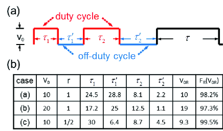
Figure 2: (Color online) (a) Sequence of laser pulses in our experiments. (b) Table of the designed lattice depth $V_{0}$, the parameter $r$ for the target state $|\Psi_{a}\rangle$ in Eq. (7), the durations $\tau_{1,2}$ and $\tau_{1,2}^{\prime}$ given by the numerical maximizing of the fidelity $F$, the fitted value $V_{0R}$ of the lattice depth and the fidelities $F_{R}(V_{0R})$ defined in Eq. (11) for the preparation processes of the cases (a, b, c) in our experiments. Here $V_{0R}$ is given by the fitting of the theoretical values of $N_{0}(\tau)/N$ given by Eq. (9) to the experimental measurements. The units of $V_{0}$ and $V_{0R}$ are $E_{R}$, and the units of $\tau_{1,2}$ and $\tau^{\prime}_{1,2}$ are $\mathrm{{\mu}{s}}$.

Finally we consider the case with $q_{0}\neq 0$, i.e., the target state $|\Psi_{a}\rangle$ is the superposition of the Bloch states with non-zero quasi-momentum. With our approach, we cannot prepare the atoms into such a state in the lab reference. Nevertheless, as shown above, with the laser pulses of optical lattices moving with velocity $-q_{0}/m$, the atoms can be loaded into the state $|\Psi_{a}\rangle$ in the reference moving with these pulses.

III Experimental results

In our experiment, we first prepare a cigar shaped BEC of about $N=1\times 10^{5}$ ⁸⁷Rb atoms in the $|F=2,m_{F}=2\rangle$ hyperfine ground state in the Quadripole-Ioffe configuration trap, of which the axial frequency is $20\mathrm{Hz}$ and the radial frequency $220\mathrm{Hz}$ Liu ; Zhou10 . The 1D optical lattice along the BEC’s long axis ($x$-direction) can be created by laser beams with wavelength $\lambda=2a=852\mathrm{nm}$, which is far beyond the ⁸⁷Rb transition line between $|F=2\rangle$ to $|F^{\prime}=3\rangle$ .

In our experiments we prepare the atoms in the excited-band states of a 1D optical lattice with depth $V_{0}$. We choose the target state to be

$$|\Psi_{a}(V_{0})\rangle=\sqrt{1-r}|s,0;V_{0}\rangle+\sqrt{r}|d,0;V_{0}\rangle,$$ (7)

where $r$ is a real number and $|n,q;V_{0}\rangle$ is the Bloch state in the $n$ band with quasi-momentum $q$. We perform the preparation processes for the cases (a) $V_{0}=10E_{R},r=1$, (b) $V_{0}=20E_{R},r=1$ and (c) $V_{0}=10E_{R},r=1/2$, with $E_{R}=4\pi^{2}\hslash^{2}/(m\lambda^{2})$. As shown in above section, the preparation of the atoms into the state $|\Psi_{a}(V_{0})\rangle$ can be accomplished via switching on and off the standing-wave laser beam for the optical lattice. In our experiment we choose $N_{C}=2$. Namely, the preparation process is accomplished via two duty cycles and two off-duty cycles, as shown in Fig. 2(a). The laser pulses in the duty cycles are generated via a fast response radio frequency switch together with a normal frequency source. As shown in Sec. II, we determine the durations $\tau_{1,2}$ and $\tau_{1,2}^{\prime}$ for the duty and off-duty cycles by numerically maximizing the fidelity $F$ defined in Eq. (6). In Fig. 2(b) we show the values of $\tau_{1,2}$ and $\tau_{1,2}^{\prime}$ and the maximized fidelities given by our numerical calculations. With the same calculation we also obtain the finial state

$$|\Psi_{L}(V_{0})\rangle = \left(e^{-i\frac{p_{x}^{2}}{2m}\tau_{2}^{\prime}}e^{-i[\frac{p_{x}^{2}}{2m}+V_{0}\cos^{2}\left(\frac{\pi x}{a}\right)]\tau_{2}}\times\right.$$ (8)

$$\left.e^{-i\frac{p_{x}^{2}}{2m}\tau_{1}^{\prime}}e^{-i[\frac{p_{x}^{2}}{2m}+V_{0}\cos^{2}\left(\frac{\pi x}{a}\right)]\tau_{1}}\right)|p_{x}=0\rangle$$

$$\equiv \sum_{n}f_{L,n}\left(V_{0}\right)|n,0\rangle$$

of the atoms after the preparation process in cases (a, b, c).

As shown in Sec. II, in the end of the preparation process we instantaneously switch on the optical lattice, and hold it for time $\tau$. Then we switch off the laser beams and the magnetic trap, and image the expanding cloud after $30$ms time of flight using resonant probe light propagating along the $z$-axis. With this approach we can measure the number $N_{j}(\tau)$ of the atoms in the zero-momentum state $|p_{x}=2j\pi/a\rangle$, while the population of the higher momentum states are negligible (less than $5\%$). As shown above, after the preparation process in cases (a, b, c), the atoms prepared in the state $|\Psi_{L}\left(V_{0}\right)\rangle$ in Eq. (8). Thus, when the laser beams and the magnetic trap are switched off, the atomic state is $|\Psi_{\tau}\left(V_{0}\right)\rangle=\sum_{n}f_{L,n}\left(V_{0}\right)e^{-i\mathcal{E}_{n,0}\tau}|n,0\rangle$. Here $\mathcal{E}_{n,0}$ is the eigen-energy of $H_{x}$ with respect to the state $|n,0\rangle$, respectively. Namely, we have $H_{x}|n,0\rangle=\mathcal{E}_{n,0}|n,0\rangle$. Therefore, the number $N_{j}(\tau)$ of atoms in the state $|p_{x}=2j\pi/a\rangle$ at time $\tau$ would be $N_{j}(\tau)=N|\langle p_{x}=2j\pi/a|\Psi_{\tau}\left(V_{0}\right)\rangle|^{2}$, and satisfies

$$\frac{N_{j}(\tau)}{N}=P_{j}(\tau)$$ (9)

with the function $P_{j}(\tau)$ defined as

$$P_{j}(\tau)\equiv\left|\sum_{n}f_{L,n}\left(V_{0}\right)C_{n,j}e^{-i\mathcal{E}_{n,0}\tau}\right|^{2},$$ (10)

with $C_{n,j}$ defined in the above subsection. Eqs. (9) and (10) show that the atom number $N_{j}(\tau)$ oscillates with $\tau$.

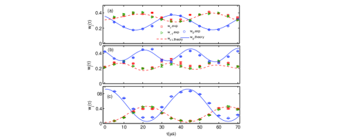
Figure 3: (Color online) The relative population $N_{j}(\tau)/N$ ($j=0,\pm 1$, it is denoted as $\mathrm{w}_{j}(\tau)$ in the figure) for the states with $p_{x}=2j\pi/a$. Here $N_{j}(\tau)/N$ is plotted as a function of the holding time $\tau$ for the cases (a) $V_{0}=10E_{R},r=1$, (b) $V_{0}=20E_{R},r=1$ and (c) $V_{0}=10E_{R},r=1/2$. We show the values of $N_{0}(\tau)/N$ (blue circles with error bar), $N_{1}(\tau)/N$ (red squares with error bar) and $N_{-1}(\tau)/N$ (green triangles with error bar) measured in our experiments and the ones given by our numerical calculation with Eq. (9) and the state $|\Psi_{\tau}(V_{0R})\rangle$ (blue solid line for $N_{0}(\tau)/N$ and red dashed line for $N_{\pm 1}(\tau)/N$), with $V_{0R}$ given by the fitting of the theoretical values of $N_{0}(\tau)/N$ given by Eq. (9) to the experimental measurements.

In Fig. 3 we illustrate the values of $N_{j}(\tau)/N$ ($j=0,\pm 1$) of the state with $p_{x}=\pm 2j\pi/a$ given by our experimental measurements. We also fit the theoretical values of $N_{0}(\tau)/N$ given by Eq. (9) to the experimental results. In our experiments, the values of $\tau_{1,2}$, $\tau_{1,2}^{\prime}$ and $a$ are controlled well. On the other hand, the relative accuracy of the control of $V_{0}$ is more than $90\%$. A relative error of $V_{0}$, which is in the order of one percent, may appear in our preparation process for each case. Due to this fact, in our calculations we use the experimental values of $\tau_{1,2}$, $\tau_{1,2}^{\prime}$ and $a$, and take $V_{0}$ as a fitting parameter. In Fig. 3 we show the values of $N_{j}(\tau)/N$ given by our theoretical calculation with Eq. (9) and the lattice depth $V_{0R}$ given by the fitting calculation. It is shown that the theoretical curve fits well with the experimental results. Therefore, in our experiments the atoms are successfully loaded in the state $|\Psi_{L}\left(V_{0R}\right)\rangle$. It is pointed out that, the theoretical curves of $N_{1}(\tau)/N$ and $N_{-1}(\tau)/N$ are the same, while the experimental data differ by an amount of $5\%$. That difference may be caused by the imperfect alignment of the optical lattice along the long axis of the BEC.

In Fig. 2(b) we display the designed values $V_{0}$ and the realistic values $V_{0R}$ of the lattice depth in our experiments for the cases (a, b, c), and the realistic fidelities

$$F_{R}(V_{0R})=|\langle\Psi_{L}(V_{0R})|\Psi_{a}(V_{0R})\rangle|^{2}$$ (11)

of the preparation processes in our experiments. It is shown that in cases (a) and (b) where the target states are selected to be the single $d$-band Bloch state $|d,0;V_{0}\rangle$, the fidelities $F_{R}(V_{0R})$ of our experimental preparation processes are as high as $98.2\%$ and $97.3\%$. In case (c) where the target state is the superposition state $(|s,0;V_{0}\rangle+|d,0;V_{0}\rangle)/\sqrt{2}$, the fidelity is $99.5\%$. According to these results, in all of our experiments with various target states and lattice depths, the preparation processes are successfully accomplished within several ten micro-seconds via our approach.

IV Collisional decay and lifetime of BEC in excited band

In above sections, we show our approach to load the BEC to the excited band of an optical lattice. As an application, we study decay process of the ⁸⁷Rb BEC loaded in the $d$-band state with zero quasi-momentum of the 1D optical lattice. It is well-known that, the atoms in the excited bands of an optical lattice can decay to the lower bands via inter-atomic collision, and the lifetime of these atoms is usually determined by this collisional decay.

In this section, we first give an analytical calculation for the collisional-decay of the ⁸⁷Rb BEC in our experiments. Then we compare our theoretical result to our experimental measurements. The quantitative agreement between them confirms our analytical result for the collisional decay rate. Our result can be straightforwardly generalized to other systems of weakly interacting BEC in the high energy bands of an optical lattice.

We consider the ultracold bosonic atoms condensed in the $d$-band state with zero quasi-momentum. When two atoms in the condensate decays to lower bands via collision, they likely become thermal due to the large inter-band energy gap. In the beginning of the collisional decay, these collisional products are very rare. Thus, we can neglect the scattering between the thermal atoms and the condensed ones, and only consider the collision of the atoms in the condensate. Therefore, the decreasing of the density $n_{d}(t)$ of the ultracold bosonic atoms condensed in the $d$ band can be described by the master equation ps

$$\frac{dn_{d}\left(t\right)}{dt}=-Kn_{d}\left(t\right)^{2}\,.$$ (12)

Here the factor $K$ is given by

$$K=2\sum_{\left(n_{1},n_{2}\right)\neq(d,d)}\sigma\left(n_{1},n_{2}\right)v,$$ (13)

where $\sigma\left(n_{1},n_{2}\right)$ is the cross-section of the two-atom inelastic collision, with the $i$th ($i=1,2$) atom in the $n_{i}$ band after the collision, and $v$ is the relative velocity of the two atoms before collision. In Eq. (13) the factor $2$ comes from the bosonic statistics. Solving Eq. (12), we obtain

$$n_{d}\left(t\right)=\frac{n_{d}\left(0\right)}{1+Kn_{d}\left(0\right)t},$$ (14)

thus, the decay rate of our system can be defined as $\Gamma=Kn_{d}(0)$.

In the Appendix we calculate the cross-section $\sigma\left(n_{1},n_{2}\right)$ for the system in our experiment, and obtain the result ($\hslash=1$)

$$\sigma\left(n_{1},n_{2}\right)v=\frac{4\pi a_{s}^{2}a^{2}}{m}\int dq\left[\theta\left(2\mathcal{E}_{d,0}-\mathcal{E}_{n_{1},q}-\mathcal{E}_{n_{2},-q}\right)\left|\int_{0}^{a}dxu_{n_{1},q}^{\ast}\left(x\right)u_{n_{2},-q}^{\ast}\left(x\right)u_{d,0}^{2}\left(x\right)\right|^{2}\right],$$ (15)

with $m$ the mass of a single ⁸⁷Rb atom and $a_{s}$ the scattering length of two ⁸⁷Rb atoms. Here $a$ is the lattice constant of the optical lattice, the periodic Bloch function $u_{n,q}(x)$ and the eigen-energy $\mathcal{E}_{n,0}$ of the Hamiltonian $H_{x}$ in the $x$-direction are defined in Sec. II. and Sec. III, respectively. In Eq. (15) the $\theta$-function is defined as $\theta(x)=1$ for $x>0$ and $\theta(x)=0$ for $x<0$.

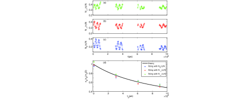
Figure 4: (Color online) (a-c) The fraction $N_{j}(\tau)/N\ (j=0,\pm 1)$ given by our experimental measurements. Here $N_{j}(\tau)$ is the number of the atoms with $p_{x}\approx 2j\pi/a$, and $N$ is the total atom number in the condensate prepared in our experiment. In our experiments we first perform the preparation process for the case (a) in Sec. III, and hold the optical lattice for time $\tau$. (d) The value of $n_{d}(\tau_{0})/n_{d}(0)$ given by the fitting of Eq. (16) with the experimental measurements of $N_{j}(\tau)/N\ (j=0,\pm 1,$ blue dots, green triangles and red suqares with error bars), and the one given by the theoretical calculation with Eq. (14) (black solid line).

In our experiment, the collisional decay of the BEC in excited-band state is observed via the following approach. We first perform the preparation process for the case (a) in the above section, and prepare the ⁸⁷Rb BEC at the state $|\Psi_{L}(V_{0})\rangle=\sum_{n}f_{L,n}\left(V_{0}\right)|n,0\rangle$. Here the depth $V_{0}$ of the optical lattice is $10E_{R}$ and the coefficients $f_{L,n}(V_{0})$ is given by the numerical calculation in Eq. (8), with $\tau_{1,2}$ and $\tau_{1,2}^{\prime}$ given in Fig. 2(b). We have $|f_{d}|^{2}=98\%$. Then we hold the optical lattice for time $\tau$ and measure the number $N_{j}(\tau)\ (j=0,\pm 1)$ of atoms in the state $|p_{x}=2j\pi/a\rangle$. As shown in Fig. 4(a-c), we do the measurements for the cases with $\tau=\tau_{0}+\tau^{\prime}$ with $\tau_{0}=0,300\mathrm{\mu s},600\mathrm{\mu s},900\mathrm{\mu s}$ and $\tau^{\prime}\in(0,100\mathrm{\mu s})$.

Since $\tau^{\prime}$ is much smaller than the characteristic time of the collisional decay in our system, in time evolution of the BEC in the interval $\tau\in(\tau_{0},\tau_{0}+\tau^{\prime})$, the effect given by the collisional decay can be neglected. Therefore, we have the relation $N_{j}^{d}\left(\tau\right)/N=n_{d}\left(\tau_{0}\right)/n_{d}\left(0\right)P_{j}(\tau)$, with $j=0,\pm 1$ and the function $P_{j}(\tau)$ defined in Eq. (9). Here $N$ is the total number of the atoms in the condensate prepared in our experiment. Namely, when $\tau$ is large, $N$ is the summation of the atom number of the remained condensate and the one of the product of the collisional decay. In the above expression $N_{j}^{d}\left(\tau\right)$ is the number of the atoms with $p_{x}=2j\pi/a$ in the remained condensate at time $\tau$. Nevertheless, in our experiments, when $\tau$ is large the atoms in the remained condensate are mixed with some of the thermal atoms produced by the the collisional decay, which have the similar momentum with the condensed ones. It is thus hard for us to exactly measure $N_{j}^{d}\left(\tau\right)$ for the cases with large $\tau$. Therefore, the number $N_{j}$ given by our measurement is actually the summation of the number of condensed atoms and the thermal atoms with $p_{x}\approx 2j\pi/a$ nj . Since the thermal atoms without quantum coherence do not attend the Rabi oscillation, we have

$$\frac{N_{j}\left(\tau\right)}{N}\approx\frac{n_{d}\left(\tau_{0}\right)}{n_{d}\left(0\right)}P_{j}(\tau)+n^{t}_{j}(\tau_{0}).$$ (16)

with $j=0,\pm 1$ and $n^{t}_{j}(\tau_{0})$ the density of the thermal atoms with $p_{x}\approx 2j\pi/a$. It is pointed out that, because $P_{j}(\tau)$ is an oscillating function of $\tau$, the fraction $N_{j}\left(\tau\right)/N$ also oscillates with the time $\tau$. Physically speaking, that is because the quantum coherence is maintained in the remained condensate. As shown in Fig. 4(a-c), such a behavior is clearly observed in our measurements.

We fit expression (16) of $N_{j}(\tau)/N$ with the experimental measurements in each time interval $\tau_{0}<\tau<\tau_{0}+\tau^{\prime}$, and take $n_{d}(\tau_{0})/n_{d}(0)$ and $n^{t}_{j}(\tau_{0})$ as the fitting parameter. In Fig.4(d) we compare the value of $n_{d}\left(\tau_{0}\right)/n_{d}\left(0\right)$ given by such a fitting, and the one given by Eq. (14) with the factor $K$ calculated from Eq. (15) and $n_{d}\left(0\right)=2.39\times 10^{14}~{}\mathrm{cm}^{-3}$. Here we approximate $n_{d}\left(0\right)$ to be the average atomic density of the condensate in our magnetic trap without optical lattice. The good agreement between the theoretical and experimental results confirms our analysis of the decay mechanisms and the calculations of scattering amplitude. In particular, all of the oscillating amplitudes of the curves $N_{0,\pm 1}(\tau)/N$ given by our measurements quantitatively consist with the condensate fraction $n_{d}(\tau_{0})/n_{d}(0)$ given by our theoretical calculation. This consistent shows that in our experiment the quantum coherence are successfully maintained in the un-decayed condensate, and does not exist in the decay products.

V conclusion

In this paper we present a method for effective preparation of a BEC in excited bands of an optical lattice. With our approach the BEC can be prepared in either a pure Bloch state in the excited band or the superposition of Bloch states in different bands via the sequence of standing-wave laser pulses. We experimentally demonstrate our method by preparing the ⁸⁷Rb BEC into the $d$-band state and the superposition of $s$- and $d$-band states of a 1D optical lattice within a few tens of microseconds. We further measure the collisional decay process of the $d$-band BEC prepared in our experiment, and analytically derive the collisional-decay rate atoms in the excited-band states. The experimental and theoretical results consist well with each other. Our method and result are helpful for the study of orbital optical lattice and simulation of condensed matter physics.

VI ACKNOWLEDGMENTS

We thank Hui Zhai, Hongwei Xiong and Xinxing Liu for useful discussions. This work is supported by National Natural Science Foundation of China under Grants No. 61027016, 61078026, 10934010, 11222430, and 11074305, and NKBRSF of China under Grants No. 2011CB921501 and 2012CB922104.

Appendix A the cross-section of inelastic collision between $d$-band atoms

In this appendix we calculate the cross-section $\sigma\left(n_{1},n_{2}\right)$ of the inelastic collision between the two atoms in the $d$-band state with zero momentum, and prove Eq. (15). In the two-atom scattering problem of our system, the total Hamiltonian is given by ($\hslash=1$)

$$H = -\frac{1}{m}\frac{\partial^{2}}{\partial y^{2}}-\frac{1}{m}\frac{\partial^{2}}{\partial z^{2}}+\sum_{i=1,2}\left[-\frac{1}{2m}\frac{\partial^{2}}{\partial x_{i}^{2}}+V(x_{i})\right]$$ (17)

$$+U\left(\vec{r}\right)$$

$$\equiv H_{0}+U\left(\vec{r}\right),$$

with $\vec{r}=(x,y,z)$ the relative position of the two atoms, and $x_{i}$ $(i=1,2)$ the $x$-coordinate of the $i$th atom in the $x$-direction. Namely, we have $x=x_{1}-x_{2}$. In Eq. (17), $V$ is the potential given by the optical lattice in the $x$-direction, and $U\left(\vec{r}\right)$ is the two-atom interaction potential. In this paper we model the inter-atomic interaction with the Huang-Yang pseudo-potential

$$U\left(\vec{r}\right)=\frac{4\pi a_{s}}{m}\delta\left(\vec{r}\right)\frac{\partial}{\partial r}(r\cdot),$$ (18)

where $a_{s}$ the $s$-wave scattering length.

Here we calculate the cross-section with the approach in Sec. 3-e of Ref. taylor . In Eq. (17), $H_{0}$ is defined as the free-Hamiltonian of the two atoms without interaction. The eigen-state of $H_{0}$ can be written as

$$|\lambda,n_{1},n_{2}\rangle\equiv$$

$$\frac{a}{\left(2\pi\right)^{2}}e^{ik_{y}y}e^{ik_{z}z}e^{iq_{1}x_{1}}e^{iq_{2}x_{2}}u_{n_{1},q_{1}}\left(x_{1}\right)u_{n_{2},q_{2}}\left(x_{2}\right),$$

with $k_{y(z)}$ the two-atom relative momentum in the $y$-($z$-) direction and $a$ the lattice constant of the optical lattice. Here $q_{i}$ and $n_{i}$ $(i=1,2)$ are the quasi-momentum and the quantum number for the energy band of the $i$th atom, respectively. As shown in the maintext, $u_{n,q}(x)$ is the periodic Bloch function of the $n$ band with quasi-momentum $q$. We further define

$$\lambda=(k_{y},k_{z},q_{1},q_{2})$$ (20)

as the set of all the four quantum numbers. It is easy to prove that

$$H_{0}|\lambda,n_{1},n_{2}\rangle = \left(\frac{k_{y}^{2}+k_{z}^{2}}{m}+\mathcal{E}_{n_{1},q_{1}}+\mathcal{E}_{n_{2},q_{2}}\right)|\lambda,n_{1},n_{2}\rangle$$ (21)

$$\equiv E_{\lambda,n_{1},n_{2}}|\lambda,n_{1},n_{2}\rangle,$$

where $\mathcal{E}_{n,q}$ is the single-atom energy associated to the $n$-band state with quasi-momentum $q$, and satisfies

$$\left[-\frac{1}{2m}\frac{\partial^{2}}{\partial x^{2}}+V(x)\right][e^{iqx}u_{n,q}(x)]=\mathcal{E}_{n,q}e^{iqx}u_{n,q}(x).$$ (22)

Now we calculate the cross-section of the collision of two atoms in the $d$-band with zero quasi-momentum. According to the standard scattering theory, the cross-section is defined with respect to a two-dimensional plane. Here we assume the plane is spanned by the vectors $\hat{e}_{a}$ and $\hat{e}_{b}$. They satisfy $\hat{e}_{a}\cdot\hat{e}_{b}=0$, and the $x$-component of $\hat{e}_{a(b)}$ is equal to $a$ (Fig. 5). To define the cross-section, we should consider the incident wave packets

$$|\Psi_{\left(\kappa_{a},\kappa_{b}\right)}\rangle=\int dk_{y}dk_{z}dq_{1}dq_{2}e^{-i\left(\kappa_{a}\hat{e}_{a}+\kappa_{b}\hat{e}_{b}\right)\cdot\vec{K}}\phi\left(\lambda\right)|\lambda,d,d\rangle,$$ (23)

where $\kappa_{a},\kappa_{b}$ are two integers, and $\lambda=\left(k_{y},k_{z},q_{1},q_{2}\right)$ is the set of all the four quantum numbers. Here $\phi\left(\lambda\right)\equiv\phi\left(k_{y},k_{z},q_{1},q_{2}\right)$ is a normalized wave packet which sharply peaks at the point $k_{y}=k_{y0},k_{z}=k_{z0},q_{1}=q_{10},q_{2}=q_{20}$, and the vector $\vec{K}$ is defined as $\vec{K}\equiv[(q_{2}-q_{1})/2,k_{y},k_{z}]$. With these assumptions, it is easy to prove that the average two-atom relative position given by the wave function $|\Psi_{\left(\kappa_{a},\kappa_{b}\right)}\rangle$ is distributed in the two-dimensional plane spanned by $\hat{e}_{a}$ and $\hat{e}_{b}$ (Fig. 5).

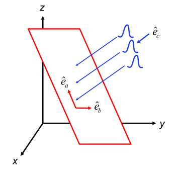
Figure 5: The motion of the wave packets of the two-atom relative coordinate through a two-dimensional plane.

According to the scattering theory, the cross-section $\sigma\left(n_{1},n_{2}\right)$ is defined as

$$\sigma\left(n_{1},n_{2}\right)=\left|\hat{e}_{a}||\hat{e}_{b}\right|\times$$

$$\sum_{\kappa_{a},\kappa_{b}}\int dk_{y}^{\prime}dk_{z}^{\prime}dq_{1}^{\prime}dq_{2}^{\prime}\left|\langle\lambda^{\prime},n_{1},n_{2}|(S-1)|\Psi_{\left(\kappa_{a},\kappa_{b}\right)}\rangle\right|^{2},$$

(24)

where $\lambda^{\prime}=(k_{y}^{\prime},k_{z}^{\prime},q_{1}^{\prime},q_{2}^{\prime})$ and $S$ is the S-operator with respect to the scattering process, and satisfies

$$\langle\lambda^{\prime},n_{1},n_{2}|S|\lambda,d,d\rangle=\langle\lambda^{\prime},n_{1},n_{2}|\lambda,d,d\rangle$$

$$-2\pi i\delta\left(E_{\lambda,d,d}-E_{\lambda^{\prime},n_{1},n_{2}}\right)\langle\lambda^{\prime},n_{1},n_{2}|T|\lambda,d,d\rangle,$$

(25)

with $T$ the associated T-operator.

Therefore, to obtain the scattering cross-section $\sigma\left(n_{1},n_{2}\right)$, we should first calculate the T-matrix element $\langle\lambda^{\prime},n_{1},n_{2}|T|\lambda,d,d\rangle$. In our experiments, since the scattering length of ⁸⁷Rb atoms is much smaller than the atomic de Broglie wavelength and the lattice constant $a$ of the optical lattice, we can use the Born approximation

$$T\approx U\left(\vec{r}\right).$$ (26)

Using the Huang-Yang pseduo-potential in Eq. (18), we obtain

$$\langle\lambda^{\prime},n_{1},n_{2}|T|\lambda,d,d\rangle=\frac{a^{2}a_{s}}{4m\pi^{2}}A$$ (27)

with the parameter $A$ defined as

$$A \equiv \int dx_{1}dx_{2}u_{n_{1},q_{1}^{\prime}}^{\ast}\left(x_{1}\right)u_{n_{2},q_{2}^{\prime}}^{\ast}\left(x_{2}\right)\times$$ (28)

$$\delta\left(x_{1}-x_{2}\right)u_{d,q_{1}}\left(x_{1}\right)u_{d,q_{2}}\left(x_{2}\right).$$

To obtain the value of $A$, we first assume the length of the optical lattice in the $x$-direction is $N_{x}a$. Then the direct calculation gives

$$A=N_{x}\Gamma\left(q_{1},q_{2},q_{1}^{\prime},q_{2}^{\prime}\right)\delta_{q_{1}+q_{2},q_{1}^{\prime}+q_{2}^{\prime}},$$ (29)

where the function $\Gamma\left(q_{1},q_{2},q_{1}^{\prime},q_{2}^{\prime}\right)$ is defined as

$$\Gamma\left(q_{1},q_{2},q_{1}^{\prime},q_{2}^{\prime}\right)$$

$$= \int_{0}^{a}dxu_{n_{1},q_{1}^{\prime}}^{\ast}\left(x\right)u_{n_{2},q_{2}^{\prime}}^{\ast}\left(x\right)u_{d,q_{1}}\left(x\right)u_{d,q_{2}}\left(x\right).$$

Here the Kronecker symbol is defined as $\delta_{ij}=1$ for $i=j$ and $\delta_{ij}=0$ for $i\neq j$. Therefore, for a slow-varying function $f(q_{1},q_{2})$, we have

$$\left(\frac{2\pi}{N_{x}a}\right)^{2}\sum_{q_{1},q_{2}}Af(q_{1},q_{2})$$ (31)

$$= \frac{1}{N_{x}}\left(\frac{2\pi}{a}\right)^{2}\sum_{q_{1}}\Gamma\left(q_{1},q_{1}^{\prime}+q_{2}^{\prime}-q_{1},q_{1}^{\prime},q_{2}^{\prime}\right)f(q_{1},q_{1}^{\prime}+q_{2}^{\prime}-q_{1})$$

$$= \frac{2\pi}{a}\int dq_{1}\Gamma\left(q_{1},q_{1}^{\prime}+q_{2}^{\prime}-q_{1},q_{1}^{\prime},q_{2}^{\prime}\right)f(q_{1},q_{1}^{\prime}+q_{2}^{\prime}-q_{1})$$

$$= \frac{2\pi}{a}\int dq_{1}dq_{2}\Gamma\left(q_{1},q_{2},q_{1}^{\prime},q_{2}^{\prime}\right)f(q_{1},q_{2})\times$$

$$\delta\left[\left(q_{1}^{\prime}+q_{2}^{\prime}\right)-\left(q_{1}+q_{2}\right)\right].$$

Here we have used the relation

$$\left(\frac{2\pi}{N_{x}a}\right)\sum_{q_{1}}=\int dq_{1}$$ (32)

which is applicable in the limit $N_{x}\rightarrow\infty$. The result in Eq. (31) implies

$$A=\frac{2\pi}{a}\Gamma\left(q_{1},q_{2},q_{1}^{\prime},q_{2}^{\prime}\right)\delta\left[\left(q_{1}^{\prime}+q_{2}^{\prime}\right)-\left(q_{1}+q_{2}\right)\right].$$ (33)

Substituting Eq. (33) into Eq. (27), we finally obtain the element of T-matrix

$$\langle\lambda^{\prime},n_{1},n_{2}|T|\lambda,d,d\rangle$$

$$= \frac{aa_{s}}{2m\pi^{2}}\Gamma\left(q_{1},q_{2},q_{1}^{\prime},q_{2}^{\prime}\right)\delta\left[\left(q_{1}^{\prime}+q_{2}^{\prime}\right)-\left(q_{1}+q_{2}\right)\right].$$

(34)

Substituting Eq. (34) into Eqs. (25, 23) and Eq. (24), we can obtain the scattering cross-section $\sigma\left(n_{1},n_{2}\right)$. The straightforward calculation gives

$$\sigma\left(n_{1},n_{2}\right)=\frac{4\pi a_{s}^{2}a^{2}}{m}\int dqdk_{y}dk_{z}dq_{1}dq_{2}\frac{\left|\phi\left(\lambda\right)\right|^{2}}{\left|\partial E_{\lambda,d,d}/\partial k_{\parallel}\right|}$$

$$\times\theta\left(\mathcal{E}_{d,q_{1}}+\mathcal{E}_{d,q_{2}}-\mathcal{E}_{n_{1},\left(q_{1}+q_{2}\right)/2+q}-\mathcal{E}_{n_{2},\left(q_{1}+q_{2}\right)/2-q}\right)$$

$$\times\left|\Gamma\left(q_{1},q_{2},\left(q_{1}+q_{2}\right)/2+q,\left(q_{1}+q_{2}\right)/2-q\right)\right|^{2},$$

(35)

where $k_{\parallel}$ is defined as $k_{\parallel}=(q_{2}-q_{1},k_{y},k_{z})\cdot\hat{e}_{c}$. Here $\hat{e}_{c}$ is the unit vector perpendicular to the plane spanned by $\hat{e}_{a}$ and $\hat{e}_{b}$, i.e., we have $|\hat{e}_{c}|=1$ and $\hat{e}_{c}\cdot\hat{e}_{a}=\hat{e}_{c}\cdot\hat{e}_{b}=0$. In Eq. (35) the derivative $\partial E_{\lambda_{0},d,d}/\partial k_{\parallel}$ is taken for fixed values of $q_{20}+q_{10}$ and $(q_{2}-q_{1},k_{y},k_{z})\cdot\hat{e}_{a}$ and $(q_{2}-q_{1},k_{y},k_{z})\cdot\hat{e}_{b}$. To obtain Eq. (35), we have used the relation

$$\sum_{\kappa_{a},\kappa_{b}}e^{-i\left(\kappa_{a}\hat{e}_{a}+\kappa_{b}\hat{e}_{b}\right)\cdot\vec{J}}=\frac{4\pi^{2}}{\left|\hat{e}_{a}||\hat{e}_{b}\right|}\delta\left(\vec{J}\cdot\frac{\hat{e}_{a}}{\left|\hat{e}_{a}\right|}\right)\delta\left(\vec{J}\cdot\frac{\hat{e}_{b}}{\left|\hat{e}_{b}\right|}\right),$$

with $\vec{J}$ a vector in the three-dimensional space. Moreover, using the fact that $|\phi\left(\lambda\right)|$ is sharply peaked at $\lambda=\lambda_{0}$ and the relations

$$\int dk_{y}dk_{z}dq_{1}dq_{2}\left|\phi\left(\lambda\right)\right|^{2}=1,$$ (37)

$$q_{10}\approx 0,q_{20}\approx 0,k_{y0}\approx 0,k_{z0}\approx 0,$$ (38)

we can further simplify Eq. (35) and obtain the finial expression for the cross-section of inelastic collisions between two $d$-band atoms with zero quasi-momentum:

$$\sigma\left(n_{1},n_{2}\right)=\frac{4\pi a_{s}^{2}a^{2}}{m\left|\left.\partial E_{\lambda,d,d}/\partial k_{\parallel}\right|_{\lambda=\lambda_{0}}\right|}\times$$

$$\int dq\left[\theta\left(2\mathcal{E}_{d,0}-\mathcal{E}_{n_{1},q}-\mathcal{E}_{n_{2},-q}\right)\left|\Gamma\left(0,0,q,-q\right)\right|^{2}\right].$$

(39)

Now we prove Eq. (15). To this end, we need to calculate the component $v$ of the two-atom relative velocity along the direction which is perpendicular to the plane spanned by $\hat{e}_{a}$ and $\hat{e}_{b}$. It is apparent that $v$ is defined as

$$v=\left|\langle\Psi_{\left(\kappa_{a},\kappa_{b}\right)}|-i\frac{\vec{\nabla}_{r}}{m}|\Psi_{\left(\kappa_{a},\kappa_{b}\right)}\rangle\cdot\hat{e}_{c}\right|,$$ (40)

where $\vec{\nabla}_{r}=(\partial/\partial x,\partial/\partial y,\partial/\partial z)$, and the derivative is taken for fixed values of $x_{1}+x_{2}$. With the expression (23) of $|\Psi_{\left(\kappa_{a},\kappa_{b}\right)}\rangle$, it is easy to see that $v$ is independent on the values of $\kappa_{a}$ and $\kappa_{b}$. To calculate the value of $v$, we need the expressions of the periodic Bloch function $u_{d,q}\left(x\right)$ and the single-atom energy $\mathcal{E}_{n,q}$. We find that Eq. (22) for $u_{d,q}\left(x\right)$ and $\mathcal{E}_{n,q}$ can be simplified to

$$\left[-\frac{1}{2m}\frac{\partial^{2}}{\partial x^{2}}+V(x)+h_{1}\right]u_{n,q}(x)=\mathcal{E}_{n,q}u_{n,q}(x)$$ (41)

with $h_{1}=-i(q/m)\left(\partial/\partial x\right)$. Since the $|\phi\left(\lambda\right)|$ is sharply peaked at $(q_{1},q_{2})=(q_{10},q_{20})\approx(0,0)$, we can treat the term $h_{1}$ in the above equation as a perturbation. The second-order perturbation calculation gives the result

$$v=\left|\left.\partial E_{\lambda,d,d}/\partial k_{\parallel}\right|_{\lambda=\lambda_{0}}\right|.$$ (42)

Using Eq. (39) and Eq. (42), we immediately obtain the result in Eq. (15).

References

- (1) O. Morsch, M. Oberthaler, Rev. Mod. Phys. 78, 179 (2006).
- (2) I. Bloch, J. Dalibard, and W. Zwerger, Rev. Mod. Phys. 83, 331 (2011).
- (3) A. Derevianko and H. Katori, Rev. Mod. Phys. 80, 885 (2008).
- (4) V.W. Scarola and S. Das Sarma, Phys. Rev. Lett. 95, 033003 (2005).
- (5) C. Wu et al., Phys. Rev. Lett. 97, 190406 (2006).
- (6) M. Lewenstein and W. V. liu, Nat. Phys. 7, 101(2011).
- (7) M. Ölschläger, G. Wirth, and A. Hemmerich, Phys. Rev. Lett. 106, 015302 (2011).
- (8) T. Müller, S. Fölling, A. Widera, and I. Bloch, Phys. Rev. Lett. 99, 200405 (2007).
- (9) A. Browaeys, H. Häffner, C. McKenzie, S. L. Rolston, K. Helmerson, and W. D. Phillips, Phys. Rev. A 72, 053605(2005).
- (10) G. Wirth, Molschlager, and A. Hemmerich, Nature Phys. 7, 147(2011).
- (11) X. Liu, X. J. Zhou, W. Xiong, T. Vogt, X. Z. Chen, Phys. Rev. A 83, 063402 (2011).
- (12) W. Xiong, X. Yue, Z. Wang, X. J. Zhou, X. Z. Chen, Phys. Rev. A 84, 043616(2011).
- (13) N. Katz, E. Rowen, R. Ozeri, and N. Davidson, Phys. Rev. Lett. 95, 220403 (2005).
- (14) X. J. Zhou, F. Yang, X. G., T. Vogt, and X. Z. Chen, Phys. Rev. A 81, 013615 (2010).
- (15) C. J. Pethick and H. Smith, Bose-Einstein Condensation in Dilute Gases, Cambridge University Press, New York, 2002.
- (16) For the cases with small , e.g., the cases in Sec. III, we also have because in these cases the decay effect is negligible.
- (17) J. R. Taylor, Scattering Theory, Wiley, New York, 1972.