Sounding stellar cycles with Kepler – II. Ground-based observations

Abstract

We have monitored 20 Sun-like stars in the $Kepler$ field-of-view for excess flux with the FIES spectrograph on the Nordic Optical Telescope since the launch of $Kepler$ spacecraft in 2009. These 20 stars were selected based on their asteroseismic properties to sample the parameter space (effective temperature, surface gravity, activity level etc.) around the Sun. Though the ultimate goal is to improve stellar dynamo models, we focus the present paper on the combination of space-based and ground-based observations can be used to test the age-rotation-activity relations.

In this paper we describe the considerations behind the selection of these 20 Sun-like stars and present an initial asteroseismic analysis, which includes stellar age estimates. We also describe the observations from the Nordic Optical Telescope and present mean values of measured excess fluxes. These measurements are combined with estimates of the rotation periods obtained from a simple analysis of the modulation in photometric observations from $Kepler$ caused by starspots, and asteroseismic determinations of stellar ages, to test relations between between age, rotation and activity.

1 Introduction

Some of the greatest advances in our understanding of the solar dynamo during the last few decades have been brought about with the aid of helioseismology. In particular, the mapping of differential rotation inside the Sun (Schou et al., 1998) and constraints on meridional circulation (Hathaway et al., 1996) have helped push forward this understanding. Unfortunately, our inability to make reliable predictions of the evolution of the solar cycle in the transition between solar cycles 23 and 24 implies that solar dynamo models have still not reached a stage where they can be used for predicting the solar cycle.

Observations of activity cycles in Sun-like stars present an excellent opportunity to improve our understanding of the solar dynamo (see e.g. Schrijver & Zwaan, 2008). Asteroseismic observations of activity cycles in Sun-like stars can facilitate this understanding because they allow us to compare the changes taking place in the interior of the stars to the changes taking place on the surface, as discussed by Karoff et al. (2009, hereafter CK09).

Most of the known activity cycles in Sun-like stars were detected first from Mount Wilson Observatory (Wilson, 1978; Baliunas & Vaughan, 1985; Baliunas et al., 1995) and later from Lowell Observatory (Hall et al., 2007). These detections have revealed that around half of the observed Sun-like stars show clear periodic cycles, with periods between 2.5 and 25 years (Baliunas et al., 1995). Brandenburg et al. (1998) and Saar & Brandenburg (1999) showed how 25 stars with well-defined periods can be separated into two groups: a group of young active stars, and a group of older inactive stars. The stars in the former group have cycle periods that are typically 300 times longer than their rotation periods, while the stars in the latter group have cycle periods that are typically only 100 times longer. Durney et al. (1981) (see also Böhm-Vitense (2007); Hall (2008)) suggested that this bifurcation, which is known as the Vaughan-Preston gap (Vaughan & Preston, 1980), is a consequence of the dynamo being seated at two different places inside young and old stars.

The essential hypothesis of Durney et al. (1981) and Böhm-Vitense (2007) is that Sun-like stars will arrive at the main sequence with a nearly homogenous distribution of interior angular momentum. This means that the largest change in the radial rotation rate – the strongest radial shear layer – is found just below the surface of these stars. As the stars evolve they lose angular momentum to stellar winds and if it is assumed that the loss of angular momentum from the surface of these stars only affects the outer convection zone, it follows that a strong shear layer will develop near the bottom of the convection zone – creating a so-called tachocline. This is of course a simplified description of the evolution of angular momentum in Sun-like stars. A more detailed description which includes core-envelope decoupling and disk interactions can be found in e.g. Barnes (2001, 2003, 2007, 2010).

The evolution of stellar angular momentum also has implications for stellar activity levels, as first suggested by Skumanich (1972). These relations imply that stars not only lose angular momentum to stellar winds as they grow older, but they also become less active as they spin down. Skumanich (1972) based his suggestion on observations of the Sun and of three stellar clusters (the Pleiades, Ursa Major and the Hyades) for which ages could be estimated at the time. Since then large efforts have been invested in improving these relations by measuring rotation periods in stellar clusters with known ages (e.g. van Leeuwen & Alphenaar, 1982; Stauffer et al., 1985; Soderblom & Mayor, 1993; Allain et al., 1996; Barnes et al., 1999; Soderblom et al., 2001; Terndrup et al., 2002; Hartman et al., 2009; Meibom et al., 2011a, b).

Asteroseismology offers a unique tool to address this problem because it allows us to measure reliable ages of field stars, independent of rotation period and activity level. If we can also measure the rotation period and activity levels of these stars, they can be used to test and improve the age-rotation-activity relations. In this study, we present age-rotation-activity relations for 10 Sun-like stars with ages between one and 11 Gyr based on asteroseismic measurements.

The shortest activity cycle period measured from the programmes at the Mount Wilson and Lowell observatories is 2.52 years, but three recent results have revealed that Sun-like stars can have even shorter ($<$ 2 years) cycle periods as well. García et al. (2010) detected the signature of a short magnetic activity cycle (period between 120 days and 1 year) in the F5V star HD 49933 using asteroseismic measurements from the CoRoT satellite (Appourchaux et al., 2008). Metcalfe et al. (2010) discovered a 1.6 year magnetic activity cycle in the F8V exoplanet host star $\iota$ Horologii using synoptic Ca HK measurements obtained with the Small and Moderate Aperture Research Telescope System 1.5 m telescope at Cerro Tololo Interamerican Observatory and concluded that if short magnetic activity cycles are common, NASA’s Kepler mission should detect them in the asteroseismic measurements of many additional stars. It is also worth noting that Fletcher et al. (2010) found evidence of a quasi-biennial solar cycle in the residuals of oscillation frequency shifts measured by the Birmingham Solar-Oscillations Network (BiSON, Elsworth et al., 1995) and by the Global Oscillations at Low Frequencies (GOLF, Gabriel et al., 1995) instrument on board the ESA/NASA Solar and Heliospheric Observatory (SOHO) spacecraft. They speculated that this quasi-biennial cycle might be driven by the near surface shear layer – in contrast to the 11-year cycle which is believed to be driven by the tachocline.

These examples of stars with short ($<$ 2 years) cycle periods show that stars can have short cycles, but two stars is too few to reliably judge whether or not short cycle periods are common in Sun-like stars. On the other hand, the results on HD 49933 and $\iota$ Horologii do indicate that dynamos may be fundamentally different in F stars compared to the Sun and other G and K main-sequence stars, most likely due to the thin outer convection zones in F stars. It should be noted here that F-type stars are under-represented in both the Mount Wilson and Lowell samples as the focus of these surveys was on Sun-like stars – in fact no stars earlier than F5 were on the original Mount Wilson list (Wilson, 1978) and this might explain why short periodic cycles were not seen by the Mount Wilson and Lowell surveys.

The layout of the rest of the paper is as follows. In Section 2 we describe the programme, including the target selection and the observations that have been conducted so far. An analysis of these observations can be found in Section 3, and results on both the activity distributions and the age-rotation-activity relations are provided in Section 4. Section 5 includes a discussion of these results.

2 programme description

The programme Sounding Stellar Cycles With Kepler combines high-precision photometric observations from Kepler with ground-based spectroscopic observations from the Nordic Optical Telescope (NOT). The number of targets in the programme was based on the need to have enough stars to cover both sides of the Vaughan-Preston gap (Vaughan & Preston, 1980) and to adequately sample the rotation period vs. cycle period diagram by Böhm-Vitense. These requirements were tempered by the need to obtain the necessary observing time at the NOT each summer and the desirability of observing these targets for the entire length of the Kepler mission, which includes both the nominal and the extended missions (CK09). Based on these considerations, we decided that the programme should include 20 targets.

Ideally, the targets should have been selected prior to the launch of $\it Kepler$ so that observations at the NOT could begin at the same time. We initially tried to follow this approach by selecting targets based on their magnitudes and colours in the Kepler Input Catalog (KIC, Brown et al., 2011), but when we received the first observations from Kepler it was clear that the targets selected prior to launch were not ideal – i.e. the stars did not show oscillations. There are likely two reasons for this: firstly, the stellar properties measured with asteroseismology turned out to be different (Verner et al., 2011) from the less precise parameters implied by the KIC, and secondly, our predictions of how activity and other factors affected the asteroseismic signals were not good enough prior to the launch of Kepler (Chaplin et al., 2011a). We therefore selected a new set of targets in 2010 using the first asteroseismic results from Kepler (Chaplin et al., 2011b).

2.1 Target selection

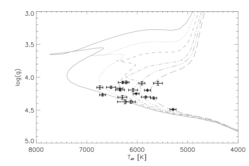
Figure 1: The 20 stars in the programme along with Padova isochrones (Bonatto et al., 2004; Girardi et al., 2002, 2004) calculated for 6 different ages between 1 and 10 Gyr in steps of 0.2 dex, using a metallicity of $Z$ = 0.02.

The 20 stars in the programme are shown in Figs. 1 & 2 along with the same Padova isochrones (Bonatto et al., 2004; Girardi et al., 2002, 2004) that were used in CK09 – the isochrones were calculated for 6 different ages (1.0, 1.6, 2.5, 4.0, 6.3 & 10.0 Gyr), using a metallicity of $Z$ = 0.02. Though the structure and location of the isochrones does depend on the metallicity (Bertelli et al., 2008), it seems safe to conclude that none of the stars have evolved far beyond the main sequence. The names, positions and magnitudes of the 20 stars are given in Table 1 and stellar parameters are found in Table 2.

The basic principles guiding our selection process were:

1. (i) Use stars brighter than 10th magnitude observed in the first 3 months of the Kepler survey phase as candidates.

2. (ii) Preferentially select cooler stars.

3. (iii) Ensure that oscillations can be seen in the acoustic spectrum.

4. (iv) Ensure that the oscillation modes can be understood in the framework of the asymptotic frequency relation.

5. (v) Ensure that hints of rotational splitting can be seen.

6. (vi) Ensure that the small separation is relatively large (6$\mu$Hz).

7. (vii) Ensure that both active and inactive stars have been selected (based on ground-based observations of chromospheric activity in the stars).

The only significant difference between the basic principles given in CK09 and the ones actually used was that, due to the fact that Kepler has been able to do much better photometry on saturated stars than expected (Gilliland et al., 2010), stars as bright as 6.9 were also selected (as can be seen in Table 1). In order to evaluate the small frequency separation and thus the ages of the stars independently from prior investigations, we calculated the autocovariance of each power spectrum (Roxburgh, 2009; Campante et al., 2010; Karoff et al., 2010a).

When we formulated the basic principles for selecting targets, we expected that the stars would be observed for three months in the survey phase of the mission. However, this was changed to only one month (Karoff et al., 2010b). We therefore did not require that rotational splitting could be seen in the spectra calculated from only one month of observations. Instead, we ensured that stars showing rotational modulation from spots in their light curves were selected along with stars that did not show any modulation.

2.2 Asteroseismic results

The calculated autocovariances of the spectra were only used for calculating the small frequency separations and thus to guide the target selection (Roxburgh, 2009; Campante et al., 2010; Karoff et al., 2010a). The stellar properties were inferred with the SEEK package (Quirion et al., 2010). The SEEK package uses a large grid of stellar models computed with the Aarhus STellar Evolution Code (ASTEC; Christensen-Dalsgaard, 2008). To identify the best model, SEEK compares the observational constraints (large and small frequency separations, effective temperature and metallicity) with every model in the grid and makes a Bayesian assessment of the uncertainties. The average large and small frequency separations were obtained as simple mean values of the individual oscillation frequencies from Appourchaux et al. (2012); these frequencies are measured using 9 months of observations – March 22, 2010 to December 22, 2010. The effective temperatures and the metallicities were obtained from Bruntt et al. (2012).

For two stars, we were unable to proceed with the asteroseismic analysis in the standard manner. KIC 10124866 turned out to be an asteroseismic binary with two sets of oscillation frequencies in the acoustic spectrum, which complicates the analysis. A dedicated paper is therefore in preparation by White et al. for this star and no results are thus presented here.

KIC 4914923 was not among the 61 stars analysed by Appourchaux et al. (2012), but it was analysed in the same way as part of more recent work by the same group. The asteroseismic results are presented in Table 2.

2.3 Observations

The photometric asteroseismic observations are described by Appourchaux et al. (2012).

The ground-based observations were obtained with the high-resolution FIbre-fed Echelle Spectrograph (FIES) mounted on the 2.6 meter Nordic Optical Telescope (Frandsen & Lindberg, 2000). Sufficient time was awarded to obtain spectra on three epochs for each star during each year of the nominal $Kepler$ mission in 2010, 2011 and 2012. Observations were obtained using the low-resolution fiber (R=25000). The epochs were typically placed in April, June and August. The spectra were obtained with 7 minute exposures resulting in a S/N above 100 at the blue end of the spectrum for the faintest stars. A few stars are missing observations at one or more epochs – either due to bad weather or passing clouds or due to cosmic ray hits, but most stars have observations at most epochs.

As described above we used effective temperatures and the metallicities from Bruntt et al. (2012) and oscillation frequencies from Appourchaux et al. (2012) in the asteroseismic analysis. For the analysis of the spectra we used $B-V$ measurements of the stars from Høg et al. (2000), which are listed in Table 1, together with Hipparcos luminosities for the Hipparcos stars in the sample.

2.4 Data reduction

The reduction of the spectra, which includes bias and flat-field subtraction, blaze correction, wavelength calibration and removal of cosmic ray hits, was done using FIEStool. FIEStool returns 1-D echelle spectra. We then merged the orders that covers the range between 3885 and 4015 Å and cross-correlate these merged spectra with a solar spectrum to place the observed spectra on a reference wavelength grid with velocities zeroed.

3 Analysis

In order to calculate the excess flux from the stars $\Delta\mathcal{F}_{\rm Ca}$(defined as the surface flux arising from magnetic sources) we have followed Hall et al. (2007) as closely as possible. This recipe contains the following steps (described in more detail below):

1. (i) Correct for blanketing

2. (ii) Normalize the spectra to an absolute flux scale

3. (iii) Measure the flux in a 1Å bandpass $\mathcal{F}_{\textup{1\text{\AA}}}$

4. (iv) Correct for photospheric flux $\mathcal{F}_{\rm phot}$

5. (v) Correct for colour-dependent basal flux $\mathcal{F}_{\rm min}$

6. (vi) Calculate the excess flux $\Delta\mathcal{F}_{\rm Ca}$

The underlying idea here is that the flux in the cores of the Ca H and K lines (which we denote $\mathcal{F}_{\textup{1\text{\AA}}}$) contains the following components (see Schrijver et al., 1989, for discussion of this):

• – Flux from photospheric line wings outside the H₁ and K₁ minima. In contrast to the chromosphere, the photosphere is assumed to be in radiative equilibrium. We denote this component $\mathcal{F}_{\rm phot}$.

• – Basal flux from a optically thick chromosphere that is unrelated to dynamo fields. We denote this component $\mathcal{F}_{\rm min}$.

• – Excess flux. This is the surface flux arising from magnetic sources – i.e. a dynamo. This is the flux which we are interested in measuring. We denote this component $\Delta\mathcal{F}_{\rm Ca}$.

It follows that:

$$\Delta\mathcal{F}_{\rm Ca}=\mathcal{F}_{1\text{\AA}}-\mathcal{F}_{\rm phot}-\mathcal{F}_{\rm min}$$ (1)

3.1 Correcting for blanketing

We first correct the spectra for line blanketing – the decrease in intensity due to many closely spaced and thus unresolved lines. We use the blanketing coefficients from Hall & Lockwood (1995):

$$\epsilon^{\prime}(3912)=1.032-0.296(B-V)$$ (2)

$$\epsilon^{\prime}(4000)=1.060-0.167(B-V)$$ (3)

The correction is applied by making a linear fit through the two spectral points at $\lambda$3912 and $\lambda$4000 and then adjusting the values of this fit to $\epsilon^{\prime}(3912)$ and $\epsilon^{\prime}(4000)$.

3.2 Normalising the spectra to an absolute flux scale

In order to convert the spectra to absolute flux we use the absolute flux scale from Hall et al. (2007):

$${\rm log}\mathcal{F}\left(\Delta\lambda\right)=8.179-2.887(b-y),-0.10\leq b-y\leq 0.41$$ (4)

$${\rm log}\mathcal{F}\left(\Delta\lambda\right)=8.906-4.659(b-y),0.41\leq b-y\leq 0.80$$ (5)

$\mathcal{F}\left(\Delta\lambda\right)$ is calculated as the flux density between $\lambda$3925 and $\lambda$3975 in units of ergs cm^-2 s^-1 Å^-1.

The Strömgren $b-y$ colour indices were calculated using the transformations from Alonso et al. (1996):

$$\theta_{\rm eff}= 0.537+0.854(b-y)+0.196(b-y)^{2}$$

$$- 0.198(b-y)c_{1}-0.026(b-y)\left[{\rm Fe/H}\right]$$

$$- 0.014\left[{\rm Fe/H}\right]-0.009\left[{\rm Fe/H}\right]^{2}$$

where $\theta_{\rm eff}=(5040\,{\rm K})/T_{\rm eff}$ and assuming $c_{1}$=0.35.

3.3 Measuring $\mathcal{F}_{\textup{1\text{\AA}}}$

The next step is to measure the integrated flux in a 1Å bandpass $\mathcal{F}_{\textup{1\text{\AA}}}$ centred on the cores of the K and H lines. This is easily done in the wavelength corrected and velocity-zeroed spectra simply by summing the flux in the 1Å bandpass.

3.4 Correcting for photospheric flux $\mathcal{F}_{\rm phot}$

The 1Å bandpass flux $\mathcal{F}_{\textup{1\text{\AA}}}$ centred on the cores of the K and H lines will contain flux from the photosphere and from a colour-dependent basal flux, which could have an acoustic origin (see, e.g., the review by Schrijver, 1995).

In order to correct for the photospheric flux we need to calculate the separation $W_{0}$ between the two emission lines in the Ca cores (see Hall et al., 2007). This value can be calculated from Lutz & Pagel (1982):

$${\rm log}W_{0}=-0.22{\rm log}g+1.65{\rm log}T_{\rm eff}+0.10[{\rm Fe/H}]-3.39$$ (7)

In Fig. 3 we have plotted $W_{0}$ as a function of effective temperature for the isochrones also used in Fig. 1.

We then calculate the flux from the photosphere by adjusting the integrated flux in the 1Å bandpass ($\mathcal{F}_{\textup{1\text{\AA}}}$) for the ratio between the fluxes in the $W_{0}$ and the 1Å bandpass:

$$\frac{\mathcal{F}(W_{0})}{\mathcal{F}(1\text{\AA})}=W_{0}\mathcal{F}_{1\text{\AA}}^{1/4}$$ (8)

This ratio has also been corrected for the $\mathcal{F}$^1/4 activity scaling law from Ayres (1979), and can be found in Fig. 4. Note that the flux in the $W_{0}$ bandpass is equivalent to the flux between the K₁ minima $\mathcal{F}({\rm K}_{1})$ used by Hall et al. (2007).

3.5 Correcting for colour-dependent basal flux $\mathcal{F}_{\rm min}$

Hall et al. (2007) obtained a relation between the Strömgren $b-y$ colour indices and the photospheric contribution to the measured flux which can be used to correct these for the basal flux. We did try to use this relation along with $b-y$ colour indices calculated using the relations from Alonso et al. (1996), but the resulting values for the basal flux were significantly overestimated resulting in negative values of $\Delta\mathcal{F}_{\rm Ca}$. We therefore adopted our own formulation of the basal flux – estimated from the effective temperatures rather than the $b-y$ colour indices. This was done by making a linear fit to the mean fluxes in Fig. 5 and then lowering the fit values by $3\sigma$ in order to get a representation of the lower level of the mean fluxes as function of effective temperature. The new formulation of the basal flux is:

$${\rm log}\mathcal{F}_{\rm min}=3.07-5.11\cdot 10^{-4}T_{\rm eff}.$$ (9)

Note here that a number of different formulations exist in the literature for the basal flux (see Schrijver, 1995, for discussion of this). The differences in these formulations most likely arise from slightly different instrument configurations and data reduction procedures, which also explains why we need to adopt our own formulation. We did test the effect on the final results of changing the formulation. This was done by varying the values of the lower level of the mean fluxes, which did not lead to any significant changes in the final results.

3.6 Calculating the $S$ index

The most commonly used expression for stellar chromospheric activity is the dimensionless $S$ index obtained from the spectrophotometers used in the Mount Wilson survey. Unfortunately, the $S$ index is sensitive to both the instrument configuration and the spectral resolution (Hall et al., 2007). This is often accounted for by including a normalization constant $\alpha$. This constant is then calculated by observing a large number of stars from the Mount Wilson and Lowell surveys and using these stars as reference stars (see e.g. Wright et al., 2004), but due to the intrinsic variability of the stars this number needs to be relatively large – i.e. larger than our target list.

We therefore adopted another approach and calculated the $S$ index as in Hall et al. (2007) by measuring the flux in the H and K line cores using a 1.09 Å FWHM triangular filter as well as in two 20 Å reference bandpasses centred on $\lambda$3901.067 ($V$) and $\lambda$4001.067 ($R$).

The relationship between the $S$ index and $\mathcal{F}_{\textup{1\text{\AA}}}$ was then used to calibrate the $S$ index. This is done by calculating a pseudo $S$ index called $S^{\prime}$ based on $\mathcal{F}_{\textup{1\text{\AA}}}$:

$$\mathcal{F}_{\textup{1\text{\AA}}}=10^{-14}S^{\prime}C_{\rm cf}T_{\rm eff}^{4},$$ (10)

where $C_{\rm cf}$ is given as (Rutten, 1984):

$${\rm log}\left(C_{\rm cf}\right)=0.45-0.066(B-V)^{3}-0.25(B-V)^{2}-0.49(B-V),$$ (11)

We then obtain a linear relation between the observed $S$ index called $S_{o}$ and the pseudo $S$ index ($S^{\prime}$) which we can use to calibrate the $S$ index. In this way the observed $S$ index ($S_{o}$) is related to the $S$ index according to:

$$S=16.6S_{o}.$$ (12)

The constant of 16.6 is similar to the $\alpha$ calibration constant normally used to account for different spectral coverage and resolution when measuring the $S$ index with different instruments, and it normally lies between 1.8 and 5 (see Gray et al., 2003; Wright et al., 2004; Gray et al., 2006; Hall et al., 2007). The larger value found here is mainly due to the higher resolution of the NOT FIES spectra compared to other instruments that have been used to measure the $S$ index.

3.7 Comparison to HD 157214

The G0V star HD 157214 is at (17:20:39.30 +32:28:21.15) located close to the $Kepler$ field and this star is also part of the priority 1 list of stars being observed with the Solar-Stellar Spectrograph at Lowell Observatory. We have therefore observed this star together with the other stars on most observing nights. With the procedure described above we measure a mean excess flux of $4.8\pm 0.2\cdot 10^{5}{\rm ergs}$ ${\rm cm}^{-2}{\rm s}^{-1}$ and a mean $S$ index of $0.147\pm 0.004$ (where 0.004 is the uncertainty on the mean value). Hall et al. (2007) report a mean $S$ index of 0.162 and an excess flux that varies around $4.5\cdot 10^{5}{\rm ergs}$ ${\rm cm}^{-2}{\rm s}^{-1}$ between 1995 and 2007, but speculate that this star might be heading into an activity minimum. This speculation is supported by observations in 2008 and 2009, where the measured $S$ index of this star was 0.152 (Hall, private communication). Our mean $S$ index of $0.147\pm 0.004$ is therefore in agreement with Hall et al. (2007) – given that the star has been observed at different activity phase and epoch.

The better agreement between the mean values of the excess flux, compared to the $S$ index, measured by Hall et al. (2007) and us could reflect the fact that the external precision is much lower for the $S$ index than for the excess flux. In other words, the given instrument configuration is more important for the $S$ index than for the excess flux. This means that uncertainties in the $\alpha$ constant in eq. 12 lead to larger relative differences (of the order of 10%, Hall et al., 2007) in the $S$ index compared to the excess flux. Also, as the uncertainties we quote are calculated as the uncertainties of the mean values, they reflect only internal uncertainties and do not include offsets or biases between the observations presented here and the observations by e.g. Hall et al. (2007).

3.8 Comparison to Isaacson & Fischer (2010)

The $S$ index has also been measured for three stars in the sample by the California Planet Search program (Isaacson & Fischer, 2010). They obtained one measurement of KIC 6116048 on 22 July 2010, 33 measurements of KIC 8006161 between 26 June 2005 and 4 June 2009 and 27 measurements of KIC 12258514 between 25 April 2010 and 15 September 2010. The mean values and the standard deviations of their and our measurements are provided in Table 3. As can been seen in the table the mean values agree within one standard deviation for KIC 6116048 and KIC 12258514. The $S$ index of KIC 8006161 has also been measured by Duncan et al. (1991) who measured a mean $S$ index of 0.232 with a standard deviation of 0.004 between 2 May 1978 and 17 July 1978. Comparing the three mean values of the $S$ index of KIC 8006161 it appears that it has been declining between 1978 and now – which could explain why we do not have agreement within one standard deviation between the mean value by Isaacson & Fischer (2010) and the mean value by us.

3.9 Rotation Periods

Stellar rotation periods can be measured in the white-light observations from Kepler simply by calculating a periodogram and identifying the highest peak in this periodogram (see e.g. McQuillan et al., 2012; Nielsen & Karoff, 2012; Nielsen et al., 2013). Though this method is simple, care is needed since the method can be susceptible to bias, e.g. the highest peak could be the second or third harmonic of the true rotation period. Part of this problem can be solved by comparing the estimated rotation periods to independent estimates from e.g. $v$sin$i$ measurements and asteroseismology. Results of such a analysis will be presented elsewhere (García et al., in preparation.). Here we present rotation periods for only a limited number of stars for which rotation periods could be unambiguously identified; even these periods may change slightly when additional Kepler observations become available.

We searched for rotational modulations of the light curves by calculating a least-square periodogram (Lomb 1976, see also Karoff 2008). The periodograms were calculated from 14 quarters of $Kepler$ observations that were gathered between 13 May 2009 and 3 October 2012. For this part of the analysis we only used long-cadence observations because not all short-cadence observations were available in a PDC (Pre-search Data Conditioning) processed format. The higher time-resolution of the short-cadence data is only needed for the asteroseismic analysis and not for searching for rotational modulations in the light curves. The PDC processed observations have a significantly reduced number of artifacts that could mimic a spot on the surface of the stars compared to the Simple Aperture Photometry (SAP) generated by the PA (Photometric Analysis) pipeline module.

The periodograms were calculated for 1000 periods between 0 and 20 days in each of the 14 quarters of data for each star. We then identified any peaks in these periodograms with a S/N higher than 4 and crosschecked these peaks with the signal in the light curves. For a star to be assigned a rotation period, the same peak was required to be visible in the periodograms during all 14 quarters and in the light curves.

To validate these rotation periods we compare them in Fig. 6 with the values one would obtain from the $v$sin$i$ measurements by Bruntt et al. (2012; see Table 2) and the asteroseismic radii (Table 2). Indication of a linear trend is seen in the figure, but most of the data points fall above the linear relation indicated by the solid line. This is expected since: 1) sin$i$ will take values between zero and one, 2) it seems natural to expect spots to form close to the fastest rotation latitudes on the stellar surfaces, and 3) there are inherent uncertainties in the $v$sin$i$ measurements – such as choosing the macroturbulence parameter, etc.

Isaacson & Fischer (2010) detected a 19-day rotation period in KIC 12258514, which is consistent with the fact that we do not see any significant peaks in our periodograms calculated between 0 and 20 days. They also detected a 43-day period in KIC 8006161. Originally we did detect a 10-day period in the periodograms of KIC 8006161 calculated as described above. In order to solve this incongruence we calculated new periodograms for 3000 periods between 0 and 60 days. The periodograms revealed that KIC 8006161 shows longer more prominent periods than the 10-day period. None of these periods could meet the criteria described above and no rotation period was thus assigned to KIC 8006161. The same phenomenon was seen in KIC 6116048.

In total we were able to assign a rotation period to 10 out of the 19 stars. Periodograms for these 10 stars are shown in Appendix 1. We note that some of the remaining stars are likely to have rotation periods longer than 20 days.

4 Results

We have measured both the $S$ index and the excess flux $\Delta\mathcal{F}_{\rm Ca}$ for each of our stars (see Table 2). The main difference between these two quantities is that different colour-dependent terms have been removed from the excess flux $\Delta\mathcal{F}_{\rm Ca}$ (Hall et al., 2007). These terms become important when comparing the measured activity level in the stars to stellar properties. Here the excess flux is the best quantity to use because it is corrected for the different colour-dependent terms. Another way to explain the difference between the $S$ index and the excess flux is that the $S$ index is a relative measurement of the activity in the stars – relative in the sense that it measures the intensity in the $H$ and $K$ bandpasses relative to the $R$ and $V$ bandpasses. The excess flux, on the other hand, is an absolute measurement of the activity of the stars – corrected for terms that are not related to (magnetic) activity.

All of the results we present here are mean values of the measured quantities in the 8 different epochs that have been observed so far, and the error bars represent the uncertainties on the mean values. Fig. 7 compares the measured mean $S$ index to the mean excess flux. A clear log-linear relation is seen for all 19 stars except one, which is KIC 8006161. KIC 8006161 has a mean $S$ index of $0.172\pm 0.002$, which is comparable to the mean value seen in the Sun, but the excess flux is only $9.8\pm 1.4\cdot 10^{4}$ ergs cm^-2 s^-1, which is close to the quiet Sun. A handful of stars showing a similar behaviour (not obeying the linear relation between the $S$ index and the excess flux and showing lower than expected excess flux) were identified by Hall et al. (2007) – the most prominent being $\tau$ Cet. $\tau$ Cet has long been suspected of being a Maunder minimum star (Judge et al., 2004) and it will therefore be interesting to see whether KIC 8006161 also shows low variability in the excess flux.

We have also analysed the relationship between the relative variability of the $S$ index and the excess flux and the mean value of these parameters (Figs. 8 & 9). The relation for the excess flux generally follows the same trend that was seen by Hall et al. (2007).

4.1 Activity distributions

Vaughan & Preston (1980) were the first to note an apparent deficit in the number of F-G stars exhibiting intermediate activity. This gap, which is now known as the Vaughan-Preston gap, has been studied extensively since then. One of the largest studies of the gap was performed by Henry et al. (1996), who showed that two Gaussian functions were needed to satisfactorily model the activity distribution of more than 800 southern stars within 50 pc.

To evaluate how the stars in this study are distributed around the Vaughan-Preston gap, we have calculated the distributions for both the $S$ index and the excess flux in Figs. 10 & 11. The bimodal distribution in stellar activity cannot be clearly identified in either of the two histograms. This is in agreement with the results from Hall et al. (2007) who were also unable to find clear indications of a bimodal distribution (Fig. 12 in their paper). In fact our distribution looks almost identical to the distribution of Hall et al. (2007), although it should be borne in mind that they have 143 stars and we have only 19. A Kolmogorov-Smirnov test comparing the two distributions yields a p-value of 0.78, supporting the contention that the measurements arise from the same underlying distributions.

If simple counting statistics were adopted for the uncertainties of each bin, it would, on the other hand, become clear that we would not be able to see a bimodal distribution, even if it were intrinsic here as we only have 19 stars in our sample.

4.2 Age-Rotation-Activity Relations

It was suggested by Skumanich (1972) that there exists a power-law relation between rotation and activity on the one side and age on the other. This study forms the basis for an assumption of a causal relationship between age, rotation and activity – the so-called age-rotation-activity relations (see e.g. Soderblom et al., 2001; Barnes, 2007, or the discussion in the introduction). However, as discussed in the introduction, the number of data points used for calculating these relations leaves room for improvement – especially for stars of solar age or older. The 10 stars for which we have measured rotation periods provide such an improvement.

Despite the lack of Sun-like stars with independently measured ages that can be used to improve the relations by Skumanich (1972), much work has gone into improving the theoretical understanding of these relations (see e.g. Kawaler, 1988; Pinsonneault et al., 1990) and it is clear that no simple log-linear relation between age, rotation and activity exist in general for F-G main sequence stars (see e.g. Noyes et al., 1984; Soderblom et al., 1991; Donahue, 1998; Mamajek & Hillenbrand, 2008). In other words, when more data than the four points used by Skumanich (1972) are available, it is not obvious that all the new data points should follow the simple log-linear relations. Nevertheless, we have fitted all of our measured age-rotation-activity relations with log-linear fits for illustrative purposes.

The first relation we have looked at is the relation between the rotation period and the excess flux in Fig. 12. A log-linear relation is clearly seen in the figure, and is represented by the solid line given by:

$$\log\Delta\mathcal{F}_{\rm Ca}=(-0.74\pm 0.03)\log P_{\rm rot}+6.55\pm 0.02$$ (13)

The exponent of $-0.74\pm 0.03$ is in agreement with the original result by Skumanich (1972).

The second relation is between the age and the excess flux in Fig. 13. The log-linear relation found here is given by:

$$\log\Delta\mathcal{F}_{\rm Ca}=(-0.61\pm 0.17)\log{\rm Age}+6.08\pm 0.13$$ (14)

The important parameter to compare here is the exponent $-0.61\pm 0.17$. Skumanich (1972) found this value to be $-0.54$ and Soderblom et al. (1991) found it to be $-0.66$ (though for $R^{\prime}_{\rm HK}$ instead of $\Delta\mathcal{F}_{\rm Ca}$). Our result does in other words agree with both results within $1\sigma$.

The last relation to analyse is between the rotation period and the age in Fig. 14. Here the log-linear relation is given by:

$$\log P_{\rm rot}=(0.45\pm 0.19)\log{\rm Age}+0.59\pm 0.29$$ (15)

The exponent of $0.45\pm 0.19$ compares nicely to the value of $0.51$ found by Skumanich (1972).

It has been shown by e.g. Barnes (2003) that the rotation period is not only a function of age, but also of colour (or, equivalent, mass). The reason for this is likely that different spin-down time scales exist for stars of different masses. We have therefore included a $B-V$ colour term in the model. This was done in a way similar to that demonstrated by Barnes (2003), although in the function $f$ we have replaced the value 0.50 used by Barnes to 0.38, to account for the range in $B-V$ of the 10 stars in this study (the different offsets does not have any other implications). This provided us with the following relation between rotation, age and $B-V$ colour (see Fig. 15):

$$\log P_{\rm rot}=(0.81\pm 0.10)\log{\rm Age}+\log f(B-V)+0.47\pm 0.22,$$ (16)

where

$$f(B-V)=\sqrt{B-V-0.38}-0.15(B-V-0.38).$$ (17)

The reduced $\chi^{2}$ value of this fit was 1.46, which is lower than the value of 2.57, which we obtain if we use the Skumanich model (eq. 15).

5 Discussion

We have chosen to measure both the excess flux and the $S$ index. This was done as it was the only way to calibrate our measured $S$ indices. Validations of the results presented here have, on the other hand, also shown us that we can obtain a much stronger relation between stellar properties measured with asteroseismology and measured values of the excess flux than with measured values of the $S$ index. This strengthens the general proposition that the $S$ index includes a number of (colour dependent) terms that do not relate to the evolution of stellar angular momentum and activity (Middelkoop, 1982; Rutten, 1984; Rutten & Schrijver, 1987; Hall et al., 2007).

5.1 Do we cover both sides of the Vaughan-Preston gap?

One of the main goals of the target selection was to ensure that the selected targets would cover both sides of the Vaughan-Preston gap. From Fig. 11 it seems that we have only partly succeeded in this – all the stars appear to fall on the inactive branch with $S$ indices less than 0.2. Of course a histogram made from 19 data points must be taken with caution, and some of the 19 stars apparently on the inactive branch might turn out to be active stars. This is also reflected in Fig. 10 where we see that our distribution of 19 stars is in agreement with the distribution of 143 obtained by Hall et al. (2007). This suggests that we are sampling typical excess fluxes for Sun-like stars and that our sample also includes six stars on the active sequence with log$\Delta\mathcal{F}_{\rm Ca}$ above 6 (contradicting what is seen in the results based on the $S$ index). The asteroseismic ages of the stars also suggest that we do cover stars on both sides of the gap.

5.2 What can we learn from the Age-Rotation-Activity Relations?

The 10 stars for which we have independent measurements of asteroseismic ages, rotation periods and excess flux generally all fulfill the Skumanich relations. The possible exception here is the Sun, whose rotation rate and excess flux seem to be significantly lower than predicted by the Skumanich relation, KIC 8006161 (star i in Table 2), whose excess flux also seems to be lower than predicted by the Skumanich relation, and KIC 11244118 (star p in Table 2), whose rotation period seems longer than predicted by the Skumanich relation. A possible explanation for the low excess flux of KIC 8006161 could be that it is in a Maunder minimum state. The long rotation period of KIC 11244118 could be related to the fact that, with an age of 6.3${}_{-4.3}^{+1.2}$ Gyr, it is a relatively old star considering its mass of 1.23${}^{+0.10}_{-0.08}$ M_☉; in other words this star is likely the most evolved star in the sample and might not be a main-sequence star, but a sub-giant (which is also in agreement with its location in Fig. 1).

Barnes (2003) suggested that the relation between stellar rotation period and age separated into two sequences – one for Sun-like stars called the interface sequence and one for the younger G, K and M dwarfs called the convective sequence. As expected we are not able to identify this bifunctionality in the 10 stars analysed here. The reason for this is likely that none of the 10 stars are so young that they fall on the convective sequence.

Table 1: Target list for the sounding stellar cycles with Kepler programme. We also list the Kepler magnitude, $B-V$ values from Høg et al. (2000) and Hipparcos luminosities in units of solar luminosities from The Hipparcos and Tycho Catalogues (ESA 1997) for the the Hipparcos stars in the sample.

KIC ID	$\alpha$ (2000)	$\delta$ (2000)	$k_{p}$	$B-V$	$L$
01435467	19:28:19.84	37:03:35.3	8.9	0.47$\pm$0.02
02837475	19:10:11.62	38:04:55.9	8.4	0.43$\pm$0.02
03733735	19:09:01.92	38:53:59.6	8.4	0.41$\pm$0.02	3.79$\pm$0.49
04914923	19:16:34.88	40:02:50.1	9.4	0.62$\pm$0.03	2.32$\pm$0.58
06116048	19:17:46.34	41:24:36.6	8.4	0.57$\pm$0.01
06603624	19:24:11.18	42:03:09.7	9.0	0.76$\pm$0.03
06933899	19:06:58.34	42:26:08.2	9.6	0.59$\pm$0.04
07206837	19:35:03.72	42:44:16.5	9.7	0.46$\pm$0.06
08006161	18:44:35.14	43:49:59.9	7.3	0.87$\pm$0.01	0.61$\pm$0.02
08379927	19:46:41.28	44:20:54.7	6.9	0.58$\pm$0.01	1.05$\pm$0.08
08694723	19:35:50.58	44:52:49.8	8.8	0.48$\pm$0.02
09098294	19:40:21.20	45:29:20.9	9.7	0.68$\pm$0.08
09139151	18:56:21.26	45:30:53.1	9.1	0.52$\pm$0.03	1.63$\pm$0.40
09139163	18:56:22.12	45:30:25.2	8.3	0.49$\pm$0.01	3.88$\pm$0.69
10124866	18:58:03.46	47:11:29.9	7.9	0.57$\pm$0.02
10454113	18:56:36.62	47:39:23.0	8.6	0.52$\pm$0.02	2.60$\pm$0.36
11244118	19:27:20.48	48:57:12.1	9.7	0.78$\pm$0.05
11253226	19:43:39.62	48:55:44.2	8.4	0.39$\pm$0.02	4.22$\pm$0.61
12009504	19:17:45.80	50:28:48.2	9.3	0.55$\pm$0.03
12258514	19:26:22.06	50:59:14.0	8.0	0.59$\pm$0.01	2.84$\pm$0.25

Table 2: Measured stellar properties. The short names refer to the symbols used in Figs. 2, 8 & 9. The stellar parameters are measured with asteroseismology. $T_{\rm eff}$ and $v$sin$i$ values are from Bruntt et al. (2012). $P_{\rm rot}$, log $<\Delta\mathcal{F}_{Ca}>$ and $<S>$ values are from this study.

KIC	Short	$T_{\rm eff}$ [K]	[Fe/H]	log $g$	$M$[M⊙]	$R$ [R⊙]	age [Gyr]	$v$sin$i$ [km/sec]	$P_{\rm rot}$ [days]	log $<\Delta\mathcal{F}_{\rm Ca}>$	$<S>$
01435467	a	6222$\pm$60	-0.01$\pm$0.06	4.077${}^{+0.020}_{-0.016}$	1.22${}^{+0.10}_{-0.09}$	1.66${}^{+0.04}_{-0.04}$	4.2${}^{+1.2}_{-1.5}$	10.0	7.2 $\pm$ 0.3	5.97 $\pm$ 0.01	0.157 $\pm$ 0.001
02837475	b	6741$\pm$60	-0.02$\pm$0.06	4.155${}^{+0.026}_{-0.026}$	1.36${}^{+0.06}_{-0.10}$	1.60${}^{+0.04}_{-0.04}$	2.0${}^{+0.9}_{-0.8}$	23.5	3.7 $\pm$ 0.1	6.13 $\pm$ 0.01	0.166 $\pm$ 0.001
03733735	c	6687$\pm$60	-0.04$\pm$0.06	4.268${}^{+0.015}_{-0.016}$	1.30${}^{+0.07}_{-0.05}$	1.39${}^{+0.03}_{-0.03}$	1.0${}^{+1.0}_{-0.7}$	16.8	2.6 $\pm$ 0.1	6.22 $\pm$ 0.01	0.182 $\pm$ 0.001
04914923	d	5798$\pm$60	0.17$\pm$0.06	4.198${}^{+0.015}_{-0.016}$	1.11${}^{+0.10}_{-0.08}$	1.39${}^{+0.04}_{-0.04}$	7.6${}^{+2.6}_{-3.1}$	3.6	8.1 $\pm$ 0.4	5.46 $\pm$ 0.12	0.137 $\pm$ 0.005
06116048	e	6022$\pm$60	-0.24$\pm$0.06	4.250${}^{+0.009}_{-0.011}$	0.92${}^{+0.04}_{-0.06}$	1.19${}^{+0.02}_{-0.02}$	8.9${}^{+2.1}_{-1.9}$	4.0	–	5.70 $\pm$ 0.02	0.152 $\pm$ 0.001
06603624	f	5673$\pm$60	0.28$\pm$0.06	4.316${}^{+0.008}_{-0.007}$	1.00${}^{+0.03}_{-0.04}$	1.15${}^{+0.01}_{-0.02}$	11.1${}^{+1.4}_{-1.5}$	3.0	–	5.47 $\pm$ 0.07	0.155 $\pm$ 0.004
06933899	g	5907$\pm$60	0.02$\pm$0.06	4.091${}^{+0.014}_{-0.014}$	1.15${}^{+0.07}_{-0.07}$	1.59${}^{+0.03}_{-0.03}$	4.9${}^{+2.3}_{-1.6}$	3.5	–	5.70 $\pm$ 0.05	0.149 $\pm$ 0.003
07206837	h	6343$\pm$60	0.14$\pm$0.06	4.169${}^{+0.026}_{-0.026}$	1.34${}^{+0.08}_{-0.13}$	1.57${}^{+0.05}_{-0.05}$	2.9${}^{+2.1}_{-1.8}$	10.1	–	5.67 $\pm$ 0.05	0.138 $\pm$ 0.002
08006161	i	5291$\pm$60	0.34$\pm$0.06	4.490${}^{+0.002}_{-0.001}$	0.97${}^{+0.02}_{-0.01}$	0.92${}^{+0.01}_{-0.01}$	5.2${}^{+1.4}_{-0.1}$	2.5	–	4.99 $\pm$ 0.06	0.172 $\pm$ 0.002
08379927	j	6241$\pm$150	-0.10$\pm$0.10	4.373${}^{+0.011}_{-0.010}$	1.03${}^{+0.08}_{-0.05}$	1.09${}^{+0.02}_{-0.02}$	2.5${}^{+1.4}_{-1.1}$	–	–	5.99 $\pm$ 0.01	0.181 $\pm$ 0.001
08694723	k	6287$\pm$60	-0.59$\pm$0.06	4.079${}^{+0.035}_{-0.018}$	0.94${}^{+0.08}_{-0.08}$	1.45${}^{+0.02}_{-0.03}$	7.7${}^{+2.4}_{-3.0}$	6.6	7.5 $\pm$ 0.2	5.78 $\pm$ 0.03	0.159 $\pm$ 0.002
09098294	l	5830$\pm$60	-0.13$\pm$0.06	4.301${}^{+0.012}_{-0.015}$	0.98${}^{+0.05}_{-0.09}$	1.15${}^{+0.02}_{-0.04}$	6.3${}^{+4.8}_{-2.4}$	4.0	–	5.64 $\pm$ 0.04	0.150 $\pm$ 0.003
09139151	m	6127$\pm$60	0.11$\pm$0.06	4.374${}^{+0.012}_{-0.013}$	1.15${}^{+0.06}_{-0.06}$	1.15${}^{+0.03}_{-0.03}$	2.9${}^{+2.1}_{-1.9}$	6.0	10.4 $\pm$ 0.4	5.85 $\pm$ 0.02	0.155 $\pm$ 0.002
09139163	n	6341$\pm$60	0.15$\pm$0.06	4.193${}^{+0.020}_{-0.022}$	1.35${}^{+0.10}_{-0.11}$	1.54${}^{+0.03}_{-0.03}$	2.5${}^{+2.0}_{-1.7}$	4.0	6.5 $\pm$ 0.2	5.70 $\pm$ 0.02	0.143 $\pm$ 0.001
10454113	o	6295$\pm$60	-0.06$\pm$0.06	4.304${}^{+0.010}_{-0.010}$	1.11${}^{+0.05}_{-0.05}$	1.23${}^{+0.02}_{-0.02}$	2.0${}^{+1.5}_{-0.9}$	5.5	–	5.94 $\pm$ 0.01	0.169 $\pm$ 0.001
11244118	p	5590$\pm$60	0.35$\pm$0.06	4.092${}^{+0.027}_{-0.011}$	1.23${}^{+0.10}_{-0.08}$	1.64${}^{+0.03}_{-0.03}$	6.3${}^{+1.2}_{-4.3}$	3.0	18.7 $\pm$ 2.4	5.66 $\pm$ 0.04	0.140 $\pm$ 0.002
11253226	q	6520$\pm$60	-0.08$\pm$0.06	4.153${}^{+0.030}_{-0.029}$	1.28${}^{+0.08}_{-0.11}$	1.56${}^{+0.05}_{-0.05}$	2.4${}^{+1.3}_{-0.9}$	15.1	3.8 $\pm$ 0.1	6.23 $\pm$ 0.01	0.184 $\pm$ 0.001
12009504	r	6082$\pm$60	-0.09$\pm$0.06	4.194${}^{+0.016}_{-0.015}$	1.03${}^{+0.09}_{-0.07}$	1.35${}^{+0.03}_{-0.03}$	6.5${}^{+3.0}_{-2.9}$	8.4	9.6 $\pm$ 1.1	5.84 $\pm$ 0.01	0.155 $\pm$ 0.001
12258514	s	5935$\pm$60	0.04$\pm$0.06	4.102${}^{+0.023}_{-0.013}$	1.15${}^{+0.11}_{-0.09}$	1.57${}^{+0.04}_{-0.03}$	5.9${}^{+1.6}_{-2.6}$	3.5	–	5.83 $\pm$ 0.02	0.152 $\pm$ 0.001

Table 3: Comparison between the $S$ indexes measured by Isaacson & Fischer (2010) and this study. Numbers in brackets are the standard deviation.

KIC ID	Isaacson & Fischer (2010)	This study
06116048	0.157	0.152 (0.007)
08006161	0.190 (0.006)	0.172 (0.011)
12258514	0.158 (0.002)	0.152 (0.010)

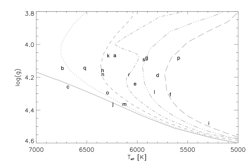
Figure 2: A zoom in on figure 1 with the indvidual stars marked with unique letters.

Figure 3: Separation between the two emission lines in the Ca K₂ core of the K and H lines ($W_{0}$) as a function of effective temperature (see e.g. Ayres, 1979, for definition of this separation). The isochrone tracks are the same as in Fig. 1.

Figure 4: Fraction of the flux in the 1Å bandpass lying within the core of the K and H lines for stars with solar activity levels (bottom line) and up to 8 times solar level.

Figure 5: Measured mean excess fluxes corrected for contribution from the photosphere plotted as function of effective temperature. The solid line shows the relation for the basal flux used in this study.

Figure 6: Relation between the estimated equatorial velocities measured in the $Kepler$ light curves and the $v\sin i$ values from Bruntt et al. (2012). The rotation periods have been scaled with the asteroseismic radii in order to put the two quantities on the same scale. The solid line shows a 1:1 relation. As expected some points are seen above the line. This is partly due to the fact that stars come with random inclinations and partly due to the fact that stars have differential rotation (see text). The dashed line illustrates this by showing the relation for a most probable $v\sin i$ value of $\pi/4$ (Gray, 1992). The diamond represents the Sun.

Figure 7: The relation between the $S$ index and the excess flux $\Delta\mathcal{F}_{\rm Ca}$. A nice log-linear relation is seen between the two quantities except for KIC 8006161.

Figure 8: The relative variability of the excess flux as a function of the mean value of the magnetic emission.

Figure 9: The relative variability of the excess flux as a function of the mean value of the $S$ index.

Figure 10: Histogram of the measured mean magnetic emissions.

Figure 11: Histogram of the measured mean $S$ indicies.

Figure 12: Measured mean excess flux as a function of rotation period. The solid line gives the following log-linear relation: $\log\Delta\mathcal{F}_{\rm Ca}=(-0.74\pm 0.03)\log P_{\rm rot}+6.55\pm 0.02$. The diamond represents the Sun and the dashed line shows the log-linear relation from Skumanich (1972).

Figure 13: Measured mean excess flux as a function of stellar age. The solid line gives the following log-linear relation: $\log\Delta\mathcal{F}_{\rm Ca}=(-0.61\pm 0.17)\log{\rm Age}+6.08\pm 0.13$. The diamond represents the Sun and the dashed line shows the log-linear relation from Skumanich (1972).

Figure 14: Rotation period as a function of age. The solid line gives the following log-linear relation: $\log P_{\rm rot}=(0.45\pm 0.19)\log{\rm Age}+0.59\pm 0.29$. The diamond represents the Sun and the dashed line shows the log-linear relation from Skumanich (1972). The reduced $\chi^{2}$ value of the fit is 2.57.

Figure 15: Rotation period as a function of age and $B-V$ colour. The solid line gives the following log-linear relation: $\log P_{\rm rot}=(0.81\pm 0.10)\log{\rm Age}+\log f(B-V)+0.47\pm 0.22$. The diamond represents the Sun. The reduced $\chi^{2}$ value of the fit is 1.46 – indicating that the colour term in the model is real.

Figure 16: Periodograms of the stars showing rotational modulation of their light curves. There arrows indicates the adopted rotation period. The adopted period is identical to the highest peak in all the periodograms.

References

- Allain et al. (1996) Allain, S., Bouvier, J., Prosser, C., Marschall, L. A., & Laaksonen, B. D. 1996, A&A, 305, 498
- Alonso et al. (1996) Alonso, A., Arribas, S., & Martinez-Roger, C. 1996, A&A, 313, 873
- Appourchaux et al. (2012) Appourchaux, T., Chaplin, W. J., García, R. A., et al. 2012, A&A, 543, A54
- Appourchaux et al. (2008) Appourchaux, T., Michel, E., Auvergne, M., et al. 2008, A&A, 488, 705
- Ayres (1979) Ayres, T. R. 1979, ApJ, 228, 509
- Baliunas & Vaughan (1985) Baliunas, S. L., & Vaughan, A. H. 1985, ARA&A, 23, 379
- Baliunas et al. (1995) Baliunas, S. L., Donahue, R. A., Soon, W. H., et al. 1995, ApJ, 438, 269
- Barnes (2001) Barnes, S. A. 2001, ApJ, 561, 1095
- Barnes (2003) Barnes, S. A. 2003, ApJ, 586, 464
- Barnes (2007) Barnes, S. A. 2007, ApJ, 669, 1167
- Barnes (2010) Barnes, S. A. 2010, ApJ, 722, 222
- Barnes et al. (1999) Barnes, S. A., Sofia, S., Prosser, C. F., & Stauffer, J. R. 1999, ApJ, 516, 263
- Benz et al. (1984) Benz, W., Mayor, M., & Mermilliod, J. C. 1984, A&A, 138, 93
- Bertelli et al. (2008) Bertelli, G., Girardi, L., Marigo, P., & Nasi, E. 2008, A&A, 484, 815
- Bonatto et al. (2004) Bonatto, C., Bica, E., & Girardi, L. 2004, A&A, 415, 571
- Brandenburg et al. (1998) Brandenburg, A., Saar, S. H., & Turpin, C. R. 1998, ApJ, 498, L51
- Brown et al. (2011) Brown, T. M., Latham, D. W., Everett, M. E., & Esquerdo, G. A. 2011, AJ, 142, 112
- Bruntt et al. (2012) Bruntt, H., Basu, S., Smalley, B., et al. 2012, MNRAS, 423, 122
- Böhm-Vitense (2007) Böhm-Vitense, E. 2007, ApJ, 657, 486
- Campante et al. (2010) Campante, T. L., Karoff, C., Chaplin, W. J., et al. 2010, MNRAS, 408, 542
- Chaplin et al. (2010) Chaplin, W. J., et al. 2010, ApJ, 713, L169
- Chaplin et al. (2011a) Chaplin, W. J., Bedding, T. R., Bonanno, A., et al. 2011a, ApJ, 732, L5
- Chaplin et al. (2011b) Chaplin, W. J., Kjeldsen, H., Christensen-Dalsgaard, J., et al. 2011b, Science, 332, 213
- Christensen-Dalsgaard (2008) Christensen-Dalsgaard, J. 2008, Ap&SS, 316, 13
- Donahue (1998) Donahue, R. A. 1998, Cool Stars, Stellar Systems, and the Sun, 154, 1235
- Duncan et al. (1991) Duncan, D. K., Vaughan, A. H., Wilson, O. C., et al. 1991, ApJS, 76, 383
- Durney et al. (1981) Durney, B. R., Mihalas, D., & Robinson, R. D. 1981, PASP, 93, 537
- Elsworth et al. (1995) Elsworth, Y., Howe, R., Isaak, G. R., et al. 1995, A&A supp., 113, 379
- Fletcher et al. (2010) Fletcher, S. T., Broomhall, A.-M., Salabert, D., et al. 2010, ApJ, 718, L19
- Frandsen & Lindberg (2000) Frandsen, S., & Lindberg, B. 2000, The Third MONS Workshop: Science Preparation and Target Selection, 163
- Gabriel et al. (1995) Gabriel, A. H., Grec, G., Charra, J., et al. 1995, Solar Physics, 162, 61
- García et al. (2010) García, R. A., Mathur, S., Salabert, D., et al. 2010, Science, 329, 1032
- Gilliland et al. (2010) Gilliland, R. L., Jenkins, J. M., Borucki, W. J., et al. 2010, ApJ, 713, L160
- Girardi et al. (2002) Girardi, L., Bertelli, G., Bressan, A., Chiosi, C., Groenewegen, M. A. T., Marigo, P., Salasnich, B., & Weiss, A. 2002, A&A, 391, 195
- Girardi et al. (2004) Girardi, L., Grebel, E. K., Odenkirchen, M., & Chiosi, C. 2004, A&A, 422, 205
- Gray (1992) Gray, D. F. 1992, Camb. Astrophys. Ser.
- Gray et al. (2003) Gray, R. O., Corbally, C. J., Garrison, R. F., McFadden, M. T., & Robinson, P. E. 2003, AJ, 126, 2048
- Gray et al. (2006) Gray, R. O., Corbally, C. J., Garrison, R. F., et al. 2006, AJ, 132, 161
- Hall (2008) Hall, J. C. 2008, Living Reviews in Solar Physics, 5, 2
- Hall & Lockwood (1995) Hall, J. C., & Lockwood, G. W. 1995, ApJ, 438, 404
- Hall et al. (2007) Hall, J. C., Lockwood, G. W., & Skiff, B. A. 2007, AJ, 133, 862
- Hartman et al. (2009) Hartman, J. D., Gaudi, B. S., Pinsonneault, M. H., et al. 2009, ApJ, 691, 342
- Hathaway et al. (1996) Hathaway, D. H., Gilman, P. A., Harvey, J. W., et al. 1996, Science, 272, 1306
- Henry et al. (1996) Henry, T. J., Soderblom, D. R., Donahue, R. A., & Baliunas, S. L. 1996, AJ, 111, 439
- Holzwarth & Jardine (2005) Holzwarth, V., & Jardine, M. 2005, A&A, 444, 661
- Høg et al. (2000) Høg, E., Fabricius, C., Makarov, V. V., et al. 2000, A&A, 355, L27
- Isaacson & Fischer (2010) Isaacson, H., & Fischer, D. 2010, ApJ, 725, 875
- Judge et al. (2004) Judge, P. G., Saar, S. H., Carlsson, M., & Ayres, T. R. 2004, ApJ, 609, 392
- Karoff (2008) Karoff C., 2008, PhD dissertation, Aarhus University
- Karoff et al. (2009) Karoff, C., Metcalfe, T. S., Chaplin, W. J., et al. 2009 (CK09), MNRAS, 399, 914
- Karoff et al. (2010a) Karoff, C., Campante, T. L., & Chaplin, W. J. 2010a, arXiv:1003.4167
- Karoff et al. (2010b) Karoff, C., Chaplin, W. J., Appourchaux, T., et al. 2010b, Astronomische Nachrichten, 331, 972
- Kawaler (1988) Kawaler, S. D. 1988, ApJ, 333, 236
- van Leeuwen & Alphenaar (1982) van Leeuwen, F., & Alphenaar, P. 1982, The Messenger, 28, 15
- Lomb (1976) Lomb, N. R. 1976, Ap & SS, 39, 447
- Lutz & Pagel (1982) Lutz, T. E., & Pagel, B. E. J. 1982, MNRAS, 199, 1101
- Mamajek & Hillenbrand (2008) Mamajek, E. E., & Hillenbrand, L. A. 2008, ApJ, 687, 1264
- McQuillan et al. (2012) McQuillan, A., Aigrain, S., & Roberts, S. 2012, A&A, 539, A137
- Meibom et al. (2011a) Meibom, S., Barnes, S. A., Latham, D. W., et al. 2011a, ApJ, 733, L9
- Meibom et al. (2011b) Meibom, S., Mathieu, R. D., Stassun, K. G., Liebesny, P., & Saar, S. H. 2011b, ApJ, 733, 115
- Metcalfe et al. (2010) Metcalfe, T. S., Basu, S., Henry, T. J., et al. 2010, ApJ, 723, L213
- Middelkoop (1982) Middelkoop, F. 1982, A&A, 107, 31
- Nielsen & Karoff (2012) Nielsen, M. B., & Karoff, C. 2012, Astronomische Nachrichten, 333, 1036
- Nielsen et al. (2013) Nielsen, M. B., Gizon, L., Schunker, H., & Karoff, C. 2013, arXiv:1305.5721
- Noyes et al. (1984) Noyes, R. W., Hartmann, L. W., Baliunas, S. L., Duncan, D. K., & Vaughan, A. H. 1984, ApJ, 279, 763
- Pinsonneault et al. (1990) Pinsonneault, M. H., Kawaler, S. D., & Demarque, P. 1990, ApJS, 74, 501
- Quirion et al. (2010) Quirion, P.-O., Christensen-Dalsgaard, J., & Arentoft, T. 2010, ApJ, 725, 2176
- Roxburgh (2009) Roxburgh, I. W. 2009, A&A, 506, 435
- Rutten (1984) Rutten, R. G. M. 1984, A&A, 130, 353
- Rutten & Schrijver (1987) Rutten, R. G. M., & Schrijver, C. J. 1987, A&A, 177, 155
- Saar & Brandenburg (1999) Saar, S. H., & Brandenburg, A. 1999, ApJ, 524, 295
- Salabert et al. (2011) Salabert, D., Régulo, C., Ballot, J., García, R. A., & Mathur, S. 2011, A&A, 530, A127
- Schou et al. (1998) Schou, J., et al. 1998, ApJ, 505, 390
- Schrijver (1995) Schrijver, C. J. 1995, A&ARv, 6, 181
- Schrijver et al. (1989) Schrijver, C. J., Dobson, A. K., & Radick, R. R. 1989, ApJ, 341, 1035
- Schrijver & Zwaan (2008) Schrijver, C. J., & Zwaan, C. 2008, Solar and Stellar Magnetic Activity, by C. J. Schrijver , C. Zwaan, Cambridge, UK: Cambridge University Press, 2008,
- Skumanich (1972) Skumanich, A. 1972, ApJ, 171, 565
- Skumanich & MacGregor (1986) Skumanich, A., & MacGregor, K. 1986, Advances in Space Research, 6, 151
- Soderblom et al. (1991) Soderblom, D. R., Duncan, D. K., & Johnson, D. R. H. 1991, ApJ, 375, 722
- Soderblom & Mayor (1993) Soderblom, D. R., & Mayor, M. 1993, ApJ, 402, L5
- Soderblom et al. (2001) Soderblom, D. R., Jones, B. F., & Fischer, D. 2001, ApJ, 563, 334
- Stauffer et al. (1985) Stauffer, J. R., Hartmann, L. W., Burnham, J. N., & Jones, B. F. 1985, ApJ, 289, 247
- Terndrup et al. (2002) Terndrup, D. M., Pinsonneault, M., Jeffries, R. D., et al. 2002, ApJ, 576, 950
- Vaughan & Preston (1980) Vaughan, A. H., & Preston, G. W. 1980, PASP, 92, 385
- Verner et al. (2011) Verner, G. A., Chaplin, W. J., Basu, S., et al. 2011, ApJ, 738, L28
- Wilson (1978) Wilson, O. C. 1978, ApJ, 226, 379
- Wright et al. (2004) Wright, J. T., Marcy, G. W., Butler, R. P., & Vogt, S. S. 2004, ApJ, 152, 261