Aggregation and long memory: recent developments

Abstract

It is well-known that the aggregated time series might have very different properties from those of the individual series, in particular, long memory. At the present time, aggregation has become one of the main tools for modelling of long memory processes. We review recent work on contemporaneous aggregation of random-coefficient AR(1) and related models, with particular focus on various long memory properties of the aggregated process.

Keywords: Random-coefficient AR(1); contemporaneous aggregation; long memory; infinite variance; mixed moving average; scaling limit; intermediate process; autoregressive random fields; anisotropic long memory; disaggregation.

1 Introduction

In the seminal paper [1980] observed that the covariance function of AR(1) process with random and Beta distributed coefficient may decay very slowly as in ARFIMA process. Indeed, let $X(t)=\sum_{j=0}^{\infty}a^{j}\zeta(t-j)$ be a stationary solution of AR(1) equation

$$X(t)=aX(t-1)+\zeta(t),\quad t\in\mathbb{Z},$$ (1.1)

where $\{\zeta(t)\}\sim WN(0,\sigma^{2})$ is a white noise and $a\in[0,1)$ is a r.v., independent of $\{\zeta(t)\}$, and having a density $\phi(x)$ regularly varying at the unit root $x=1$, viz.,

$$\phi(x)\sim c_{\phi}(1-x)^{\beta},\quad x\nearrow 1,$$ (1.2)

where $c_{\phi}>0$ and $\beta>-1$ some constants. Assume $0<\beta<1$ in the rest of this section. Then, as $t\to\infty$,

$$\mathrm{E}X(0)X(t) = \sigma^{2}\int_{0}^{1}\frac{x^{t}}{1-x^{2}}\phi(x){{\rm{d}}}x\ \sim\ c\,t^{-\beta},$$ (1.3)

with $c=\sigma^{2}(c_{\phi}/2)\Gamma(\beta)$ with $\Gamma(\beta)=\int_{0}^{\infty}{{\rm e}}^{-y}y^{\beta-1}{{\rm{d}}}y$. In the case of Beta-type density $\phi(x)=\frac{2}{B(p,q)}x^{2p-1}(1-x^{2})^{q-1}$ discussed in [1980], condition (1.2) is satisfied with $\beta=q-1$ and the covariance in (1.3) can be explicitly computed: $\mathrm{E}X(0)X(t)=(\sigma^{2}\Gamma(q-1)/B(p,q))\Gamma(p+\frac{t}{2})/\Gamma(p+\frac{t}{2}+q-1)$, leading to the asymptotics in (1.3) since $\Gamma(t)/\Gamma(t+b)\sim t^{-b}$, $t\to\infty$.

Now suppose that one wants to study a huge and heterogeneous population of dynamic “micro-agents” who all evolve independently of each other according to AR(1) process. Thus, the probability law of the evolution of a given “micro-agent” is completely determined by the value of the autoregressive parameter $a$. The heterogeneity of “micro-agents” means that $a$ has a probability density $\phi$ across the population. The “macroeconomic” variable $\mathfrak{X}_{N}(t)$ of interest is obtained by averaging the evolutions of $N$ “microeconomic” variables $X_{i}(t),i=1,\dots,N$,

$$\mathfrak{X}_{N}(t)\ =\ \frac{1}{A_{N}}\sum_{i=1}^{N}X_{i}(t),\quad t=0,\pm 1,\dots,$$ (1.4)

which are randomly sampled from all “micro-agents” population, where $A_{N}$ is a normalization and $\{X_{i}(t)\},i=1,2,\dots$ are i.i.d. copies of (1.1). By the independence of the summands in (1.4) and the classical CLT, it immediately follows (with $A_{N}=N^{1/2}$) that

$$\mathfrak{X}_{N}(t)\ \stackrel{{\scriptstyle\rm fdd}}{{\rightarrow}}\ \mathfrak{X}(t),$$ (1.5)

where $\{\mathfrak{X}(t)\}$ is a stationary Gaussian process with the same 2nd moment characteristics as the individual “micro-agents”, i.e.

$$\mathrm{E}\mathfrak{X}(t)\ =\ 0,\qquad\mathrm{E}\mathfrak{X}(0)\mathfrak{X}(t)\ =\ \mathrm{E}X(0)X(t)\ =\ \sigma^{2}\int_{0}^{1}\frac{x^{t}}{1-x^{2}}\phi(x){{\rm{d}}}x$$ (1.6)

and where $\stackrel{{\scriptstyle\rm fdd}}{{\rightarrow}}$ denotes the weak convergence of finite-dimensional distributions. In particular, under the assumption (1.2), $0<\beta<1$, the covariance $\mathrm{E}\mathfrak{X}(0)\mathfrak{X}(t)$ decays as in (1.3), implying that $\sum_{t\in\mathbb{Z}}|\mathrm{E}\mathfrak{X}(0)\mathfrak{X}(t)|=\infty,$ i.e., $\{\mathfrak{X}(t)\}$ has long memory. Notice also that the Gaussian process $\{\mathfrak{X}(t)\}$ in (1.5) is ergodic, in contrast to the non-ergodic random-coefficient individual processes $\{X_{i}(t)\}$ in (1.4). Since (1.4) refers to summation of (independent) processes at instant time $t$, the summation procedure (1.4) is called contemporaneous or cross-sectional aggregation, to be distinguished from temporal aggregation, the latter term usually referring to the summation on disjoint successive blocks, or taking partial sums, of a single time series. We see that contemporaneous aggregation of simple dynamic models can result in a long memory process and hence may provide an explanation of the long memory phenomenon observed in many econometric studies ([1996], [2007]). The last fact is very important since economic reasons of long memory remain largely unclear and some authors try explain this phenomenon by “spurious long memory” ([1998], [2003]).

It is also instructive to look at the behavior (1.3) from the “spectral perspective”. The spectral density of the random-coefficient AR(1) process is written as

$$f(y)=\frac{\sigma^{2}}{2\pi}\int_{0}^{1}\frac{1}{|1-x{\rm e}^{{\rm i}y}|^{2}}\phi(x){\rm{d}}x=\frac{\sigma^{2}}{2\pi}\int_{0}^{1}\frac{1}{(1-x)^{2}+4x\sin^{2}(y/2)}\phi(x){\rm{d}}x,\quad y\in[-\pi,\pi].$$

We see that under (1.2), $0<\beta<1$, when $y\searrow 0$, this “aggregated” spectral density behaves like a power function:

$$f(y) \sim \sigma^{2}\frac{c_{\phi}}{2\pi}\int_{0}^{1}\frac{(1-x)^{\beta}{\rm{d}}x}{(1-x)^{2}+4x\sin^{2}(y/2)}\ \sim\ \sigma^{2}\frac{c_{\phi}}{2\pi}\int_{0}^{1}\frac{x^{\beta}\,{\rm{d}}x}{x^{2}+4\sin^{2}(y/2)}$$ (1.7)

$$= \sigma^{2}\frac{c_{\phi}}{2\pi(2\sin(y/2))^{1-\beta}}\int_{0}^{1/2\sin(y/2)}\frac{w^{\beta}{\rm{d}}w}{w^{2}+1}$$

$$\sim \frac{c_{f}}{y^{1-\beta}},$$

where $c_{f}:=\sigma^{2}\frac{c_{\phi}}{2\pi}\int_{0}^{\infty}\frac{w^{\beta}{\rm{d}}w}{w^{2}+1}$. The singularity in the low frequency spectrum of $\{X(t)\}$ and $\{\mathfrak{X}(t)\}$ is another indication of long memory of these processes and is not surprising as the power behaviors (1.3) and (1.7) are known to be roughly equivalent. Relation (1.7) seems to be well-known to physicists and even experimentally observed, relating aggregation and long memory to the vast area in physics called $1/f$ noise (see, e.g., the article by Ward and Greenwood (?) in Scholarpedia). Another manifestation of long memory for the aggregated process in (1.7) is the convergence of normalized partial sums of $\{\mathfrak{X}(t)\}$ to a fractional Brownian motion ([2004]). See Sec. 2 for the related notion of distributional long memory.

Following [1980], various aspects of aggregation were discussed in the literature, see [1988], Zaffaroni (?, ?), [2004], [2006], Celov et al. (?, ?), [2011]. [2004] considered aggregation of general AR($2p)$ processes with $2p$ random coefficients, under the condition that the characteristic polynomial has the form

$$A(z)\ =\ (1-\alpha_{1}z)(1+\alpha_{2}z)\prod_{k=3}^{p+1}(1-\alpha_{k}{\rm e}^{{\rm i}\theta_{k}}z)(1-\alpha_{k}{\rm e}^{-{\rm i}\theta_{k}}z),$$

where $\alpha_{1},\dots,\alpha_{p+1}$ are i.i.d. random variables with probability densities as in (1.2), with (possibly) different $\beta$’s, and $\theta_{3},\dots,\theta_{p+1}$ are fixed. They described the singularities of the spectral density and the asymptotics of the covariance function of the corresponding aggregated Gaussian process, which may contain a seasonal component. [2004] considered a general aggregation scheme of random-coeffcient AR(1) with idiosyncratic and common components. Several papers ([1996], [2007a], [2007b], [2002], [2004], [2010]) extended the aggregation scheme to ARCH-type heteroskedastic processes with random coeffcients and common innovations, with a particular emphasis on long memory behavior. The disaggregation problem of reconstructing the mixing distribution from the spectral density or observed sample from the aggregated process and its statistical aspects were studied [2006], [2007], [2006], [2010], [2011], [1978], [2010] and elsewhere. Some aspects of aggregation and disaggregation are also discussed in the recent monograph [2013].

The aim of the present paper is to review recent developments on aggregation and long memory. Sec. 2 discusses the case of AR(1) processes with infinite variance. Sec. 3 extends the aggregation procedure to the triangular array model. Sec. 4 studies the joint temporal ant contemporaneous aggregation of AR(1) processes. Sec. 5 considers the aggregation procedure for random fields. Sec. 6 reviews some results related to statistical inference for the mixing density $\phi$.

2 Aggregation of AR(1) processes with infinite variance

The approach of [1980] presented Sec. 1 can be extended to the case of infinite variance. Let

$$X(t)\ =\ \sum_{j=0}^{\infty}a^{j}\zeta(t-j)$$ (2.1)

be a stationary solution of the AR(1) equation (1.1) with random coefficient $a\in[0,1)$ and i.i.d. innovations $\{\zeta(t)\}$ with infinite variance ${\rm Var}(\zeta(t))=\infty$, independent of r.v. $a$, and belonging to the domain of attraction of $\alpha-$stable law, $0<\alpha<2$, in the sense that

$$\frac{1}{N^{1/\alpha}}\sum_{i=1}^{N}\zeta(i)\ \stackrel{{\scriptstyle\rm d}}{{\rightarrow}}\ Z,$$ (2.2)

where $Z$ is an $\alpha-$stable r.v. Let $\{X_{i}(t)\},i=1,2,\dots$ be independent copies of (2.1), and define the aggregated process as

$$\mathfrak{X}_{N}(t)\ :=\ \frac{1}{N^{1/\alpha}}\sum_{i=1}^{N}X_{i}(t),\quad t\in\mathbb{Z}.$$ (2.3)

The problem is to determine the limit process $\{\mathfrak{X}(t)\}$ of (2.3), in the sense of (1.5), and then we describe its properties, in particular, long memory properties.

The above questions were studied in [2010]. Note that the AR(1) series in (2.1) converges conditionally a.s. for every $a\in[0,1)$, and also unconditionally a.s. if the distribution of $a$ satisfies the additional condition $\mathrm{E}(1-a)^{-1}<\infty.$ For regularly varying $\phi$ as in (1.2), the last condition is equivalent to $\beta>0$. It is shown in Puplinskaitė and Surgailis (?, Thm. 2.1) that in the case $\beta>0$ the limit of $\{\mathfrak{X}_{N}(t)\}$ exists and is written as a stochastic integral

$$\mathfrak{X}(t)\ :=\ \sum_{s\leq t}\int_{[0,1)}x^{t-s}M_{\alpha,s}({{\rm{d}}}x),$$ (2.4)

where $\{M_{\alpha,s},s\in\mathbb{Z}\}$ are i.i.d. copies of an $\alpha-$stable random measure on $[0,1)$ with distribution $Z$ in (2.2) and control measure equal to the mixing distribution $\Phi$ (i.e., the distribution of the r.v. $a$). Recall that a family $M=\{M(A),A\in{\cal B}_{0}(S)\}$ of r.v.’s indexed by sets $A\in{\cal B}_{0}(S):=\{A\in{\cal B}(S):\mu(A)<\infty\}$ of a measure space $(S,{\cal B}(S),\mu)$ with a $\sigma-$finite measure $\mu$ is called a random measure with distribution $W$ and control measure $\mu$ (where $W$ is an infinitely divisible r.v.) if for any disjoint sets $A_{i}\in{\cal B}_{0}(S)$, $i=1,\dots,n$, $n\geq 1$ r.v.’s $M(A_{i}),i=1,\dots,n$ are independent, $M(\cup_{i=1}^{n}A_{i})=\sum_{i=1}^{n}M(A_{i})$, and

$$\mathrm{E}{\rm e}^{{\rm i}\theta M(A)}=(\mathrm{E}{\rm e}^{{\rm i}\theta W})^{\mu(A)},\quad\forall A\in{\cal B}_{0}(S),\ \ \forall\theta\in\mathbb{R}.$$

Integration with respect to stable and general infinitely divisible random measures is discussed in [1994], [1989] and other texts. The process in (2.4) is a particularly simple case of the so-called mixed stable moving averages introduced in [1993]. It is stationary, ergodic, and has $\alpha-$stable finite-dimensional distributions. The representation (2.4) of the limit aggregated process holds also in the finite-variance case $\alpha=2$, yielding a stationary Gaussian process with zero mean and covariance

$${\rm Cov}(\mathfrak{X}(0),\mathfrak{X}(t))\ =\ \sigma^{2}\sum_{s\leq 0}\int_{[0,1)}x^{-s}x^{t-s}\Phi({\rm{d}}x)\ =\ \sigma^{2}\mathrm{E}\Big{[}\frac{a^{t}}{1-a^{2}}\Big{]},\quad t=0,1,\dots,$$

cf. (1.3). The mixed stable moving average in (2.4) can be regarded as a limiting “superposition” $\sum_{a_{i}\in[0,1)}{\cal X}(t;a_{i})$ of independent $\alpha-$stable AR(1) processes ${\cal X}(t;a_{i})=\sum_{s\leq t}a_{i}^{t-s}{\cal M}_{\alpha,i}(t-s)$ with $\alpha-$stable innovations $\{{\cal M}_{\alpha,i}(s)\}$. Although each $\{{\cal X}(t;a_{i})\}$ is geometrically mixing and hence short memory, the dependence in $\{{\cal X}(t;a_{i})\}$ increases when $a_{i}\nearrow 1$ approaches the “unit root” $a=1$. It turns out that the limiting “superposition” of these processes and the mixed moving average in (2.4) may have long (or short) memory, depending on the concentration of the $a_{i}$’s near $a=1$, or the parameter $\beta$ in (1.2).

Before addressing the question about long memory of the infinite variance process in (2.4), let us note that the above mentioned convergence of (2.3) to (2.4) does not hold in the case of negative exponent $-1<\beta<0$. It turns out that in the latter case, the limit aggregated process does not depend on $t$ and is an $\alpha(1+\beta)-$stable r.v. (random constant):

$$\frac{1}{N^{1/(\alpha(1+\beta))}}\sum_{i=1}^{N}X_{i}(t)\ \stackrel{{\scriptstyle\rm fdd}}{{\rightarrow}}\ \tilde{Z},$$ (2.5)

see Puplinskaitė and Surgailis (?, Prop. 2.3). In the case $\alpha=2$, a similar result was noted in [2004]. Note that the normalizing exponents $1/\alpha$ in (2.3) and $1/(\alpha(1+\beta))$ in (2.5) are different and $1/(\alpha(1+\beta))\to\infty$ as $\beta\to-1$. Therefore, $\beta=0$ is a critical point resulting in completely different limits of the aggregated process in the cases $\beta>0$ and $\beta<0$. The fact that the limit is degenerate in the latter case can be intuitively explained as follows. It is clear that, with $\beta$ decreasing, the dependence increases in the random-coefficient AR(1) process $\{X(t)\}$, as well as in the limiting aggregated process $\{\mathfrak{X}(t)\}$. For negative $\beta<0$, the dependence in the aggregated process becomes extremely strong so that the limit process is degenerate and completely dependent.

Long memory properties of the limit aggregated process. Clearly, the usual definitions of long memory in terms of covariance/spectrum do not apply in infinite variance case. Alternative notions of long memory which are applicable to infinite-variance processes have been proposed in the literature. [Astrauskas (1983)] was probably the first to rigorously study long memory for such processes in terms of the rate at which the bivariate characteristic function at distant lags factorizes into the product of two univariate characteristic functions. Related characteristics such as codifference are discussed in [1994]. Some characteristics of dependence (covariation, $\alpha$–covariance) for stable processes expressed in terms of the spectral measure were studied in [1994] and [2013]. [1997] defined the long-range dependence (sample Allen variance) (LRD(SAV)) property in terms of the limit behavior of squared studentized sample mean.

Probably, the most useful and universal definition of long/short memory was given by [1984]. Assume that $\{Y(t),t\in\mathbb{Z}\}$ is a strictly stationary process series and there exist some constants $D_{n}\to\infty\ (n\to\infty)$ and $B_{n}$ and a nontrivial stochastic process $J=\{J(\tau),\tau\geq 0\}\not\equiv 0$ such that

$$\frac{1}{D_{n}}\sum_{s=1}^{[n\tau]}(Y(s)-B_{n})\ \stackrel{{\scriptstyle\rm fdd}}{{\rightarrow}}\ J(\tau).$$ (2.6)

According to [1984], if the limit process $J$ has independent increments, the series $\{Y(t)\}$ is said to have distributional short memory, while in the converse case when $J$ has dependent increments, the series $\{Y(t)\}$ is said to have distributional long memory.

The above definition has several advantages. First of all, it does not depend on any moment assumptions since finite and infinite variance processes are treated from the same angle. Secondly, according to the classical Lamperti’s theorem (see [1962]), in the case of (2.6) there exists a number $H>0$ such that the normalizing constants $A_{n}$ grow as $n^{H}$ (modulus a slowly varying factor), while the limit random process $J$ is $H-$self-similar and has stationary increments ($H-$sssi). A faster growth of normalization $A_{n}$ means stronger dependence and therefore $H$ is a quantitative indicator of the degree of dependence in $\{Y(t)\}$. The characterization of short memory through (2.6) is very robust and essentially reduces to Lévy stable behavior since all sssi processes with independent increments are stable Lévy processes. We emphasize that the above definition of long/short memory requires identification of the partial sums limit which is sometimes not easy. On the other hand, partial sums play a very important role in statistical inference, especially under long memory, see e.g. [2012], and hence finding partial sums limit is very natural for understanding the dependence structure of a given process and subsequent applications of statistical nature.

With the above discussion in mind, the question arises what is the partial sums limit of the aggregated process in (2.4)? This question is answered in Puplinskaitė and Surgailis (?, Thm. 3.1) saying that for $1<\alpha\leq 2$ and $0<\beta<\alpha-1$,

$$\frac{1}{n^{1-(\beta/\alpha)}}\sum_{t=1}^{[n\tau]}\mathfrak{X}(t)\ \ \stackrel{{\scriptstyle\rm fdd}}{{\rightarrow}}\ \ \Lambda_{\alpha,\beta}(\tau)\ :=\ \int_{\mathbb{R}_{+}\times\mathbb{R}}(\mathfrak{f}(x,\tau-s)-\mathfrak{f}(x,-s))Z_{\alpha}({\rm{d}}x,{\rm{d}}s),$$ (2.7)

where

$$\mathfrak{f}(x,t)\ :=\ \begin{cases}(1-{{\rm e}}^{-xt})/x,&\text{if}\ x>0\ \text{and}\ t>0,\\ 0,&\text{otherwise},\end{cases}$$ (2.8)

and $Z_{\alpha}({\rm{d}}x,{\rm{d}}s)$ is an $\alpha-$stable random measure on $\mathbb{R}_{+}\times\mathbb{R}$ with control measure $c_{\phi}x^{\beta}{\rm{d}}x\,{\rm{d}}s$ and distribution $Z$, where $Z$ is defined at (2.2). The random process $\Lambda_{\alpha,\beta}$ in (2.7) is well-defined for $1<\alpha\leq 2$, $0<\beta<\alpha-1$ and is $H-$sssi with self-similarity index $H=1-\frac{\beta}{\alpha}\in(\frac{1}{\alpha},1).$ Moreover, $\Lambda_{\alpha,\beta}$ has a.s. continuous paths, $\alpha-$stable finite dimensional distributions and stationary and dependent increments. In particular, $\Lambda_{2,\beta}$ is a fractional Brownian motion with $H=1-\frac{\beta}{2}\in(\frac{1}{2},1).$ The process $\Lambda_{\alpha,\beta}$ is also different from linear fractional Lévy motion (see, e.g., [1994] for a detailed discussion of the latter process).

Similarly as $\{\mathfrak{X}(t)\}$ in (2.4) can be regarded as a “continuous superposition” of AR(1) processes, the limit process $\Lambda_{\alpha,\beta}$ in (2.7) can be regarded as a “continuous superposition” of (integrated) Ornstein-Uhlenbeck processes $z_{\alpha}(\tau;x)$ defined as

$$z_{\alpha}(\tau;x)\ :=\ \int_{0}^{\tau}{\rm{d}}u\int_{\mathbb{R}}{\rm e}^{-x(u-s)}{\bf 1}(u>s){\rm{d}}Z_{\alpha}(s)\ =\ \int_{\mathbb{R}}\big{(}\mathfrak{f}(x,\tau-s)-\mathfrak{f}(x,-s)\big{)}{\rm{d}}Z_{\alpha}(s),\quad\tau\geq 0,\ x>0,$$ (2.9)

where $\{Z_{\alpha}(s),s\geq 0\}$ is an $\alpha-$stable Lévy process with independent increments. Note that for each $x>0$, the process $\{z_{\alpha}(\tau;x)\}$ is a.s. continuously differentiable on $\mathbb{R}$ and its derivative $z^{\prime}_{\alpha}(\tau;x)={\rm{d}}z_{\alpha}(\tau;x)/{\rm{d}}\tau$ satisfies the Langevin equation

$${\rm{d}}z^{\prime}_{\alpha}(\tau;x)\ =\ -xz^{\prime}_{\alpha}(\tau;x){\rm{d}}\tau+{\rm{d}}Z_{\alpha}(\tau).$$

In the case $\alpha=2$, $Z_{2}=B$ is a usual Brownian motion and $z_{2}(\tau;x)$ is a Gaussian Ornstein-Uhlenbeck process. The corresponding representation of $\Lambda_{2,\beta}$ in (2.7) may be termed the Ornstein-Uhlenbeck representation of fractional Brownian motion, and the process $\Lambda_{\alpha,\beta},\,1<\alpha<2$ its stable counterpart. A related class of stationary infinitely divisible processes with long memory is discussed in [2001].

The condition $1<\alpha\leq 2,\,0<\beta<\alpha-1$ for the convergence in (2.7) is sharp and cannot be weakened. In particular, for $\beta>\alpha-1$ the partial sums process $n^{-1/\alpha}\sum_{t=1}^{[n\tau]}\mathfrak{X}(t)$ tends to an $\alpha-$stable Lévy process with independent increments (see Puplinskaitė and Surgailis (?, Thm. 3.1)). Therefore, large sample behaviors of $\{\mathfrak{X}(t)\}$ for $0<\beta<\alpha-1$ and $\beta>\alpha-1$ are markedly different. Following the above terminology, the aggregated AR(1) process $\{\mathfrak{X}(t)\}$ has distributional long memory if $0<\beta<\alpha-1$ and distributional short memory if $\beta>\alpha-1$. In the last case, assumption (1.2) on the mixing distribution can be substantially relaxed.

[2010] also studied other characterizations of long memory of the aggregated AR(1) process $\{\mathfrak{X}(t)\}$ with infinite variance (the LRD(SAV) property, the decay rate of codifference). A curious characterization of long memory in terms of the asymptotic behaviour of the ruin probability in a discrete time risk insurance model with $\alpha-$stable claims $\{\mathfrak{X}(t)\}$ in (2.4) is obtained in [2013], following the characterization studied in [2000]. All these results agree with the above characterization in terms of the partial sums process, in the sense that $\beta=\alpha-1$ is the boundary between long memory and short memory in $\{\mathfrak{X}(t)\}$.

Finally, let us note that the general aggregation scheme of random-coefficient autoregressive processes discussed in [2004] includes the case of common component, or common innovations. Aggregation of infinite variance AR(1) processes with common innovations was studied in [2009]. In this case, the limit aggregated process, say $\{\widetilde{\mathfrak{X}}(t)\}$, exists under normalization $1/N$ and is a moving average with the same innovations as the original AR(1) series (2.1) and the moving average coefficients given by the expectations $\mathrm{E}a^{j}=\int_{[0,1)}x^{j}\Phi({\rm{d}}x)$. By a similar argument as in (1.3), we have that $\mathrm{E}a^{j}\sim const\;j^{-\beta-1}$ for $\beta>-1$. Therefore for $1/\alpha<\beta<0$, $\{\widetilde{\mathfrak{X}}(t)\}$ is a well-defined long memory moving average with infinite variance and nonsummable coefficients $\sum_{j=0}^{\infty}\mathrm{E}a^{j}=\infty$. [2009] investigated various long memory properties of $\{\widetilde{\mathfrak{X}}(t)\}$, including the convergence of its partial sums to a linear fractional Lévy motion.

3 Aggregation of AR(1) processes: triangular array innovations

The contemporaneous aggregation scheme of Sec. 2 can be generalized by assuming that the innovations depend on $N$, constituting a triangular array of i.i.d. r.v.’s. Such aggregation scheme was studied in [2013]. Let $\{X^{(N)}_{i}(t)\}$, $i=1,\dots,N$ be i.i.d. copies of of random-coefficient AR(1) process

$$X^{(N)}(t)\ =\ aX^{(N)}(t-1)+\zeta^{(N)}(t),\quad t\in\mathbb{Z},$$ (3.1)

where $\{\zeta^{(N)}(t),\,t\in\mathbb{Z}\},\,N=1,2,\dots$ is a triangular array of i.i.d. random variables in the domain of attraction of an infinitely divisible law $W$:

$$\sum_{i=1}^{N}\zeta^{(N)}(i) \stackrel{{\scriptstyle\rm d}}{{\rightarrow}} W,$$ (3.2)

and $a\in[0,1)$ is a r.v., independent of $\{\zeta^{(N)}(t),t\in\mathbb{Z}\}$. The limit aggregated process $\{\mathfrak{X}(t),t\in\mathbb{Z}\}$ is defined as the limit in distribution:

$$\sum_{i=1}^{N}X^{(N)}_{i}(t)\ \stackrel{{\scriptstyle\rm fdd}}{{\rightarrow}}\ \mathfrak{X}(t).$$ (3.3)

Sec. 2 corresponds to the particular case of (3.1)–(3.2), viz., $\zeta^{(N)}(t)=N^{-1/\alpha}\zeta(t),$ where $\{\zeta(t),t\in\mathbb{Z}\}$ are i.i.d. r.v.’s in the domain of (normal) attraction of $\alpha-$stable law $W,\,0<\alpha\leq 2.$ In particular, for $\alpha=2$ or $W\sim{\cal N}(0,\sigma^{2})$ the last condition is equivalent to $\mathrm{E}\zeta(t)=0$ and $\sigma^{2}=\mathrm{E}W^{2}<\infty$.

One of the main results of [2013] says that under mild additional conditions the limit in (3.3) exists and is written as a mixed infinitely divisible (ID) moving average (see the terminology in [1989]):

$$\mathfrak{X}(t)\ =\ \sum_{s\leq t}\int_{[0,1)}x^{t-s}M_{W,s}({{\rm{d}}}x),\qquad t\in\mathbb{Z},$$ (3.4)

where $\{M_{W,s},s\in\mathbb{Z}\}$ are i.i.d. copies of an ID random measure $M_{W}$ on $[0,1)$ with control measure $\Phi({\rm{d}}x)=\mathrm{P}(a\in{\rm{d}}x)$ and the distribution $W$ in (3.2). Recall that the last distribution is uniquely determined by its Lévy characteristics $(\mu,\sigma,\pi)$ (the characteristic triplet) since

$$V(\theta) := \log\mathrm{E}{\rm e}^{{\rm i}\theta W}\ =\ \int_{\mathbb{R}}({\rm e}^{{{\rm i}}\theta x}-1-{{\rm i}}\theta x{\bf 1}(|x|\leq 1))\pi({\rm{d}}x)-\frac{1}{2}\theta^{2}\sigma^{2}+{\rm i}\theta\mu,$$ (3.5)

where $\mu\in\mathbb{R},\,\sigma\geq 0$ and $\pi$ is a Lévy measure, see [1994], [1999].

[2013] discuss distributional long/short memory properties of the aggregated process $\{\mathfrak{X}(t)\}$ in (3.4) with finite variance and a mixing density as in (1.2). The finite variance assumption is equivalent to $\mathrm{E}(1-a)^{-1}<\infty$ and

$$\sigma^{2}_{W}\ :=\ {\rm Var}(W)<\infty\qquad\Longleftrightarrow\qquad\int_{\mathbb{R}}x^{2}\pi({\rm{d}}x)<\infty.$$ (3.6)

Note that (3.6) excludes the $\alpha-$stable case discussed in the previous sec. Under (3.6) the covariance function of (3.4) is written as in the Gaussian case (1.6), with $\sigma^{2}$ replaced by $\sigma^{2}_{W}$. Therefore the covariance asymptotics in (1.3) applies also for the process $\{\mathfrak{X}(t)\}$ in (3.4), yielding

$${\rm Var}\Big{(}\sum_{t=1}^{n}\mathfrak{X}(t)\Big{)}\ \sim\ Cn^{2-\beta},\qquad 0<\beta<1.$$ (3.7)

From (3.7) and the linear structure of $\{\mathfrak{X}(t)\}$ one might expect a Gaussian (fractional Brownian motion) limit behavior of the partial sums process $S_{n}(\tau)=\sum_{t=1}^{[n\tau]}\mathfrak{X}(t)$.

However, as it turns out, the Gaussian scenario for $\{S_{n}(\tau)\}$ is valid only if $\sigma>0$ in (3.5), or the Gaussian component is present in the ID r.v. $W$. Else (i.e., when $\sigma=0$), the behavior of the Lévy measure $\pi$ at the origin plays a dominant role. Assume that there exist $\alpha_{0}>0$ and $c^{\pm}_{0}\geq 0,c^{+}_{0}+c^{-}_{0}>0$ such that

$$\lim_{x\searrow 0}x^{\alpha_{0}}\pi(x,\infty)=c^{+}_{0},\qquad\lim_{x\searrow 0}x^{\alpha_{0}}\pi(-\infty,-x)=c^{-}_{0}.$$ (3.8)

It is proved in [2013] that under conditions (1.2), (3.6), and (3.8), partial sums $\{S_{n}(\tau)\}$ of $\{\mathfrak{X}(t)\}$ in (3.4) may exhibit at least four different limit behaviors, depending on parameters $\beta,\sigma,$ and $\alpha_{0}$. The four parameter regions and the limit behaviors in the f.d.d. sense are described in (i)–(iv) below.

(i)

$0<\beta<1,\ \sigma>0.$ In this region, $\ n^{(\beta/2)-1}S_{n}(\tau)\$ tends to a fractional Brownian motion with Hurst parameter $H=1-(\beta/2).$

(ii)

$0<\beta<1,\ \sigma=0,\ 1+\beta<\alpha_{0}<2.$ In this region, $\ n^{(\beta/\alpha_{0})-1}S_{n}(\tau)\$ tends to the $\alpha_{0}-$stable self-similar process $\Lambda_{\alpha_{0},\beta}$ defined in (2.7).

(iii)

$0<\beta<1,\ \sigma=0,\ 0<\alpha_{0}<1+\beta.$ In this region, $\ n^{-1/(1+\beta)}S_{n}(\tau)\$ tends to a $(1+\beta)-$stable Lévy process with independent increments.

(iv)

$\beta>1.$ In this region, $\ n^{-1/2}S_{n}(\tau)\$ tends to a Brownian motion.

See [2013] for precise formulations. Accordingly, the process $\{\mathfrak{X}(t)\}$ in (3.4) has distributional long memory in regions (i) and (ii) and distributional short memory in regions (iii) and (iv). As $\alpha_{0}$ increases from $0$ to $2$, the Lévy measure in (3.8) increases its “mass” near the origin, the limiting case $\alpha_{0}=2$ corresponding to $\sigma>0$ or a positive “mass” at $0$. We see from (i)–(ii) that distributional long memory is related to $\alpha_{0}$ being large enough, or small jumps of the random measure $M_{W}$ having sufficient high intensity. Note that the critical exponent $\alpha_{0}=1+\beta$ separating the long and short memory “regimes” in (ii) and (iii) decreases with $\beta,$ which is quite natural since smaller $\beta$ means the mixing distribution putting more weight near the unit root $a=1$.

Let us note that an $\alpha-$stable limit behavior of partial sums of stationary finite variance processes is not unusual under long memory. See, e.g., [1997], [2002], [2003] and the references herein. On the other hand, these papers focus on heavy-tailed duration models in which case the limit $\alpha-$stable process has independent increments as a rule. The situation when an infinite variance limit process with dependent increments arises from partial sums of a finite variance process as in (ii) above seems rather new.

4 Joint temporal and contemporaneous aggregation of AR(1) processes

The aggregation procedures discussed in the previous sec. extend in a natural way to the (large scale) joint temporal and contemporaneous aggregation. In the latter frame, we are interested in the limit behavior of the double sums

$$S_{N,n}(\tau)\ :=\ \sum_{i=1}^{N}\sum_{t=1}^{[n\tau]}X_{i}(t),\quad\tau\geq 0,$$ (4.1)

where $\{X_{i}(t)\},i=1,\dots,N$ are the same random-coefficient AR(1) processes as in (1.4). The sum in (4.1) represents joint temporal and contemporaneous aggregate of $N$ individual AR(1) evolutions at time scale $n$. The main question is the joint aggregation limit $\lim_{N,n\to\infty}A^{-1}_{N,n}S_{N,n}(\tau)$, in distribution, where $A_{N,n}$ are some normalizing constants and both $N$ and $n$ increase to infinity, possibly at different rate. This question was studied in [2013]. The last paper also discussed the iterated limits of $A^{-1}_{N,n}S_{N,n}(\tau)$ when first $n\to\infty$ and then $N\to\infty$, or vice-versa. Remark that the discussion in the previous sec. refers to the latter iterated limit as $N\to\infty$ first, followed by $n\to\infty$. Similar questions for some network traffic models were studied in [1997], [2002], [2003], [2004], [2011] and other papers. In these papers, the role of AR(1) processes $\{X_{i}(t)\}$ in (4.1) play independent ON/OFF processes or M/G/$\infty$ queues with heavy-tailed activity periods.

Let us describe the main results in [2013]. They refer to the random-coefficient AR(1) process with i.i.d. innovations having zero mean and variance $\sigma^{2}<\infty$, and a mixing density as (1.2). Let $N,n$ increase simultaneously so as

$$\frac{N^{1/(1+\beta)}}{n}\ \to\ \mu\,\in\,[0,\infty],$$ (4.2)

leading to the following three cases:

$$\text{Case (j)}:\ \mu=\infty,\qquad\text{Case (jj)}:\ \mu=0,\qquad\text{Case (jjj)}:\ 0<\mu<\infty.$$ (4.3)

Following the terminology in [2002] and [2004], we call Cases (j), (jj), and (jjj) the “fast growth condition” , the “slow growth condition”, and the “intermediate growth condition”, respectively, since they reflect how fast $N$ grows with $n$. The main result of [2013] says that under (4.2), the “simultaneous limit” of $S_{N,n}(\tau)$ exist and are different in all three Cases (j)–(jjj).

Case (j) (the “fast growth condition”): For any $0<\beta<1$,

$$N^{-1/2}n^{-1+(\beta/2)}S_{N,n}(\tau)\ \stackrel{{\scriptstyle\rm fdd}}{{\rightarrow}}\ B_{1-\beta/2}(\tau),$$ (4.4)

where $\{B_{1-\beta/2}(\tau)\}$ is a fractional Brownian motion with $H=1-\beta/2\in(1/2,1)$.

Case (jj) (the “slow growth condition”): For any $-1<\beta<1$,

$$N^{-1/(1+\beta)}n^{-1/2}S_{N,n}(\tau)\ \stackrel{{\scriptstyle\rm fdd}}{{\rightarrow}}\ {\cal W}_{\beta}(\tau),$$ (4.5)

where $\{{\cal W}_{\beta}(\tau)\}$ is a sub-Gaussian $(1+\beta)-$stable process defined as ${\cal W}_{\beta}(\tau)=W_{\beta}^{1/2}B(\tau),\,\tau\geq 0$, where $W_{\beta}>0$ is a $(1+\beta)/2-$stable totally skewed r.v. and $\{B(\tau),\tau\geq 0\}$ is a standard Brownian motion independent of $W_{\beta}$ (see, e.g., [1994]).

Case (jjj) (the “intermediate growth condition”): For any $-1<\beta<1$

$$N^{-1/(1+\beta)}n^{-1/2}S_{N,n}(\tau)\ \stackrel{{\scriptstyle\rm fdd}}{{\rightarrow}}\ \mu^{1/2}{\cal Z}_{\beta}(\tau/\mu),$$ (4.6)

where the limit process $\{{\cal Z}_{\beta}(\tau),\tau\geq 0\}$ is defined through finite-dimensional characteristic function:

$$\mathrm{E}\exp\Big{\{}{\rm i}\sum_{j=1}^{m}\theta_{j}{\cal Z}_{\beta}(\tau_{j})\Big{\}} = \exp\Big{\{}c_{\phi}\int_{\mathbb{R}_{+}}\big{(}{\rm e}^{-(\sigma^{2}/2)\int_{\mathbb{R}}\big{(}\sum_{j=1}^{m}\theta_{j}(\mathfrak{f}(x,\tau_{j}-s)-\mathfrak{f}(x,-s))\big{)}^{2}{\rm{d}}s}-1\big{)}x^{\beta}{\rm{d}}x\Big{\}},$$ (4.7)

where $\theta_{j}\in\mathbb{R},\tau_{j}\in\mathbb{R}_{+},j=1,\dots,m,\,m\geq 1,$ and $\mathfrak{f}$ is given in (2.8).

Let us give some comments on the above results. The convergence in Case (j) (4.4) is very natural in view of (2.7) (with $\alpha=2$ and $\Lambda_{2,\beta}=B_{1-\beta/2}$ a fractional Brownian motion). Indeed, under the “fast growth condition” we expect that $N^{-1/2}n^{-1+(\beta/2)}S_{N,n}(\tau)$ can be approximated by $n^{-1+(\beta/2)}\sum_{t=1}^{[n\tau]}\mathfrak{X}(t)$, which converges to $B_{1-\beta/2}(\tau)$ as it happens in the case when $N\to\infty$ followed by $n\to\infty$. The limit in Case (jj) (4.5) can be also easily explained since “individual” partial sums $\sum_{t=1}^{[n\tau]}X_{i}(t)$ behave as Brownian motions with random variances $(1-a_{i})^{-2}$ having infinite expectation and a heavy tailed distribution with tail parameter $(1+\beta)/2\in(0,2)$: $\mathrm{P}((1-a_{i})^{-2}>x)=\mathrm{P}(a_{i}>1-1/\sqrt{x})\sim Cx^{-(\beta+1)/2},\,x\to\infty.$ The sum of such independent “random-variance” Brownian motions behaves as a sub-Gaussian process ${\cal W}_{\beta}$ in (4.5). Particularly interesting is the limit process ${\cal Z}_{\beta}$ arising under “intermediate scaling” in Case (jjj). It is shown in [2013] that ${\cal Z}_{\beta}$ admits a stochastic integral with respect to a Poisson random measure on the product space $\mathbb{R}\times C(\mathbb{R})$ with mean $\psi_{1}x^{\beta}{\rm{d}}x\times\mathrm{P}_{B}$, where $\mathrm{P}_{B}$ is the Wiener measure on $C(\mathbb{R})$ and enjoys several “intermediate” properties between the limits in (j) and (jj). According to (4.7), ${\cal Z}_{\beta}$ has infinitely divisible finite-dimensional distributions and stationary increments, but is neither self-similar nor stable. For $0<\beta<1$ the process ${\cal Z}_{\beta}$ has finite variance and the covariance equal to that of a fractional Brownian motion. These results can be compared to [2002], [2003], [2004], [2011]. In particular, [2002] discuss the “total accumulated input” ${\cal A}_{n,N}(\tau):=\int_{0}^{n\tau}\sum_{i=1}^{N}W_{i}(t){\rm{d}}t$ from $N$ independent “sources” $\{W_{i}(t),i=1,\dots,N;t\geq 0\}$ at time scale $n$. The aggregated inputs are i.i.d. copies of ON/OFF process $\{W_{t},t\geq 0\},$ alternating between 1 and 0 and taking value 1 if $t$ is in an ON-period and 0 if $t$ is in an OFF-period, the ON- and OFF-periods forming a stationary renewal process having heavy-tailed lengths with respective tail parameters $\alpha_{\rm on},\alpha_{\rm off}\in(1,2),\,\alpha_{\rm on}<\alpha_{\rm off}$. The role of condition (4.2) is played in the above paper by

$$\frac{n}{N^{\alpha_{\rm on}-1}}\ \to\ \mu\,\in\,[0,\infty],$$ (4.8)

leading to the three cases analogous to (4.3):

$$\text{Case (j')}:\ \mu=0,\qquad\text{Case (jj')}:\ \mu=\infty,\qquad\text{Case (jjj')}:\ 0<\mu<\infty.$$ (4.9)

The limit of (normalized) “input” ${\cal A}_{n,N}(\tau)$ in Case (j’) (the “slow growth condition” ) and Case (jj’) (the “fast growth condition” ) was obtained in [2002], as an $\alpha-$stable Lévy process and a fractional Brownian motion, respectively. The “intermediate” limit in Case (jjj’) was identified in [2003], [2006], [2011] who showed that this process can be regarded as a “bridge” between the limiting processes in Cases (j’) and (jj’), and can be represented as a stochastic integral with respect to a Poisson random measure on $\mathbb{R}_{+}\times\mathbb{R}$. A common feature to the above research and [2013] is the fact the partial sums of the individual processes with finite variance tend to an infinite variance process, thus exhibiting an increase of variability. See also [2003], [2005]. These analogies raise interesting open questions about extension of the joint temporal-contemporaneous aggregation scheme to general independent processes with covariance long memory and stable behavior of partial sums.

5 Aggregation of autoregressive random fields

The idea of aggregation naturally extends to spatial autoregressive models ([2007], [2011], [2013], [2013]). Following [2013], consider a nearest-neighbor autoregressive random field $\{X(t,s)\}$ on $\mathbb{Z}^{2}$ satisfying the difference equation

$$X(t,s) = \sum_{|u|=|v|=1}a(u,v)X(t+u,s+v)+\zeta(t,s),\quad(t,s)\in\mathbb{Z}^{2},$$ (5.1)

where $\{\zeta(t,s),(t,s)\in\mathbb{Z}^{2}\}$ are i.i.d. r.v.’s whose generic distribution $\zeta\in D(\alpha)$ belongs to the domain of (normal) attraction of $\alpha-$stable law, $1<\alpha\leq 2$, and $a(t,s)\geq 0,\,|t|=|s|=1$ are random coefficients, independent of $\{\zeta(t,s)\}$ and satisfying the condition $A:=\sum_{|t|=|s|=1}a(t,s)<1$ a.s. for the existence of a stationary solution of (5.1). The stationary solution of (5.1) is given by the convergent series

$$X(t,s) = \sum_{(u,v)\in\mathbb{Z}^{2}}g(t-u,s-v,a)\zeta(u,v),\qquad(t,s)\in\mathbb{Z}^{2},$$ (5.2)

where $g(t,s,a),\,(t,s)\in\mathbb{Z}^{2},a=(a(t,s),|t|=|s|=1)$, is the (random) lattice Green function solving the equation $g(t,s,a)-\sum_{|u|=|v|=1}a(u,v)g(t+u,s+v,a)=\delta(t,s),$ where $\delta(t,s)$ is the delta function. Under the condition $\mathrm{E}(1-A)^{-1}<\infty$, the series in (5.2) converges unconditionally in $L^{p}$ for any $1<p<\alpha$ ([2013]). In the finite variance case $\alpha=2$, the stationary solution (5.2) can be defined via spectral representation:

$$X(t,s) = \int_{[-\pi,\pi]^{2}}{\rm e}^{{\rm i}(tx+sy)}\hat{g}(x,y,a)Z({\rm{d}}x,{\rm{d}}y),$$ (5.3)

where $\hat{g}(x,y,a)=\big{(}1-\sum_{|t|=|s|=1}a(t,s){\rm e}^{{\rm i}(xt+ys)}\big{)}^{-1}$ is the Fourier transform of $g(t,s,a)$ and $Z({\rm{d}}x,{\rm{d}}y)$ is the random meausure sarisfying $\int_{[-\pi,\pi]^{2}}{\rm e}^{{\rm i}(tx+sy)}Z({\rm{d}}x,{\rm{d}}y)=\zeta(t,s).$ The spectral density of (5.3) is written similarly to one-dimensional case

$$f(x,y)=\frac{\sigma^{2}}{(2\pi)^{2}}\,\mathrm{E}|\hat{g}(x,y,a)|^{2},\quad(x,y)\in[-\pi,\pi]^{2},\quad\sigma^{2}=\mathrm{E}\zeta^{2}.$$ (5.4)

Let $\{X_{i}(t,s)\},\,i=1,2,\ldots$ be independent copies of (5.2). The aggregated field $\{\mathfrak{X}(t,s)\}$ is defined as the limit in distribution:

$$N^{-1/\alpha}\sum_{i=1}^{N}X_{i}(t,s) \stackrel{{\scriptstyle\rm fdd}}{{\rightarrow}} \mathfrak{X}(t,s),\quad(t,s)\in\mathbb{Z}^{2}.$$ (5.5)

Under mild additional conditions, [2013] prove that the limit in (5.5) exists and is written as a stochastic integral

$$\mathfrak{X}(t,s) = \sum_{(u,v)\in\mathbb{Z}^{2}}\int_{{\mbox{\boldmath$A$}}}g(t-u,s-v,a)M_{u,v}({\rm{d}}a),\qquad(t,s)\in\mathbb{Z}^{2},$$ (5.6)

where $\{M_{u,v}({\rm{d}}a),\,(u,v)\in\mathbb{Z}^{2}\}$ are i.i.d. copies of an $\alpha-$stable random measure $M$ on ${\mbox{\boldmath$A$}}:=\{a_{t,s}\in[0,1),\,\sum_{|t|=|s|=1}a_{t,s}<1\}\subset\mathbb{R}^{4}$ with control measure equal to the (mixing) distribution $\Phi$ of the random vector $a=(a(t,s),|t|=|s|=1)$ taking values in $A$. The random field $\{\mathfrak{X}(t,s)\}$ in (5.6) is $\alpha-$stable and a particular case of mixed stable moving-average fields introduced in [1993].

It is not surprising that dependence properties of the random field $\{\mathfrak{X}(t,s)\}$ in (5.6) strongly depend on the concentration of $\Phi$ near the “unit root boundary” $A=\sum_{|t|=|s|=1}a_{t,s}=1$ but also on the form of the autoregressive operator in (5.1). [2013] assume that the ‘angular coefficients’ $0\leq p(t,s):=a(t,s)/A,\,\sum_{|t|=|s|=1}p(t,s)=1$ are nonrandom and discuss the following three equations

$$X(t,s) = \frac{A}{2}\big{(}X(t-1,s)+X(t,s-1)\big{)}+\zeta(t,s),$$ (5.7)

$$X(t,s) = \frac{A}{3}\big{(}X(t-1,s)+X(t,s+1)+X(t,s-1)\big{)}+\zeta(t,s),$$ (5.8)

$$X(t,s) = \frac{A}{4}\big{(}X(t-1,s)+X(t+1,s)+X(t,s+1)+X(t,s-1)\big{)}+\zeta(t,s)$$ (5.9)

termed the 2N, 3N and 4N models, respectively (N standing for ”Neighbour”), with a random ‘radial coefficient’ $A\in[0,1)$ having a regularly varying probability density $\phi$ at $a=1$:

$$\phi(a) \sim \phi_{1}(1-a)^{\beta},\quad\qquad a\nearrow 1,\quad\exists\,\phi_{1}>0,\ 0<\beta<\alpha-1,\,1<\alpha\leq 2.$$ (5.10)

Stationary solution of the above equations in all three cases is given by (5.2), the Green function being written as

$$g(t,s,a) = \sum_{k=0}^{\infty}a^{k}p_{k}(t,s),\qquad(t,s)\in\mathbb{Z}^{2},\qquad a\in[0,1),$$ (5.11)

where $p_{k}(t,s)=\mathrm{P}(W_{k}=(t,s)|W_{0}=(0,0))$ is the $k-$step probability of the nearest-neighbor random walk $\{W_{k},k=0,1,\cdots\}$ on the lattice $\mathbb{Z}^{2}$ with one-step transition probabilities given by $p(t,s)=1/2\,(t+s=1,t\geq 0,s\geq 0)$ (2N), $p(t,s)=1/3\,(t+|s|=1,t\geq 0)$ (3N) and $p(t,s)=1/4\,(|t|+|s|=1)$ (4N), respectively.

Studying long memory properties of mixed moving average random fields $\{\mathfrak{X}_{i}(t,s)\},i=2,3,4$ in (5.6) corresponding to model equations (5.7)–(5.9) requires the control of the Green functions in (5.11) as $|t|+|s|\to\infty$ and $a\to 1$ simultaneously since for any $a_{0}<1$ fixed the $g(t,s,a)$’s, $a<a_{0}$ decay exponentially fast with $|t|+|s|\to\infty$. Moreover, the 2N and 3N models exhibit strong anisotropy, characterized by a markedly different scaling behavior from the 4N model. In the Gaussian case $\alpha=2$ the random fields (5.6) are completely determined by their spectral density $f(x,y)$ in (5.4) and the scaling properties of (5.6) essentially reduce to the low frequency asymptotics of $f(x,y)$ as $(x,y)\to(0,0)$. For the lattice isotropic 4N model and $\alpha=2$ the asymptotics of $f(x,y)\equiv f_{4}(x,y)$ under (5.10) was studied by [2011] (see also [2009]):

$$f_{4}(x,y)\ =\ const\int_{0}^{1}\frac{1}{|1-(a/4)\sum_{|t|=|s|=1}{\rm e}^{{\rm i}(xt+ys)}\big{|}^{2}}\phi(a){\rm{d}}a\,\sim\,\frac{const}{(x^{2}+y^{2})^{1-\beta}},\quad(x,y)\to(0,0).$$

This shows that the large-scale limit of the Gaussian field $\{\mathfrak{X}_{4}(t,s)\}$ is a fully isotropic self-similar generalized random field on $\mathbb{R}^{2}$. However, for the 2N model the behavior of the spectral density is different

$$f_{2}(x,y)\ =\ const\int_{0}^{1}\frac{1}{|1-(a/2)({\rm e}^{{\rm i}xt}+{\rm e}^{{\rm i}ys})\big{|}^{2}}\phi(a){\rm{d}}a\,\sim\,\frac{const}{|x+y|^{1-\beta}}K\Big{(}\frac{(x-y)^{2}}{|x+y|}\Big{)},\quad(x,y)\to(0,0),$$

where $K(u),u\geq 0$ is a bounded continuous function on $[0,\infty)$ with $K(u)\sim const/u^{1-\beta},u\to\infty$ ([2013]). The above relations can be rewritten as

$$\lim_{\lambda\to 0}\lambda f_{4}(\lambda^{1/H}x,\lambda^{1/H}y)=h_{4}(x,y):=\frac{const}{(x^{2}+y^{2})^{1-\beta}},\quad H=2(1-\beta)$$

and

$$\lim_{\lambda\to 0}\lambda f_{2}(\lambda^{1/H_{1}}b_{1}x+\lambda^{1/H_{2}}b_{2}y,\lambda^{1/H_{1}}b_{3}x+\lambda^{1/H_{2}}b_{4}y)=h_{2}(x,y):=\frac{const}{|x|^{1-\beta}}K\Big{(}\frac{2y^{2}}{|x|}\Big{)},\quad H_{1}=1-\beta,\quad H_{2}=2(1-\beta),$$

where $B=\left(\begin{array}[]{cc}b_{1}&b_{2}\\ b_{3}&b_{4}\\ \end{array}\right)=\left(\begin{array}[]{cc}1&-1\\ 1&1\\ \end{array}\right)$ is non-degenerated $2\times 2-$matrix. Note that the limit function $h_{2}$ is non-degenerated, in the sense that it depends on both coordinates $x$ and $y$, and that the scaling limit for $f_{2}$ involves two different scaling exponents $H_{1}\neq H_{2}$, as well as a linear transformation of $\mathbb{R}^{2}$ with non-degenerated matrix $B$. [2013] argue that the above behavior of $f_{2}$ is characteristic to anisotropic long memory, in contrast to the isotropic long memory behavior of $f_{4}$.

[2013] define anisotropic distributional long memory through scaling behavior, or partial sums limits

$$n^{-H_{1}}\sum_{(t,s)\in\tilde{K}}\mathfrak{X}(t,s)\ \stackrel{{\scriptstyle\rm fdd}}{{\rightarrow}}\ V(x,y),\qquad(x,y)\in\mathbb{R}^{2}_{+}=\{(x,y)\in\mathbb{R}^{2}:x,y>0\}$$ (5.12)

on incommensurate rectangles $\tilde{K}=K_{[nx,n^{H_{1}/H_{2}}y]}:=\{(t,s)\in\mathbb{Z}^{2}:1\leq t\leq nx,1\leq s\leq n^{H_{1}/H_{2}}y\}$ with sides growing at different rates $O(n)$ and $O(n^{H_{1}/H_{2}}),\,H_{1}\neq H_{2}$.

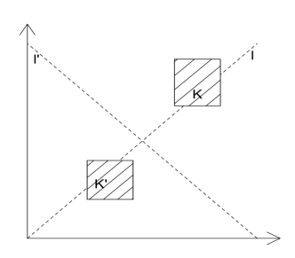
Figure 1: Location of rectangles $K$ and $K^{\prime}$.

The limit random field $\{V(x,y)\}$ in (5.12) is assumed to have dependent increments, in the following sense. Given a continuous-time random field $V=\{V(x,y)\}$, the increment of $V$ on rectangle $K=K_{(u,v),(x,y)}=\{(z,w)\in\mathbb{R}^{2}:u<z\leq x,u<w\leq y\}$ (with sides parallel to the coordinate axes) is defined as the (double) difference:

$$V(K):=V(x,y)-V(u,y)-V(x,v)+V(u,v).$$

If $\ell=\{(x,y)\in R^{2}:ax+by=c\}\subset\mathbb{R}^{2}$ is a line, we say that rectangles $K$ and $K^{\prime}$ are separated by $\ell$ if they lie on different sides of $\ell$. Given a line $\ell=\{(x,y)\in\mathbb{R}^{2}:ax+by=0\}$, we say that $V$ has independent increments in direction $\ell$ if for any orthogonal line $\ell^{\prime}=\{(x,y)\in\mathbb{R}^{2}:a^{\prime}x+b^{\prime}y=c^{\prime}\},\ell^{\prime}\bot\ell$ and any two rectangles $K,K^{\prime}$ separated by $\ell^{\prime}$, increments $V(K)$ and $V(K^{\prime})$ are independent r.v.’s; else $V$ has dependent increments in direction $\ell$ (see Fig. 1). Finally, we say that a random field $V$ has dependent increments if $V$ has dependent increments in each direction. The above definition of anisotropic distributional long memory is contrasted in [2013] with that of isotropic distributional long memory, with the only difference that in the latter case, (5.12) is supposed to hold with $H_{1}=H_{2}$, in other words, the rectangles $K_{[nx,ny]}$ grow proportionally in each direction. In both cases, the limit random field satisfies the scaling relation

$$\{\lambda V(x,y)\}\ \stackrel{{\scriptstyle\rm fdd}}{{=}}\ \{V(\lambda^{1/H_{1}}x,\lambda^{1/H_{2}}y)\},\qquad\forall\,\lambda>0.$$ (5.13)

(5.13) is a particular case of operator scaling random field (osrf) introduced in [2007]; for $H_{1}=H_{2}$ (5.13) agrees with self-similar random field (ssrf). [2013] show that the aggregated 2N and 3N $\alpha-$stable random fields $\{\mathfrak{X}_{2}(t,s)\}$ and $\{\mathfrak{X}_{3}(t,s)\}$ satisfy the above definition of anisotropic long memory with $H_{1}=\frac{(1/2)+\alpha-\beta}{\alpha},H_{2}=2H_{1}$ for any $1<\alpha\leq 2,0<\beta<\alpha-1$, and identify the limiting osrf’s $V_{2}$ and $V_{3}$ as stochastic integrals with respect to an $\alpha-$stable random measure with integrands involving the limiting Green functions $h_{2}$ and $h_{3}$. On the other hand, the 4N field $\{\mathfrak{X}_{4}(t,s)\}$ is proved to satisfy the isotropic long memory property with $H_{1}=H_{2}=2(\alpha-\beta)/\alpha$ and a limiting field $V_{4}$ involving the limit Green function $h_{4}(t,s,z)=\lim_{\lambda\to\infty}g_{4}([\lambda t],[\lambda s],1-z/\lambda^{2})$. The Green functions $h_{i},i=2,3,4$ have a classical form of potentials of one-dimensional heat equation and the Helmholtz equation in $\mathbb{R}^{2}$ (see [2013]).

6 Disaggregation

Aggregation by itself inflicts a considerable loss of information about the evolution of individual “micro-agents”, the latter being largely determined by the mixing distribution. The disaggregation problem is to recover the “lost information”, or the mixing distribution from the spectral density or other characteristics of the aggregated series. As a first step in this direction we need to identify the class of spectral densities which arise from aggregation of short memory (SM) processes with random parameters. [2006], [2001] obtained an analytic characterization of the class of spectral densities which can be written as mixtures of infinitely differentiable SM spectral densities. Further results in this direction were obtained in [2007]. For example, the well-known FARIMA(0,$d$,0) spectral density $f(y)=(2\pi)^{-1}|2\sin(|y|/2)|^{-2d}$ can be written as the mixture $f(y)=\int_{0}^{1}\phi(x)|1-x{\rm e}^{{\rm i}y}|^{-2}\phi(x){\rm{d}}x$ of the AR(1) processes corresponding to the mixing density

$$\phi(x)\ =\ C(d)x^{d-1}(1-x)^{1-2d}(1+x).$$

See [2007] for this and some other examples.

The above disaggregation problem naturally leads to statistical problems such as estimation of the mixing distribution from observed data. The observations may come either from the (limit) aggregated process, or from observed individual processes (sometimes also called panel data). Below we review several methods of estimation of $\phi$ in the autoregressive aggregation scheme described in Sec. 1. Note that (1.6) means that the covariances of the limit aggregated process are nothing else but the moments of the finite measure having density $(1-x^{2})^{-1}\phi(x)$. In fact, being supported by $[0,1)$, this measure is uniquely determined by its moments, so that the statistical problem of recovering the mixture density from observations $\mathfrak{X}(1),\dots,\mathfrak{X}(n)$ with finite variance is relevant. The last problem is much harder and is still open for the infinite variance aggregated process $\{\mathfrak{X}(t)\}$ defined in (2.4) (Sec.  2).

Estimation from panel data. Consider a panel of $N$ independent AR(1) processes, each of length $n$. [1978] and [2010] give estimates of $\phi$ under the assumption that $\phi$ belongs to some parametric family. The main example is the family of Beta-type distribution of the form

$$\phi_{p,q}(x)\ =\ \frac{2}{B(p,q)}\,x^{2p-1}(1-x^{2})^{q-1},\quad x\in[0,1),\ p>1,q>1.$$ (6.1)

In this context the estimation of $\phi$ is reduced to the estimation of parameter $(p,q)$. We outline briefly the two approaches.

[1978] suggested to use the classical method of moments using the following relation between the moments of $\phi$ and the auto-covariances $\gamma(k)=\mathrm{E}X_{j}(0)X_{j}(k)$ (1.3) of individual AR(1) processes,

$$\mu_{k}\ =\ \int_{0}^{1}x^{k}\phi(x){\rm{d}}x\ =\ \frac{\gamma(k)-\gamma(k+2)}{\gamma(0)-\gamma(2)}.$$ (6.2)

From panel data, the $\gamma(k)$’s can be estimated as

$$\frac{1}{(n-k+1)N}\sum_{t=1}^{n-k}\sum_{j=1}^{N}X_{j}(t)X_{j}(t+k).$$

[1978] proved the asymptotic normality of the corresponding estimates of moments $\mu_{k},0\leq k\leq n$ when $N$ goes to infinity and $n$ is fixed.

[2010] proposed an alternative method based on the maximum likelihood estimate (MLE) calculated from estimated observations. The unobserved coefficients $a_{i}$ of autoregressive processes $\{X_{i}(t)\}$, $i=1,\dots,N$, are estimated by a truncated version of lag-one autocorrelation

$$\widehat{a}_{i,n,h}\ =\ \min\{\max\{\widehat{a}_{i,n},h\},1-h\}\ \ {\text{with}}\ \ \widehat{a}_{i,n}\ =\ \frac{\sum_{t=1}^{n}X_{i}(t)X_{i}(t-1)}{\sum_{t=1}^{n}X_{i}^{2}(t)},\quad h>0.$$

In this way we obtain $N$ ”pseudo” observations $\widehat{a}_{1,n,h}$, $\widehat{a}_{2,n,h}$, …, $\widehat{a}_{N,n,h}$ of r.v. $a$. Then, the parameters $p$ and $q$ in (6.1) are estimated by maximizing the likelihood, viz. $(\hat{p},\hat{q})=\arg\max_{p,q}\prod_{i=1}^{N}\phi_{p,q}(\widehat{a}_{i,n,h})$. [2010] proved the convergence in probability of the above MLE estimate and its asymptotic normality with the convergence rate $\sqrt{N}$ under the following conditions on the sample sizes and the truncation parameter $h$: $n,N\to\infty$, $h\to 0$, $(\log h)^{2}/\sqrt{N}\to 0$, $\sqrt{N}h^{\min(p,q)}\to 0$ and $\sqrt{N}h^{-2}n^{-1}\to 0$.

Estimation from the limit aggregated process. Assume that a sample $\mathfrak{X}(1),\dots,\mathfrak{X}(n)$ of size $n$ is observed from the limited aggregated process. Under a parametric assumption about $\phi$, the estimator proposed by [1978] can be easily adapted to this context, because the limit aggregated process and the individual AR(1) have the same covariances.

[2006], [2010] use the relation (6.2) to construct a non-parametric estimate of $\phi$ under the assumption that

$$\phi(x)\ =\ (1-x)^{\beta_{1}}(1+x)^{\beta_{2}}\psi(x),\qquad\beta_{1}>0,\ \beta_{2}>0,$$ (6.3)

where $\psi(a)$ is continuous on $[-1,1]$ and does not vanishes at $+1$, $-1$, implying $\mathrm{E}(1-a^{2})^{-1}<\infty$. The above-mentioned nonparametric estimator is based on the expansion of the mixing density in the orthonormal basis of Gegenbauer’s polynomials in the space $L^{2}(w^{(\alpha)})$ with weight function $w^{(\alpha)}(x)=(1-x^{2})^{\alpha}$ and $\alpha>-1$. The estimate is defined as

$$\widehat{\phi}_{n}(x)\ :=\ (1-x^{2})^{\alpha}\frac{1}{\sigma^{2}}\sum_{k=0}^{K_{n}}\widehat{\zeta}_{n,k}G_{k}^{(\alpha)}(x),$$ (6.4)

where the coefficients $\widehat{\zeta}_{n,k}$ are defined as follows

$$\widehat{\zeta}_{n,k}\ :=\ \sum_{j=0}^{k}g_{k,j}^{(\alpha)}(\widehat{\gamma}_{n}(j)-\widehat{\gamma}_{n}(j+2)),$$ (6.5)

with $\widehat{\gamma}_{n}(j)$ the sample covariance of the zero mean aggregated process $\{\mathfrak{X}(t),\,t=1,\dots,n\}$.

The choice of $(K_{n})$ is crucial to obtain consistent estimate of $\phi$. Under the condition $\int\frac{\phi(x)^{2}}{(1-x^{2})^{\alpha}}{\rm{d}}x<\infty,$ [2006] showed that if $K_{n}$ is a nondecreasing sequence which tends to infinity at rate $[\gamma\log(n)]$, $0<\gamma<(2\log(1+\sqrt{2}))^{-1}$ then

$$\int_{-1}^{1}\frac{\mathrm{E}(\widehat{\phi}_{n}(x)-\phi(x))^{2}}{(1-x^{2})^{\alpha}}{\,\mathrm{d}}x\ \to\ 0.$$

[2010] proved the asymptotic normality $\frac{\widehat{\phi}_{n}(x)-\mathrm{E}\widehat{\phi}_{n}(x)}{\sqrt{\operatorname{Var}(\widehat{\phi}_{n}(x))}}\rightarrow_{\rm d}N(0,1),$ for every fixed $x\in(-1,1)$. The estimate (6.4) depends on the variance $\sigma^{2}=\gamma(0)-\gamma(2)$ which can be replaced by its estimate $\widehat{\sigma}^{2}=\widehat{\gamma}_{n}(0)-\widehat{\gamma}_{n}(2).$ [2013] proved that the modified estimate is still consistent in a weaker sense, since

$$\int_{-1}^{1}\frac{(\widehat{\phi}_{n}(x)-\phi(x))^{2}}{(1-x^{2})^{\alpha}}{\,\mathrm{d}}x\ \stackrel{{\scriptstyle\rm P}}{{\rightarrow}}\ 0.$$

The estimate in (6.4) has been extended non-gaussian aggregated process in (3.4) with finite variance discussed in Sec. 3 (see [2013]) and to some aggregated random field models (see [2013]).

It should be noted that the estimate (6.4) is not adapted to the limit aggregated process with common innovations. For such models, [2006] proposed a parametric estimate of $\phi$, assuming that $\phi$ is a polynomial. The last condition, however, excludes the case of long memory processes.

References

- Astrauskas (1983) Astrauskas, A. (?). Limit theorems for sums of linearly generated random variables. Lithuanian Mathematical Journal, 23, 127–134.
- 2009 Azomahou, T.T. (?). Memory properties and aggregation of spatial autoregressive models. Journal of Statistical Planning and Inference, 139, 2581–2579.
- 1996 Baillie, R. T. (?). Long memory processes and fractional integration in econometrics. Journal of Econometrics, 73, 5–59.
- 2001 Barndorff-Nielsen, O. E. (?). Superposition of Ornstein–Uhlenbeck type processes. Theory of Probability and Its Applications, 45, 175–194.
- 2013 Beran, Feng-Y. Ghosh S. J. and Kulik, R. (?). Long-memory processes: Probabilistic properties and statistical methods. Springer.
- 2010 Beran, J., Schützner, M. and Ghosh, S. (?). From short to long memory: Aggregation and estimation. Computational Statistics and Data Analysis, 54, 2432–2442.
- 2007 Biermé, H., Meerschaert, M. M. and Scheffler, H. P. (?). Operator scaling stable random fields. Stochastic Processes and Applications, 117, 312–332.
- 2007 Celov, D., Leipus, R. and Philippe, A. (?). Time series aggregation, disaggregation and long memory. Lithuanian Mathematical Journal, 47, 379–393.
- 2010 Celov, D., Leipus, R. and Philippe, A. (?). Asymptotic normality of the mixture density estimator in a disaggregation scheme. Journal of Nonparametric Statistics, 22, 425–442.
- 2006 Chong, T. T. (?). The polynomial aggregated AR(1) model. Econometrics Journal, 9, 98–122.
- 1984 Cox, D. R. (?). Long-range dependence: A review. In Statistics: An Appraisal (eds H. A. David and H. T. David), pp. 55–74. Iowa State Univ. Press, Iowa.
- 2006 Dacunha-Castelle, D. and Fermin, L. (?). Disaggregation of long memory processes on class. Electronic Communications in Probability, 11, 35–44.
- 2001 Dacunha-Castelle, D. and Oppenheim, G. (?). Mixtures, aggregation and long-memory. Prepublications, Université de Paris-Sud Mathématiques.
- 1996 Ding, Z. and Granger, C. W. J. (?). Modeling volatility persistence of speculative returns: a new approach. Journal of Econometrics, 73, 185–215.
- 2011 Dombry, C. and Kaj, I. (?). The on-off network traffic model under intermediate scaling. Queueing Systems, 69, 29–44.
- 2006 Gaigalas, R. (?). A Poisson bridge between fractional Brownian motion and stable Lévy motion. Stochastic Processes and Applications, 116, 447–462.
- 2003 Gaigalas, R. and Kaj, I. (?). Convergence of scaled renewal processes and a packet arrival model. Bernoulli, 9, 671–703.
- 2012 Giraitis, L., Koul, H. L. and Surgailis, D. (?). Large Sample Inference for Long Memory Processes. Imperial College Press, London.
- 2010 Giraitis, L., Leipus, R. and Surgailis, D. (?). Aggregation of random coefficient GLARCH(1,1) process. Econometric Theory, 26, 406–425.
- 1988 Gonçalves, E. and Gouriéroux, C. (?). Aggrégation de processus autoregressifs d’ordre 1. Annales d’Economie et de Statistique, 12, 127–149.
- 1980 Granger, C. W. J. (?). Long memory relationship and the aggregation of dynamic models. Journal of Econometrics, 14, 227–238.
- 1997 Heyde, C. C. and Yang, Y. (?). On defining long-range dependence. Journal of Applied Probability, 34, 939–944.
- 2011 Jirak, M. (?). Asymptotic behavior of weakly dependent aggregated processes. Periodica Mathematica Hungarica, 62, 39–60.
- 2004 Kazakevičius, V., Leipus, R. and Viano, M.-C. (?). Stability of random coefficient ARCH models and aggregation schemes. Journal of Econometrics, 120, 139–158.
- 1962 Lamperti, J. (?). Semi-stable stochastic processes. Transactions of American Mathematical Society, 104, 62–78.
- 2007 Lavancier, F. (?). Invariance principles for non-isotropic long memory random fields. Statistical Inference for Stochastic Processes, 10, 255–282.
- 2011 Lavancier, F. (?). Aggregation of isotropic random fields. Journal of Statistical Planning and Inference, 141, 3862–3866.
- 2013 Lavancier, F., Leipus, R. and Surgailis, D. (?). Aggregation of anisotropic random-coefficient autoregressive random field. Preprint.
- 2006 Leipus, R., Oppenheim, G., Philippe, A. and Viano, M.-C. (?). Orthogonal series density estimation in a disaggregation scheme. Journal of Statistical Planning and Inference, 136, 2547–2571.
- 2005 Leipus, R., Paulauskas, V. and Surgailis, D. (?). Renewal regime switching and stable limit laws. Journal of Econometrics, 129, 299–327.
- 2003 Leipus, R. and Surgailis, D. (?). Random coefficient autoregression, regime switching and long memory. Advances in Applied Probability, 35, 1–18.
- 2002 Leipus, R. and Viano, M.-C. (?). Aggregation in ARCH models. Lithuanian Mathematical Journal, 42, 54–70.
- 2013 Leonenko, N. and Taufer, E. (?). Disaggregation of spatial autoregressive processes. Spatial Statistics, 3, 1–20.
- 1998 Lobato, I. N. and Savin, N. E. (?). Real and spurious long-memory properties of stock-market data (with comments). Journal of Business & Economic Statistics, 16, 261–283.
- 2003 Mikosch, T. (?). Modeling dependence and tails for financial time series. In Extreme Values in Finance, Telecommunications and the Environment (eds B. Finkenstädt and H. Rootzén), pp. 185–286. Chapman & Hall.
- 2002 Mikosch, T., Resnick, S., Rootzén, H. and Stegeman, A. (?). Is network traffic approximated by stable Lévy motion or fractional Brownian motion? Annals of Applied Probability, 12, 23–68.
- 2000 Mikosch, T. and Samorodnitsky, G. (?). Ruin probability with claims modeled by a stationary ergodic stable process. Annals of Probability, 28, 1814–1851.
- 2004 Oppenheim, G. and Viano, M.-C. (?). Aggregation of random parameters Ornstein-Uhlenbeck or AR processes: some convergence results. Journal of Time Series Analysis, 25, 335–350.
- 2013 Paulauskas, V. (?). On –covariance, long, short and negative memories for sequences of random variables with infinite variance. Preprint.
- 2013 Perilioğlu, K. and Puplinskaitė, D. (?). Asymptotics of the ruin probability with claims modeled by -stable aggregated AR(1) process. Turkish Journal of Mathematics, 37, 129–138.
- 2013 Philippe, A., Puplinskaitė, D. and Surgailis, D. (?). Contemporaneous aggregation of a triangular of random coefficient AR(1) processes. Preprint.
- 2013 Pilipauskaitė, V. and Surgailis, D. (?). Large-scale temporal and contemporaneous aggregation of random-coefficient ar(1) processes. Preprint.
- 2004 Pipiras, V., Taqqu, M. S. and Levy, L. B. (?). Slow, fast, and arbitrary growth conditions for renewal-reward processes when both the renewals and the rewards are heavy-tailed. Bernoulli, 10, 121–163.
- 2009 Puplinskaitė, D. and Surgailis, D. (?). Aggregation of random coefficient AR(1) process with infinite variance and common innovations. Lithuanian Mathematical Journal, 49, 446–463.
- 2010 Puplinskaitė, D. and Surgailis, D. (?). Aggregation of random coefficient AR(1) process with infinite variance and idiosyncratic innovations. Advances in Applied Probability, 42, 509–527.
- 2013 Puplinskaitė, D. and Surgailis, D. (?). Agggregation of autoregressive random fields and anisotropic long memory. Preprint.
- 1989 Rajput, B. S. and Rosinski, J. (?). Spectral representations of infinitely divisible processes. Probability Theory and Related Fields, 82, 451–487.
- 1978 Robinson, P. (?). Statistical inference for a random coefficient autoregressive model. Scand. J. Statist., 5, 163–168.
- 1994 Samorodnitsky, G. and Taqqu, M. S. (?). Stable Non-Gaussian Random Processes. Chapman & Hall, New York.
- 1999 Sato, K.-I. (?). Lévy Processes and Infinitely Divisible Distributions. Cambridge University Press, Cambridge.
- 1993 Surgailis, D., Rosinski, J., Mandrekar, V. and Cambanis, S. (?). Stable mixed moving averages. Probability Theory and Related Fields, 97, 543–558.
- 2007 Teyssière, G. and Kirman, A. P. (?) (eds). Long Memory in Economics. Springer, Berlin, Heidelberg.
- 2007 Ward, L. M. and Greenwood, P. E. (?). noise. Scholarpedia, 2(12), 1537.
- 1997 Willinger, W., Taqqu, M. S., Sherman, R. and Wilson, D. V. (?). Self-similarity through high-variability: statistical analysis of Ethernet LAN traffic at the source level. IEEE/ACM Transactions on Networking, 5, 71–86.
- 2004 Zaffaroni, P. (?). Contemporaneous aggregation of linear dynamic models in large economies. Journal of Econometrics, 120, 75–102.
- 2007a Zaffaroni, P. (?). Aggregation and memory of models of changing volatility. Journal of Econometrics, 136, 237–249.
- 2007b Zaffaroni, P. (?). Contemporaneous aggregation of GARCH processes. Journal of Time Series Analysis, 28, 521–544.