Third-Order Edge Statistics: Contour Continuation, Curvature, and Cortical Connections

Abstract

Association field models have attempted to explain human contour grouping performance, and to explain the mean frequency of long-range horizontal connections across cortical columns in V1. However, association fields only depend on the pairwise statistics of edges in natural scenes. We develop a spectral test of the sufficiency of pairwise statistics and show there is significant higher order structure. An analysis using a probabilistic spectral embedding reveals curvature-dependent components.

1 Introduction

Natural scene statistics have been used to explain a variety of neural structures. Driven by the hypothesis that early layers of visual processing seek an efficient representation of natural scene structure, decorrelating or reducing statistical dependencies between subunits provides insight into retinal ganglion cells [16], cortical simple cells [13, 2], and the firing patterns of larger ensembles [17]. In contrast to these statistical models, the role of neural circuits can be characterized functionally [3, 14] by positing roles such as denoising, structure enhancement, and geometric computations. Such models are based on evidence of excitatory connections among co-linear and co-circular neurons [5], as well as the presence of co-linearity and co-circularity of edges in natural images [8], [7]. The fact that statistical relationships have a geometric structure is not surprising: To the extent that the natural world consists largely of piecewise smooth objects, the boundaries of those objects should consist of piecewise smooth curves.

Common patterns between excitatory neural connections, co-occurrence statistics, and the geometry of smooth surfaces suggests that the functional and statistical approaches can be linked. Statistical questions about edge distributions in natural images have differential geometric analogues, such as the distribution of intrinsic derivatives in natural objects. From this perspective, previous studies of natural image statistics have primarily examined “second-order” differential properties of curves; i.e., the average change in orientation along curve segments in natural scenes. The pairwise statistics suggest that curves tend toward co-linearity, in that the (average) change in orientation is small. Similarly, for long-range horizontal connections, cells with similar orientation preference tend to be connected to each other.

Is this all there is? From a geometric perspective, do curves in natural scenes exhibit continuity in curvatures, or just in orientation? Are edge statistics well characterized at second-order? Does the same hold for textures?

To answer these questions one needs to examine higher-order statistics of natural scenes, but this is extremely difficult computationally. One possibility is to design specialized patterns, such as intensity textures [15], but it is difficult to generalize such results into visual cortex. We make use of natural invariances in image statistics to develop a novel spectral technique based on preserving a probabilistic distance. This distance characterizes what is beyond association field models (discussed next) to reveal the “third-oder” structure in edge distributions. It has different implications for contours and textures and, more generally, for learning.

2 Edge Co-occurrence Statistics

Edge co-occurrence probabilities are well studied [1, 8, 6, 11]. Following them, we use random variables indicating edges at given locations and orientations. More precisely, an edge at position, orientation $(x_{i},y_{i},\theta_{i})$, denoted $E_{i}$, is a $\{0,1\}$ valued random variable. Co-occurrence statistics examine various aspects of pairwise marginal distributions, which we denote by $P(E_{i},E_{j})$.

The image formation process endows scene statistics with a natural translation invariance. If the camera were allowed to rotate randomly about the focal axis, natural scene statistics would also have a rotational invariance. For computational convenience, we enforce this rotational invariance by randomly rotating our images. Thus,

$$P(E_{(x_{i},y_{i},\theta_{i})},...,E_{(x_{j},y_{j},\theta_{j})})=P(E_{(x_{i}+\delta x,y_{i}+\delta y,\theta_{i}+\delta\theta)},...,E_{(x_{j}+\delta x,y_{j}+\delta y,\theta_{j}+\delta\theta)})$$

We can then estimate joint distributions of nearby edges by looking at patches of edges centered at a (position, orientation) location $(x_{i},y_{i},\theta_{i})$ and rotating the patch into a canonical orientation and position that we denote $E_{0}=E_{(x_{0},y_{0},\theta_{0})}$.

$$P(E_{(x_{i},y_{i},\theta_{i})},...,E_{(x_{j},y_{j},\theta_{j})})=P(E_{(x_{i}-x_{j},y_{i}-y_{j},\theta_{i}-\theta_{j})},...,E_{(x_{0},y_{0},\theta_{0})})$$

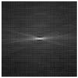
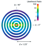
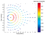
August and Zucker, 2000	Geisler et al, 2001	Elder & Goldberg, 2002

Figure 1: Association fields derive from image co-occurrence statistics. We interpret them as illustrating the probability (likelihood) of an edge near a horizontal edge at the center position.

Several examples of statistics derived from the distribution of $P(E_{i},E_{0})$ are shown in Fig. 1. These are pairwise statistics of oriented edges in natural images. The most important visible feature of these pairwise statistics is that of good continuation: Conditioned on the presence of an edge at the center, edges of similar orientation and horizontally aligned with the edge at the center have high probability. Note that all of the above implicitly or explicit enforced rotation invariance, either by only examining relative orientation with respect to a reference orientation or by explicit rotation of the images.

It is critical to estimate the degree to which these pairwise statistics characterize the full joint distribution of edges (Fig. 2). Many models for neural firing patterns imply relatively low order joint statistics. For example, spin-glass models imply pairwise statistics are sufficient, while Markov random fields have an order determined by the size of neighborhood cliques.

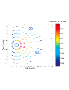
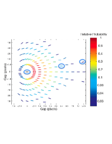
Figure 2: Two approximately equally likely triples of edges under the pairwise independence assumption of Elder et. al. Conditional independence is one of several possible pairwise distributional assumptions. Intuitively, however, the second triple is much more likely. We examine third-order statistics to demonstrate that this is in fact the case.

3 Contingency Table Analysis

To test whether the joint distribution of edges can be well described by pairwise statistics, we performed a contingency table analysis of edge triples at two different threshold levels. We computed estimated joint distributions for each triple of edges in an $11\times 11\times 8$ patch, not constructed to have an edge at the center. Using a $\chi^{2}$ test, we computed the probability that each edge triple distribution could occur under hypothesis $H_{0}:\{\text{No three way interaction}\}$. This is a test of the hypothesis that

$$\log P(E_{i},E_{j},E_{k})=f(E_{i},E_{j})+g(E_{j},E_{k})+h(E_{i},E_{k})$$

for each triple $(E_{i},E_{j},E_{k})$, and includes the cases of independent edges, conditionally independent edges, and other pairwise interactions. For almost all triples, this probability was extremely small. (The few edge triples for which the null hypothesis cannot be rejected consisted of edges that were spaced very far apart, which are far more likely to be nearly statistically independent of one another.)

$n=150705016$	threshold $=.05$	threshold $=.1$
percentage of triples where $p_{H_{0}}>$ .05	0.0082%	0.0067%

4 Counting Triple Probabilities

We chose a random sampling of black and white images from the van Hataren image dataset[10]. They were randomly rotated and then filtered using oriented Gabor filters covering 8 angles from $[0,\pi)$. Each Gabor has a carrier period of 1.5 pixels per radian and an envelope standard deviation of 5 pixels. The filters were convolved in near quadrature pairs, squared and summed. To restrict analysis to the statistics of curves, we applied local non-maxima suppression across orientation columns in a direction normal to the given orientation. This removes effects of filter blurring and oriented texture patterns (considered shortly). The resulting edge maps were subsampled to eliminate statistical dependence due to overlapping filters.

Thresholding the edge map yields $E:U\rightarrow\{0,1\}$, where $U\subset\mathbb{R}^{2}\times\mathbb{S}$ is a discretization of $\mathbb{R}^{2}\times\mathbb{S}$. We treat $E$ as a function or a binary vector as convenient. We randomly select $21\times 21\times 8$ image patches with an oriented edge at the center, and denote these characteristic patches by $V_{i}$

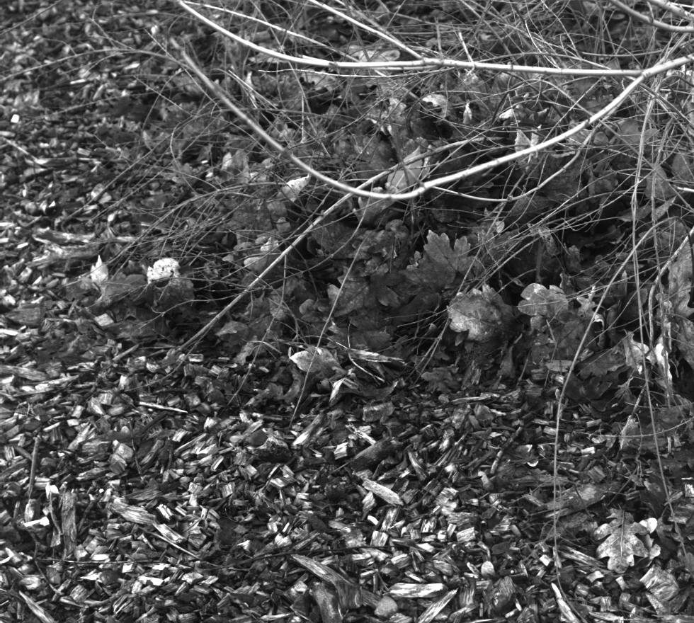
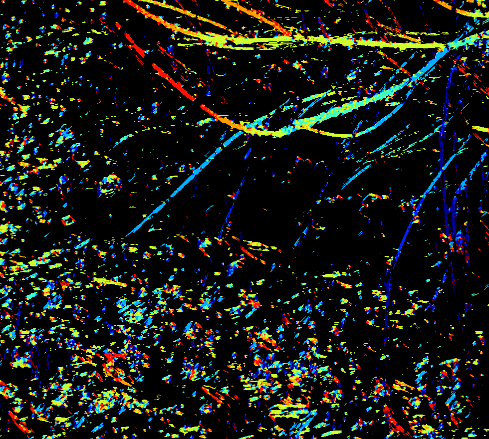
(a)	(b)

Figure 3: Example image (a) and edges (b) for statistical analysis. Note: color corresponds to orientation

Since edges are significantly less frequent than their absence, we focus on (positive) edge co-occurance statistics. For simplicity, we denote $P(E_{i}=1,E_{j}=1,E_{k}=1)$ by $P(i,j,k)$ (A small orientation anisotropy has been reported in natural scenes (e.g., [9]), but does not appear in our data because we effectively averaged over orientations by randomly rotating the images.)

We compute the matrix $P(i,j|0)$ where

$$P(i,j|0) =P(E_{i}=1,E_{j}=1|E_{0}=1)$$

$$\sim\frac{1}{n}\sum_{i=1}^{n}V_{i}V_{i}^{T}$$

where $V_{i}$ is a (vectorized) random patch of edges centered around an edge with orientation $\theta_{i}=0$.

5 Visualizing Triples of Edges

By analogy with the pairwise analysis above, we seek to find those edge triples that frequently co-occur. But this is significantly more challenging. For pairwise statistics, one simply fixes an edge to lie in the center and “colors” the other edge by the joint probability of the co-occurring pair (Fig. 1). No such plot exists for triples of edges. Even after conditioning, there are over 12 million edge triples to consider.

Our trick: Embed edges in a low dimensional space such that the distance between the edges represents the relative likelihood of co-occurrence. We shall do this in a manner such that distance in Embedded Space $\sim$ Relative Probability.

As before, let $E_{i}$ be a binary random variable, where $E_{i}=1$ means there is an edge at location $v_{i}=(x_{i},y_{i},\theta_{i})$. We define a distance between edges

$$D^{2}_{+}(v_{i},v_{j})=P(i,i|0)-2P(i,j|0)+P(j,j|0)$$

The first and the last terms represent pairwise co-occurrence probabilities; i.e., these are the association field. The middle term represents the interaction between $E_{i}$ and $E_{j}$ conditioned on the presence of $E_{0}$. Thus this distance is zero if the edges always co-occur in images, given the horizontal edge at the origin, and is large if the pair of edges frequently occur with the horizontal edge but rarely together. (The relevance to learning is discussed below.)

We will now show how, for natural images, edges can be placed in a low dimensional space where the distance in that space will be proportional to this probabilistic distance.

6 Dimensionality Reduction via Spectral Theorem

Exploiting the fact that $P(i,j|0)$ is a positive semi-definite matrix, we introduce the spectral expansion

$$P(i,j|0)=\sum_{l=1}^{n}\lambda_{l}\phi_{l}(i)\phi_{l}(j)$$

where $\phi_{l}$ is an eigenvector of the $K$ matrix.

Define the spectral embedding $\Phi:\left(\begin{array}[]{c}x_{i}\\ y_{i}\\ \theta_{i}\end{array}\right)\rightarrow\mathbb{R}^{n}$

$$\Phi(v_{i})=\{\sqrt{\lambda_{1}}\phi_{1}(i),\sqrt{\lambda_{2}}\phi_{2}(i),...,\sqrt{\lambda_{n}}\phi_{n}(i)\}$$ (1)

The Euclidean distance between embedded points is then

$$\|\Phi(v_{i})-\Phi(v_{j})\|^{2} =\langle\Phi(v_{i}),\Phi(v_{i})\rangle-2\langle\Phi(v_{i}),\Phi(v_{j})\rangle+\langle\Phi(v_{j}),\Phi(v_{j})\rangle$$

$$=P_{+}(i,i|0)-2P_{+}(i,j|0)+P_{+}(j,j|0)$$

$$=D^{2}_{+}(v_{i},v_{j})$$

$\Phi$ maps edges to points in an embedded space where squared distance is equal to relative probability; we refer to this as diffusion distance.

The usefulness of this embedding comes from the fact that the spectrum of $P(i,j,0)$ decays rapidly (Fig. 4). Therefore we truncate $\Phi$, including only dimensions with high eigenvalues. This gives a dramatic reduction in dimensionality, and allows us to visualize the relationship between triples of edges (Fig. 4).

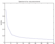
Figure 4: Spectrum of $P(i,j|0)$. Other spectra are similar. Note rapid decay of the spectrum indicating the diffusion distance is well captured by embedding using only the first few eigenfunctions.

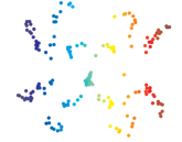
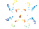
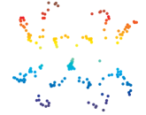
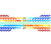
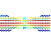
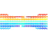
$\phi_{2}$	$\phi_{3}$	$\phi_{4}$

Figure 5: Display of third-order edge structure showing how oriented edges are related to their spectral embeddings. (top) Spectral embeddings. Note clusters of co-occuring edges. (bottom) Edge distributions. The eigenvectors of $P(i,j,0)$ are used to color both the edges and the embedding. Clusters of edges in this embedding have a high probability of co-occurring along with the edge in the center. Compare with Fig. 1 where red edges all have high probability of occurring with the center, but no information is known about their co-occurrence probability.

To highlight information not contained in the association field, we normalized our probability matrix by its row sums, and removed all low-probability edges. Embedding the mapping from $\mathbb{R}^{2}\times\mathbb{S}\rightarrow\mathbb{R}^{m}$ reveals the cocircular structure of edge triples in the image data (Fig. 5. The colors along each column correspond, so similar colors map to nearby points along the dimension corresponding to the row. Under this dimensionality reduction, each small cluster in diffusion space corresponds to half of a cocircular field. In effect, the coloring by $\phi_{2}$ shows good continuation in orientation (with our crude quantization) while the coloring by $\phi_{4}$ shows co-circular connections. In effect, then, the association field is the union of co-circular connections, which also follows from marginalizing the third-order structure away. We used 40,000 ($21\times 21\times 8$) patches.

7 Implications: “Cells that fire together wire together”

Shown above are low dimensional projections of the diffusion map and their corresponding colorings in $\mathbb{R}^{2}\times\mathbb{S}$. To provide a neural interpretation of these results, let each point in $\mathbb{R}^{2}\times\mathbb{S}$ represent a neuron with a receptive field centered at the point $(x,y)$ with preferred orientation $\theta$. Each cluster then signifies those neurons that have a high probability of co-firing given that the central neuron fires, so clusters in diffusion coordinates should be “wired” together by the Hebbian postulate. Such curvature-based facilitation can explain the non-monotonic variance in excitatory long-range horizontal connections in V1 [3, 4]. It may also have implications for the receptive fields of V2 neurons. As clusters of co-circular V1 complex cells are correlated in their firing, it may be efficient to represent them with a single cell with excitatory feedforward connections. This predicts that efficient coding models that take high order interactions into account should exhibit cells tuned to curved boundaries.

Our approach also has implications beyond excitatory connections for boundary facilitation. We repeated our conditional spectral embedding, but now conditioned on the absence of an edge at the center (Fig. 6). This could provide a model for inhibition, as clusters of edges in this embedding are likely to co-occur conditioned on the absence of an edge at the center. We find that the embedding is only one dimensional, with the significant eigenvector a monotonic function of orientation difference from the center orientation. Compared to excitatory connections, this suggests that inhibition is relatively unstructured, and agrees with many neurobiological studies.

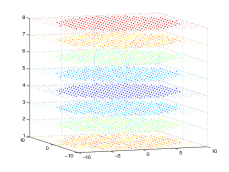
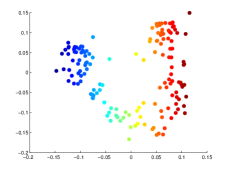
Figure 6: Embeddings conditioned on the absence of an edge at the center location. Note how less structured it is, compared to the positive embeddings. As such it could serve as a model for inhibitory connections, which span many orientations.

Finally, we repeated this third-order analysis (but without local non-maxima supression) on a structured model for isotropic textures on 3D surfaces and again found a curvature dependency (Fig. 7). Every 3-D surface has a pair of associated dense texture flows in the image plane that correspond to the slant and tilt directions of the surface. For isotropic textures, the slant direction corresponds to the most likely orientation signalled by oriented filters. Hence, the distribution of these directions in 3-D shape are an excellent proxy for measuring the response of orientation filters to dense textured objects.

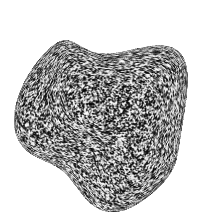
(a)	(b)

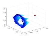
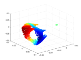
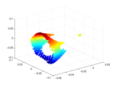
$\phi_{2}$	$\phi_{3}$	$\phi_{4}$

Figure 7: (top) Oriented textures provide information about surface shape. (bottom) As before, we looked at the conditional co-occurrence matrices of edge orientations over a series of randomly generated shapes. Slant orientations and embedding colored by each eigenvector. The edge map is thresholded to contain only orientations of high probability. The resulting embedding $\phi(v_{i})$ of those orientations is shown below. The eigenvectors of $P(i,j,0)$ are used to color both the orientations and the embedding. Clusters of orientations in this embedding have a high probability of co-occurring along with the edge in the center.

As this is a representation of a dense vector field, it is more difficult to interpret than the edge map. We therefore applied k-means clustering in the embedded space and segmented the resulting vector field. The resulting clusters show two-sided continuation of the texture flow with a fixed tangential curvature (Fig. 8).

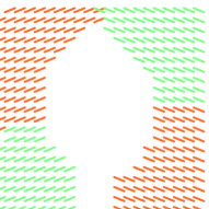
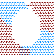
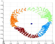
Figure 8: Clustering of dense texture flows. Color corresponds to the cluster index. Clusters were separated into different figures so as to minimize the $x,y$ overlap of the orientations. Embedding on the right is identical to the embeddings above, but viewed along the $\phi_{3},\phi_{4}$ axes.

In summary, then, we have developed a method for revealing third-order orientation structure by spectral methods. It is based on a diffusion metric that makes third-order terms explicit, and yields a Euclidean distance measure by which edges can be clustered. Given that long-range horizontal connections are consistent with these clusters, how biological learning algorithms converge to them remains an open question. Given that research in computational neuroscience is turning to third-order [12] and specialized interactions, this question now becomes more pressing.

References

- [1] Jonas August and Steven W Zucker. The curve indicator random field: Curve organization via edge correlation. In Perceptual organization for artificial vision systems, pages 265–288. Springer, 2000.
- [2] A.J. Bell and T.J. Sejnowski. The “independent components” of natural scenes are edge filters. Vision research, 37(23):3327–3338, 1997.
- [3] O. Ben-Shahar and S. Zucker. Geometrical computations explain projection patterns of long-range horizontal connections in visual cortex. Neural Computation, 16(3):445–476, 2004.
- [4] William H Bosking, Ying Zhang, Brett Schofield, and David Fitzpatrick. Orientation selectivity and the arrangement of horizontal connections in tree shrew striate cortex. The Journal of Neuroscience, 17(6):2112–2127, 1997.
- [5] Heather J. Chisum, François Mooser, and David Fitzpatrick. Emergent properties of layer 2/3 neurons reflect the collinear arrangement of horizontal connections in tree shrew visual cortex. The Journal of Neuroscience, 23(7):2947–2960, 2003.
- [6] James H Elder and Richard M Goldberg. Ecological statistics of gestalt laws for the perceptual organization of contours. Journal of Vision, 2(4), 2002.
- [7] J.H. Elder and RM Goldberg. The statistics of natural image contours. In Proceedings of the IEEE Workshop on Perceptual Organisation in Computer Vision. Citeseer, 1998.
- [8] WS Geisler, JS Perry, BJ Super, and DP Gallogly. Edge co-occurrence in natural images predicts contour grouping performance. Vision research, 41(6):711–724, 2001.
- [9] Bruce C Hansen and Edward A Essock. A horizontal bias in human visual processing of orientation and its correspondence to the structural components of natural scenes. Journal of Vision, 4(12), 2004.
- [10] J. H. van Hateren and A. van der Schaaf. Independent component filters of natural images compared with simple cells in primary visual cortex. Proceedings: Biological Sciences, 265(1394):359–366, Mar 1998.
- [11] Norbert Krüger. Collinearity and parallelism are statistically significant second-order relations of complex cell responses. Neural Processing Letters, 8(2):117–129, 1998.
- [12] Ifije E Ohiorhenuan and Jonathan D Victor. Information-geometric measure of 3-neuron firing patterns characterizes scale-dependence in cortical networks. Journal of computational neuroscience, 30(1):125–141, 2011.
- [13] Bruno A Olshausen et al. Emergence of simple-cell receptive field properties by learning a sparse code for natural images. Nature, 381(6583):607–609, 1996.
- [14] T.K. Sato, I. Nauhaus, and M. Carandini. Traveling waves in visual cortex. Neuron, 75(2):218–229, 2012.
- [15] Gašper Tkačik, Jason S Prentice, Jonathan D Victor, and Vijay Balasubramanian. Local statistics in natural scenes predict the saliency of synthetic textures. Proceedings of the National Academy of Sciences, 107(42):18149–18154, 2010.
- [16] JH Van Hateren. A theory of maximizing sensory information. Biological cybernetics, 68(1):23–29, 1992.
- [17] William E Vinje and Jack L Gallant. Sparse coding and decorrelation in primary visual cortex during natural vision. Science, 287(5456):1273–1276, 2000.