A Pseudo $su(1,1)$-Algebraic Deformation of the Cooper-Pair in the $su(2)$-Algebraic Many-Fermion Model

Abstract

A pseudo $su(1,1)$-algebra is formulated as a possible deformation of the Cooper-pair in the $su(2)$-algebraic many-fermion system. With the aid of this algebra, it is possible to describe behavior of individual fermions which are generated as the result of interaction with the external environment. The form presented in this paper is a generalization of a certain simple case developed recently by the present authors. Basic idea follows the $su(1,1)$-algebra in the Schwinger boson representation for treating energy transfer between the harmonic oscillator and the external environment. Hamiltonian is given under the idea of the phase space doubling in the thermo-field dynamics formalism and the time-dependent variational method is applied to this Hamiltonian. Its trial state is constructed in the frame deformed from the BCS-Bogoliubov approach to the superconductivity. Several numerical results are shown.

1 Introduction

It may be hardly necessary to mention, but the BCS-Bogoliubov approach to the superconductivity has made a central contribution to study of nuclear structure theory. The orthogonal set in this approach is determined through two steps. At first step, the state $|{\phi_{B}})$ given in the following plays the leading part:

$$|{\phi_{B}})=\frac{1}{\sqrt{\Gamma}}\exp\left(z{\widetilde{S}}_{+}\right)|{0})\ ,$$ (1.1a)

$$\Gamma=(1+|z|^{2})^{2\Omega_{0}}\ .$$ (1.1b)

Here, $\Gamma$, $z$, ${\widetilde{S}}_{+}$ and $|{0})$ denote normalization constant, complex parameter, the Cooper-pair creation and the fermion vacuum, respectively. Including ${\widetilde{S}}_{-}$ and ${\widetilde{S}}_{0}$, the set $({\widetilde{S}}_{\pm,0})$ forms the $su(2)$-algebra. Clearly, $|{\phi_{B}})$ is the state with zero seniority. But, it is not eigenstate of the fermion-number operator and plays a role of the quasiparticle vacuum. At second step, the states with nonzero seniority are constructed by operating the quasiparticles on $|{\phi_{B}})$ in appropriate manner. On the other hand, the Cooper-pair can be treated by the conventional technique of the $su(2)$-algebra. The orthogonal set in this approach is determined also through two steps. First is to construct the minimum weight state $|{m})$, which does not contain any Cooper-pair:

$${\widetilde{S}}_{-}|{m})=0\ .$$ (1.2)

Therefore, $|{m})$ is not necessary the state with zero seniority. Second is to construct the states orthogonal to $|{m})$ by operating ${\widetilde{S}}_{+}$ in appropriate manner. The above mention tells us that, for the two approaches, the orthogonal set is constructed in opposite orders. Therefore, without any argument, it may be not concluded that they are equivalent to each other.

In response to the above-mentioned situation, the present authors, recently, proposed a certain idea [1]. In this idea, the quasiparticle in the conservation of the fermion-number, which is called the “quasiparticle”, was introduced. Through the medium of this operator, it was shown that both are equivalent to each other in a certain sense. Further, in the paper following Ref.1, the present authors discussed another role of the “quasiparticle”: It leads to an idea of deformation of the Cooper-pair [2]. Hereafter, this paper will be referred to as (A). Any state $|{\phi})$ with zero seniority including $|{\phi_{B}})$ obeys the condition (A.13), which is strongly related to the “quasiparticle”. This condition does not lead to fix the form of $|{\phi})$ automatically and, then, new condition additional to the condition (A.13) is required. If the condition (A.17) is added, we obtain $|{\phi_{B}})$. In (A), we treated the case of the condition (A.18) in detail. In this case, $|{\phi})$ is obtained in the form

$$|{\phi})=\frac{1}{\sqrt{\Gamma}}\exp\left(z{\widetilde{\cal T}}_{+}\right)|{0})\ ,$$ (1.3a)

$$\Gamma=\sum_{n=0}^{2\Omega_{0}}(|z|^{2})^{n}\ .$$ (1.3b)

Here, ${\widetilde{\cal T}}_{+}$ is an operator factorized in the product of ${\widetilde{S}}_{+}$ and a certain operator. The definition of ${\widetilde{\cal T}}_{+}$ including ${\widetilde{\cal T}}_{-}$ and ${\widetilde{\cal T}}_{0}$ is given in the relation (A.36). The commutation relations among ${\widetilde{\cal T}}_{\pm,0}$, which are shown in the relation (A.39), suggest us that, in spite of considering of the $su(2)$-algebraic many-fermion model, the set $({\widetilde{\cal T}}_{\pm,0})$ resembles the $su(1,1)$-algebra in behavior. The form (1.3b) is given in the relation (A.25).

It is well known that, with the use of two kinds of boson operators, the $su(2)$- and the $su(1,1)$-algebra, the generators of which are denoted as ${\hat{S}}_{\pm,0}$ and ${\hat{T}}_{\pm,0}$, respectively, can be formulated. They are called the Schwinger boson representations [3]. For these two algebras, we prepare two boson-spaces: (1) the space constructed under a fixed magnitude of the $su(2)$-spin, $s(=0,1/2,1,\cdots,s_{\rm max})$ and (2) the space constructed under a fixed magnitude of the $su(1,1)$-spin, $t(=1/2,1,3/2,\cdots,\infty)$. Following the idea of the boson mapping [4], any operator in the space (1) can be mapped into the space (2). In the space (1), we can find the set $({\hat{\cal T}}_{\pm,0})$, which obeys

$${\hat{\cal T}}_{\pm,0}\ \stackrel{{\scriptstyle\textrm{(mapped)}}}{{\longrightarrow}}\ {\hat{T}}_{\pm,0}\ .$$ (1.4)

Naturally, the set $({\hat{\cal T}}_{\pm,0})$ shows the $su(1,1)$-like behavior and it is called the pseudo $su(1,1)$-algebra by the present authors [5]. In (A), we presented a concrete expression of $({\widetilde{\cal T}}_{\pm,0})$ which corresponds to $({\hat{\cal T}}_{\pm,0})$ with $t=1/2$. On the other hand, we know that the mixed-mode boson coherent state constructed by $({\hat{T}}_{\pm,0})$ enable us to describe the “damped and amplified harmonic oscillation” in the frame of the conservative form. Through this description, we can understand the energy transfer between the harmonic oscillator and the external environment. Further, by regarding the mixed-mode boson coherent state as the statistically mixed state, thermal effects in time-evolution are described with some interesting results [5, 6]. Therefore, with the aid of the set $({\hat{\cal T}}_{\pm,0})$, it may be also possible to describe the behavior of boson under consideration. Its examples are found in the pairing and the Lipkin model in the Holstein-Primakoff type boson realization [7]. The results were shown in Ref.5. Primitive form of the above idea is the phase-space doubling introduced in the thermo field dynamics formalism [8]. However, it is impossible in the framework of the set $({\hat{\cal T}}_{\pm,0})$ to investigate the behavior of individual fermions. The form given in (A) may be useful for this problem, but, as is clear from the form (1.3), the case of the state $|{\phi})$ with nonzero seniority cannot be treated in the frame of (A).

This paper aims at two targets. First is to generalize the pseudo $su(1,1)$-algebra with zero seniority to the case with nonzero seniority. Second is to apply the generalized form to a concrete many-fermion system. The $su(2)$-algebra in many-fermion model is characterized by $s$ and $s_{0}$; for a given $s$, $s_{0}=-s,-s+1,\cdots,s-1,s$. The $su(1,1)$-algebra in the Schwinger boson representation is characterized by $t$ and $t_{0}$; for a given $t$, $t_{0}=t,t+1,\cdots,\infty$. The pseudo $su(1,1)$-algebra in the Schwinger boson representation, which is abbreviated to $B_{ps}$-form, is a possible deformation of the $su(1,1)$-algebra and, therefore, it should be characterized at least by $(t,t_{0})$. However, we are now considering the pseudo $su(1,1)$-algebra which is a possible deformation of the Cooper-pair in the $su(2)$-algebraic many-fermion model. Hereafter, we will abbreviate it to $F_{ps}$-form. One of main problems at the first target is how to import $(t,t_{0})$ in the $B_{ps}$-form into the $F_{ps}$-form characterized by $(s,s_{0})$. Following an idea developed in this paper, we have

$${\widetilde{S}}_{\pm,0}\ \stackrel{{\scriptstyle\textrm{(deformed)}}}{{\longrightarrow}}\ {\widetilde{\cal T}}_{\pm,0}\ .$$ (1.5)

Of course, a form generalized from $|{\phi})$ shown in the relation (1.3) can be presented. This form also contains the complex parameter $z$ and the normalization constant $\Gamma$, which is a function of $x=|z|^{2}$. Another problem at the first target is how to calculate $\Gamma$ for the range $0\leq x<\infty$. As a possible application of $F_{ps}$-form, we adopt the following scheme: Under the time-dependent variational method for a given Hamiltonian expressed in terms of $({\widetilde{\cal T}}_{\pm,0})$, we investigate the time-evolution of the system. The trial state is $|{\phi})$ and, then, our problem is reduced to finding the time-dependence of $z$. For the above task, we must calculate the expectation values of ${\widetilde{\cal T}}_{\pm,0}$. Naturally, $\Gamma$ appears in the expectation values. However, $\Gamma$ is complicated polynomial for $x$ and it may be impossible to handle it in a lump for the whole range. If dividing the whole range into the two, $0\leq x\leq\gamma$ and $\gamma\leq x<\infty$, $\Gamma$ becomes approximate, but simple for each range, at very accuracy. Here, $\gamma$ denotes a certain constant.

For second target, we must prepare a model for the application. The model is non-interacting many-fermion system in one single-particle level, which we will call the intrinsic system. The reason why we investigate such a simple model comes from the $su(1,1)$-algebra in the Schwinger boson representation. As was already mentioned, this algebra helps us to describe the harmonic oscillator interacting with the external environment. If we follow the thermo-field dynamics formalism, we prepare new degree of freedom for an auxiliary harmonic oscillator for the environment, that is, the phase space doubling. Further, as the interaction between both degrees of freedom, the form which is proportional to $({\hat{T}}_{+}-{\hat{T}}_{-})$ is adopted. Our present scheme follows the above. Our problem is to describe the above-mentioned intrinsic system interacting with the external environment. For this aim, we introduce an auxiliary many-fermion system and as the interaction between both systems, we adopt the form proportional to $({\widetilde{\cal T}}_{+}-{\widetilde{\cal T}}_{-})$. To the above Hamiltonian, we apply the time-dependent variational method. The trial state is of the form generalized from $|{\phi})$ shown in the relation (1.3) and the variational parameters are $z$ and $z^{*}$ contained in this state. Through the variation, we obtain certain differential equations for ${\dot{z}}$ and ${\dot{z}}^{*}$. By solving them in appropriate manners including approximation, we can arrive at a certain type of the time-evolution. According to the result, the intrinsic system shows rather complicated cyclic behavior. One cycle can be represented in terms of a chain of different functions for the time; linear-, sinh- and sin-type. This point is essentially different from the result obtained in the $su(1,1)$-algebraic boson model which permits infinite boson number. This case does not show any cyclic behavior. The above mention may be quite natural, because the present model is a kind of the $su(2)$-algebraic fermion model in which the Pauli principle works.

In next section, after recapitulating the $su(1,1)$-algebraic boson model presented by Schwinger, a pseudo $su(1,1)$-algebra is formulated as a possible deformation of the Schwinger boson representation, in which the maximum weight state is introduced. In §3, a possible pseudo $su(1,1)$-algebra as a deformation of the Cooper-pair is formulated in the frame of the $su(2)$-algebraic many-fermion model. Section 4 is devoted to giving conditions under which the two pseudo $su(1,1)$-algebras are equivalent to each other mainly by paying attention to the quantum numbers for the orthogonal sets of both algebras. In §5, the generalization from $|{\phi})$ shown in the relation (1.3) is presented. Explicit expressions of the normalization constant $\Gamma$ and the expectation value of the fermion-number operator $N$ are given. Since $\Gamma$ and $N$ are of the complicated forms, in §6, the approximate expressions are presented in each of the two regions. In §7, a simple many-fermion model obeying the pseudo $su(1,1)$-algebra is served for the application of the idea developed in §§2 - 6. Section 8, 9 and 10 are devoted to discussing various properties of $\Gamma$, i.e., $N$ in the approximate forms given in §6. In §11, following the scheme mentioned in §7, some concrete results are presented and it is shown that one cycle consists of a chain of the three different functions for the time. Finally, in §12, some remarks including future problem are given.

2 The $su(1,1)$-algebra in the Schwinger boson representation and its deformation — Pseudo $su(1,1)$-algebra —

With the use of two kinds of boson operators $({\hat{a}},{\hat{a}}^{*}$) and (${\hat{b}},{\hat{b}}^{*}$), the Schwinger boson representation of the $su(1,1)$-algebra can be formulated. This algebra is composed of three operators which are denoted as ${\hat{T}}_{\pm,0}$. They obey the relations

$${\hat{T}}_{0}^{*}={\hat{T}}_{0}\ ,\qquad{\hat{T}}_{\pm}^{*}={\hat{T}}_{\mp}\ ,$$ (2.6)

$$[\ {\hat{T}}_{+}\ ,\ {\hat{T}}_{-}\ ]=-2{\hat{T}}_{0}\ ,\qquad[\ {\hat{T}}_{0}\ ,\ {\hat{T}}_{\pm}\ ]=\pm{\hat{T}}_{\pm}\ .$$ (2.7)

The Casimir operator, which is denoted as ${\hat{\mib T}}^{2}$, and its property are given by

$${\hat{\mib T}}^{2}={\hat{T}}_{0}^{2}-\frac{1}{2}\left({\hat{T}}_{-}{\hat{T}}_{+}+{\hat{T}}_{+}{\hat{T}}_{-}\right)={\hat{T}}_{0}\left({\hat{T}}_{0}\mp 1\right)-{\hat{T}}_{\pm}{\hat{T}}_{\mp}\ ,$$ (2.8)

$$[\ {\hat{T}}_{\pm,0}\ ,\ {\hat{\mib T}}^{2}\ ]=0\ .$$ (2.9)

The Schwinger boson representation is presented in the form

$${\hat{T}}_{+}={\hat{a}}^{*}{\hat{b}}^{*}\ ,\qquad{\hat{T}}_{-}={\hat{b}}{\hat{a}}\ ,\qquad{\hat{T}}_{0}=\frac{1}{2}({\hat{a}}^{*}{\hat{a}}+{\hat{b}}^{*}{\hat{b}})+\frac{1}{2}\ .$$ (2.10)

The eigenstate of ${\hat{\mib T}}^{2}$ and ${\hat{T}}_{0}$ with the eigenvalues $t(t-1)$ and $t_{0}$, respectively, which is constructed on the minimum weight state $|{t}\rangle$, is expressed in terms of the following form:

$$|{t,t_{0}}\rangle=\sqrt{\frac{(2t-1)!}{(t_{0}-t)!(t_{0}+t-1)!}}\left({\hat{T}}_{+}\right)^{t_{0}-t}|{t}\rangle\ ,\qquad(\langle{t,t_{0}}|t,t_{0}\rangle=1)$$ (2.11)

Here, $t$ and $t_{0}$ obey

$$t=1/2,\ 1,\ 3/2,\cdots,\ \infty\ ,\qquad t_{0}=t,\ t+1,\ t+2,\cdots,\ \infty\ .$$ (2.12)

Of course, $|{t}\rangle$ is given in the form

$$|{t}\rangle=\left(\sqrt{(2t-1)!}\right)^{-1}({\hat{b}}^{*})^{2t-1}|{0}\rangle\ .\qquad\left(|{t=1/2}\rangle=|{0}\rangle\right)$$ (2.13)

The state $|{t}\rangle$ satisfies the relation

$${\hat{T}}_{-}|{t}\rangle=0\ ,\qquad{\hat{T}}_{0}|{t}\rangle=t|{t}\rangle\ .$$ (2.14)

Concerning the state $|{t}\rangle$, we must give a small comments. The state $(\sqrt{(2t-1)!})({\hat{a}}^{*})^{2t-1}|{0}\rangle$ satisfies also the relation (2.14) and it is orthogonal to $|{t}\rangle$. This indicates that we have two types for the minimum weight states, which should be discriminated by the quantum number additional to $t$. We omit this discrimination and in this paper we will adopt the form (2.13). The above is an outline of the $su(1,1)$-algebra in the Schwinger boson representation.

Since we are treating boson system, there does not exist any upper limit for the values of $t$ and $t_{0}$. In other words, there do not exist the terminal states. It can be seen in the relation (2.12). As a possible variation, we will consider the case where there exists the terminal state for $t_{0}$:

$$t_{0}=t,\ t+1,\cdots,\ t_{m}-1,\ t_{m}.$$ (2.15)

The reason why we investigate the above case will be mentioned in §3 in relation to the $su(2)$-algebraic many-fermion model. In the space specified by the relation (2.15), we introduce three operators defined as

$${\hat{\cal T}}_{+}={\hat{T}}_{+}\sqrt{\frac{t_{m}-{\hat{T}}_{0}}{t_{m}-{\hat{T}}_{0}+\epsilon}}\ ,\qquad{\hat{\cal T}}_{-}=\sqrt{\frac{t_{m}-{\hat{T}}_{0}}{t_{m}-{\hat{T}}_{0}+\epsilon}}{\hat{T}}_{-}\ ,\qquad{\hat{\cal T}}_{0}={\hat{T}}_{0}\ .$$ (2.16)

Here, $\epsilon$ denotes an infinitesimal positive parameter, which plays a role for avoiding the vanishing denominator. Successive operation of ${\hat{\cal T}}_{+}$ gives us the following:

$${\hat{\cal T}}_{+}\cdot\left({\hat{\cal T}}_{+}\right)^{t_{0}-t}|{t}\rangle=\left({\hat{T}}_{+}\right)^{t_{0}+1-t}|{t}\rangle\quad{\rm for}\quad t_{0}=t,\ t+1,\cdots,\ t_{m}-2,\ t_{m}-1,$$

(2.17a)

$${\hat{\cal T}}_{+}\cdot\left({\hat{\cal T}}_{+}\right)^{t_{m}-t}|{t}\rangle=0\ ,$$ (2.17b)

$${\hat{\cal T}}_{+}\cdot\left({\hat{\cal T}}_{+}\right)^{t_{0}-t}|{t}\rangle=\left({\hat{T}}_{+}\right)^{t_{0}+1-t}|{t}\rangle\quad{\rm for}\quad t_{0}=t_{m}+1,\ t_{m}+2,\cdots.\qquad\qquad$$ (2.18)

Therefore, the present boson space spanned by the orthogonal set (2.11) is divided into two subspaces and we are interested in the subspace governed by the relation (2.17), in which $({\hat{\cal T}}_{+})^{t_{m}-t}|{t}\rangle$ is the terminal state. In this subspace, the commutation relations for ${\hat{\cal T}}_{\pm,0}$ are given in the form

$$[\ {\hat{\cal T}}_{+}\ ,\ {\hat{\cal T}}_{-}\ ]=-2{\hat{\cal T}}_{0}+(t_{m}+t)(t_{m}-t+1)|{t,t_{m}}\rangle\langle{t,t_{m}}|\ ,$$ (2.19)

$$[\ {\hat{\cal T}}_{0}\ ,\ {\hat{\cal T}}_{\pm}\ ]=\pm{\hat{\cal T}}_{\pm}\ .$$ (2.20)

We have also the relation

$${\hat{\mib{\cal T}}}^{2} = {\hat{\cal T}}_{0}^{2}-\frac{1}{2}\left({\hat{\cal T}}_{-}{\hat{\cal T}}_{+}+{\hat{\cal T}}_{+}{\hat{\cal T}}_{-}\right)$$ (2.21)

$$= t(t-1)+\frac{1}{2}(t_{m}+t)(t_{m}-t+1)|{t,t_{m}}\rangle\langle{t,t_{m}}|\ .$$

Again we note the following relation:

$$\left({\hat{\cal T}}_{+}\right)^{t_{0}-t}|{t}\rangle=\left({\hat{T}}_{+}\right)^{t_{0}-t}|{t}\rangle\quad{\rm for}\quad t_{0}=t,\ t+1,\cdots,\ t_{m}-1,\ t_{m}.$$ (2.22)

The operation of ${\hat{\cal T}}_{+}$ in the present subspace is essentially the same as that of ${\hat{T}}_{+}$. We call the set $({\hat{\cal T}}_{\pm,0}$) the pseudo $su(1,1)$-algebra. It contains positive parameter $t_{m}$. For practical purpose, we must find the condition for fixing the value of $t_{m}$. The relation (2.17a) suggests us that the terminal state we called may be permitted to call the maximum weight state.

3 A $su(2)$-algebraic many-fermion model – Pseudo $su(1,1)$-algebra –

In §2, we presented the pseudo $su(1,1)$-algebra as a possible deformation of the $su(1,1)$-algebra. In this section, we will formulate the pseudo $su(1,1)$-algebra in the $su(2)$-algebraic many-fermion model, which was promised in (A). First, we will give an outline of the present many-fermion model. The constituents are confined in $4\Omega_{0}$ single-particle states, where $\Omega_{0}$ denotes integer or half-integer. Since $4\Omega_{0}$ is an even-number, all single-particle states are divided into equal parts $P$ and ${\overline{P}}$. Therefore, as a partner, each single-particle state belonging to $P$ can find a single-particle state in ${\overline{P}}$. We express the partner of the state $\alpha$ belonging to $P$ as ${\bar{\alpha}}$ and fermion operators in $\alpha$ and ${\bar{\alpha}}$ are denoted as $({\tilde{c}}_{\alpha},{\tilde{c}}_{\alpha}^{*}$) and $({\tilde{c}}_{\bar{\alpha}},{\tilde{c}}_{\bar{\alpha}}^{*})$, respectively. As the generators ${\widetilde{S}}_{\pm,0}$, we adopt the following form:

$${\widetilde{S}}_{+}=\sum_{\alpha}s_{\alpha}{\widetilde{c}}_{\alpha}^{*}{\tilde{c}}_{\bar{\alpha}}^{*}\ ,\quad{\widetilde{S}}_{-}=\sum_{\alpha}s_{\alpha}{\widetilde{c}}_{\bar{\alpha}}{\tilde{c}}_{\alpha}\ ,$$ (3.1)

$${\widetilde{S}}_{0}=\frac{1}{2}{\widetilde{N}}-\Omega_{0}\ ,\qquad{\widetilde{N}}=\sum_{\alpha}({\widetilde{c}}_{\alpha}^{*}{\tilde{c}}_{\alpha}+{\tilde{c}}_{\bar{\alpha}}^{*}{\tilde{c}}_{\bar{\alpha}})\ .\quad$$

The symbol $s_{\alpha}$ denotes real number satisfying $s_{\alpha}^{2}=1$. The sum $\sum_{\alpha}$ $(\sum_{\bar{\alpha}}$) is carried out in all single-particle states in $P$ (${\overline{P}}$) and we have $\sum_{\alpha}1=2\Omega_{0}\ (\sum_{\bar{\alpha}}1=2\Omega_{0}$). The operators ${\widetilde{S}}_{\pm,0}$ forms the $su(2)$-algebra obeying the relations

$${\widetilde{S}}_{0}^{*}={\widetilde{S}}_{0}\ ,\qquad{\widetilde{S}}_{\pm}^{*}={\widetilde{S}}_{\mp}\ ,$$ (3.2)

$$[\ {\widetilde{S}}_{+}\ ,\ {\widetilde{S}}_{-}\ ]=2{\widetilde{S}}_{0}\ ,\qquad[\ {\widetilde{S}}_{0}\ ,\ {\widetilde{S}}_{\pm}\ ]=\pm{\widetilde{S}}_{\pm}\ .$$ (3.3)

The Casimir operator, which is denoted as ${\widetilde{\mib S}}^{2}$ and its property are given by

$${\widetilde{\mib S}}^{2}={\widetilde{S}}_{0}^{2}+\frac{1}{2}\left({\widetilde{S}}_{-}{\widetilde{S}}_{+}+{\widetilde{S}}_{+}{\widetilde{S}}_{-}\right)={\widetilde{S}}_{0}\left({\widetilde{S}}_{0}\mp 1\right)+{\widetilde{S}}_{\pm}{\widetilde{S}}_{\mp}\ ,$$ (3.4)

$$[\ {\widetilde{S}}_{\pm,0}\ ,\ {\widetilde{\mib S}}^{2}\ ]=0\ .$$ (3.5)

The eigenstate of ${\widetilde{\mib S}}^{2}$ and ${\widetilde{S}}_{0}$ with the eigenvalues $s(s+1)$ and $s_{0}$, respectively, is expressed in the form

$$|{s,s_{0}})=\sqrt{\frac{(s-s_{0})!}{(2s)!(s+s_{0})!}}\left({\widetilde{S}}_{+}\right)^{s+s_{0}}|{s})\ .\quad\left(({s,s_{0}}|s,s_{0})=1\right)$$ (3.6)

Here, $s$ and $s_{0}$ obey

$$s=0,\ 1/2,\ 1,\cdots,\ \Omega_{0}\ ,\qquad s_{0}=-s,\ -s+1,\cdots,\ s-1,\ s.$$ (3.7)

The state $|{s})$ denotes the minimum weight state satisfying

$${\widetilde{S}}_{-}|{s})=0\ ,\qquad{\widetilde{S}}_{0}|{s})=-s|{s})\ .$$ (3.8)

Since $|{s})$ is given in many-fermion system, it depends on not only $s$ but also the quantum numbers additional to $s$ and, recently, we presented an idea how to construct $|{s})$ in an explicit form [9]. Later, we will sketch it. Needless to say, the operator ${\widetilde{S}}_{+}\ ({\widetilde{S}}_{-})$ plays a role of creation (annihilation) of the Cooper-pair.

As a possible deformation of ${\widetilde{S}}_{\pm,0}$, i.e., deformation of the Cooper-pair, we introduce three operators in the space spanned by the set (3.6). They are expressed in the form

$${\widetilde{\cal T}}_{+}={\widetilde{S}}_{+}\sqrt{\frac{s+{\widetilde{S}}_{0}+2t^{\prime}}{s-{\widetilde{S}}_{0}+\epsilon}}\ ,\quad{\widetilde{\cal T}}_{-}=\sqrt{\frac{s+{\widetilde{S}}_{0}+2t^{\prime}}{s-{\widetilde{S}}_{0}+\epsilon}}{\widetilde{S}}_{-}\ ,\quad{\widetilde{\cal T}}_{0}=s+{\widetilde{S}}_{0}+t^{\prime}\ .\quad$$ (3.9)

Here, $\epsilon$ denotes an infinitesimal positive parameter. The form (3.9) contains positive parameter $t^{\prime}$ and in (A), we considered the case $t^{\prime}=1/2$ for $s=\Omega_{0}$. The commutation relations for ${\widetilde{\cal T}}_{\pm,0}$ are given in the form

$$[\ {\widetilde{\cal T}}_{+}\ ,\ {\widetilde{\cal T}}_{-}\ ]=-2{\widetilde{\cal T}}_{0}+(2s+2t^{\prime})(2s+1)|{s,s})({s,s}|\ ,$$ (3.10)

$$[\ {\widetilde{\cal T}}_{0}\ ,\ {\widetilde{\cal T}}_{\pm}\ ]=\pm{\widetilde{\cal T}}_{\pm}\ .$$ (3.11)

The operator ${\widetilde{\mib{\cal T}}}^{2}$ is expressed as

$${\widetilde{\mib{\cal T}}}^{2} = {\widetilde{\cal T}}_{0}^{2}-\frac{1}{2}\left({\widetilde{\cal T}}_{-}{\widetilde{\cal T}}_{+}+{\widetilde{\cal T}}_{+}{\widetilde{\cal T}}_{-}\right)$$ (3.12)

$$= t^{\prime}(t^{\prime}-1)+\frac{1}{2}(2s+2t^{\prime})(2s+1)|{s,s})({s,s}|\ .$$

From the comparison with the relation (3.10)-(3.12) with the relations (2.19)-(2.21), we can understand that the set $({\widetilde{\cal T}}_{\pm,0})$ forms also the pseudo $su(1,1)$-algebra. Successive operation of ${\widetilde{\cal T}}_{+}$ on the state $|{s})$ gives us

$${\widetilde{\cal T}}_{+}\cdot\left({\widetilde{\cal T}}_{+}\right)^{s+s_{0}}|{s})=\left({\widetilde{\cal T}}_{+}\right)^{s+s_{0}+1}|{s})\quad{\rm for}\quad s_{0}=-s,\ -s+s,\cdots,\ s-1\ ,\quad$$ (3.13a)

$${\widetilde{\cal T}}_{+}\cdot\left({\widetilde{\cal T}}_{+}\right)^{2s}|{s})=0\ .$$ (3.13b)

The relation (3.13b) tells us that $({\widetilde{\cal T}}_{+})^{2s}|{s})$ is the maximum weight state. Further, we have

$$\left({\widetilde{\cal T}}_{+}\right)^{s+s_{0}}|{s})=\sqrt{\frac{(2t^{\prime}-1+s+s_{0})!}{(2t^{\prime}-1)!}\frac{(s-s_{0})!}{(2s)!}}\left({\widetilde{S}}_{+}\right)^{s+s_{0}}|{s})\ .$$ (3.14)

The relation (3.14) suggests us that in order to describe the $su(2)$-algebraic model, it may be enough to treat the model in the orthogonal set $\{({\widetilde{S}}_{+})^{s+s_{0}}|{s})\}$. In spite of this fact, we describe in the orthogonal set $\{({\widetilde{\cal T}}_{+})^{s+s_{0}}|{s})\}$. The reason may be clear in §5. It must be also noted that $\{({\widetilde{\cal T}}_{+})^{s+s_{0}}|{s});s_{0}=-s,-s+1,\cdots,s\}$ corresponds to $\{({\hat{\cal T}}_{+})^{t_{0}-t}|{t}\rangle;t_{0}=t,t+1,\cdots,t_{m}\}$, which is defined in the relation (2.17).

4 Condition for the equivalence of two pseudo $su(1,1)$-algebras

In last two sections, we derived the pseudo $su(1,1)$-algebra from the two algebraic models: (1) the $su(1,1)$-algebra in the Schwinger boson representation and (2) the $su(2)$-algebra in many-fermion system. As was mentioned in §1, we call the first and the second as $B_{ps}$- and $F_{ps}$-form, respectively. Three quantities $t$, $t_{0}$ and $t_{m}$ characterize $B_{ps}$-form. In these three, $t$ and $t_{0}$ indicate the quantum numbers for the $su(1,1)$-algebra itself and, especially, $t$ determines the irreducible representation. The quantity $t_{m}$ is an artificial parameter introduced from the outside for defining the maximum weight state of $B_{ps}$-form. On the other hand, $F_{ps}$-form is characterized by four quantities, $s$, $s_{0}$, $\Omega_{0}$ and $t^{\prime}$. The quantities $s$ and $s_{0}$ indicate the quantum numbers for the $su(2)$-algebra itself and $s$ determines the irreducible representation. The existence of the maximum weight state is guaranteed by $\Omega_{0}$. The quantity $t^{\prime}$ is an artificial parameter introduced for constructing $F_{ps}$-form.

Under the above mention, let us search the condition which makes $B_{ps}$- and $F_{ps}$-form equivalent to each other. For this aim, we require the following correspondence:

$$|\!|{t,t_{0}}\rangle\sim|\!|{s,s_{0}})\ .$$ (4.1)

Here, $|\!|{t,t_{0}}\rangle$ and $|\!|{s,s_{0}})$ are given as

$$|\!|{t,t_{0}}\rangle=\left({\hat{\cal T}}_{+}\right)^{t_{0}-t}|{t}\rangle\ ,\quad(t_{0}=t,\ t+1,\cdots,\ t_{m}-1,\ t_{m})$$ (4.2a)

$$|\!|{s,s_{0}})=\left({\widetilde{\cal T}}_{+}\right)^{s+s_{0}}|{s})\ .\quad(s_{0}=-s,\ -s+1,\cdots,\ s-1,\ s)$$ (4.2b)

If the correspondence (4.1) is permitted, the number of the states (4.2a) should be equal to that of the states (4.2b):

$$t_{m}-t+1=2s+1\ ,\quad{\rm i.e.,}\quad t_{m}-t=2s\ .$$ (4.3)

Since $|\!|{t,t_{m}}\rangle$ corresponds to $|\!|{s,s})$, the relations (2.19) and (3.10) should lead to

$$(t_{m}+t)(t_{m}-t+1)=(2s+2t^{\prime})(2s+1)\ .$$ (4.4)

Then, with the use of the relation (4.3), we have

$$t=t^{\prime}\ .$$ (4.5)

The eigenvalues of ${\hat{\cal T}}_{0}$ and ${\widetilde{\cal T}}_{0}$ for $|\!|{t,t_{0}}\rangle$ and $|\!|{s,s_{0}})$ are given in the $t_{0}$ and $s+s_{0}+t^{\prime}$, respectively, and they should be equal to each other:

$$t_{0}=s+s_{0}+t^{\prime}\ .$$ (4.6)

The cases $s_{0}=-s$ and $s_{0}=s$ correspond to the cases $t_{0}=t$ and $t_{0}=t_{m}$, respectively and they lead to $t_{m}=2s+t^{\prime}$. They are consistent to the relations (4.5) and (4.3).

The above result is summarized as follows:

$$t=t^{\prime}\ ,\qquad t_{0}=s+s_{0}+t^{\prime}\ ,\qquad t_{m}=2s+t^{\prime}\ .$$ (4.7)

We can see that $t$, $t_{0}$ and $t_{m}$ which characterize $B_{ps}$-form are expressed in terms of $s$, $s_{0}$ and $t^{\prime}$ characterizing $F_{ps}$-form. However, usually, the $su(2)$-algebraic many-fermion model contains two quantum numbers except $\Omega_{0}$ which determines the framework of the model. As was already mentioned, $t^{\prime}$ is introduced as an artificial parameter and $t$ determines the irreducible representation of the $su(1,1)$-algebra. Therefore, $t^{\prime}$ may be a function of $\Omega_{0}$ and $s$, which determine the framework of the irreducible representation of the $su(2)$-algebra. As an example, in this paper, we will adopt the following form:

$$t^{\prime}=\Omega_{0}+\frac{1}{2}-s\ (=t)\ ,\quad{\rm i.e.,}\quad s+t=\Omega_{0}+\frac{1}{2}\ .$$ (4.8)

If $t=1/2$, $s$ is equal to $\Omega_{0}$ and in (A), we investigated this case. The forms (4.7) and (4.8) give us the relation

$$t=t^{\prime}=\Omega_{0}+\frac{1}{2}-s\ ,\qquad t_{0}=\Omega_{0}+\frac{1}{2}+s_{0}\ ,\qquad t_{m}=\Omega_{0}+\frac{1}{2}+s\ .$$ (4.9)

Final task of this section is to examine the validity of the relation (4.8). For this examination, detailed structure of the state $|{s})$ must be investigated in relation to the state $|{t}\rangle$. Concerning the construction of the minimum weight state for the present $su(2)$-algebraic model, recently, the present authors presented an idea, with the aid of which the minimum weight state can be determined methodically [9]. Following this idea, we will consider the present problem. First, we introduce the following $su(2)$-generators:

$${\widetilde{R}}_{+}=\sum_{\alpha}{\tilde{c}}_{\alpha}^{*}{\tilde{c}}_{\bar{\alpha}}\ ,\qquad{\widetilde{R}}_{-}=\sum_{\alpha}{\tilde{c}}_{\bar{\alpha}}^{*}{\tilde{c}}_{\alpha}\ ,\qquad{\widetilde{R}}_{0}=\frac{1}{2}\sum_{\alpha}({\tilde{c}}_{\alpha}^{*}{\tilde{c}}_{\alpha}-{\tilde{c}}_{\bar{\alpha}}^{*}{\tilde{c}}_{\bar{\alpha}})\ .$$ (4.10)

The generators ${\widetilde{R}}_{\pm,0}$ satisfy the relation

$$[\ {\rm any\ of}\ {\widetilde{R}}_{\pm,0}\ ,\ {\rm any\ of}\ {\widetilde{S}}_{\pm,0}\ ]=0\ .$$ (4.11)

The relation (4.11) suggests us that there exists the minimum weight state not only for $({\widetilde{S}}_{\pm,0})$ but also $({\widetilde{R}}_{\pm,0})$, which is denoted as $|{m_{0}})$:

$${\widetilde{S}}_{-}|{m_{0}})=0\ ,\qquad{\widetilde{R}}_{-}|{m_{0}})=0\ ,$$

$${\widetilde{S}}_{0}|{m_{0}})=-s|{m_{0}})\ ,\qquad{\widetilde{R}}_{0}|{m_{0}})=-r|{m_{0}})\ .$$ (4.12)

Definition of ${\widetilde{S}}_{-}$, ${\widetilde{R}}_{-}$, ${\widetilde{S}}_{0}$ and ${\widetilde{R}}_{0}$ gives us the following form:

$$|{m_{0}})=\left\{\begin{array}[]{ll}|{0})\ ,&(r=0)\\ \displaystyle\prod_{i=1}^{2r}{\tilde{c}}_{{\bar{\alpha}}_{i}}^{*}|{0})\ .&(r=1/2,\ 1,\ 3/2,\cdots,\ \Omega_{0})\end{array}\right.$$ (4.15)

It should be noted that $|{m_{0}})$ is composed of only the fermion creation operators belonging to ${\overline{P}}$ and symbolically we express $|{m_{0}})$ in the form

$$|{m_{0}})=({\tilde{c}}_{\overline{P}}^{*})^{2r}|{0})\ .$$ (4.16)

Here, ${\tilde{c}}_{\overline{P}}^{*}$ and $2r$ denote any of ${\tilde{c}}_{\bar{\alpha}}^{*}$ and the number of ${\tilde{c}}_{\overline{P}}^{*}$, respectively. The operation of ${\widetilde{S}}_{0}$ on $|{m_{0}})$ leads us to

$${\widetilde{S}}_{0}|{m_{0}})=\left(\frac{1}{2}\sum_{\alpha}({\tilde{c}}_{\alpha}^{*}{\tilde{c}}_{\alpha}+{\tilde{c}}_{\bar{\alpha}}^{*}{\tilde{c}}_{\bar{\alpha}})-\Omega_{0}\right)|{m_{0}})=-(\Omega_{0}-r)|{m_{0}})\ .$$ (4.17)

If $|{m_{0}})$ is adopted as $|{s})$, we have

$$s=\Omega_{0}-r\ .$$ (4.18)

We can see that $2r$ denotes the seniority number. Further, with the use of the raising operator, ${\widetilde{R}}_{+}$, and certain scalar operator for the $su(2)$-algebra $({\widetilde{R}}_{\pm,0})$, ${\widetilde{\cal P}}^{*}$, the minimum weight state $|{m})$ is obtained in the form $|{m})={\widetilde{\cal P}}^{*}\cdot({\widetilde{R}}_{+})^{r+r_{0}}|{m_{0}})$. The above is our idea presented in Ref.2

In §7, we will investigate the present pseudo $su(1,1)$-algebra under the idea of the phase space doubling in the thermo-field dynamics formalism. For this aim, it is enough to adopt $|{m_{0}})$ as the minimum weight state for the $su(2)$-algebra $({\widetilde{S}}_{\pm,0})$. In other words, if we adopt the form $|{m})={\widetilde{\cal P}}^{*}({\widetilde{R}}_{+})^{r+r_{0}}|{m_{0}})$, the present pseudo $su(1,1)$-algebra becomes powerless for the idea of the phase space doubling. Under the above argument, let us consider the correspondence of $|{t}\rangle$ with $|{s})$. As for $|{s})$, we adopt the form $|{r})\!)=({\tilde{c}}_{\overline{P}}^{*})^{2r}|{0})\ (r=\Omega_{0}-s)$:

$$|{t}\rangle=({\hat{b}}^{*})^{2t-1}|{0}\rangle\ \sim\ |{s})=({\tilde{c}}_{\overline{P}}^{*})^{2r}|{0})\ .$$ (4.19)

Of course, the following correspondence may be permitted:

$$|{0}\rangle\ \sim\ |{0})\ .$$ (4.20)

Concerning $|{t}\rangle$ and $|{s})$ $(=|{r})\!))$, we have

$${\hat{b}}^{*}|{t}\rangle=|{t+1/2}\rangle\ ,\qquad{\tilde{c}}_{\overline{P}}^{*}|{r})\!)=|{r+1/2})\!)\ .$$ (4.21)

Therefore, the following correspondence is obtained:

$$({\hat{b}}^{*})^{\nu}|{0}\rangle\ \sim\ ({\tilde{c}}_{\overline{P}}^{*})^{\nu}|{0})\quad{\rm for}\quad\nu=0,\ 1,\ 2,\cdots\ .$$ (4.22)

Thus, the relation (4.19) leads us to

$$2t-1=2r\ ,\quad{\rm i.e.,}\quad 2t-1=2(\Omega_{0}-s)\ .$$ (4.23)

The above is nothing but the relation (4.8). The operators ${\widetilde{T}}_{\pm,0}$ can be summarized in the form

$${\widetilde{\cal T}}_{+}={\widetilde{S}}_{+}\sqrt{\frac{\Omega_{0}+\frac{1}{2}+t+{\widetilde{S}}_{0}}{\Omega_{0}+\frac{1}{2}-t-{\widetilde{S}}_{0}+\epsilon}}\ ,\qquad{\widetilde{\cal T}}_{-}=\sqrt{\frac{\Omega_{0}+\frac{1}{2}+t+{\widetilde{S}}_{0}}{\Omega_{0}+\frac{1}{2}-t-{\widetilde{S}}_{0}+\epsilon}}{\widetilde{S}}_{-}\ ,$$

$${\widetilde{\cal T}}_{0}=\Omega_{0}+\frac{1}{2}+{\widetilde{S}}_{0}\ .$$ (4.24)

Thus, we could finish the task.

We know that the Cooper-pair in the BCS-Bogoliubov theory can be described by ${\widetilde{S}}_{\pm}$ and the set $({\widetilde{S}}_{\pm,0})$ forms the $su(2)$-algebra. On the other hand, ${\widetilde{\cal T}}_{\pm}$ can be regarded as a possible deformation of the Cooper-pair, which belongs still to the category of the $su(2)$-algebra. If we notice that the relation (2.16) represents a possible deformation of the $su(1,1)$-algebra, our algebra, which we call the pseudo $su(1,1)$-algebra, may be expected to be useful for treating physical problem different from the superconductivity and its related problem.

5 A possible fermion-number non-conserving state in the $su(2)$-algebraic model

In (A), we investigated the fermion-number non-conserving state shown in the form

$$|{\phi})=\frac{1}{\sqrt{\Gamma}}\exp\left(z{\widetilde{\cal T}}_{+}\right)|{\Omega_{0}})\quad{\rm for}\quad t=1/2,\ {\rm i.e.,}\ s=\Omega_{0}\ .$$ (5.1)

Here, $\Gamma$ and $z$ denote the normalization $((\phi|{\phi})=1)$ and complex parameter, respectively. The state (5.1) is an example of the deformation of the BCS-Bogoliubov state. In this section, we will develop its generalization to the case $t>1/2$, i.e., $s<\Omega_{0}$:

$$|{\phi})=\frac{1}{\sqrt{\Gamma}}\exp\left(z{\widetilde{\cal T}}_{+}\right)|{s})\ .$$ (5.2)

The state (5.2) can be expanded to

$$|{\phi})=\frac{1}{\sqrt{\Gamma}}\sum_{n=0}^{2s}\frac{z^{n}}{n!}\left({\widetilde{\cal T}}_{+}\right)^{n}|{s})\ .$$ (5.3)

For the convenience of the treatment, we formulate in the $B_{ps}$-frame. Then, $|{\phi})$ corresponds to $|{\phi}\rangle$ given as

$$|{\phi}\rangle=\frac{1}{\sqrt{\Gamma}}\sum_{n=0}^{t_{m}-t}\frac{z^{n}}{n!}\left({\hat{T}}_{+}\right)^{n}|{t}\rangle\ .\quad(\langle{\phi}|\phi\rangle=1)$$ (5.4)

With the use of the relation (4.9), $2s$ and $(t_{m}-t)$ can be expressed in the relation

$$2s=t_{m}-t=2\Omega_{0}-(2t-1)\ .$$ (5.5)

The normalization constant $\Gamma$ can be expressed as a function of a new variable $x$ ($=|z|^{2})$ in the form

$${\rm(i)}\quad\Gamma=\Gamma_{t}(x)=\sum_{n=0}^{2\Omega_{0}-(2t-1)}x^{n}\left(\begin{array}[]{c}2t-1+n\\ 2t-1\end{array}\right)=1+2tx+\cdots\ .\quad(0\leq x<\infty)$$ (5.8)

Here, $\left(\begin{array}[]{c}2t-1+n\\ 2t-1\end{array}\right)$ denotes the binomial coefficient and for deriving the above form the orthogonal set (2.11) is used. We will treat $\Gamma$ in various values of $t$ and, hereafter, $\Gamma$ is denoted as $\Gamma_{t}(x)$. The function $\Gamma_{t}(x)$ is a polynomial for $x$, the degree of which is $2\Omega_{0}-(2t-1)$ and all the coefficients of $x^{n}\ (n=1,2,\cdots,2\Omega_{0}-(2t-1))$ are positive. Therefore, we have another expression:

$${\rm(ii)}\quad\Gamma_{t}(x) = \left(\begin{array}[]{c}2\Omega_{0}\\ 2t-1\end{array}\right)x^{2\Omega_{0}-(2t-1)}\sum_{n=0}^{2\Omega_{0}-(2t-1)}\left(\frac{1}{x}\right)^{n}\left(\begin{array}[]{c}2\Omega_{0}-n\\ 2t-1\end{array}\right)\left(\begin{array}[]{c}2\Omega_{0}\\ 2t-1\end{array}\right)^{-1}$$ (5.16)

$$= \left(\begin{array}[]{c}2\Omega_{0}\\ 2t-1\end{array}\right)x^{2\Omega_{0}-(2t-1)}\left[1+\frac{1}{x}\cdot\left(\frac{2\Omega_{0}-(2t-1)}{2\Omega_{0}}\right)+\cdots\right]\ .$$ (5.19)

Of course, the relations (5.8) and (5.16) are useful in the cases $x\sim 0$ and $x\rightarrow\infty$, respectively. First, we will discuss the relation to the $su(1,1)$-algebraic model. It is noted that $\Gamma_{t}(x)$ is rewritten to the form

$${\rm(iii)}\quad\Gamma_{t}(x)=\frac{1}{(1-x)^{2t}}\left[1-x^{2\Omega_{0}+1}\sum_{n=0}^{2t-1}\left(\frac{1-x}{x}\right)^{n}\left(\begin{array}[]{c}2\Omega_{0}+1\\ n\end{array}\right)\right]\ .\quad\qquad\qquad$$ (5.22)

For this rewriting, we used the formula

$$\Gamma_{t}(x)=\frac{1}{2t-1}\frac{d}{dx}\Gamma_{t-1/2}(x)\quad{\rm for}\quad t>1/2\ ,$$ (5.23)

i.e.,

$$\Gamma_{t}(x)=\frac{1}{(2t-1)!}\left(\frac{d}{dx}\right)^{2t-1}\Gamma_{1/2}(x)\quad{\rm for}\quad t\geq 1/2\ ,$$ (5.24)

$$\Gamma_{1/2}(x)=\sum_{n=0}^{2\Omega_{0}}x^{n}=\frac{1-x^{2\Omega_{0}+1}}{1-x}\ .$$ (5.25)

If $2\Omega_{0}-(2t-1)\rightarrow\infty$, the expression (5.8) is an infinite series which is convergent for $x<1$:

$$\Gamma_{t}(x)=\frac{1}{(1-x)^{2t}}\ .\qquad(0\leq x<1)$$ (5.26)

The form (5.26) corresponds to the case of the $su(1,1)$-algebraic model and at $x=1$, it diverges. However, the form (5.8) is a finite series defined in the range $0\leq x<\infty$ and, of course, at $x=1$, it is finite. This can be shown explicitly in the form

$${\rm(iv)}\qquad\quad\Gamma_{t}(x)=x^{2\Omega_{0}-(2t-1)}\sum_{n=0}^{2\Omega_{0}-(2t-1)}\left(\frac{1-x}{x}\right)^{n}\left(\begin{array}[]{c}2\Omega_{0}+1\\ 2t+n\end{array}\right)\ .\qquad\qquad$$ (5.29)

The form (5.29) can be derived from the relation (5.22) through the relation

$$\sum_{n=0}^{2t-1}\left(\frac{1-x}{x}\right)^{n}\left(\begin{array}[]{c}2\Omega_{0}+1\\ n\end{array}\right)=\frac{1}{x^{2\Omega_{0}+1}}-\sum_{n=2t}^{2\Omega_{0}+1}\left(\frac{1-x}{x}\right)^{n}\left(\begin{array}[]{c}2\Omega_{0}+1\\ n\end{array}\right)\ .\quad$$ (5.34)

The relation (5.29) gives us the finite value at $x=1$:

$$\Gamma_{t}(x=1)=\left(\begin{array}[]{c}2\Omega_{0}+1\\ 2t\end{array}\right).$$ (5.37)

We showed four expressions for $\Gamma_{t}(x)$. It may be necessary to put each expression to its proper use. Through the state $|{\phi}\rangle$ (or $|{\phi})$), we can learn the difference between the $su(1,1)$- and the pseudo $su(1,1)$-algebraic model.

Next, we will treat the expectation value of the fermion number operator ${\widetilde{N}}$ for the state $|{\phi})$, which also depends on $t$ and $x$. For this aim, the following relation is useful:

$${\widetilde{\cal T}}_{0}=s+{\widetilde{S}}_{0}+t=\frac{\widetilde{N}}{2}+\frac{1}{2}\ ,\quad{\rm i.e.,}\quad{\widetilde{N}}=2{\widetilde{\cal T}}_{0}-1\ .$$ (5.38)

Then, in the $B_{ps}$-form, we have the relation

$$N = 2\langle{\phi}|{\hat{\cal T}}_{0}|{\phi}\rangle-1=2\langle{\phi}|{\hat{T}}_{0}|{\phi}\rangle-1=2{\cal T}_{0}-1$$ (5.39)

$$= 2t-1+2\Lambda_{t}(x)\ ,$$

$$\Lambda_{t}(x) = x\cdot\frac{\frac{d\Gamma_{t}(x)}{dx}}{\Gamma_{t}(x)}=\frac{tx\Gamma_{t+1/2}(x)}{\Gamma_{t}(x)}\ .$$ (5.40)

For the four forms of $\Gamma_{t}(x)$, $\Lambda_{t}(x)$ can be expressed in the form

$${\rm(i)^{\prime}}\quad\Lambda_{t}(x)=\frac{\displaystyle\sum_{n=1}^{2\Omega_{0}-(2t-1)}nx^{n}\left(\begin{array}[]{c}2t-1+n\\ 2t-1\end{array}\right)}{\displaystyle 1+\sum_{n=1}^{2\Omega_{0}-(2t-1)}x^{n}\left(\begin{array}[]{c}2t-1+n\\ 2t-1\end{array}\right)}\ ,$$ (5.45)

$${\rm(ii)^{\prime}}\quad\Lambda_{t}(x)=2\Omega_{0}-(2t-1)$$

$$\qquad\qquad\qquad-\frac{\displaystyle\sum_{n=1}^{2\Omega_{0}-(2t-1)}n\left(\frac{1}{x}\right)^{n}\left(\begin{array}[]{c}2\Omega_{0}-n\\ 2t-1\end{array}\right)\left(\begin{array}[]{c}2\Omega_{0}\\ 2t-1\end{array}\right)^{-1}}{\displaystyle 1+\sum_{n=1}^{2\Omega_{0}-(2t-1)}\left(\frac{1}{x}\right)^{n}\left(\begin{array}[]{c}2\Omega_{0}-n\\ 2t-1\end{array}\right)\left(\begin{array}[]{c}2\Omega_{0}\\ 2t-1\end{array}\right)^{-1}}\ ,$$ (5.54)

$${\rm(iii)^{\prime}}\quad\Lambda_{t}(x)=\frac{\displaystyle\frac{2tx}{1-x}-((2\Omega_{0}+1)-(2t-1))x^{2\Omega_{0}+1}\left(\frac{1-x}{x}\right)^{2t-1}\left(\begin{array}[]{c}2\Omega_{0}+1\\ 2t-1\end{array}\right)}{\displaystyle 1-x^{2\Omega_{0}+1}\sum_{n=1}^{2t-1}\left(\frac{1-x}{x}\right)^{n}\left(\begin{array}[]{c}2\Omega_{0}+n\\ n\end{array}\right)}\ ,$$ (5.59)

(5.60)

$${\rm(iv)^{\prime}}\quad\Lambda_{t}(x)=\frac{2t}{2t+1}(2\Omega_{0}-(2t-1))$$

$$\qquad\qquad\qquad\times\frac{\displaystyle 1+\sum_{n=1}^{2\Omega_{0}-2t}\left(\frac{1-x}{x}\right)^{n}\left(\begin{array}[]{c}2\Omega_{0}+1\\ 2t+1+n\end{array}\right)\left(\begin{array}[]{c}2\Omega_{0}+1\\ 2t+1\end{array}\right)^{-1}}{\displaystyle 1+\sum_{n=1}^{2\Omega_{0}-(2t-1)}\left(\frac{1-x}{x}\right)^{n}\left(\begin{array}[]{c}2\Omega_{0}+1\\ 2t+n\end{array}\right)\left(\begin{array}[]{c}2\Omega_{0}+1\\ 2t\end{array}\right)^{-1}}\ .$$ (5.69)

The forms (i)^′ and (ii)^′ are suitable for investigating the cases $x\sim 0$ and $x\rightarrow\infty$:

$$\Lambda_{t}(x)=2t(x+\cdots)\ ,\qquad(x\sim 0)$$ (5.70a)

$$\Lambda_{t}(x)=(2\Omega_{0}-(2t-1))\left(1-\frac{1}{2\Omega_{0}}\cdot\frac{1}{x}+\cdots\right)\ .\qquad(x\rightarrow\infty)$$ (5.70b)

The form (iv)^′ is suited to the case $x\sim 1$:

$$\Lambda_{t}(x)=\frac{2t}{2t+1}(2\Omega_{0}-(2t-1))\left(1+\frac{\Omega_{0}+1}{(t+1)(2t+1)}(x-1)+\cdots\right)\ .$$ (5.71)

The form (iii)^′ is related to the $su(1,1)$-algebraic model:

$$\Lambda_{t}(x)=\frac{2tx}{1-x}\ .\qquad\left((2\Omega_{0}+1)-(2t-1)\rightarrow\infty\right)$$ (5.72)

The relation (5.39) gives us the expectation value of ${\widetilde{N}}$ denoted by $N$. The typical three cases are as follows:

$$N=2t-1\ ,\qquad(x=0)$$ (5.73a)

$$N=2t-1+2\left(\frac{2t}{2t+1}\right)(2\Omega_{0}-(2t-1))$$

$$\ \ \ \ =\left(\frac{2t}{2t+1}\right)\cdot 4\Omega_{0}-\left(\frac{2t-1}{2t+1}\right)\cdot(2t-1)\ ,\qquad(x=1)$$ (5.73b)

$$N=2t-1+2(2\Omega_{0}-(2t-1))=4\Omega_{0}-(2t-1)\ .\qquad(x\rightarrow\infty)$$ (5.73c)

We can see that at $t=1/2$, the above result is reduced to that in (A). The relation (4.23) tells us that the number $(2t-1)$ indicates the seniority number. Therefore, $(2t-1)$ fermions belonging to ${\overline{P}}$ cannot contribute to the fermion-pair ${\widetilde{S}}_{+}$ $({\widetilde{S}}_{-})$ and, then, $(2t-1)$ single-particle states are not available for the formation of the fermion-pair. In this sense, the result (5.73) is quite natural. The result (5.73) tells us that the case $x=1$ corresponds to the intermediate situation between the cases $x=0$ and $x\rightarrow\infty$. Figure 1 shows various cases for $t$ in the case $\Omega_{0}=19/2$. In the range $0\leq x{\stackrel{{\scriptstyle<}}{{\raisebox{-4.30554pt}{$\sim$}}}}2$, the slopes are steep and after $x\sim 2$, the slopes become gentle. More precisely, as $t$ increases, the point where the slope becomes gentle approaches to $x=0$. This feature can be read in the result (5.73).

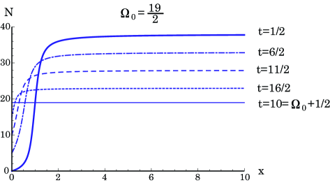
Figure 1: The figure shows $N$ as a function of $x$ with various $t$ for the case $\Omega_{0}=19/2$. The solid, dash-dotted, dashed and dotted curves represent the case $t=1/2$, 3, $11/2$ and 8, respectively. The thin line represents the case $t=\Omega_{0}+1/2\ (=10)$.

In the $B_{ps}$-form framework, the expectation value ${\cal T}_{+}=({\phi}|{\widetilde{\cal T}}_{+}|{\phi})$ is given in the form

$${\cal T}_{+} = \langle{\phi}|{\hat{\cal T}}_{+}|{\phi}\rangle=\langle{\phi}|{\hat{T}}_{+}|{\phi}\rangle$$ (5.76)

$$= z^{*}\cdot\frac{1}{\Gamma}\sum_{n=0}^{2\Omega_{0}-(2t-1)}nx^{n-1}\left(\begin{array}[]{c}2t-1+n\\ n\end{array}\right)$$

$$= z^{*}\cdot\frac{1}{x}\Lambda_{t}(x)\ .$$ (5.77)

It is noted that ${\cal T}_{+}$ is expressed in terms of the product of $z^{*}$ and the function of $x\ (=|z|^{2})$, $\Lambda_{t}(x)/x$. In order to get a transparent understanding for ${\cal T}_{+}$, we introduce a new parameter $(y,y^{*})$:

$$y=z\sqrt{\frac{\Lambda}{x}}=\frac{z}{|z|}\sqrt{\Lambda}\ ,\qquad{\rm i.e.,}\qquad\Lambda=y^{*}y\ .$$ (5.78)

Then, ${\cal T}_{+}$ is expressed as

$${\cal T}_{+}=y^{*}\sqrt{\frac{\Lambda}{x}}\ .$$ (5.79)

After lengthy calculation, we have the relation

$$\frac{\Lambda}{x}=2t+y^{*}y-Y\ ,$$ (5.80)

$$Y=\frac{\displaystyle 2tx^{2\Omega_{0}+1}\left[\left(\frac{1-x}{x}\right)^{2t}\left(\begin{array}[]{c}2\Omega_{0}+1\\ 2t\end{array}\right)-\sum_{n=1}^{2t-1}\left(\frac{1-x}{x}\right)^{n}\left(\begin{array}[]{c}2\Omega_{0}+n\\ n\end{array}\right)\right]}{\displaystyle 1-x^{2\Omega_{0}+1}\sum_{n=1}^{2t-1}\left(\frac{1-x}{x}\right)^{n}\left(\begin{array}[]{c}2\Omega_{0}+n\\ n\end{array}\right)}\ .\qquad$$ (5.87)

Then, ${\cal T}_{\pm}$ can be expressed as

$${\cal T}_{+}=y^{*}\cdot\sqrt{2t+y^{*}y-Y}\ ,\qquad{\cal T}_{-}=\sqrt{2t+y^{*}y-Y}\cdot y\ .$$ (5.88)

The expectation value $N$ is expressed in the form

$$N=(2t-1)+2y^{*}y\ .$$ (5.89)

With the use of the relation (5.39), ${\cal T}_{0}$ is of the form

$${\cal T}_{0}=t+y^{*}y\ .$$ (5.90)

If $Y$ given in the relation (5.87) can be neglected, the set $({\cal T}_{\pm,0})$ reduces to the classical counterpart of the set of the $su(1,1)$-generator ${\hat{T}}_{\pm,0}$, namely, it is the classical counterpart of the Holstein-Primakoff representation. It should be noted that $(y,y^{*})$ is the canonical variable in the boson type. The above feature of the $su(1,1)$-algebra was discussed by the present authors with Kuriyama in detail[5].

6 Approximate expression for the expectation value of the fermion-number operator

In §5, we gave the expectation value of ${\widetilde{N}}$ for $|{\phi})$. The result is too complicated to use it for practical purpose. Then, we must find the approximate expression which is fit for this purpose. As was already mentioned, roughly speaking, in the region where $x$ is sufficiently large, $N$ changes gently, but in the region $x{\stackrel{{\scriptstyle<}}{{\raisebox{-4.30554pt}{$\sim$}}}}2$, especially $x{\stackrel{{\scriptstyle<}}{{\raisebox{-4.30554pt}{$\sim$}}}}1$, it changes steeply. Therefore, it may be impossible to give an approximate expression of $N$ in terms of a well-behaved simple function of $x$ in the whole range $0\leq x<\infty$, but, if the range is limited, it may be possible. Judging from the behavior shown in Fig.1, it may be natural to divide the whole range into two: (1) $0\leq x\leq\gamma_{t}$ and (2) $\gamma_{t}\leq x<\infty$. Here, we conjecture that $\gamma_{t}$ is given in the form

$$\gamma_{t}=\frac{2\Omega_{0}-(2t-1)}{2\Omega_{0}}=1-\frac{2t-1}{2\Omega_{0}}\ (\leq 1)\ .$$ (6.1)

Later, we will give an interpretation of the relation (6.1). We treat the ranges (1) and (2), separately.

First, we introduce the following function for the approximate expression of $\Gamma_{t}(x)$, which is denoted as $\Gamma_{t}^{a}(x)$:

$$\Gamma_{t}(x)=\left\{\begin{array}[]{ll}\displaystyle\left(\frac{1}{1-\alpha x}\right)^{\frac{2t}{\alpha}}\ \left(=\Gamma_{t}^{a_{1}}(x)\right)&{\rm for\ the\ range\ (1)}\\ \displaystyle\left(\begin{array}[]{c}2\Omega_{0}\\ 2t-1\end{array}\right)\left[x^{2\Omega_{0}}\left(\frac{1}{1-\frac{\beta}{x}}\right)^{\frac{1}{2\Omega_{0}\beta}}\right]^{2\Omega_{0}-(2t-1)}\!\!\!\!\!\!\left(=\Gamma_{t}^{a_{2}}(x)\right)&{\rm for\ the\ range\ (2)}\ .\end{array}\right.$$ (6.6)

(6.7)

Here, $\alpha$ and $\beta$ are real parameters which will be determined later. For the form (6.7), we have the following relation:

$$\Gamma_{t}^{a_{1}}(x)=1+2tx+\cdots\ ,\qquad(\alpha x<1)$$ (6.8a)

$$\Gamma_{t}^{a_{2}}(x)=\left(\begin{array}[]{c}2\Omega_{0}\\ 2t-1\end{array}\right)x^{2\Omega_{0}-(2t-1)}\left(1+\frac{2\Omega_{0}-(2t-1)}{2\Omega_{0}}\frac{1}{x}+\cdots\right)\ .\qquad\left(\frac{\beta}{x}<1\right)$$ (6.8d)

(6.8e)

The forms (6.7) are reduced to the forms (5.8) and (5.16), if $x\sim 0$ and $x\rightarrow\infty$, respectively. From the above consideration, it may be understandable that $\Gamma_{t}^{a}(x)$ is a possible approximation of $\Gamma_{t}(x)$. The functions $(1-\alpha x)$ and $(1-\beta/x)$ should not have the points which make $1-\alpha x=0$ and $1-\beta/x=0$ in the ranges $0\leq x\leq\gamma_{t}$ and $\gamma_{t}\leq x<\infty$, respectively. These situations are realized under the condition

$$\alpha<\frac{1}{\gamma_{t}}\ ,\qquad\beta<\gamma_{t}\ .$$ (6.9)

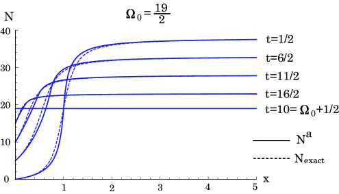
Figure 2: The figure shows $N^{a}$ as a function of $x$ with various $t$ for the case $\Omega_{0}=19/2$. The solid curves represent $N^{a}$ and, for comparison, the exact $N$ are depicted. It is noted that the horizontal scale is different from that of Fig.1.

Through the relation (5.40), we define the approximate form of $\Lambda_{t}(x)$ as follows:

$$\Lambda_{t}^{a}(x)=\frac{x\frac{d\Gamma_{t}^{a}(x)}{dx}}{\Gamma_{t}^{a}(x)}=\left\{\begin{array}[]{ll}\displaystyle\frac{2tx}{1-\alpha x}&{\rm for}\quad 0\leq x\leq\gamma_{t}\ ,\\ \displaystyle(2\Omega_{0}-(2t-1))\left(1-\frac{1}{2\Omega_{0}(x-\beta)}\right)&{\rm for}\quad\gamma_{t}\leq x<\infty\ .\end{array}\right.\ \$$ (6.12)

We require the condition that the functions (6.12) should connect with each other smoothly at $x=\gamma_{t}$:

$$\frac{2t\gamma_{t}}{1-\alpha\gamma_{t}}=(2\Omega_{0}-(2t-1))\left(1-\frac{1}{2\Omega_{0}(\gamma_{t}-\beta)}\right)\ ,$$ (6.13a)

$$\frac{2t}{(1-\alpha\gamma_{t})^{2}}=\frac{2\Omega_{0}-(2t-1)}{2\Omega_{0}(\gamma_{t}-\beta)^{2}}\ .$$ (6.13b)

The condition (6.13) determines $\alpha$ and $\beta$ in the form

$$\alpha=\frac{1}{\gamma_{t}}\left(1-\frac{1}{2\Omega_{0}}\sqrt{\frac{2t}{\gamma_{t}}}-\frac{2t}{2\Omega_{0}}\right)\ (=\alpha_{t})\ ,$$ (6.14a)

$$\beta=\gamma_{t}\left(1-\frac{1}{2\Omega_{0}}\sqrt{\frac{2t}{\gamma_{t}}}-\frac{1}{2\Omega_{0}\gamma_{t}}\right)\ (=\beta_{t})\ .$$ (6.14b)

We can see that $\alpha$ and $\beta$ depend on $t$ and, then, hereafter, we express $\alpha$ and $\beta$ such as $\alpha_{t}$ and $\beta_{t}$. Clearly, they satisfy the condition (6.9). The approximate expression of $N$, $N^{a}$, is given as

$$N^{a}=2t-1+2\Lambda_{t}^{a}(x)\ .$$ (6.15)

Figure 2 shows several concrete cases, together with $N$ shown in the relation (5.39). We can see that the agreement is rather good. Next, we discuss the typical three cases $x=0$, 1 and $x\rightarrow\infty$. The cases $x=0$ and $x\rightarrow\infty$ agree with the exact results shown in the relations (5.73a) and (5.73c), because these two cases are constructed so as to reproduce the exact results. The case $x=1$ is expressed in the form

$$N^{a}=2t-1+2\left(1-\frac{1}{(2t+1)+\left(\sqrt{2t\left(1-\frac{2t-1}{2\Omega_{0}}\right)}-1\right)}\right)(2\Omega_{0}-(2t-1))\ .\quad$$ (6.16)

The exact result (5.73b) can be expressed as

$$N=2t-1+2\left(1-\frac{1}{2t+1}\right)(2\Omega_{0}-(2t-1))\ .$$ (6.17)

The cases $2t=1$ and $2\Omega_{0}$ agree with the exact results, but in the other cases, disagreement with the exact one is not so much as imagined.

Let us discuss the quantity $\gamma_{t}$ which was introduced in the opening paragraph of this section. First, for $t=1/2$, we note the following relation:

$$\Lambda_{1/2}(x)+\Lambda_{1/2}\left(\frac{1}{x}\right)=2\Omega_{0}\ .$$ (6.18)

With the use of the formulae (i)^′ and (ii)^′, we can prove this relation. In (A), also we gave the relation (6.18). This relation tells us that if $\Lambda_{1/2}$ for $0\leq x\leq 1$ is given, we are able to obtain $\Lambda_{1/2}$ for $1\leq x<\infty$ and vice versa. From the above argument, the range $0\leq x<\infty$ is divided by $x=1$; (1) $0\leq x\leq 1$ and (2) $1\leq x<\infty$. In the case $2\Omega_{0}-(2t-1)=0$, i.e., $t=\Omega_{0}+1/2$, $\Lambda_{t=\Omega_{0}+1/2}=0$ and the range $0\leq x<\infty$ is formally divided by $x=0$; (1) $x=0$ and (2) $0\leq x<\infty$. Combining the above two extreme cases with the behavior of $N\ (=2t-1+2\Lambda)$ shown in Fig.1, we conjectured that the range $0\leq x<\infty$ is divided by $x=\gamma_{t}=(2\Omega_{0}-(2t-1))/(2\Omega_{0})$: (1) $0\leq x\leq\gamma_{t}$ and (2) $\gamma_{t}\leq x<\infty$. The parameter $\gamma_{t}$ is the ratio of the number of the single-particle states in ${\overline{P}}$ which can contribute to the fermion-pair formation to the total number of the single-particle states in ${\overline{P}}$. Therefore, if $\gamma_{t}$ is near to 1, the possibility for the fermion-pair formation is large and vice versa. The above is the interpretation of the conjecture for $\gamma_{t}$.

In the framework of our approximation, we generalized the relation (6.18), which can be rewritten as

$$\Lambda_{1/2}(x)=2\Omega_{0}-\Lambda_{1/2}\left(\frac{1}{x}\right)\ .$$ (6.19)

If $1\leq x<\infty$, we have $0\leq 1/x\leq 1$, i.e., $x\cdot(1/x)=1$. We generalize the relation (6.19) to the case of arbitrary value of $t$. If $\gamma_{t}\leq x<\infty$, $\gamma_{t}^{2}/x$ obeys the inequality $0\leq\gamma_{t}^{2}/x\leq\gamma_{t}$, i.e., $x\cdot(\gamma_{t}^{2}/x)=\gamma_{t}^{2}$. Of course, if $t=1/2$, we have $x\cdot(1/x)=1$. Then, the relation (6.12) for $0\leq x\leq\gamma_{t}$ gives

$$\Lambda_{t}^{a_{1}}\left(\frac{\gamma_{t}^{2}}{x}\right)=\frac{2t\cdot\frac{\gamma_{t}^{2}}{x}}{1-\alpha_{t}\cdot\frac{\gamma_{t}^{2}}{x}}\ ,\quad{\rm i.e.,}\quad\frac{\gamma_{t}^{2}}{x}=\frac{\Lambda_{t}^{a_{1}}\left(\frac{\gamma_{t}^{2}}{x}\right)}{\alpha_{t}\Lambda_{t}^{a_{1}}\left(\frac{\gamma_{t}^{2}}{x}\right)+2t}\ .$$ (6.20)

The relation (6.20) leads to

$$x=\gamma_{t}^{2}\left(\alpha_{t}+\frac{2t}{\Lambda_{t}^{a_{1}}\left(\frac{\gamma_{t}^{2}}{x}\right)}\right)\ .\qquad(\gamma_{t}\leq x<\infty)$$ (6.21)

Therefore, the relation (6.12) for $\gamma_{t}\leq x<\infty$ can be rewritten as

$$\Lambda_{t}^{a_{2}}(x) = 2\Omega_{0}\gamma_{t}\left(1-\frac{1}{2\Omega_{0}(x-\beta_{t})}\right)$$ (6.22)

$$= 2\Omega_{0}\gamma_{t}\Biggl{(}1-\frac{1}{2\Omega_{0}\Bigl{[}\gamma_{t}^{2}\Bigl{(}\alpha_{t}+\frac{2t}{\Lambda_{t}^{a_{1}}\left(\frac{\gamma_{t}^{2}}{x}\right)}\Bigl{)}-\beta_{t}\Bigl{]}}\Biggl{)}\ .$$

With the use of the explicit expressions of $\alpha_{t}$ and $\beta_{t}$ given in the relation (6.14), we have the following:

$$\Lambda_{t}^{a_{2}}(x)=2\Omega_{0}\gamma_{t}\left(1-\frac{\Lambda_{t}^{a_{1}}\left(\frac{\gamma_{t}^{2}}{x}\right)}{(1-2t\gamma_{t})\Lambda_{t}^{a_{1}}\left(\frac{\gamma_{t}^{2}}{x}\right)+2t\cdot 2\Omega_{0}}\right)\ .$$ (6.23)

If $\Lambda_{t}^{a_{1}}$ is given, $\Lambda_{t}^{a_{2}}$ is obtained by the relation (6.23). In the case $t=1/2$, $\Lambda_{1/2}^{a_{2}}(x)$ is expressed as

$$\Lambda_{1/2}^{a_{2}}(x)=2\Omega_{0}-\Lambda_{1/2}^{a_{1}}\left(\frac{1}{x}\right)\ .$$ (6.24)

Also, in the case $t=\Omega_{0}+1/2$, i.e., $2\Omega_{0}-(2t-1)=0$, we have

$$\Lambda_{t=\Omega_{0}+1/2}^{a_{2}}(x)=0\ .$$ (6.25)

In the exact case for $t>1/2$, numerically, the relation corresponding to the relation (6.23) may be presented, but, in analytical form, it may be impossible.

Finally, we will investigate the parameters $\alpha_{t}$ and $\beta_{t}$ given in the relations (6.14a) and (6.14b), respectively. Both relations are rewritten as

$$\alpha_{t}=1-\frac{1}{2\Omega_{0}-(2t-1)}\left(\sqrt{\frac{2\Omega_{0}\cdot 2t}{2\Omega_{0}-(2t-1)}}+1\right)\ ,$$ (6.26a)

$$\beta_{t}=1-\frac{1}{2\Omega_{0}}\left(2t+\sqrt{\frac{2t}{2\Omega_{0}}(2\Omega_{0}-(2t-1))}\right)\ .$$ (6.26b)

The above expressions tell us

$$\alpha_{t}<1\ ,\qquad\beta_{t}<1\ .$$ (6.27)

In the $su(1,1)$-algebraic model, we have $\alpha_{t}=1$, which is realized in the case with $\Omega_{0}\rightarrow\infty$ and finite value of $t$. However, in our present model, $\Omega_{0}$ and $t$ are finite and $\alpha_{t}$ should obey the condition (6.27). We do not know any model related to $\beta_{t}$ and, then, any comparison is impossible. Since $\alpha_{t}$ is decreasing for $2t$, the maximum value of $\alpha_{t}$ is given as

$$\alpha_{1/2}=1-\frac{1}{\Omega_{0}}\ ,\qquad\gamma_{1/2}=1\ .$$ (6.28)

At the point $2t=2t^{0}$, which will be later discussed, $\alpha_{t}$ vanishes $(\alpha_{t^{0}}=0$). After $\alpha_{t^{0}}=0$, $\alpha_{t}$ can change to $-\infty$:

$$\alpha_{\Omega_{0}}=-2\Omega_{0}\quad(\gamma_{\Omega_{0}}=\frac{1}{2\Omega_{0}})\ ,\qquad\alpha_{\Omega_{0}+1/2}\rightarrow-\infty\quad(\gamma_{\Omega_{0}+1/2}=0)\ .$$ (6.29)

The quantity $\Lambda_{t}^{a_{1}}(x)$ in the range $\alpha_{1/2}>\alpha_{t}>0$ is of the type similar to that of the $su(1,1)$-algebraic model: $\Lambda_{t}^{a_{1}}(x)=2tx/(1-|\alpha_{t}|x)$. At $\alpha_{t^{0}}=0$, $\Lambda_{t}^{a_{1}}(x)=2t^{0}x$ and in the range $0>\alpha_{t}>-\infty$, $\Lambda_{t}^{a_{1}}(x)=2tx/(1+|\alpha_{t}|x)$. If $2\Omega_{0}$ and $2t$ can change continuously, $\alpha_{t}=0$ itself has own meaning. But, they are integers and we treat $\alpha_{t}=0$ as an auxiliary condition. It leads us to a certain cubic equation for $2t$ with one real solution and it is given as

$$2t^{0}=2\Omega_{0}+\frac{1}{3}-(2\Omega_{0})^{\frac{2}{3}}\left[\sqrt[3]{\frac{1}{2}(A+B)}-\sqrt[3]{\frac{1}{2}(A-B)}\right]\ ,$$

$$A=\sqrt{\left(1-\frac{5}{54\Omega_{0}}\right)\left(1+\frac{1}{2\Omega_{0}}\right)}\ ,\qquad B=1+\frac{1}{6\Omega_{0}}-\frac{1}{54\Omega_{0}^{2}}\ .$$ (6.30a)

The expression (6.30) is approximated in the form

$$2t^{0}=2\Omega_{0}-(2\Omega_{0})^{\frac{2}{3}}+\frac{1}{3}(2\Omega_{0})^{\frac{1}{3}}+\frac{1}{3}-\frac{10}{81}(2\Omega_{0})^{-\frac{1}{3}}\ .$$ (6.30b)

As is conjectured in the relation (6.30), $2t^{0}$ cannot be expected to be integer. Therefore, two integers $2t^{+}$ and $2t^{-}$ ($t^{+}<t^{-}$) which are the nearest to $2t^{0}$ must be searched: $\alpha_{t}>0$ for $1\leq 2t\leq 2t^{+}$ and $\alpha_{t}<0$ for $2t^{-}\leq 2t\leq 2\Omega_{0}+1$. For this searching, the relation (6.30) is useful. For example, in the case $2\Omega_{0}=19$, the relations (6.30) and (6.30b) give us $2t^{0}\sim 13.0235$ and 13.0562, respectively and, therefore, $2t^{+}=13$ and $2t^{-}=14$. For them, we have $\alpha_{t^{+}}=8.5460\times 10^{-3}\ (>0)$ and $\alpha_{t^{-}}=-0.2764\ (<0)$. The treatment of $\beta_{t}$ is rather simple. As is clear from the relation (6.26b), the maximum value of $\beta_{t}$ is also given in the case $t=1/2$:

$$\beta_{1/2}=1-\frac{1}{\Omega_{0}}\ .$$ (6.31)

Then, gradually decreases, at the point $2t=2\Omega_{0}-2$, $\beta_{\Omega_{0}-1}$ is given as

$$\beta_{\Omega_{0}-1}=\frac{1}{\Omega_{0}}\left(1-\frac{1}{2}\sqrt{3\left(1-\frac{1}{2\Omega_{0}}\right)}\right)\ (>0)\ .$$ (6.32)

At the point $2t=2\Omega_{0}-1$, $\beta_{\Omega_{0}-1/2}$ is given as

$$\beta_{\Omega_{0}-1/2}=-\frac{1}{2\Omega_{0}}\left(\sqrt{2-\frac{1}{\Omega_{0}}}-1\right)\ (<0)\ .$$ (6.33)

At the terminal points $2t=2\Omega_{0}$ and $2\Omega_{0}+1$, we have

$$\beta_{\Omega_{0}}=\beta_{\Omega_{0}+1/2}=-\frac{1}{2\Omega_{0}}\ .$$ (6.34)

We can see that the sign of $\beta_{t}$ changes between $2t=2\Omega_{0}-2$ and $2\Omega_{0}-1$. The point which satisfies $\beta_{t}=0$ is given at $2t=2t^{0}{}^{\prime}$ shown as

$$2t^{0}{}^{\prime}=2\Omega_{0}-\frac{2\Omega_{0}-1+2\Omega_{0}\sqrt{5+\frac{1}{\Omega_{0}}+\frac{1}{4\Omega_{0}^{2}}}}{2(2\Omega_{0}+1)}\ .$$ (6.35)

7 A simple example of many-fermion model obeying the pseudo $su(1,1)$-algebra

In next three sections, we intend to discuss an example of the application of the idea developed until the present. This section will be devoted to presenting a simple many-fermion model aimed at the application. As an illustrative example of our idea, first, we give a short summary of the “damped and amplified oscillator.” The starting Hamiltonian is the simplest, i.e., the harmonic oscillator:

$${\hat{H}}_{b}=\omega{\hat{b}}^{*}{\hat{b}}\ .\qquad(\omega\ ;\ {\rm frequency})$$ (7.1)

Here, $({\hat{b}},{\hat{b}}^{*})$ denotes boson operator. As an auxiliary degree of freedom for the “damping and amplifying,” new boson $({\hat{a}},{\hat{a}}^{*})$ is introduced. The Hamiltonian for $({\hat{a}},{\hat{a}}^{*})$ is also the harmonic oscillator type:

$${\hat{H}}_{a}=\omega{\hat{a}}^{*}{\hat{a}}\ .$$ (7.2)

Further, as for the interaction between both degrees of freedom, the following form is adopted:

$${\hat{V}}_{ab}=-i\gamma({\hat{a}}^{*}{\hat{b}}^{*}-{\hat{b}}{\hat{a}})\ .\qquad(\gamma\ ;\ {\rm constant})$$ (7.3)

The idea presented in Ref.6 is to adopt the Hamiltonian

$${\hat{H}}={\hat{H}}_{b}-{\hat{H}}_{a}+{\hat{V}}_{ba}\ .$$ (7.4)

By treating ${\hat{H}}$ appropriately, we can describe the “damped and amplified oscillation” in the conservative form. It should be noted that, for the Hamiltonian (7.4), the form $({\hat{H}}_{b}+{\hat{H}}_{a}+{\hat{V}}_{ba})$ is not adopted. It shows that the Hamiltonian (7.4) is not the energy of the entire system, but the generator for time-evolution. This is a significant feature of this approach. With the use of ${\hat{T}}_{\pm}$ defined in the relation (2.10), ${\hat{H}}$ can be expressed as

$${\hat{H}}=2\omega\left({\hat{T}}-\frac{1}{2}\right)-i\gamma\left({\hat{T}}_{+}-{\hat{T}}_{-}\right)\ .$$ (7.5)

Here, ${\hat{T}}$ is defined as

$${\hat{T}}=-\frac{1}{2}({\hat{a}}^{*}{\hat{a}}-{\hat{b}}^{*}{\hat{b}})+\frac{1}{2}\ ,$$ (7.6a)

$${\hat{\mib T}}^{2}={\hat{T}}\left({\hat{T}}-1\right)\ ,\qquad[\ {\hat{T}}_{\pm,0}\ ,\ {\hat{T}}\ ]=0\ .$$ (7.6b)

By using the mixed-mode coherent states for the $su(1,1)$-algebra, the present authors, with Kuriyama, have investigated extensively the Hamiltonian (7.5) and its variations [5].

The above illustrative example teaches us the following: In order to treat the system such as the “damped and amplified oscillator” in an isolated system, so-called phase space doubling is required. The idea of the phase space doubling occupies main part of the thermo-field dynamics formalism [8]. Then, the original intrinsic oscillator expressed in terms of the boson $({\hat{b}},{\hat{b}}^{*})$ and the “external environment” expressed in terms of the boson $({\hat{a}},{\hat{a}}^{*})$ appear. The interaction between both systems is introduced. We will apply the above consideration to a simple many-fermion system.

We make the following translation into the fermion system:

$$({\hat{b}},{\hat{b}}^{*})\rightarrow({\tilde{c}}_{\bar{\alpha}},{\tilde{c}}_{\bar{\alpha}}^{*})\ ,\qquad({\hat{a}},{\hat{a}}^{*})\rightarrow({\tilde{c}}_{\alpha},{\tilde{c}}_{\alpha}^{*})\ ,$$ (7.7)

$${\hat{T}}-\frac{1}{2}\rightarrow{\widetilde{\cal T}}=-\frac{1}{2}\sum_{\alpha}({\tilde{c}}_{\alpha}^{*}{\tilde{c}}_{\alpha}-{\tilde{c}}_{\bar{\alpha}}^{*}{\tilde{c}}_{\bar{\alpha}})\ (=-{\widetilde{R}}_{0})\ ,\qquad{\hat{T}}_{\pm}\rightarrow{\widetilde{\cal T}}_{\pm}\ ,$$ (7.8)

$$\omega\ ({\rm frequency})\rightarrow\varepsilon\ (\textrm{single-particle energy})\ .$$ (7.9)

Here, ${\widetilde{\cal T}}$ is introduced in the relation (4.10) and the relation (4.11) suggests us the relation $[\ {\widetilde{\cal T}}\ ,\ {\widetilde{\cal T}}_{\pm}\ ]=0$. Under the above translation, our Hamiltonian is expressed in the form

$${\widetilde{H}}=2\varepsilon{\widetilde{\cal T}}-i\gamma\left({\widetilde{\cal T}}_{+}-{\widetilde{\cal T}}_{-}\right)\ .$$ (7.10)

It may be clear that we have the translation

$${\hat{H}}_{b}\rightarrow{\widetilde{H}}_{\overline{P}}=\varepsilon{\widetilde{N}}_{\overline{P}}\ ,\quad{\widetilde{N}}_{\overline{P}}=\sum_{\alpha}{\tilde{c}}_{\bar{\alpha}}^{*}{\tilde{c}}_{\bar{\alpha}}\ ,\qquad{\hat{H}}_{a}\rightarrow{\widetilde{H}}_{P}=\varepsilon{\widetilde{N}}_{P}\ ,\quad{\widetilde{N}}_{P}=\sum_{\alpha}{\tilde{c}}_{\alpha}^{*}{\tilde{c}}_{\alpha}\ .$$ (7.11)

The original intrinsic Hamiltonian ${\widetilde{H}}_{\overline{P}}$ may be the simplest in many-fermion systems and our aim is to describe this system in the “external environment.” The Hamiltonian (7.10) was set up under an idea analogous to that in the case (7.5). However, it may be permitted to regard the Hamiltonian (7.10) as the energy of the entire system. Concerning this point, we will discuss the possibility in §11. It may be important to see that the conventional pairing Hamiltonian and the present one are expressed in terms of the $su(2)$-generators, ${\widetilde{S}}_{\pm,0}$, but differently from the former, the latter does not commute with the total fermion-number operator. In this sense, the use of the state (1.1) for the variational treatment in the pairing Hamiltonian is justified by the symmetry breaking. On the other hand, the use of the state (5.1) (or (5.2)) may be natural as a possible trial state for the variation without any comment such as the symmetry breaking.

Our basic idea is to describe the Hamiltonian (7.10) in the framework of the time-dependent variational method:

$$\delta\int({\phi}|i\partial_{\tau}-{\widetilde{H}}|{\phi})d\tau=0\ .$$ (7.12)

Here, the state $|{\phi})$ is used for the trial state of the variation. In order to avoid the confusion between the time variable and the quantum number $t$, we will use $\tau$ for the time variable. For the relation (7.12), the following are useful:

$$\delta\int({\phi}|i\partial_{\tau}|{\phi})d\tau=\frac{i}{2}\int\left(\delta z^{*}\cdot{\dot{z}}-\delta z\cdot{\dot{z}}^{*}\right)\left(\frac{\partial{\cal T}_{+}}{\partial z^{*}}+\frac{\partial{\cal T}_{-}}{\partial z}\right)d\tau\ ,$$ (7.13)

$$\delta\int({\phi}|{\widetilde{H}}|{\phi})d\tau=\int\left(\delta z^{*}\frac{\partial{\cal H}}{\partial z^{*}}+\delta z\frac{\partial{\cal H}}{\partial z}\right)d\tau\ .$$ (7.14)

Here, ${\cal T}_{\pm}$ is given in the relation (5.76) and ${\cal H}$ is defined as

$${\cal H}={\cal H}(z^{*},z)=({\phi}|{\widetilde{H}}{|{\phi})}\ .$$ (7.15)

Then, the relations (7.12)-(7.14) give us

$$i{\dot{z}}\frac{1}{2}\left(\frac{\partial{\cal T}_{+}}{\partial z^{*}}+\frac{\partial{\cal T}_{-}}{\partial z}\right)=\frac{\partial{\cal H}}{\partial z^{*}}\ ,\qquad-i{\dot{z}}^{*}\frac{1}{2}\left(\frac{\partial{\cal T}_{+}}{\partial z^{*}}+\frac{\partial{\cal T}_{-}}{\partial z}\right)=\frac{\partial{\cal H}}{\partial z}\ .$$ (7.16)

For the relation (7.16), ${\cal H}$ is adopted in the following form:

$${\cal H}=\varepsilon(2t-1)-i\gamma\left({\cal T}_{+}-{\cal T}_{-}\right)=\varepsilon(2t-1)-\gamma\cdot i(z^{*}-z)\frac{\Lambda_{t}(x)}{x}\ .$$ (7.17)

Under the Hamiltonian (7.17), the relation (7.16) is reduced to the differential equation

$${\dot{z}}=-\gamma\left[1-\frac{z^{2}}{x}\left(1-\frac{\Lambda_{t}(x)}{x\Lambda^{\prime}_{t}(x)}\right)\right]\ ,\qquad{\dot{z}}^{*}=-\gamma\left[1-\frac{z^{*2}}{x}\left(1-\frac{\Lambda_{t}(x)}{x\Lambda^{\prime}_{t}(x)}\right)\right]\ .\qquad$$ (7.18)

Here, $\Lambda_{t}^{\prime}(x)$ denotes the derivative of $\Lambda_{t}(x)$ for $x$.

The relation (7.18) forms our basic framework for describing the time-evolution. In order to give the physical interpretation of the relation (7.18), we examine the case $\Lambda_{t}^{a_{1}}(x)$. In this case, the relation (7.18) becomes

$${\dot{z}}=-\gamma(1-\alpha_{t}z^{2})\ ,\qquad{\dot{z}}^{*}=-\gamma(1-\alpha_{t}z^{*}{}^{2})\ .$$ (7.19)

If $z$ is expressed as $z=u+iv$ ($u$, $v$: real), we have

$${\dot{u}}=-\gamma(1-\alpha_{t}u^{2}+\alpha_{t}v^{2})\ ,\qquad{\dot{v}}=2\gamma\alpha_{t}uv\ .$$ (7.20)

If we eliminate $v$ from the relation (7.20), the following equation is derived:

$${\ddot{u}}=4\gamma^{2}\alpha_{t}^{2}u\left(\frac{1}{\alpha_{t}}-u^{2}\right)+6\alpha_{t}u{\dot{u}}\ .$$ (7.21)

If the relation (7.21) is interpreted in Newton mechanics, a mass point with mass$=1$ moves in the one-dimensional space under the external force $4\gamma^{2}\alpha_{t}^{2}u(1/\alpha_{t}-u^{2})$ and the velocity-dependent force $6\alpha_{t}u{\dot{u}}$. The force $4\gamma^{2}\alpha_{t}^{2}u(1/\alpha_{t}-u^{2})$ is expressed in terms of the potential energy $V(u)$:

$$4\gamma^{2}\alpha_{t}^{2}u\left(\frac{1}{\alpha_{t}}-u^{2}\right)=-\frac{dV(u)}{du}\ ,\qquad V(u)=-4\gamma^{2}\left(\frac{1}{2}\alpha_{t}u^{2}-\frac{1}{4}\alpha_{t}^{2}u^{4}\right)\ .$$ (7.22)

The cases $\alpha_{t}>0$ and $\alpha_{t}<0$ correspond to double well-like and single well-like potentials, respectively and the case $\alpha_{t}=0$ to no external force. Existence of the velocity-dependent force suggests that our model enable us to describe the dissipation phenomena in many-fermion system. If we can solve the equation of motion (7.21), $u$ can be determined as a function of $\tau$ and the second of the relation (7.20) gives us the following form:

$$v(\tau)=e^{2\gamma\alpha_{t}\int^{\tau}u(\tau^{\prime})d\tau^{\prime}}\ .$$ (7.23)

Here, we omitted the initial condition for $u$ and $v$. Thus, we are able to obtain $u(\tau)$ and $v(\tau)$ and, then, $x$ is determined as a function of $\tau$:

$$x(\tau)=u(\tau)^{2}+v(\tau)^{2}\ .$$ (7.24)

The case $\Lambda_{t}^{a_{2}}(x)$ is not so simple as the case $\Lambda_{t}^{a_{1}}(x)$, because, in classical mechanics, we cannot find any simple example analogous to this case. The above is an outline of our model discussed in next sections.

Finally, we give the expectation values of ${\widetilde{N}}_{\overline{P}}$ and ${\widetilde{N}}_{P}$ for $|{\phi})$, $N_{\overline{P}}$ and $N_{P}$:

$$N_{\overline{P}}=2t-1+\Lambda_{t}(x)\ ,$$ (7.25a)

$$N_{P}=\Lambda_{t}(x)\ .$$ (7.25b)

The expectation value of ${\widetilde{N}}(={\widetilde{N}}_{\overline{P}}+{\widetilde{N}}_{P})$ is given as $N=(2t-1+\Lambda_{t}(x))+\Lambda_{t}(x)$ and it is nothing but the result (5.39).

8 Various properties of $\Lambda_{t}^{a_{1}}(x)$ for describing its time-dependence

Let us investigate various properties of $\Lambda_{t}^{a_{1}}(x)$. First, we notice that the present system is of two-dimension and, then, there exist two constants of motion. One is the quantum number $t$ and the second, which will be denoted as $\kappa$, is given through the relation

$$i(z^{*}-z)\frac{\Lambda_{t}(x)}{x}=2\kappa\ .$$ (8.1)

It may be self-evident, because ${\cal H}$ itself shown in the relation (7.17) is a constant of motion. If $z$ is expressed in the form $z=u+iv$, we have

$$i(z^{*}-z)=2v\ .$$ (8.2)

The relation (8.1) leads to

$$v=\frac{\kappa}{y}\ ,\qquad y=\frac{\Lambda_{t}(x)}{x}\ .\qquad(x=|z|^{2}=u^{2}+v^{2}\ ,\quad y\geq 0)$$ (8.3)

Inversely, $x$ can be expressed as a function of $y$:

$$x=f_{t}(y)\ .$$ (8.4)

Then, $u$ can be given in the form

$$u=\pm\sqrt{x-v^{2}}=\pm\frac{1}{y}\sqrt{y^{2}f_{t}(y)-\kappa^{2}}\ .$$ (8.5)

The sign $+$ or $-$ may be appropriately chosen. Later, we will discuss this problem. As is clear in the above argument, $(u,v)$ and also $x$ are functions of $y$. Since $u^{2}\geq 0$, the relation (8.5) gives us the inequality

$$y^{2}f_{t}(y)\geq\kappa^{2}\ .$$ (8.6)

The inequality (8.6) suggests us that the value of $y$ cannot vary freely. We will apply the above scheme to the cases $\Lambda_{t}^{a_{1}}(x)$.

For the case $\Lambda_{t}(x)/x=\Lambda_{t}^{a_{1}}(x)/x=2t/(1-\alpha_{t}x)$, we have

$$x=f_{t}(y)=\frac{1}{\alpha_{t}}\left(1-\frac{2t}{y}\right)\ ,\quad{\rm i.e.,}\quad\Lambda_{t}^{a_{1}}(x)=\frac{1}{\alpha_{t}}(y-2t)\ .$$ (8.7)

The relation (8.7) is applicable in the range $0\leq x\leq\gamma_{t}$. In §10, this point will be discussed. Then, the inequality (8.6) is reduced to

$$\frac{1}{\alpha_{t}}\cdot y(y-2t)\geq\kappa^{2}\ ,\qquad\qquad\qquad\qquad\qquad\qquad$$ (8.8)

i.e.,

$$w=\left\{\begin{array}[]{ll}+y(y-2t)\geq\rho^{2}\ ,&\qquad(\alpha_{t}>0)\\ -y(y-2t)\geq\rho^{2}\ ,&\qquad(\alpha_{t}<0)\end{array}\right.$$ (8.11)

$$\rho=\sqrt{|\alpha_{t}|}\kappa\ .$$ (8.12)

The behavior of the relation (8.11) is depicted in Fig. 3.

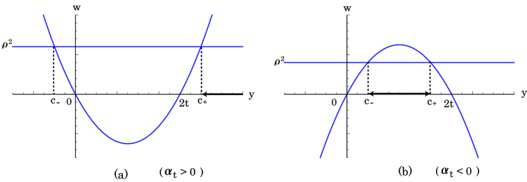
Figure 3: The figures shows the inequality in (8.11) schematically with $\Omega_{0}=19/2$: (a) $t=5/2$, then $\alpha_{t}\approx 0.766\ (>0)$ (b) $t=15/2$, then $\alpha_{t}\approx-0.710\ (<0)$.

In Fig.3, we can find out the following restriction to $y$:

$$y\geq c_{+}\ ,\quad{\rm i.e.}\quad y\geq\frac{1}{2}(c_{+}+c_{-})+\frac{1}{2}(c_{+}-c_{-})\ ,\quad(\alpha_{t}>0)$$ (8.13a)

$$c_{-}\leq y\leq c_{+}\ ,\quad{\rm i.e.,}\quad\frac{1}{2}(c_{+}+c_{-})-\frac{1}{2}(c_{+}-c_{-})\leq y\leq\frac{1}{2}(c_{+}+c_{-})+\frac{1}{2}(c_{+}-c_{-})\ .$$

$$\qquad\qquad\qquad\qquad\qquad\qquad\qquad\qquad\qquad\qquad\qquad\qquad\qquad\qquad(\alpha_{t}<0)$$ (8.13b)

Here, $c_{\pm}$ denote solutions of quadratic equation

$$y^{2}-2ty-\rho^{2}=0\ ,\qquad\ (\alpha_{t}>0)$$ (8.14a)

$$-y^{2}+2ty-\rho^{2}=0\ .\qquad(\alpha_{t}<0)$$ (8.14b)

The above equation is obtained by equating both sides of the inequality (8.11). Therefore, with the use of new variable $\chi$, $y$ can be parametrized in the form

$$y=\frac{1}{2}(c_{+}+c_{-})+\frac{1}{2}(c_{+}-c_{-})\cosh\chi\ ,\qquad(\alpha_{t}>0)$$ (8.15a)

$$y=\frac{1}{2}(c_{+}+c_{-})+\frac{1}{2}(c_{+}-c_{-})\cos\chi\ .\qquad\ \ (\alpha_{t}<0)$$ (8.15b)

In §10, we will discriminate between the former (8.15a) and the later (8.15b) in terms of the notations $y_{+}$ and $y_{-}$. With the use of Eq.(8.15), $u$ and $v$ can be expressed as follows:

$$u=\left\{\begin{array}[]{l}\pm\frac{1}{\sqrt{|\alpha_{t}|}}\cdot\frac{1}{y}\sqrt{(y-c_{+})(y-c_{-})}=\pm\frac{1}{\sqrt{|\alpha_{t}|}}\cdot\frac{1}{y}\cdot\frac{1}{2}(c_{+}-c_{-})|\sinh\chi|\ ,\ (\alpha_{t}>0)\\ \pm\frac{1}{\sqrt{|\alpha_{t}|}}\cdot\frac{1}{y}\sqrt{(c_{+}-y)(y-c_{-})}=\pm\frac{1}{\sqrt{|\alpha_{t}|}}\cdot\frac{1}{y}\cdot\frac{1}{2}(c_{+}-c_{-})|\sin\chi|\ ,\ \ (\alpha_{t}<0)\end{array}\right.\qquad$$ (8.18)

$$v=\frac{1}{\sqrt{|\alpha_{t}|}}\cdot\frac{\rho}{y}\ .\qquad(\alpha_{t}\neq 0)$$ (8.19)

By substituting Eq.(8.15) into the relation (8.7), $x$ can be expressed in terms of $\cosh\chi$ and $\cos\chi$. Then, we can express $\Lambda_{t}^{a_{1}}(x)=2tx/(1-\alpha_{t}x)$ as a function of $\cosh\chi$ and $\cos\chi$.

Since Eq.(8.14) gives us the solutions $c_{\pm}=t\pm\sqrt{t^{2}+\rho^{2}}$ for $\alpha_{t}>0$ and $c_{\pm}=t\pm\sqrt{t^{2}-\rho^{2}}$ for $\alpha_{t}<0$, the relation (8.15) can be expressed as

$$y=\left\{\begin{array}[]{ll}t+\sqrt{t^{2}+\rho^{2}}\cosh\chi\ ,&\quad(\alpha_{t}>0)\\ t+\sqrt{t^{2}-\rho^{2}}\cos\chi\ ,&\quad(\alpha_{t}<0)\end{array}\right.$$ (8.22)

Then, $u$ and $v$ are obtained in the form

$$u=\left\{\!\!\begin{array}[]{l}\displaystyle\pm\frac{1}{\sqrt{|\alpha_{t}|}}\cdot\frac{\sqrt{t^{2}+\rho^{2}}|\sinh\chi|}{t+\sqrt{t^{2}+\rho^{2}}\cosh\chi}\\ \displaystyle\pm\frac{1}{\sqrt{|\alpha_{t}|}}\cdot\frac{\sqrt{t^{2}-\rho^{2}}|\sin\chi|}{t+\sqrt{t^{2}-\rho^{2}}\cos\chi}\end{array}\right.\!\!,\ \ v=\left\{\!\!\begin{array}[]{ll}\displaystyle\frac{1}{\sqrt{|\alpha_{t}|}}\cdot\frac{\rho}{t+\sqrt{t^{2}+\rho^{2}}\cosh\chi}\ ,&(\alpha_{t}>0)\\ \displaystyle\frac{1}{\sqrt{|\alpha_{t}|}}\cdot\frac{\rho}{t+\sqrt{t^{2}-\rho^{2}}\cos\chi}\ .&(\alpha_{t}<0)\end{array}\right.$$ (8.27)

We can express $z$ as the function of $\rho$ and $\chi$. The quantity $x$ is obtained in the form

$$x=\frac{1}{\alpha_{t}}\cdot\frac{\sqrt{t^{2}+\rho^{2}}\cosh\chi-t}{\sqrt{t^{2}+\rho^{2}}\cosh\chi+t}\ ,\qquad(\alpha_{t}>0)$$ (8.29a)

$$x=\frac{1}{\alpha_{t}}\cdot\frac{\sqrt{t^{2}-\rho^{2}}\cos\chi-t}{\sqrt{t^{2}-\rho^{2}}\cos\chi+t}\ .\ \ \qquad(\alpha_{t}<0)$$ (8.29b)

Thus, we have the following form for $\Lambda_{t}^{a_{1}}(x)$:

$$\Lambda_{t}^{a_{1}}(x)=\frac{1}{\alpha_{t}}(\sqrt{t^{2}+\rho^{2}}\cosh\chi-t)\ ,\qquad(\alpha_{t}>0)$$ (8.30a)

$$\Lambda_{t}^{a_{1}}(x)=\frac{1}{\alpha_{t}}(\sqrt{t^{2}-\rho^{2}}\cos\chi-t)\ ,\ \qquad(\alpha_{t}<0)$$ (8.30b)

It may be necessary for determining the time-dependence of $\Lambda_{t}^{a_{1}}(x)$ to investigate the behavior of $\chi$ for the time.

The starting variables for describing the present model are $u$ and $v$. As is shown in the relations (8.18) and (8.19), the new variables are $\rho$ and $\chi$. Depending on $\alpha_{t}>0$ and $\alpha_{t}<0$, the connection to $(u,v)$ is different from each other. However, $\rho$ is a constant of motion and ${\cal H}$ can be expressed as

$${\cal H}=\varepsilon(2t-1)-\frac{2\gamma}{\sqrt{|\alpha_{t}|}}\cdot\rho\ ,\qquad{\dot{\rho}}=0\ .$$ (8.31)

Therefore, the time-dependence of $(u,v)$ is given through $y$ which is a function of $\chi$. First, we notice the relation

$${\dot{x}}={\dot{z}}^{*}z+z^{*}{\dot{z}}=-2\gamma(1-\alpha_{t}x)\cdot u\ .$$ (8.32)

Here, we used relation (7.19). With the use of the relation (8.32), we have ${\dot{y}}$ in the following form:

$${\dot{y}}=\frac{d}{dx}\left(\frac{\Lambda_{t}^{a_{1}}(x)}{x}\right)\cdot{\dot{x}}=-2\gamma\alpha_{t}y\cdot u\ ,$$ (8.33)

i.e.,

$${\dot{y}}=\left\{\begin{array}[]{ll}\mp 2\gamma\sqrt{|\alpha_{t}|}\cdot\frac{1}{2}(c_{+}-c_{-})|\sinh\chi|\ ,&\quad(\alpha_{t}>0)\\ \mp 2\gamma\sqrt{|\alpha_{t}|}\cdot\frac{1}{2}(c_{+}-c_{-})|\sin\chi|\ .&\quad(\alpha_{t}<0)\end{array}\right.$$ (8.36)

On the other hand, the relation (8.15) gives us ${\dot{y}}$ in the form

$${\dot{y}}=\left\{\begin{array}[]{ll}+\frac{1}{2}(c_{+}-c_{-})\sinh\chi\cdot{\dot{\chi}}\ ,&\quad(\alpha_{t}>0)\\ -\frac{1}{2}(c_{+}-c_{-})\sin\chi\cdot{\dot{\chi}}\ .&\quad(\alpha_{t}<0)\end{array}\right.$$ (8.39)

Combining the relations (8.36) and (8.39), ${\dot{\chi}}$ is obtained:

$${\dot{\chi}}=\mp 2\gamma\sqrt{|\alpha_{t}|}\cdot\frac{|\sinh\chi|}{\sinh\chi}=\left\{\begin{array}[]{ll}\mp 2\gamma\sqrt{|\alpha_{t}|}&\quad{\rm for}\ \ \chi>0\ ,\\ \pm 2\gamma\sqrt{|\alpha_{t}|}&\quad{\rm for}\ \ \chi<0\ ,\end{array}\right.\quad(\alpha_{t}>0)$$ (8.40c)

$${\dot{\chi}}=\pm 2\gamma\sqrt{|\alpha_{t}|}\cdot\frac{|\sin\chi|}{\sin\chi}=\left\{\begin{array}[]{ll}\pm 2\gamma\sqrt{|\alpha_{t}|}&\quad{\rm for}\ \ \chi>0\ ,\\ \mp 2\gamma\sqrt{|\alpha_{t}|}&\quad{\rm for}\ \ \chi<0\ ,\end{array}\right.\quad(\alpha_{t}<0)$$ (8.40f)

Our final aim is to present the time-dependence of $\Lambda_{t}^{a_{1}}(x)$, which is also a function of $y$. The quantity $y$ contains $\cosh\chi$ or $\cos\chi$. As can be seen in the relation (8.40), $\chi$ is given in the following two cases:

$${\rm(i)}\quad\chi=\chi_{+}=+2\gamma\sqrt{|\alpha_{t}|}\cdot\tau+\chi_{+}^{0}\ ,$$ (8.41a)

$${\rm(ii)}\quad\chi=\chi_{-}=-2\gamma\sqrt{|\alpha_{t}|}\cdot\tau-\chi_{-}^{0}\ .$$ (8.41b)

Here, $\pm\chi_{\pm}^{0}$ denote the initial values of $\chi_{\pm}$ ($\tau=0$). Then, we have

$$\cosh\chi_{+}=\cosh(2\gamma\sqrt{|\alpha_{t}|}\cdot\tau+\chi_{+}^{0})\ ,\qquad\cosh\chi_{-}=\cosh(2\gamma\sqrt{|\alpha_{t}|}\cdot\tau+\chi_{-}^{0})\ .$$ (8.42)

If $\chi_{+}^{0}=\chi_{-}^{0}$, the case (ii) is nothing but the case (i). The case $\cos\chi$ is also in the same situation as the above. The above argument suggests us that it may be enough to adopt the case (i):

$${\dot{\chi}}=+2\gamma\sqrt{|\alpha_{t}|}\ ,\quad{\rm i.e.,}\quad\chi=2\gamma\sqrt{|\alpha_{t}|}\cdot\tau+\chi^{0}\ .\quad(\chi^{0}\ :\ {\rm constant})$$ (8.43)

The above argument gives us the time-dependence of $\Lambda_{t}^{a_{1}}(x)$. Further, this procedure suggests the following form for $u$:

$$u=\frac{1}{\sqrt{|\alpha_{t}|}}\cdot\frac{\sqrt{t^{2}+\rho^{2}}\sinh\chi}{t+\sqrt{t^{2}+\rho^{2}}\cosh\chi}\ ,\qquad(\alpha_{t}>0)\ ,$$ (8.44a)

$$u=\frac{1}{\sqrt{|\alpha_{t}|}}\cdot\frac{\sqrt{t^{2}-\rho^{2}}\sin\chi}{t+\sqrt{t^{2}-\rho^{2}}\cos\chi}\ .\qquad\ \ (\alpha_{t}<0)$$ (8.44b)

9 Various properties of $\Lambda_{t}^{a_{2}}(x)$ for describing its time-dependence — general arguments —

The aim of this section is to formulate the case $\Lambda_{t}^{a_{2}}(x)$. In order to make the discussion in parallel to the case $\Lambda_{t}^{a_{1}}(x)$, it may be inconvenient for formulating the case $\Lambda_{t}^{a_{2}}(x)$ to use the variables $z$, $z^{*}$ and $x$ used in the case $\Lambda_{t}^{a_{1}}(x)$. These three variables are denoted by $z^{\prime}$, $z^{\prime}{}^{*}$ and $x^{\prime}$, respectively:

$$z\rightarrow z^{\prime}\ ,\qquad z^{*}\rightarrow z^{\prime}{}^{*}\ ,\qquad x\rightarrow x^{\prime}\ ,\qquad{\rm i.e.,}\qquad x^{\prime}=|z^{\prime}|^{2}\ .$$ (9.1)

In the new notations for the variables, the relations (7.17) and (7.18) are expressed as

$${\cal H}=\varepsilon(2t-1)-\gamma\cdot i(z^{\prime}{}^{*}-z^{\prime})\frac{\Lambda_{t}^{a_{2}}(x^{\prime})}{x^{\prime}}\ ,$$ (9.2)

$${\dot{z}}^{\prime}=-\gamma\left[1-\frac{z^{\prime}{}^{2}}{x^{\prime}}\left(1-\frac{\Lambda_{t}^{a_{2}}(x^{\prime})}{x^{\prime}\Lambda_{t}^{a_{2}}{}^{\prime}(x^{\prime})}\right)\right],\quad{\dot{z}}^{\prime}{}^{*}=-\gamma\left[1-\frac{z^{\prime}{}^{*2}}{x^{\prime}}\left(1-\frac{\Lambda_{t}^{a_{2}}(x^{\prime})}{x^{\prime}\Lambda_{t}^{a_{2}}{}^{\prime}(x^{\prime})}\right)\right].$$ (9.3)

We redefine $z$, $z^{*}$ and $x$ in the following form:

$$z=\frac{\gamma_{t}}{z^{\prime}{}^{*}}\ ,\qquad z^{*}=\frac{\gamma_{t}}{z^{\prime}}\ ,\qquad x=|z|^{2}=\frac{\gamma_{t}^{2}}{x^{\prime}}\ .$$ (9.4)

In the new variables, we have

$$\gamma_{t}\leq x^{\prime}<\infty\ \ \longrightarrow\ \ 0\leq x\leq\gamma_{t}\ .$$ (9.5)

It may be important to see that the range for $x$ is the same as that in the case $\Lambda_{t}^{a_{1}}(x)$.

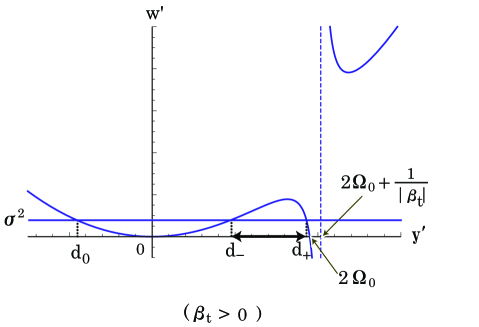
Figure 4: The behavior of the relation (9.15) for $\beta_{t}>0$ is depicted. Here, $\Omega_{0}=19/2$ and $t=5/2$ are adopted which lead to $\beta_{t}=(14-15/\sqrt{57})/19\approx 0.632\ (>0)$.

With the use of the new variables, ${\cal H}$ can be rewritten to

$${\cal H}=\varepsilon(2t-1)-\gamma\cdot i(z^{*}-z)\frac{\Lambda_{t}^{a_{2}}(\frac{\gamma_{t}^{2}}{x})}{\gamma_{t}}\ ,$$ (9.6)

$$\frac{\Lambda_{t}^{a_{2}}\left(\frac{\gamma_{t}^{2}}{x}\right)}{\gamma_{t}}=2\Omega_{0}\left(\frac{\gamma_{t}^{2}-\left(\beta_{t}+\frac{1}{2\Omega_{0}}\right)x}{\gamma_{t}^{2}-\beta_{t}x}\right)\ .$$ (9.7)

The relations (8.1) - (8.3) are reduced to

$$i(z^{*}-z)\frac{\Lambda_{t}^{a_{2}}\left(\frac{\gamma_{t}^{2}}{x}\right)}{\gamma_{t}}=2\kappa\ ,$$ (9.8)

$$i(z^{*}-z)=2v\ ,$$ (9.9)

$$v=\frac{\kappa}{y^{\prime}}\ ,\qquad y^{\prime}=\frac{\Lambda_{t}^{a_{2}}\left(\frac{\gamma_{t}^{2}}{x}\right)}{\gamma_{t}}\ .$$ (9.10)

The function $x=f_{t}(y^{\prime})$ in the present case is given by

$$x=f_{t}(y^{\prime})=\frac{\gamma_{t}^{2}(2\Omega_{0}-y^{\prime})}{\beta_{t}(2\Omega_{0}-y^{\prime})+1}\ .$$ (9.11)

We can treat $u$ in the present case under the same idea as that of the case $\Lambda_{t}^{a_{1}}(x)$. Since $u^{2}=x-v^{2}\geq 0$, we have the following inequality:

$$\frac{\gamma_{t}^{2}}{\beta_{t}}\cdot\frac{y^{\prime}{}^{2}(y^{\prime}-2\Omega_{0})}{y^{\prime}-\left(2\Omega_{0}+\frac{1}{\beta_{t}}\right)}\geq\kappa^{2}\ ,$$ (9.12)

i.e.,

$$w^{\prime}=\left\{\begin{array}[]{ll}\displaystyle+\frac{y^{\prime}{}^{2}(y^{\prime}-2\Omega_{0})}{y^{\prime}-\left(2\Omega_{0}+\frac{1}{|\beta_{t}|}\right)}\geq\sigma^{2}\ ,&\quad(\beta_{t}>0)\\ \displaystyle-\frac{y^{\prime}{}^{2}(y^{\prime}-2\Omega_{0})}{y^{\prime}-\left(2\Omega_{0}-\frac{1}{|\beta_{t}|}\right)}\geq\sigma^{2}\ ,&\quad(\beta_{t}<0)\end{array}\right.$$ (9.15)

$$\sigma=\frac{\sqrt{|\beta_{t}|}}{\gamma_{t}}\kappa\ ,\qquad{\dot{\sigma}}=0\ .$$ (9.16)

The case $\gamma_{t}=0$ appears in $2t-1=2\Omega_{0}$ and, later, we will consider this case. The behavior of the relation (9.15) for $\beta_{t}>0$ is depicted in Fig.4. In Fig.4, we can find out the relation

$$d_{-}\leq y^{\prime}\leq d_{t}\ ,\quad{\rm i.e.,}\quad\frac{1}{2}(d_{+}+d_{-})-\frac{1}{2}(d_{+}-d_{-})\leq y^{\prime}\leq\frac{1}{2}(d_{+}+d_{-})+\frac{1}{2}(d_{+}-d_{-})\ .$$ (9.17)

Therefore, the same idea as that shown in the relation (8.15) for $\alpha_{t}<0$ can be adopted:

$$y^{\prime}=\frac{1}{2}(d_{+}+d_{-})+\frac{1}{2}(d_{+}-d_{-})\cos\psi\ .\qquad(\beta_{t}>0)$$ (9.18a)

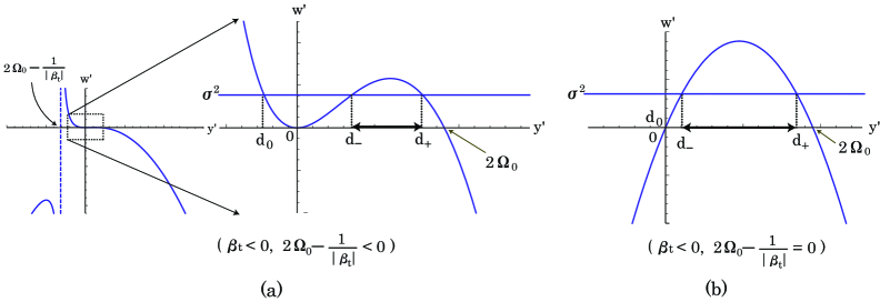
Figure 5: The behavior of the relation (9.15) for $\beta_{t}<0$ is depicted in the case (a) $2\Omega_{0}-1/|\beta_{t}|<0$ and (b) $2\Omega_{0}-1/|\beta_{t}|=0$, separately. Here, in (a), $\Omega_{0}=19/2$ and $t=18/2$ are adopted which lead to $\beta_{t}=(1-6/\sqrt{19})/19\approx-0.0198\ (<0)$ and $2\Omega_{0}-1/|\beta_{t}|\approx-31.466\ (<0)$. In (b), $\Omega_{0}=19/2$ and $t=19/2$ are adopted which lead to $\beta_{t}=-1/19\ (<0)$ and $2\Omega_{0}-1/|\beta_{t}|=0$.

Here, $\psi$ denotes new parameter and, later, the explicit forms of $d_{\pm,0}$ will be shown. In order to treat the $\beta_{t}<0$, some comments are necessary. As was shown in the relations (6.33) and (6.34), the present case $\beta_{t}<0$ appears only in the three cases:

$${\rm(i)}\quad t=\Omega_{0}-\frac{1}{2}\qquad\left(\beta_{\Omega_{0}-1/2}=-\frac{1}{2\Omega_{0}}\left(\frac{1-\frac{1}{\Omega_{0}}}{\sqrt{2-\frac{1}{\Omega_{0}}}+1}\right)\ ,\quad\gamma_{\Omega_{0}-1/2}=\frac{1}{\Omega_{0}}\right)\ ,$$

$${\rm(ii)}\quad t=\Omega_{0}\qquad\left(\beta_{\Omega_{0}}=-\frac{1}{2\Omega_{0}}\ ,\quad\gamma_{\Omega_{0}}=\frac{1}{2\Omega_{0}}\right)\ ,$$

$${\rm(iii)}\quad t=\Omega_{0}+\frac{1}{2}\qquad\left(\beta_{\Omega_{0}+1/2}=-\frac{1}{2\Omega_{0}}\ ,\quad\gamma_{\Omega_{0}+1/2}=0\right)\ .$$

Later, we will contact with the case (iii) separately. The cases (i) and (ii) give us $2\Omega_{0}-1/|\beta_{t}|<0$ and $2\Omega_{0}-1/|\beta_{t}|=0$, respectively. The behavior of the relation (9.15) for $\beta_{t}<0$ is depicted in Fig.5(a) and (b), separately. We can see that the parametrization of the above case is of the same as that shown in the relation (9.18a):

$$y^{\prime}=\frac{1}{2}(d_{+}+d_{-})+\frac{1}{2}(d_{+}-d_{-})\cos\psi\ .\qquad(\beta_{t}<0)$$ (9.18b)

In §10, we will discriminate between the former (9.18a) and the later (9.18b) in terms of the notations $y^{\prime}_{+}$ and $y^{\prime}_{-}$.

By equating both sides of the relation (9.15), we derive the following cubic equation:

$$y^{\prime}{}^{3}-2\Omega_{0}y^{\prime}{}^{2}-\sigma^{2}y^{\prime}+\sigma^{2}\left(2\Omega_{0}+\frac{1}{|\beta_{t}|}\right)=0\ ,\qquad(\beta_{t}>0)$$ (9.19a)

$$-y^{\prime}{}^{3}+2\Omega_{0}y^{\prime}{}^{2}-\sigma^{2}y^{\prime}+\sigma^{2}\left(2\Omega_{0}-\frac{1}{|\beta_{t}|}\right)=0\ .\qquad(\beta_{t}<0)$$ (9.19b)

Three real solutions of Eq.(9.19) give us $d_{\pm,0}$:

$$d_{+}=\frac{2}{3}\left(\Omega_{0}+\sqrt{4\Omega_{0}^{2}+3\sigma^{2}}\cos\frac{\theta}{3}\right)\ ,$$

$$d_{-}=\frac{2}{3}\left(\Omega_{0}-\sqrt{4\Omega_{0}^{2}+3\sigma^{2}}\cos\left(\frac{\theta+\pi}{3}\right)\right)\ ,$$

$$d_{0}=\frac{2}{3}\left(\Omega_{0}-\sqrt{4\Omega_{0}^{2}+3\sigma^{2}}\cos\left(\frac{\theta-\pi}{3}\right)\right)\ ,\qquad(\beta_{t}>0)$$ (9.20a)

$$d_{+}=\frac{2}{3}\left(\Omega_{0}+\sqrt{4\Omega_{0}^{2}-3\sigma^{2}}\cos\frac{\theta}{3}\right)\ ,$$

$$d_{-}=\frac{2}{3}\left(\Omega_{0}-\sqrt{4\Omega_{0}^{2}-3\sigma^{2}}\cos\left(\frac{\theta+\pi}{3}\right)\right)\ ,$$

$$d_{0}=\frac{2}{3}\left(\Omega_{0}-\sqrt{4\Omega_{0}^{2}-3\sigma^{2}}\cos\left(\frac{\theta-\pi}{3}\right)\right)\ .\qquad(\beta_{t}<0)$$ (9.20b)

Here, $\theta$ ($0\leq\theta\leq\pi$) denotes a parameter which satisfies

$$\cos\theta=\frac{8\Omega_{0}^{3}-9\left(\frac{3}{2|\beta_{t}|}+2\Omega_{0}\right)\sigma^{2}}{\left(\sqrt{4\Omega_{0}^{2}+3\sigma^{2}}\right)^{3}}\qquad{\rm for}\quad\beta_{t}>0\ ,$$ (9.21a)

$$\cos\theta=\frac{8\Omega_{0}^{3}-9\left(\frac{3}{2|\beta_{t}|}-2\Omega_{0}\right)\sigma^{2}}{\left(\sqrt{4\Omega_{0}^{2}-3\sigma^{2}}\right)^{3}}\qquad{\rm for}\quad\beta_{t}<0\ .$$ (9.21b)

$$\frac{3}{2|\beta_{t}|}-2\Omega_{0}>0\qquad{\rm for}\quad\beta_{t}<0\ .$$ (9.21c)

The relations (6.33) and (6.34) support the inequality (9.21c). The above three quantities $d_{\pm,0}$ satisfy

$$d_{+}+d_{-}+d_{0}=2\Omega_{0}\ .$$ (9.22)

With the use of the relation (9.20), we have the following expression:

$$\frac{1}{2}(d_{+}+d_{-})=\frac{1}{3}\left(2\Omega_{0}+\sqrt{4\Omega_{0}^{2}+3\sigma^{2}}\cos\left(\frac{\pi-\theta}{3}\right)\right)\ ,$$

$$\frac{1}{2}(d_{+}-d_{-})=\frac{1}{\sqrt{3}}\sqrt{4\Omega_{0}^{2}+3\sigma^{2}}\sin\left(\frac{\pi-\theta}{3}\right)\ ,\qquad(\beta_{t}>0)$$ (9.23a)

$$\frac{1}{2}(d_{+}+d_{-})=\frac{1}{3}\left(2\Omega_{0}+\sqrt{4\Omega_{0}^{2}-3\sigma^{2}}\cos\left(\frac{\pi-\theta}{3}\right)\right)\ ,$$

$$\frac{1}{2}(d_{+}-d_{-})=\frac{1}{\sqrt{3}}\sqrt{4\Omega_{0}^{2}-3\sigma^{2}}\sin\left(\frac{\pi-\theta}{3}\right)\ .\qquad(\beta_{t}<0)$$ (9.23b)

By substituting the above result (9.23) into the relation (9.18), we are able to obtain $y^{\prime}$ as a function of $\cos\psi$.

With the use of $y^{\prime}$, we have the expressions for $x^{\prime}$ and $\Lambda_{t}^{a_{2}}(x^{\prime})$ in the form

$$x^{\prime}=\frac{\gamma_{t}^{2}}{x}=\beta_{t}+\frac{1}{2\Omega_{0}-y^{\prime}}\ ,$$ (9.24)

$$\Lambda_{t}^{a_{2}}(x^{\prime})=\Lambda_{t}^{a_{2}}\left(\frac{\gamma_{t}^{2}}{x}\right)=\gamma_{t}y^{\prime}\ .$$ (9.25)

The relation (9.24) is applicable in the range $\gamma_{t}\leq x^{\prime}<\infty$. In §10, this point will be discussed. In the relation (9.18), $y^{\prime}$ is given as a function of $\cos\psi$. Therefore, if the time-dependence of $\psi$ is determined, we are able to have the time-dependence of $\Lambda_{t}^{a_{2}}(x^{\prime})$. Concerning to this point, we can see that in the case $\gamma_{t}=0$, $\Lambda_{t}^{a_{2}}(x^{\prime})$ vanishes. It is quite natural and the reason is simple: The case $\gamma_{t}=0$ gives us the relation $2t-1=2\Omega_{0}$ and the relations (4.23) and (5.39) suggest us that this case corresponds to the maximum seniority number, that is, there does not exist the possibility of the creation of the Cooper-pair.

Let us investigate the time-dependence of $\psi$. The basic idea is the same as that in the case $\Lambda_{t}^{a_{1}}(x)$. First, we notice that the relation (9.3) can be rewritten as follows:

$${\dot{z}}=\frac{\gamma}{\gamma_{t}}\left[z^{2}-x\left(1-\frac{\Lambda_{t}^{a_{2}}(x^{\prime})}{x^{\prime}\Lambda_{t}^{a_{2}}{}^{\prime}(x^{\prime})}\right)\right]\ ,\quad{\dot{z}}^{*}=\frac{\gamma}{\gamma_{t}}\left[z^{*2}-x\left(1-\frac{\Lambda_{t}^{a_{2}}(x^{\prime})}{x^{\prime}\Lambda_{t}^{a_{2}}{}^{\prime}(x^{\prime})}\right)\right]\ .$$ (9.26)

Here, of course, $x^{\prime}=\gamma_{t}^{2}/x$. Then, we can calculate ${\dot{x}}$:

$${\dot{x}}={\dot{z}}^{*}z+z^{*}{\dot{z}}=2\gamma\cdot\frac{x^{2}}{\gamma_{t}^{3}}\cdot\frac{\Lambda_{t}^{a_{2}}(x^{\prime})}{\Lambda_{t}^{a_{2}}{}^{\prime}(x^{\prime})}\cdot u\ .$$ (9.27)

In a way similar to the case $\Lambda_{t}^{a_{1}}(x)$, $u$ is obtained in the form

$$u=\left\{\begin{array}[]{ll}\displaystyle\pm\frac{\gamma_{t}}{\sqrt{|\beta_{t}|}}\cdot\frac{1}{y^{\prime}}\sqrt{(d_{+}-y^{\prime})(y^{\prime}-d_{-})}\cdot\sqrt{\frac{y^{\prime}-d_{0}}{(2\Omega_{0}+\frac{1}{|\beta_{t}|})-y^{\prime}}}\ ,&\qquad(\beta_{t}>0)\\ \displaystyle\pm\frac{\gamma_{t}}{\sqrt{|\beta_{t}|}}\cdot\frac{1}{y^{\prime}}\sqrt{(d_{+}-y^{\prime})(y^{\prime}-d_{-})}\cdot\sqrt{\frac{y^{\prime}-d_{0}}{y^{\prime}-(2\Omega_{0}-\frac{1}{|\beta_{t}|})}}\ .&\qquad(\beta_{t}<0)\end{array}\right.$$ (9.30)

Here, it is noted that in the case $2\Omega_{0}-1/|\beta_{t}|=0$, $d_{0}=0$ and it corresponds to the situation shown in Fig.5(b). The relations (9.10) and (9.27) lead to the following form for ${\dot{y}}^{\prime}$:

$${\dot{y}}^{\prime}=-\frac{2\gamma}{\gamma_{t}}y^{\prime}\cdot u\ .$$ (9.31)

By substituting the quantity $u$ shown in the relation (9.30), ${\dot{y}}^{\prime}$ is obtained. On the other hand, the result (9.18) gives us

$${\dot{y}}^{\prime}=-\frac{1}{2}(d_{+}-d_{-})\sin\psi\cdot{\dot{\psi}}\ .$$ (9.32)

Equating the expressions (9.31) and (9.32) and treating the double sign $\pm$ in the same idea as that in the case $\Lambda_{t}^{a_{1}}(x)$, we obtain ${\dot{\psi}}$ in the following form:

$${\dot{\psi}}=\left\{\begin{array}[]{ll}\displaystyle\frac{2\gamma}{\sqrt{|\beta_{t}|}}\sqrt{\frac{(\Omega_{0}-\frac{3}{2}d_{0})+\frac{1}{2}(d_{+}-d_{-})\cos\psi}{\frac{1}{|\beta_{t}|}+(\Omega_{0}+\frac{1}{2}d_{0})-\frac{1}{2}(d_{+}-d_{-})\cos\psi}}\ ,&\quad(\beta_{t}>0)\\ \displaystyle\frac{2\gamma}{\sqrt{|\beta_{t}|}}\sqrt{\frac{(\Omega_{0}-\frac{3}{2}d_{0})+\frac{1}{2}(d_{+}-d_{-})\cos\psi}{\frac{1}{|\beta_{t}|}-(\Omega_{0}+\frac{1}{2}d_{0})+\frac{1}{2}(d_{+}-d_{-})\cos\psi}}\ .&\quad(\beta_{t}<0)\end{array}\right.$$ (9.35)

Here, we used the relation (9.22). By solving the differential equation (9.35), we obtain $\psi$ as a function of $\tau$. But, in spite of simple form, the exact solution may be impossible to obtain in analytical form except the following two cases: (1) $d_{+}=d_{-}$ for $\beta_{t}>0$ and $\beta_{t}<0$ and (2) $\Omega_{0}-(3/2)\cdot d_{0}=1/|\beta_{t}|-(\Omega_{0}+d_{0}/2)$. The case (2) corresponds to Fig. 5(b). Therefore, we must search reasonable approximation for the solution.

10 Various properties of $\Lambda_{t}^{a_{2}}(x)$ for describing its time-dependence — procedure for the application —

Let us consider a guide to the approximation for the differential equation (9.35). We start in rewriting this equation:

$$\frac{1}{2}{\cal J}{\dot{\psi}}^{2}+V_{+}(\psi)=E_{+}\ ,\quad V_{+}(\psi)=-\frac{A_{+}+B}{A_{+}-\cos\psi}\ ,\quad E_{+}=-1\ ,\ (\beta_{t}>0)$$ (10.1a)

$$\frac{1}{2}{\cal J}{\dot{\psi}}^{2}+V_{-}(\psi)=E_{-}\ ,\quad V_{-}(\psi)=+\frac{A_{-}-B}{A_{-}+\cos\psi}\ ,\quad E_{-}=+1\ .\ (\beta_{t}<0)\qquad\qquad$$ (10.1b)

Here, ${\cal J}$, $A_{\pm}$ and $B$ are defined as

$${\cal J}=\frac{|\beta_{t}|}{2\gamma^{2}}\ ,\qquad A_{\pm}=\frac{\frac{2}{|\beta_{t}|}\pm(2\Omega_{0}+d_{0})}{d_{+}-d_{-}}\ ,\qquad B=\frac{2\Omega_{0}-3d_{0}}{d_{+}-d_{-}}\ .$$ (10.2a)

With the use of the relation (9.22) and Figs.4 and 5, we can show that $$A_{\pm} B$$ and obey the inequality

$$A_{\pm}>1\ ,\qquad B>1\ ,\qquad A_{-}>B\ .$$ (10.2b)

The expression (10.1) can be regarded as the total energy $E_{\pm}$ with the kinetic energy ${\cal J}{\dot{\psi}}^{2}/2$ and the potential energy $V_{\pm}(\psi)$. With the aid of the inequality (10.2b), we can prove the following relation:

$$V_{\pm}(\psi)<E_{\pm}\ .\quad(-1\leq\cos\psi\leq 1)$$ (10.3)

Therefore, if the angle variable $\psi$ changes continuously in the range $-\infty<\psi<\infty$, the present case can be understood in terms of the rotational motion with the moment of inertia ${\cal J}$ and the periodically changing angular velocity. However, in the present case, $\psi$ does not change continuously, because the original variable $x^{\prime}$ changes in the range $\gamma_{t}\leq x^{\prime}<\infty$ and the other $x$ in the range $0\leq x\leq\gamma_{t}$. The relation (9.24) suggests us that for certain angle denoted as $\psi^{c}$, the variable $\psi$ should obey the condition

$$\cos\psi^{c}\leq\cos\psi\leq 1\ .$$ (10.4)

This means that any result derived from the relation (10.1) in the range $-1\leq\cos\psi\leq\cos\psi^{c}$ is meaningless. This range is treated in relation to the variable $\chi$ discussed in §8. In this sense, the quantity $\cos\psi^{c}$ plays an essential role in our treatment. Including the value of $\cos\psi^{c}$, the detail will be considered in §10. The above mention is illustrated in Fig.6 for the range $-\pi{\stackrel{{\scriptstyle<}}{{\raisebox{-4.30554pt}{$\sim$}}}}\psi{\stackrel{{\scriptstyle<}}{{\raisebox{-4.30554pt}{$\sim$}}}}\pi$. The longitudinal axis represents $v_{\pm}(\psi)$ defined as

$$V_{\pm}(\psi)=(A_{\pm}\pm B)\cdot v_{\pm}(\psi)\ ,$$ (10.5a)

$$v_{\pm}(\psi)=\mp\frac{1}{A_{\pm}\mp\cos\psi}\ ,\qquad v_{\pm}(-\psi)=v_{\pm}(\psi)\ .$$ (10.5b)

Hereafter, we will treat the angle $\psi$ in the range

$$-\pi\leq\psi\leq\pi\ .$$ (10.6)

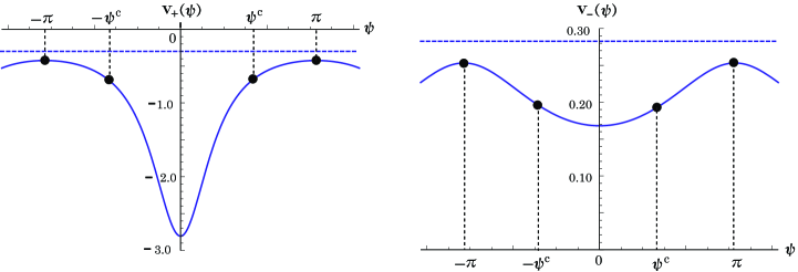
Figure 6: The figure shows $v_{\pm}(\psi)$ as function of $\psi$ in the range $-\pi\leq\psi\leq\pi$. The horizontal dotted line corresponds to $E_{\pm}/(A_{\pm}\pm B)$ $(E_{\pm}=\mp 1)$.

Let us present an idea for the approximation of $v_{\pm}(\psi)$, which will be adopted in this paper. Needless to say, we search a possible approximation in the range

$$-\psi^{c}\leq\psi\leq\psi^{c}\ ,\qquad 0\leq\psi^{c}\leq\pi\ .$$ (10.7)

But, for the time being, forgetting the range (10.7), $\psi$ is treated in the range (10.6). Behavior of $v_{\pm}(\psi)$ is illustrated in Fig.6. In order to understand this behavior more precisely, we take up the first and the second derivative of $v_{\pm}(\psi)$ for $\psi$, $v_{\pm}^{\prime}(\psi)$ and $v^{\prime\prime}_{\pm}(\psi)$:

$$v_{\pm}^{\prime}(\psi)=\frac{\sin\psi}{(A_{\pm}\mp\cos\psi)^{2}}\ ,$$ (10.8a)

$$v_{\pm}^{\prime\prime}(\psi)=\pm\frac{\cos^{2}\psi\pm A_{\pm}\cos\psi-2}{(A_{\pm}\mp\cos\psi)^{3}}\ .$$ (10.8b)

Since $V_{\pm}(\psi)$ represents the potential energy, the force $F_{\pm}(\psi)$ acting on the present system is given in the form

$$F_{\pm}(\psi)=-\frac{dV_{\pm}(\psi)}{d\psi}=-(A_{\pm}\pm B)\cdot v_{\pm}^{\prime}(\psi)\ .$$ (10.9)

Therefore, we can learn characteristics of $F_{\pm}(\psi)$ through $v_{\pm}^{\prime}(\psi)$. Since $F_{\pm}(-\psi)$, i.e., $v_{\pm}^{\prime}(-\psi)=-v_{\pm}^{\prime}(\psi)$, it may be enough to investigate $v_{\pm}^{\prime}(\psi)$ in the range $0\leq\psi\leq\pi$. Its behavior is shown in Fig.7.

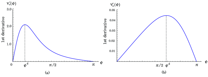
Figure 7: The figure shows $v^{\prime}_{\pm}(\psi)$ as function of $\psi$ in the range $0\leq\psi\leq\pi$.

The angle $\psi^{d}$ gives us the maximum value of $v_{\pm}^{\prime}(\psi)$ and its value is determined by $v_{\pm}^{\prime\prime}(\psi)=0$:

$$\cos\psi^{d}=\pm\frac{1}{2}\left(\sqrt{A_{\pm}^{2}+8}-A_{\pm}\right)\ .$$ (10.10)

The flectional point of $v_{\pm}(\psi)$ is given by $\psi^{d}$ and we have the following:
          (i) $v_{\pm}^{\prime}(\psi)$ is increasing in the range $\psi<\psi^{d}$,
          (ii) $v_{\pm}^{\prime}(\psi)$ is decreasing in the range $\psi>\psi^{d}$.
The above two cases and the relation $F_{\pm}(-\psi)=F_{\pm}(\psi)$ teach us that the force under consideration is attractive for the point, the center of the force and as $|\psi|$ increases, the strength of the force increases in the case (i) and decreases in the case (ii). This indicates that the property of the force is transformed at $\psi=\psi^{d}$. The above is a distinctive feature of $F_{\pm}(\psi)$. With this feature in mind, we consider the approximation of $v_{\pm}(\psi)$ through $v_{\pm}^{\prime}(\psi)$.

In order to obtain the idea, first, we must introduce the angle $\psi^{c}$ into the above argument. In the case $v_{+}^{\prime}(\psi)$, we have two possibilities, which are illustrated in Fig.8. As is clear from the relation (10.7), the force $F_{+}(\psi)$ has its meaning for the solid curve OC. Our idea may be the simplest and it is summarized as follows: (a) In the case (a), the curves OD and DC are replaced with the straight lines OD and DC. (b) In the case (b), the curve OC is replaced with the straight line OC. The above scheme is also applicable to the case $v_{-}^{\prime}(\psi)$. It should be noted that the above approximation preserves the distinctive feature of $F_{\pm}(\psi)$ already mentioned and the values of $v_{\pm}^{\prime}(\psi)$ at $\psi=0$, $\psi^{d}$ and $\psi^{c}$. By adopting the symbol $v_{\pm}^{a}(\psi)$ for the approximate form of $v_{\pm}(\psi)$, the above idea is formulated as follows:

$${\rm(a)} v_{\pm}^{a}{}^{\prime}(\psi)=-w_{\pm}^{cd}\cdot(\psi-\psi^{c})+v_{\pm}^{\prime}(\psi^{c})\ ,\quad\left(w_{\pm}^{cd}=-\frac{v_{\pm}^{\prime}(\psi^{c})-v_{\pm}^{\prime}(\psi^{d})}{\psi^{c}-\psi^{d}}\right)\quad{\rm(DC)}$$ (10.11b)

$$v_{\pm}^{a}{}^{\prime}(\psi)=w_{\pm}^{d}\cdot\psi\ ,\quad\qquad\qquad\qquad\qquad\left(w_{\pm}^{d}=\frac{v_{\pm}^{\prime}(\psi^{d})}{\psi^{d}}\right)\qquad{\rm(OD)}$$

$${\rm(b)}\quad v_{\pm}^{a}{}^{\prime}(\psi)=w_{\pm}^{c}\cdot\psi\ .\quad\left(w_{\pm}^{c}=\frac{v_{\pm}^{\prime}(\psi^{c})}{\psi^{c}}\right)\qquad\qquad\qquad\quad\qquad\quad{\rm(OC)}\qquad$$ (10.12)

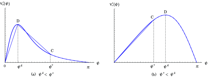
Figure 8: The figure shows $v^{\prime}_{\pm}(\psi)$ as function of $\psi$ in the range $0\leq\psi\leq\pi$. The solid curves and dot-dashed curves represent the exact results. The thin lines represent the approximate ones. (a) The parameters are taken as $\kappa=-15/2$, $t=5/2$ and $\Omega_{0}=19/2$. Here, $\alpha_{t}\approx 0.7656\ (>0)$ and $\beta_{t}\approx 0.6323\ (>0)$ are derived. Also, $A_{+}\approx 1.3564$, $\psi^{c}\approx 1.7123$ and $\psi^{d}\approx 0.4729$ are obtained. (b) The parameters are taken as $\kappa=-1$, $t=18/2$ and $\Omega_{0}=19/2$. In this parameter set, $\alpha_{t}\approx-6.0384\ (<0)$ and $\beta_{t}\approx-0.0198\ (<0)$ are derived. Here, $A_{-}\approx 4.9493$, $\psi^{c}\approx 1.4877$ and $\psi^{d}\approx 1.9558$ are obtained.

Naturally, the relations (10.11) and (10.12) give us

$$v_{\pm}^{a}{}^{\prime}(0)=v_{\pm}^{\prime}(0)\ ,\qquad v_{\pm}^{a}{}^{\prime}(\psi^{d})=v_{\pm}^{\prime}(\psi^{d})\ ,\qquad v_{\pm}^{a}{}^{\prime}(\psi^{c})=v_{\pm}^{\prime}(\psi^{c})\ .$$ (10.13)

By integrating the relations (10.11) and (10.12), we are able to obtain the approximate form of $v_{\pm}(\psi)$, $v_{\pm}^{a}(\psi)$.

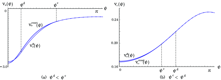
Figure 9: The figure shows $v_{\pm}(\psi)$ as function of $\psi$ in the range $0\leq\psi\leq\pi$. The solid and dot-dashed curves represent the exact results. The thin curves represent the approximate ones. The parameters are the same ones used in Fig.8.

For the integration, we require the condition

$$v_{\pm}^{a}(\psi^{c})=v_{\pm}(\psi^{c})\ .$$ (10.14)

As was already mentioned, the angle $\psi^{c}$ plays a role of the door way to the range treated by $\chi$. Therefore, for obtaining $v_{\pm}^{a}(\psi)$, consideration to the behavior of $v_{\pm}(\psi)$ at $\psi=\pm\psi^{c}$ and the neighbouring region should be prior to any other region. The above consideration suggests us the condition (10.14). By integrating the relation of (LABEL:9-40a) under the condition (10.14), we have the following expression for $v_{\pm}^{a}(\psi)$:

$$v_{\pm}^{a}(\psi)=-\frac{1}{2}w_{\pm}^{cd}\cdot(\psi-\psi^{c})^{2}+v_{\pm}^{\prime}(\psi^{c})\cdot(\psi-\psi^{c})+v_{\pm}(\psi^{c})\ .\ \ {\rm(DC)}$$ (10.15a)

If we require that, at $$\psi=\psi^{d} v_{\pm}^{a}(\psi)$$, the value of from the side OD agrees with that from the side DC for the relation of (10.11b), we obtain the expression

$$v_{\pm}^{a}(\psi)=\frac{1}{2}w_{\pm}^{d}\cdot(\psi^{2}-\psi^{d}{}^{2})-\frac{1}{2}(v_{\pm}^{\prime}(\psi^{c})+v_{\pm}^{\prime}(\psi^{d}))\cdot(\psi^{c}-\psi^{d})+v_{\pm}(\psi^{c})\ .\ {\rm(OD)}$$

(10.15b)

The above requirement may be acceptable, because the present system conserves the energy. For the case (b), the condition (10.12) gives us the following expression:

$$v_{\pm}^{a}(\psi)=\frac{1}{2}w_{\pm}^{c}(\psi^{2}-\psi^{c}{}^{2})+v_{\pm}(\psi^{c})\ .\qquad{\rm(OC)}$$ (10.16)

By replacing $\psi$ with $-\psi$, we have the expressions in the range $-\psi^{c}\leq\psi\leq 0$. Thus, we obtained the approximate expressions of $v_{\pm}(\psi)$ in our scheme. It should be noted that, owing to the approximation, we are forced to have $v_{\pm}^{a}(0)\neq v_{\pm}(0)$, and $v_{\pm}^{a}(\psi^{d})\neq v_{\pm}(\psi^{d})$. In Fig.9, the solid and dot-dashed curves represent the exact $v_{\pm}(\psi)$. Under the idea formulated by (10.11)-(10.13), the approximate $v_{\pm}^{a}(\psi)$ are obtained and are shown by thin curves. Figure 9 shows that the $v_{\pm}^{a}(\psi)$ presents a good approximation for the exact result in the range $-\psi^{c}\leq\psi\leq\psi^{c}$ under consideration.

Finally, we will sketch the approximate solution of $\psi$ as a function of $\tau$. The relation (10.1) leads us to the following approximate expression for ${\dot{\psi}}$:

$${\dot{\psi}}=\sqrt{\frac{2}{\cal J}(E_{\pm}-(A_{\pm}\pm B)v_{\pm}^{a}(\psi))}\ .$$ (10.17)

For $v_{\pm}^{a}(\psi)$, the relations (10.15) and (10.16) must be used. As can be seen in the forms (10.15) and (10.16), the potential energy is expressed as a quadratic function of $\psi$. For the coefficients of $\psi^{2}$, we have the inequalities

$$w_{\pm}^{cd}>0\ ,\qquad w_{\pm}^{d}>0\ ,\qquad w_{\pm}^{c}>0\ .$$ (10.18)

Therefore, $\psi$ can be simply expressed in the form

$$\psi(\tau)=\psi_{h}(\tau)={\cal A}_{h}\sinh(\omega_{h}\tau+\alpha_{h})+{\cal B}_{h}\ ,\qquad{\rm(CD)}$$ (10.19a)

$$\psi(\tau)=\psi_{n}(\tau)={\cal A}_{n}\sin(\omega_{n}\tau+\alpha_{n})+{\cal B}_{n}\ .\qquad\ \ {\rm(OD),\ (OC)}$$ (10.19b)

Then, our problem is reduced to determine the coefficients $({\cal A}_{h},\omega_{h},\alpha_{h},{\cal B}_{h})$ and $({\cal A}_{n},\omega_{n},\alpha_{n},{\cal B}_{n})$. In next section, some examples will be given.

11 Discussion

One of the aims of this paper is to describe a simple many-fermion model obeying the pseudo $su(1,1)$-algebra in terms of the time-dependent variational method. In this description, the function $\Lambda_{t}(x)$ plays a central role. For its original form, we adopted an approximate form which consists of two parts: $\Lambda_{t}^{a_{1}}(x)$ for $0\leq x\leq\gamma_{t}$ and $\Lambda_{t}^{a_{2}}(x^{\prime})$ for $\gamma_{t}\leq x^{\prime}<\infty$. Treating both parts independently in §§8 and 9, we derived various features induced by these two functions. Therefore, it is inevitable to investigate connection between the results derived from two forms. For this aim, it may be convenient to discuss the connection under four categories, although they are correlated with one another.

First is related to constants of motion. We already mentioned that $t$ is one of them, i.e., common to the two parts. The others are $\rho$ in the range $0\leq x\leq\gamma_{t}$ and $\sigma$ in the range $\gamma_{t}\leq x^{\prime}<\infty$ shown in the relations (8.12) and (9.16), respectively. They are not independent to each other. By eliminating $\kappa$ in both relations, we have

$$\sigma=\frac{1}{\gamma_{t}}\sqrt{\frac{|\beta_{t}|}{|\alpha_{t}|}}\cdot\rho\ ,\quad{\rm i.e.,}\quad\sigma^{2}=\frac{1}{\gamma_{t}^{2}}\cdot\frac{|\beta_{t}|}{|\alpha_{t}|}\cdot\rho^{2}\ .$$ (11.1a)

As is clear from Figs.3(b), 4 and 5, $$\rho^{2} \sigma^{2} \rho^{2} \infty \sigma^{2} \beta_{t}>0 \sigma^{2} (\sigma^{2})_{\rm max}$$ and have the maximum values. On the other hand, Fig.3(a) shows that in this case, formally, is permitted to become . But, the relation (11.1) teaches us that in this case, also, there exists the maximum value, because has the maximum value. For example, in the case , the maximum value of , , is given by

$$(\sigma^{2})_{\rm max}=\frac{d_{m}^{2}(d_{m}-2\Omega_{0})}{d_{m}-\left(2\Omega_{0}+\frac{1}{\beta_{t}}\right)}\ ,\qquad d_{m}=2\Omega_{0}\left(1-\frac{2}{3+\sqrt{9+16\Omega_{0}|\beta_{t}|}}\right)\ .$$ (11.1b)

Here, $d_{m}$ denotes the value of $y^{\prime}$ which makes $w^{\prime}$ in the relation (9.15) the maximum.

The ranges covered by $x$ and $x^{\prime}$ are $0\leq x\leq\gamma_{t}$ and $\gamma_{t}\leq x^{\prime}<\infty$, respectively. Second is related to these ranges. The relation (8.7) and (9.24) lead to the following inequalities:

$$0\leq\frac{1}{\alpha_{t}}\left(1-\frac{2t}{y}\right)\leq\gamma_{t}\ ,$$ (11.2a)

$$\gamma_{t}\leq\beta_{t}+\frac{1}{2\Omega_{0}-y^{\prime}}<\infty\ .$$ (11.2b)

The inequality (11.2a) gives us

$$2t\leq y_{+}\leq 2\Omega_{0}\left(1-\frac{1}{1+\sqrt{2t\gamma_{t}}}\right)\ ,$$ (11.3)

$$2\Omega_{0}\left(1-\frac{1}{1+\sqrt{2t\gamma_{t}}}\right)\leq y_{-}\leq 2t\ .$$ (11.4)

Also, the inequality (11.2b) gives us

$$2\Omega_{0}\left(1-\frac{1}{1+\sqrt{2t\gamma_{t}}}\right)\leq y_{\pm}^{\prime}\leq 2t\ .$$ (11.5)

For the derivation of the inequalities (11.4) and (11.5), we used the relation (6.14). It should be noted that although $y_{+}$ contains $\cosh\chi$, it should be finite.

At the point $x=x^{\prime}=\gamma_{t}$, $y$ connects to $y^{\prime}$. As was shown in the relations (8.15) and (9.18), $y$ and $y^{\prime}$ consist of $y_{\pm}$ and $y_{\pm}^{\prime}$, respectively. Therefore, it is necessary to investigate, for example, if $y_{+}$ can connect to $y^{\prime}$ or not. Third is concerned with the above. Formally, we can find four combinations between $y$ and $y^{\prime}$: $(y_{+},y_{+}^{\prime})$, $(y_{+},y^{\prime}_{-})$, $(y_{-},y^{\prime}_{+})$ and $(y_{-},y^{\prime}_{-})$. The relations from (6.26) to (6.35) with the interpretations for them lead us to the following three cases:

$${\rm(i)}\quad{\rm if}\quad\frac{1}{2}\leq t<t^{0}\ ,\qquad 0<\alpha_{t}\leq\beta_{t}\ ,\quad({\rm in\ the\ case}\ t=1/2\ ,\alpha_{t}=\beta_{t})$$ (11.6a)

$${\rm(ii)}\quad{\rm if}\quad t^{0}<t<t^{0}{}^{\prime}\ ,\qquad\alpha_{t}<0<\beta_{t}\ ,$$ (11.6b)

$${\rm(iii)}\quad{\rm if}\quad t^{0}{}^{\prime}<t\leq\Omega_{0}+\frac{1}{2}\ ,\qquad\alpha_{t}<\beta_{t}<0\ .$$ (11.6c)

If the relation $\alpha_{t}<\beta_{t}$ is noticed, the above three cases may be understandable. The cases (i), (ii) and (iii) correspond to the combinations $(y_{+},y^{\prime}_{+})$, $(y_{-},y_{+}^{\prime})$ and $(y_{-},y_{-}^{\prime})$, respectively. Therefore, $y_{+}$ cannot connect with $y_{-}^{\prime}$.

For the above three combinations, we show the maximum values of the squares of the constants of motion $\kappa^{2}$ introduced in the relation (8.1). The conditions $c_{+}-c_{-}=0$ and $d_{+}-d_{-}=0$ give us the maximum values $\kappa_{m}^{(i)2}$ $(i=1,2,3,4)$ for the cases (1), (2), (3) and (4) related to Figs.3(a), 3(b), 4 and 5, respectively. With the use of these conditions, we obtain the following results:

$${\rm(1)}\quad\kappa_{m}^{(1)}{}^{2}\rightarrow\infty\ ,\qquad(y_{+};\ {\rm Fig.3(a)})$$ (11.7a)

$${\rm(2)}\quad\kappa_{m}^{(2)}{}^{2}=\frac{t^{2}}{|\alpha_{t}|}\ ,\qquad(y_{-};\ {\rm Fig.3(b)})$$ (11.7b)

$${\rm(3)}\quad\kappa_{m}^{(3)}{}^{2}=\frac{\gamma_{t}^{2}}{|\beta_{t}|}\cdot\frac{16\Omega_{0}^{3}}{9(4\Omega_{0}+\frac{3}{|\beta_{t}|})}\ ,\qquad(y_{+}^{\prime};\ {\rm Fig.4})$$ (11.7c)

$${\rm(4)}\quad\kappa_{m}^{(4)}{}^{2}=\frac{\gamma_{t}^{2}}{|\beta_{t}|}\cdot\frac{4\Omega_{0}^{2}}{3}\ .\qquad(y_{-}^{\prime};\ {\rm Fig.5})$$ (11.7d)

For the combination $(y_{+},y_{+}^{\prime})$, we choose the smaller value of $\kappa_{m}^{2}$, i.e., $\kappa_{m}^{(3)2}$. For the combination $(y_{-},y_{+}^{\prime})$ and $(y_{-},y_{-}^{\prime})$, we choose the smaller values of $\kappa_{m}^{2}$ for each case; ${\rm min}\{\kappa_{m}^{(2)2},\kappa_{m}^{(3)2}\}$ and ${\rm min}\{\kappa_{m}^{(2)2},\kappa_{m}^{(4)2}\}$, respectively.

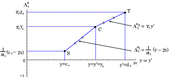
Figure 10: The path of the evolution is illustrated in the case of $\Omega_{0}=19/2$ and $t=5/2$.

Forth is related to giving the explicit expression of the connection. First, let us notice again that $\Lambda_{t}^{a_{1}}(x)$ and $\Lambda_{t}^{a_{2}}(x^{\prime})$ should connect with each other smoothly at $x=x^{\prime}=\gamma_{t}$:

$$\Lambda_{t}^{a_{1}}(\gamma_{t})=\Lambda_{t}^{a_{2}}(\gamma_{t})\ ,\qquad\Lambda_{t}^{a_{1}}{}^{\prime}(\gamma_{t})=\Lambda_{t}^{a_{2}}{}^{\prime}(\gamma_{t})\ .$$ (11.8)

The explicit expression of the relation (11.8) are presented in the relation (6.13). The first of the relation (11.8) and the definition of $y$ and $y^{\prime}$ in (8.3) and (9.10) lead to

$$(y)_{t}=(y^{\prime})_{t}\ (=y_{t})\ .$$ (11.9)

Here, $(y)_{t}$ and $(y^{\prime})_{t}$ denote the values of $y$ and $y^{\prime}$ at the point $x=x^{\prime}=\gamma_{t}$, respectively and, with the use of the relation (6.14), $y_{t}$ is given by

$$y_{t}=2\Omega_{0}\left(1-\frac{1}{1+\sqrt{2t\gamma_{t}}}\right)\ .$$ (11.10)

The above is the connection between the results derived from the two forms.

Our final task is to investigate the time-evolution of $\Lambda_{t}$ in the approximate form, $\Lambda_{t}^{a}$. The path of the evolution is illustrated in Fig.10. The lines SC and CT correspond to $\Lambda_{t}^{a_{1}}=(y-2t)/\alpha_{t}$ and $\Lambda_{t}^{a_{2}}=\gamma_{t}y^{\prime}$, respectively. Here, $y$ and $y^{\prime}$ are given in the relations (8.15) and (9.18), respectively. They depend on two constants of motion, $t$ and $\kappa$. It is noted that $\Lambda_{t}^{a}$ has the minimum and the maximum values which correspond to $y=c_{+}$ and $y^{\prime}=d_{+}$, respectively. At the point C, $\Lambda_{t}^{a}$ changes from $\Lambda_{t}^{a_{1}}$ to $\Lambda_{t}^{a_{2}}$, i.e., from $y$ to $y^{\prime}$ and vice versa. The dependence of $\Lambda_{t}^{a}$ on the time $\tau$ may be periodic. One cycle consists of four paths (S$\rightarrow$C, C$\rightarrow$T, T$\rightarrow$C, C$\rightarrow$S), which is shown in Fig.10.

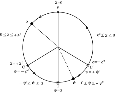
Figure 11: The values of $\chi$ and $\psi$ on each point are shown.

With the use of the relation (11.9) with (8.15) and (9.18), we have the following relations:

$$\cosh\chi^{c}=\frac{y_{t}-\frac{1}{2}(c_{+}+c_{-})}{\frac{1}{2}(c_{+}-c_{-})}\quad(\alpha_{t}>0)\ ,\qquad\cos\chi^{c}=\frac{y_{t}-\frac{1}{2}(c_{+}+c_{-})}{\frac{1}{2}(c_{+}-c_{-})}\quad(\alpha_{t}<0)\ ,$$

(11.11)

$$\cos\psi^{c}=\frac{y_{t}-\frac{1}{2}(d_{+}+d_{-})}{\frac{1}{2}(d_{+}-d_{-})}\quad(\beta_{t}>0\ ,\ \beta_{t}<0)\ .$$ (11.12)

Here, $\chi^{c}$ and $\psi^{c}$ denote the values of $\chi$ and $\psi$ at the point C, respectively. It is noticed that if $\chi^{c}$ and $\psi^{c}$ are positive, $-\chi^{c}$ and $-\psi^{c}$ also satisfy the relations (11.11) and (11.12), respectively. The angle $\psi^{c}$ is nothing but that introduced in §9. On the other hand, $\chi$ and $\psi$ are equal to 0 at the point S and the point T, respectively. The above consideration permits us to choose $\chi$ and $\psi$ including the signs of $\chi^{c}$ and $\psi^{c}$ in the form shown in Fig.11. For the cycle (S$\rightarrow$C$\rightarrow$T$\rightarrow$C’(=C)$\rightarrow$S), it may be enough to regard ${\dot{\chi}}$ and ${\dot{\psi}}$ as positive, ${\dot{\chi}}>0$ and ${\dot{\psi}}>0$, at any position except the point S with ${\dot{\chi}}=0$ and the point T with ${\dot{\psi}}=0$. It is easily verified by $\sinh\chi=\sin\chi=\sin\psi=0$ for $\chi=\psi=0$. The time derivatives ${\dot{\chi}}$ and ${\dot{\psi}}$ are given in the relations (8.43) and (10.17), respectively. We already mentioned that there are three cases for the combinations at the point C: $(y_{+},y^{\prime}_{+})$, $(y_{+},y^{\prime}_{-})$ and $(y_{-},y^{\prime}_{-})$. If applying this rule to the present cycle, we obtain the following three cases:

$${\rm(i)}\ \ \ \alpha_{t}>0\quad({\rm S}\rightarrow{\rm C})\ ,\qquad\beta_{t}>0\quad({\rm C}\rightarrow{\rm T}\rightarrow{\rm C^{\prime}(=C)})\ ,\qquad\alpha_{t}>0\quad({\rm C^{\prime}}\rightarrow{\rm S})\ ,$$

$${\rm(ii)}\ \ \alpha_{t}>0\quad({\rm S}\rightarrow{\rm C})\ ,\qquad\beta_{t}<0\quad({\rm C}\rightarrow{\rm T}\rightarrow{\rm C^{\prime}(=C)})\ ,\qquad\alpha_{t}>0\quad({\rm C^{\prime}}\rightarrow{\rm S})\ ,$$

$${\rm(iii)}\ \alpha_{t}<0\quad({\rm S}\rightarrow{\rm C})\ ,\qquad\beta_{t}<0\quad({\rm C}\rightarrow{\rm T}\rightarrow{\rm C^{\prime}(=C)})\ ,\qquad\alpha_{t}<0\quad({\rm C^{\prime}}\rightarrow{\rm S})\ .$$

We take up the case where the cycle starts from the point S, that is, the initial condition is given by $\chi^{0}=0$ at $\tau^{0}=0$. Here, $\chi^{0}$ and $\tau^{0}$ appear in the relation (8.43). In order to demonstrate our idea, we present several results derived in the case (i) with $\psi^{c}>\psi^{d}$. In this case, there exists the flectional point D specified by $\psi=\pm\psi^{d}$ between C and T and also between T and C’. Then, the path (C$\rightarrow$T$\rightarrow$C’(=C)) is decomposed into the three: C$\rightarrow$D, D$\rightarrow$T and T$\rightarrow$D’(=D). We discriminate between D and D’ by the condition ($\psi_{D}=-\psi^{d}$, $\psi_{D^{\prime}}=\psi^{d}$). General solutions of the paths (S$\rightarrow$C, C’$\rightarrow$S), (C$\rightarrow$D, D’$\rightarrow$C’) and (D$\rightarrow$T, T$\rightarrow$D’) are given by the relations (8.43), (10.19a) and (10.19b), respectively. The parameters $(\omega_{h},{\cal A}_{h})$ and $(\omega_{n},{\cal A}_{n})$ contained in the relation (10.19) are obtained in the form

$$\omega_{h}=\sqrt{\frac{A_{+}+B}{\cal J}\cdot w_{+}^{cd}}\ ,$$ (11.13a)

$${\cal A}_{h}=\sqrt{\frac{2}{w_{+}^{cd}}\left(\frac{E_{+}}{A_{+}+B}-v_{+}(\psi^{c})\right)-\left(\frac{v_{+}^{\prime}(\psi^{c})}{w_{+}^{cd}}\right)^{2}}\ ,\qquad\qquad\qquad\qquad\qquad\qquad$$ (11.13b)

$$\omega_{n}=\sqrt{\frac{A_{+}+B}{\cal J}\cdot w_{+}^{d}}\ ,$$ (11.14a)

$${\cal A}_{n}=\sqrt{\frac{2}{w_{+}^{d}}\left(\frac{E_{+}}{A_{+}+B}-v_{+}(\psi^{c})\right)+{\psi^{d}}^{2}+\frac{1}{w_{+}^{d}}\left(v_{+}^{\prime}(\psi^{c})+v_{+}^{\prime}(\psi^{d})\right)\left(\psi^{c}-\psi^{d}\right)}\ .$$

(11.14b)

Here, we used the relation (10.11) or (10.1a) with $V_{+}(\psi)=(A_{+}+B)v_{+}^{a}(\psi)$. The other parameters $(\alpha_{h},{\cal B}_{h})$ and $(\alpha_{n},{\cal B}_{n})$ can be determined through the conditions governing each path.

Let $\tau^{C}$, $\tau^{D}$, $\tau^{T}$, $\tau^{D^{\prime}}$, $\tau^{C^{\prime}}$ and $\tau^{S}$ denote the arrival, i.e., departure times at the points C, D, T, D’, C’ and S, respectively, after the cycle starts from S at the time $\tau^{0}=0$. Then, these times obey the following condition:

$$\begin{array}[]{ll}(1)\ \chi(0)=0\ ,\quad\chi(\tau^{C})=\chi^{c}\ ,&(2)\ \psi_{h}(\tau^{C})=-\psi^{c}\ ,\quad\psi_{h}(\tau^{D})=-\psi^{d}\ ,\\ (3)\ \psi_{n}(\tau^{D})=-\psi^{d}\ ,\quad\psi_{n}(\tau^{T})=0\ ,&(4)\ \psi_{n}(\tau^{T})=0\ ,\quad\psi_{n}(\tau^{D^{\prime}})=\psi^{d}\ ,\\ (5)\ \psi_{h}(\tau^{D^{\prime}})=\psi^{d}\ ,\quad\psi_{h}(\tau^{C^{\prime}})=\psi^{c}\ ,&(6)\ \chi(\tau^{C^{\prime}})=-\chi^{c}\ ,\quad\chi(\tau^{S})=0\ .\end{array}$$ (11.18)

Under the condition (11.18), we can determine $(\alpha_{h},{\cal B}_{h})$ and $(\alpha_{n},{\cal B}_{n})$ and $\chi(\tau)$ and $\psi(\tau)$ for each path are given in the following form:

$$(1)\ {\rm S}\rightarrow{\rm C}\ ;\ \chi(\tau)=2\gamma\sqrt{|\alpha_{t}|}\cdot\tau\ ,\quad(0\leq\tau\leq\tau^{C})$$ (11.19a)

$$(2)\ {\rm C}\rightarrow{\rm D}\ ;\ \psi(\tau)={\cal A}_{h}\sinh\left[\omega_{h}(\tau-\tau^{C})+\sinh^{-1}\left(\frac{v_{+}^{\prime}(\psi^{c})}{{\cal A}_{h}w_{+}^{cd}}\right)\right]-\frac{v_{+}^{\prime}(\psi^{c})}{w_{+}^{cd}}-\psi^{c}\ ,$$

$$\qquad\qquad\qquad\qquad\qquad\qquad\qquad\qquad\qquad\qquad\qquad\qquad(\tau^{C}\leq\tau\leq\tau^{D})$$ (11.19b)

$$(3)\ {\rm D}\rightarrow{\rm T}\ ;\ \psi(\tau)={\cal A}_{n}\sin\left[\omega_{n}(\tau-\tau^{D})-\sin^{-1}\left(\frac{\psi^{d}}{{\cal A}_{n}}\right)\right]\ ,\quad(\tau^{D}\leq\tau\leq\tau^{T})$$ (11.19c)

$$(4)\ {\rm T}\rightarrow{\rm D^{\prime}}\ ;\ \psi(\tau)={\cal A}_{n}\sin\left[\omega_{n}(\tau-\tau^{T})\right]\ ,\quad(\tau^{T}\leq\tau\leq\tau^{D^{\prime}})$$ (11.19d)

$$(5)\ {\rm D^{\prime}}\rightarrow{\rm C^{\prime}}\ ;\ \psi(\tau)={\cal A}_{h}\sinh\left[\omega_{h}(\tau-\tau^{D^{\prime}})-\sinh^{-1}\left(\frac{1}{{\cal A}_{h}}\left(\psi^{c}-\psi^{d}+\frac{v_{+}^{\prime}(\psi^{c})}{w_{+}^{cd}}\right)\right)\right]$$

$$\qquad\qquad\qquad\qquad\qquad+\left(\psi^{c}-\psi^{d}+\frac{v_{+}^{\prime}(\psi^{c})}{w_{+}^{cd}}\right)+\psi^{d}\ ,\quad(\tau^{D^{\prime}}\leq\tau\leq\tau^{C^{\prime}})$$ (11.19e)

$$(6)\ {\rm C^{\prime}}\rightarrow{\rm S}\ ;\ \chi(\tau)=2\gamma\sqrt{|\alpha_{t}|}\cdot(\tau-\tau^{C^{\prime}})-\chi^{c}\ .\quad(\tau^{C^{\prime}}\leq\tau\leq\tau^{S})$$ (11.19f)

In connection to the relations (7.21) and (7.22), it was suggested that our model enables us to describe the dissipation phenomena in many-fermion system. The paths (1) and (6) correspond to this suggestion. It indicates that this dissipation cannot be observed at any time. The condition (11.18) also gives us the time intervals for the paths:

$$\tau^{S}-\tau^{C^{\prime}} = \tau^{C}=\frac{\chi^{c}}{2\gamma\sqrt{|\alpha_{t}|}}\ ,$$ (11.20a)

$$\tau^{C^{\prime}}-\tau^{D^{\prime}} = \tau^{D}-\tau^{C}$$ (11.20b)

$$= \frac{1}{\omega_{h}}\left\{\sinh^{-1}\left[\frac{1}{{\cal A}_{h}}\left(\psi^{c}-\psi^{d}+\frac{v^{\prime}_{+}(\psi^{c})}{w_{+}^{cd}}\right)\right]-\sinh^{-1}\left(\frac{v^{\prime}_{+}(\psi^{c})}{{\cal A}_{h}w_{+}^{cd}}\right)\right\}\ ,\quad$$

$$\tau^{D^{\prime}}-\tau^{T} = \tau^{T}-\tau^{D}$$ (11.20c)

$$= \frac{1}{\omega_{n}}\sin^{-1}\left(\frac{\psi^{d}}{{\cal A}_{n}}\right)\ .$$

The results (11.20a)$\sim$(11.20c) give us $\tau^{C}$ etc. For example, we have

$$\tau^{S}=2\tau^{T}\ ,$$ (11.21a)

$$\tau^{T}=\frac{\chi^{c}}{2\gamma\sqrt{|\alpha_{t}|}}+\frac{1}{\omega_{h}}\left\{\sinh^{-1}\left[\frac{1}{{\cal A}_{h}}\left(\psi^{c}-\psi^{d}+\frac{v^{\prime}_{+}(\psi^{c})}{w_{+}^{cd}}\right)\right]-\sinh^{-1}\left(\frac{v^{\prime}_{+}(\psi^{c})}{{\cal A}_{h}w_{+}^{cd}}\right)\right\}$$

$$\qquad\qquad+\frac{1}{\omega_{n}}\sin^{-1}\left(\frac{\psi^{d}}{{\cal A}_{n}}\right)\ .$$ (11.21b)

The time $\tau^{S}$ is nothing but the period of the cycle. Figure 12 illustrates how $\chi(\tau)$ and $\psi(\tau)$ behave in one cycle.

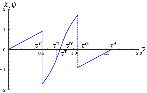
Figure 12: It is illustrated how $\chi(\tau)$ and $\psi(\tau)$ behave in one cycle. Here, the same parameters as those used in Fig.8 (a) are adopted.

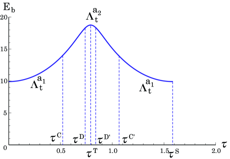
Figure 13: The approximate energy of the intrinsic system, $\langle{\widetilde{H}}_{\overline{P}}\rangle=\varepsilon N_{\overline{P}}$, is shown as a function of time $\tau$ under the same parameter set as those used in Fig.8 (a).

Here, in the regions of $\tau\leq\tau^{C}$ and $\tau\geq\tau^{C^{\prime}}$, $\chi(\tau)$ is shown and is a linear function with respect to time $\tau$. In the region of $\tau^{C}\leq\tau\leq\tau^{C^{\prime}}$, $\psi(\tau)$ is used, and from $\tau^{C}$ to $\tau^{T}$, $\psi(\tau)$ is changed from $\sinh$-type to $\sin$-type function and vice versa from $\tau^{T}$ to $\tau^{C^{\prime}}$. Our main interest is concerned with the energy of the intrinsic system expressed in the form

$$E_{b}\equiv({\phi}|{\widetilde{H}}_{\overline{P}}|{\phi})=\varepsilon N_{\overline{P}}\ .$$ (11.22)

Here, ${\widetilde{H}}_{\overline{P}}$ and $N_{\overline{P}}$ are given in the relations (7.11) and (7.25), respectively and, therefore, it may be enough for the understanding of $E_{b}$ to consider $N_{\overline{P}}$ ($\varepsilon=1$). In Fig.13, the result is shown as a function of $\tau$ under the approximation developed in §§8 - 10 with the same parameters as those used in Fig.8 (a). In the region of $\tau\leq\tau^{C}$ and $\tau\geq\tau^{C^{\prime}}$, $x\leq\gamma_{t}$ is satisfied where $\Lambda_{t}^{a_{1}}(x)$ is used as the approximation of $\Lambda_{t}(x)$. In the region of $\tau^{C}\leq\tau\leq\tau^{C^{\prime}}$, $\Lambda_{t}^{a_{2}}(x)$ is used in the approximation of $\Lambda_{t}(x)$. It is seen that, in one cycle, the energy flows into the intrinsic system from external environment from the time 0 to $\tau^{T}$ and vice versa from $\tau^{T}$ to $\tau^{S}$.

We will discuss some problems related to the result shown in Fig.13. The energy $E_{b}$ shows periodical behavior for time $\tau$. Such behavior cannot be expected in the $su(1,1)$-algebraic model, in which, following the cosh-type change, $E_{b}$ increases or decreases. Since our model belongs to the $su(2)$-algebraic model, the periodical behavior appears. In Fig.13, we can see that there exist the minimum and the maximum value in $E_{b}$. We consider these two values for the case $(\alpha_{t}>0,\beta_{t}>0)$ in a rather general form. The relation (8.15a) teaches us that if $\chi=0$, $y$ becomes the minimum, i.e., $y_{\rm min}=c_{+}$. Then, with the aid of the expression (8.7), we have

$$\left(\Lambda_{t}^{a_{1}}\right)_{\rm min}=\frac{1}{\alpha_{t}}(y_{\rm min}-2t)=\frac{1}{\alpha_{t}}(c_{+}-2t)=\frac{\rho^{2}}{\alpha_{t}}\cdot\frac{1}{t+\sqrt{t^{2}+\rho^{2}}}\ .$$ (11.23)

On the other hand, the relation (9.18a) gives us the maximum value of $y^{\prime}$, if $\psi=0$, i.e., $y^{\prime}_{\rm max}=d_{+}$. Then, the relation (9.25) gives us

$$\left(\Lambda_{t}^{a_{2}}\right)_{\rm max}=\gamma_{t}y^{\prime}_{\rm max}=\gamma_{t}d_{+}\ .$$ (11.24)

Of course, $d_{+}$ is a solution of the cubic equation (9.19a) and we use a possible approximate solution :

$$d_{+}=2\Omega_{0}\left(1-\frac{\sigma^{2}}{2\Omega_{0}|\beta_{t}|}\cdot\frac{2}{4\Omega_{0}^{2}-\sigma^{2}+\sqrt{(4\Omega_{0}^{2}-\sigma^{2})^{2}-\frac{4\sigma^{2}(2\Omega_{0}+d_{m})}{|\beta_{t}|}}}\right)\ .$$ (11.25)

Here, $d_{m}$ is given in the relation (11.1b). In the cases $\sigma^{2}=0$ and $(\sigma^{2})_{\rm max}$, the solution (11.25) is exact. With the aid of the relation (7.25a), $(E_{b})_{\rm min}$ and $(E_{b})_{\rm max}$ are expressed as follows:

$$(E_{b})_{\rm min}=2t-1+\frac{\rho^{2}}{\alpha_{t}}\cdot\frac{1}{t+\sqrt{t^{2}+\rho^{2}}}\ ,$$ (11.26a)

$$(E_{b})_{\rm max}=2\Omega_{0}-\frac{\sigma^{2}}{|\beta_{t}|}\cdot\frac{2\gamma_{t}}{4\Omega_{0}^{2}-\sigma^{2}+\sqrt{(4\Omega_{0}^{2}-\sigma^{2})^{2}-\frac{4\sigma^{2}(2\Omega_{0}+d_{m})}{|\beta_{t}|}}}\ .$$ (11.26b)

In the case $\rho^{2}=0$, $(E_{b})_{\rm min}=2t-1$ and as $\rho^{2}$ increases, $(E_{b})_{\rm min}$ increases. Inversely, in the case $\sigma^{2}=0$, $(E_{b})_{\rm max}=2\Omega_{0}$ and as $\sigma^{2}$ increases, $(E_{b})_{\rm max}$ decreases. For the case $(2\Omega_{0}=19,\ 2t=5,\ 2\kappa=-15)$, we have $(E_{b})_{\rm min}=9.9072$ and $(E_{b})_{\rm max}=18.7569$, which is very near to $(E_{b})_{\rm max}=18.7562$ calculated under the exact solution of the cubic equation (9.19a). This result may support the validity of the approximate form (11.25).

Next, on the basis of the above argument, we investigate the trial state (5.3) which leads us to $(E_{b})_{\rm min}$ and $(E_{b})_{\rm max}$. In the ranges $0\leq x\leq\gamma_{t}$ and $\gamma_{t}\leq x^{\prime}<\infty$, the state (5.3) contains the parameters $z\ (x=|z|^{2})$ and $z^{\prime}\ (x^{\prime}=|z^{\prime}|^{2})$, respectively. Here, the relation (9.1) should be noted. In the range $0\leq x\leq\gamma_{t}$, we note the relation (8.29a) and, then, the value of $x$ at $\chi=0$ is the minimum:

$$x_{\rm min}=\frac{1}{\alpha_{t}}\cdot\frac{\sqrt{t^{2}+\rho^{2}}-t}{\sqrt{t^{2}+\rho^{2}}+t}\ (=x_{\rm min}(\rho^{2}))\ .$$ (11.27)

The function $x_{\rm min}(\rho^{2})$ is increasing for $\rho^{2}$ with $x_{\rm min}(\rho^{2}=0)=0$, i.e., $z=0$. Therefore, the state $|{\phi})$ corresponding to $z=0$ is the minimum weight state (4.15), $|{m_{0}})$, which contains $(2t-1)$ fermions only in ${\overline{P}}\ (N_{\overline{P}}=2t-1,\ N_{P}=0)$. In the range $\gamma_{t}\leq x^{\prime}<\infty$, we note the relation (9.24) and the value of $x^{\prime}$ at $\psi=0$ is the maximum:

$$x^{\prime}_{\rm max} = |\beta_{t}|+\frac{1}{2\Omega_{0}-y^{\prime}_{\rm max}}=|\beta_{t}|+\frac{1}{2\Omega_{0}-d_{+}}$$ (11.28)

$$= \frac{|\beta_{t}|}{\sigma^{2}}\left(4\Omega_{0}^{2}+\sqrt{(4\Omega_{0}^{2}-\sigma^{2})^{2}-\frac{4\sigma^{2}(2\Omega_{0}+d_{m})}{|\beta_{t}|}}\right)\ (=x^{\prime}_{\rm max}(\sigma^{2}))\ .$$

Here, we used the approximate expression (11.25) for $d_{+}$. The function $x^{\prime}_{\rm max}(\sigma^{2})$ is decreasing for $\sigma^{2}$ with $x^{\prime}_{\rm max}(\sigma^{2}=0)\rightarrow\infty$, i.e., $z^{\prime}\rightarrow\infty$. Therefore, the state $|{\phi})$ corresponding to $z^{\prime}\rightarrow\infty$ is $\left({\widetilde{\cal T}}_{+}\right)^{2\Omega_{0}-(2t-1)}|{m_{0}})\ (2s=2\Omega_{0}-(2t-1))$ which contains the maximum number of fermion permitted by the seniority coupling scheme ($N_{\overline{P}}=2\Omega_{0},\ N_{P}=2\Omega_{0}-(2t-1)$). From the above argument, it may be clear that as $\kappa^{2}$ increases from $\kappa^{2}=0$, $\rho^{2}$ and $\sigma^{2}$ also increase from $\rho^{2}=\sigma^{2}=0$ and $(E_{b})_{\rm min}$ and $(E_{b})_{\rm max}$ become larger than $(2t-1)$ and smaller than $2\Omega_{0}$, respectively. If at $\tau=0$, the cycle starts in the point S with $(E_{b})_{\rm min}$, it passes the critical points C and D and at $\tau=\tau^{T}$ arrives at T. Although the points C and D are introduced under the approximation adopted in this paper, they play an essential role for treating the present model in a well-known simple mathematical form.

The above is a basic part which our simple many-fermion model produces under the pseudo $su(1,1)$-algebra.

12 Concluding remarks

In this section, we will give some remarks on the Hamiltonian (7.10). This Hamiltonian was set up under the correspondences (7.7)-(7.9). The original boson Hamiltonian (7.5) is a generator for time-evolution and does not represent the energy of the entire system. It aims at the description of the “damped and amplified harmonic oscillator”. By regarding the mixed-mode boson coherent state as a statistically mixed state, we can describe the harmonic oscillator at finite temperature, which will be shown in the relation (12.6). In this sense, the above-mentioned description provides us a possible entrance to the problems related to finite temperature. The Hamiltonian (7.10) can be regarded as the fermion version of the harmonic oscillator in the $su(1,1)$-algebra in the Schwinger boson representation. Nevertheless, it may be possible to treat the Hamiltonian (7.10) as the energy of the entire system. It was already mentioned in §7. In order to confirm this conjecture, we reexamine the correspondences (7.7)-(7.9).

Let us start in the relation (7.9). The frequency $\omega$ is positive, but, the single-particle energy $\varepsilon$ is not always positive. Therefore, instead of the relation (7.11), it is permissible to set up the following form:

$${\widetilde{H}}_{\overline{P}}=\varepsilon\sum_{\alpha}{\tilde{c}}_{\bar{\alpha}}^{*}{\tilde{c}}_{\bar{\alpha}}\ ,\qquad{\widetilde{H}}_{P}=\varepsilon\sum_{\alpha}{\tilde{c}}_{\alpha}^{*}{\tilde{c}}_{\alpha}\ ,\qquad{\widetilde{H}}_{\overline{P}}+{\widetilde{H}}_{P}=2\varepsilon{\widetilde{\cal T}}\ .$$ (12.1)

The form (12.1) suggests us that the system under consideration is nothing but many-fermion system in two single-particle levels, ${\overline{P}}$ and $P$ with the level distance $2|\varepsilon|$. If the relation (12.1) is admitted, ${\widetilde{H}}$ represents the energy of the entire system. From this point of view, the state $|{\phi})$ is not the statistically mixed state, but the trial state of the time-dependent variation for ${\widetilde{H}}$ as the energy of the entire system. Therefore, the results obtained in this paper presents us the informations provided by $|{\phi})$ as a statistically pure state.

Next, we reexamine the correspondence (7.7) and (7.8). First, we notice the following: If the vacuum changes appropriately, fermion creation operator becomes annihilation operator, that is, if $|{0})\!)={\tilde{c}}^{*}|{0})\ ({\tilde{c}}|{0})=0)$, ${\tilde{c}}^{*}|{0})\!)=0$. In the case of boson operator, we can not find such a situation. If we note the above fact, the following correspondence may be also permitted:

$$({\hat{b}},{\hat{b}}^{*})\rightarrow(s_{\alpha}{\tilde{c}}_{\bar{\alpha}}^{*},s_{\alpha}{\tilde{c}}_{\bar{\alpha}})\ ,\qquad({\hat{a}},{\hat{a}}^{*})\rightarrow({\tilde{c}}_{\alpha},{\tilde{c}}_{\alpha}^{*})\ .$$ (12.2)

Then, for $({\hat{T}}-1/2)$, we have

$${\hat{T}}-\frac{1}{2}\rightarrow{\stackrel{{\scriptstyle\tiny\circ}}{{\cal T}}} = -\frac{1}{2}\sum_{\alpha}({\tilde{c}}_{\alpha}^{*}{\tilde{c}}_{\alpha}-s_{\alpha}{\tilde{c}}_{\bar{\alpha}}s_{\alpha}{\tilde{c}}_{\bar{\alpha}}^{*})$$ (12.3)

$$= -\frac{1}{2}\sum_{\alpha}({\tilde{c}}_{\alpha}^{*}{\tilde{c}}_{\alpha}+{\tilde{c}}_{\bar{\alpha}}^{*}{\tilde{c}}_{\bar{\alpha}})+\Omega_{0}\ .$$

The correspondence (12.2) suggests us that the set $({\widetilde{S}}_{\pm,0})$ is replaced with the set $({\widetilde{R}}_{\pm,0})$. Then, another type of the pseudo $su(1,1)$-algebra can be defined in the form

$${\stackrel{{\scriptstyle\tiny\circ}}{{\cal T}}}_{+}={\widetilde{R}}_{+}\sqrt{\frac{\Omega_{0}+\frac{1}{2}+t+{\widetilde{R}}_{0}}{\Omega_{0}+\frac{1}{2}-t-{\widetilde{R}}_{0}+\epsilon}}\ ,\quad{\stackrel{{\scriptstyle\tiny\circ}}{{\cal T}}}_{-}=\sqrt{\frac{\Omega_{0}+\frac{1}{2}+t+{\widetilde{R}}_{0}}{\Omega_{0}+\frac{1}{2}-t-{\widetilde{R}}_{0}+\epsilon}}{\widetilde{R}}_{-}\ ,$$

$${\stackrel{{\scriptstyle\tiny\circ}}{{\cal T}}}_{0}=\Omega_{0}+\frac{1}{2}+{\widetilde{R}}_{0}\ .$$ (12.4)

The Hamiltonian in this case is expressed as

$${\stackrel{{\scriptstyle\tiny\circ}}{{H}}}=2\varepsilon{\stackrel{{\scriptstyle\tiny\circ}}{{\cal T}}}-i\gamma\left({\stackrel{{\scriptstyle\tiny\circ}}{{\cal T}}}_{+}-{\stackrel{{\scriptstyle\tiny\circ}}{{\cal T}}}_{-}\right)\ .$$ (12.5)

It may be clear that the above does not correspond to the deformation of the Cooper-pair. It corresponds to the deformation of the density type fermion-pair. The Hamiltonian (12.5) is applicable to the case where the single-particle energy of the level $P$ is equal to that of ${\overline{P}}$.

Finally, we must mention two problems to be solved in the near future. By regarding the mixed-mode boson coherent state as the statistically mixed state, the expectation value of ${\hat{H}}_{b}=\omega{\hat{b}}^{*}{\hat{b}}$ is given by

$$\langle{\hat{H}}_{b}\rangle\sim\omega\cdot(2t-1)+\omega\cdot\frac{1}{e^{\omega\beta}-1}\ .\qquad(\beta=(k_{B}T)^{-1})$$ (12.6)

The first and the second term represent the energy at the low temperature limit and the energy coming from the thermal fluctuation in the bose distribution, respectively [5, 6]. One of the future problems is to investigate the thermal effect such as shown in the relation (12.6) by regarding the state $|{\phi})$ as the statistically mixed state for ${\widetilde{H}}_{\overline{P}}=\varepsilon\sum_{\alpha}{\tilde{c}}_{\bar{\alpha}}^{*}{\tilde{c}}_{\bar{\alpha}}$. In this case, our concern is to examine if the fermi distribution appears or not. Second problem is related to the Hamiltonians ${\widetilde{H}}_{\overline{P}}$ and ${\widetilde{H}}_{P}$. They are on a level with ${\hat{H}}_{b}$ and ${\hat{H}}_{a}$. In Ref.5, we can find some examples extended from ${\hat{H}}_{b}$ and ${\hat{H}}_{a}$. The future task is to investigate also the cases extended from ${\widetilde{H}}_{\overline{P}}$ and ${\widetilde{H}}_{P}$. The above two are our future problems to be solved.

References

[1]
Y. Tsue, C. Providência, J. da Providência and M. Yamamura,
Prog. Theor. Phys. 128, 693 (2012).
[2]
Y. Tsue, C. Providência, J. da Providência and M. Yamamura,
Prog. Theor. Phys. 128, 717 (2012).
[3]
J. Schwinger, in Quantum Theory of Angular Momentum, ed. L. Biedenharn and H. Van Dam
(Academic Press, New York, 1965), p.229.
[4]
T. Marumori, M. Yamamura and A. Tokunaga, Prog. Theor. Phys. 31, 1009 (1964).
[5]
A. Kuriyama, J. da Providência, Y. Tsue and M. Yamamura, Prog. Theor. Phys. Suppl.
No.141, 113 (2001).
[6]
E. Celeghini, M. Rasetti and G. Vitiello, Ann. of Phys. 215, 156 (1992).
Y. Tsue, A. Kuriyama and M. Yamamura, Prog. Theor. Phys. 91, 469 (1994).
[7]
T. Holstein and H. Primakoff, Phys. Rev. 58, 1098 (1940).
S.C.Pang, A. Klein and R. M. Dreizler, Ann. of Phys. 49, 477 (1968).
[8]
H. Umezawa, H. Matsumoto and M. Tachiki, Thermo Field Dynamics and Condensed States (North Holland, Amsterdam, 1982).
[9]
Y. Tsue, C. Providência, J. da Providência and M. Yamamura,
Prog. Theor. Phys. 127, 117 (2012);
Prog. Theor. Phys. 127, 303 (2012).