Bayesian State-Space Modelling on High-Performance Hardware Using LibBi

Abstract

LibBi is a software package for state-space modelling and Bayesian inference on modern computer hardware, including multi-core central processing units (CPUs), many-core graphics processing units (GPUs) and distributed-memory clusters of such devices. The software parses a domain-specific language for model specification, then optimises, generates, compiles and runs code for the given model, inference method and hardware platform. In presenting the software, this work serves as an introduction to state-space models and the specialised methods developed for Bayesian inference with them. The focus is on sequential Monte Carlo (SMC) methods such as the particle filter for state estimation, and the particle Markov chain Monte Carlo (PMCMC) and SMC${}^{2}$ methods for parameter estimation. All are well-suited to current computer hardware. Two examples are given and developed throughout, one a linear three-element windkessel model of the human arterial system, the other a nonlinear Lorenz ’96 model. These are specified in the prescribed modelling language, and LibBi demonstrated by performing inference with them. Empirical results are presented, including a performance comparison of the software with different hardware configurations.

1 Introduction

State-space models (SSMs) have important applications in the study of physical, chemical and biological processes. Examples are numerous, but include marine biogeochemistry [Dowd2006, Jones2010, Dowd2011, Parslow2012], ecological population dynamics [Wikle2003, Newman2009, Peters2010, Hosack2012], Functional Magnetic Resonance Imaging [Riera2004, Murray2008, Murray2011b], biochemistry [Golightly2008, Golightly2011] and object tracking [Vo2006]. They are particularly useful for modelling uncertainties in the parameters, states and observations of such processes, and particularly successful where a rigorous probabilistic treatment of these uncertainties leads to improved scientific insight or risk-informed decision making.

SSMs can be interpreted as a special class within the more general class of Bayesian hierarchical models (BHMs). For a given data set, existing methods for inference with BHMs, such as Gibbs sampling, can be applied. However, specialist machinery for SSMs has been developed to better deal with peculiarities of models in the class. These include nonlinearity, multiple modality, missing closed-form densities and significant correlations between state variables and parameters. Variants of sequential Monte Carlo (SMC) [Doucet2001] are particularly attractive, including particle Markov chain Monte Carlo (PMCMC) [Andrieu2010] and SMC${}^{2}$ [Chopin2012]. These methods have two particularly pragmatic qualities: they admit a wide range of SSMs, including nonlinear and non-Gaussian models, without approximation bias, and they are well-suited to recent, highly parallel, computer architectures [Lee2010, Murray2013].

Commodity computing hardware has diverged from the monoculture of x86 CPUs in the 1990s to the ecosystem of diverse desktop central processing units (CPUs), mobile processors and specialist graphics processing units (GPUs) of today. Adding to the challenge since 2004 is that Moore’s Law, as applied to computing performance, has been upheld not by increasing clock speed, but by broadening parallelism [Sutter2005]. This should not be understood as a passing fad, nor a deliberate design choice for modern applications, but as a necessity enforced by physical limits, the most critical of which is energy consumption [Ross2008]. Thus, while architectures continue to change, their reliance on parallelism is unlikely to, at least in the foreseeable future. The implication for statistical computing is clear: in order to make best use of current and future architectures, algorithms must be parallelised. On this criterion, SMC methods are a good fit.

Given these specialised methods for SSMs, it is appropriate that specialised software be available also. LibBi is such a package. Nominally, the name is a contraction of “Library for Bayesian inference”, and pronounced “Libby”. Its design goals are accessibility and speed. It accepts SSMs specified in its own domain-specific modelling language, which is parsed and optimised to generate and compile C++ code for the execution of inference methods. The code exploits technologies that include SSE for vector parallelism, OpenMP for multithreaded shared-memory parallelism, MPI for distributed-memory parallelism, and CUDA for GPU parallelism. The user interacts with the package via a command-line interface, with input and output files handled in the standard NetCDF format, based on the high-performance HDF5.

This work serves as a brief introduction to SSMs, appropriate Bayesian inference methods for them, the modern computing context, and the consideration of all three in LibBi. The material is presented in three parts: Section 2 introduces SSMs as a special class of BHMs; Section LABEL:sec:methods provides specialist methods for inference with the class; Section LABEL:sec:software provides technical information on LibBi itself. Two examples are developed throughout. At the end of Section 2, these examples are developed as SSMs and specified in the LibBi modelling language. At the end of Section LABEL:sec:methods, posterior distributions are obtained for each model conditioned on simulated data sets, using the methods presented. In Section LABEL:sec:software, the performance of LibBi on various hardware platforms is compared. Section LABEL:sec:summary summarises results. Section LABEL:sec:supplementary provides information on available supplementary materials to reproduce the example results throughout this work.

2 State-space models

State-space models (SSMs) are suitable for modelling dynamical systems that have been observed at one or more instances in time. They consist of parameters $\boldsymbol{\Theta}\in\mathbb{R}^{N_{\theta}}$, a latent continuous- or discrete-time state process $\mathbf{X}(t)\in\mathbb{R}^{N_{x}}$, and an observed continuous- or discrete-time process $\mathbf{Y}(t)\in\mathbb{R}^{N_{y}}$. A starting time is given by $t_{0}$, and an ordered sequence of observation times by $t_{1},\ldots,t_{T}$.

The most general BHM over these random variables admits a joint density of the form:

$$\underbrace{p\left(\mathbf{Y}(t_{1:T}),\mathbf{X}(t_{0:T}),\boldsymbol{\Theta}\right)}_{\textrm{joint}}=\underbrace{p\left(\mathbf{X}(t_{0:T}),\boldsymbol{\Theta}\right)}_{\textrm{prior}}\underbrace{p\left(\mathbf{Y}(t_{1:T})|\mathbf{X}(t_{0:T}),\boldsymbol{\Theta}\right)}_{\text{likelihood}}.$$ (1)

The SSM class can be considered a specialisation of the general BHM class. It imposes the Markov property on the state process $\mathbf{X}(t)$, and at each time $t_{i}$ permits the observation $\mathbf{Y}(t_{i})$ to depend only on parameters $\boldsymbol{\Theta}$ and the state $\mathbf{X}(t_{i})$. Formally, the joint density takes the form:

$$\underbrace{p\left(\mathbf{Y}(t_{1:T}),\mathbf{X}(t_{0:T}),\boldsymbol{\Theta}\right)}_{\text{joint}} = \underbrace{\underbrace{p\left(\boldsymbol{\Theta}\right)}_{\text{parameter}}\underbrace{p\left(\mathbf{X}(t_{0})|\boldsymbol{\Theta}\right)}_{\text{initial}}\left(\prod_{i=1}^{T}\underbrace{p\left(\mathbf{X}(t_{i})|\mathbf{X}(t_{i-1}),\boldsymbol{\Theta}\right)}_{\textrm{transition}}\right)}_{\textrm{prior}}\underbrace{\left(\prod_{i=1}^{T}\underbrace{p\left(\mathbf{Y}(t_{i})|\mathbf{X}(t_{i}),\boldsymbol{\Theta}\right)}_{\text{observation}}\right)}_{\textrm{likelihood}},$$ (2)

also depicted as a graphical model in Figure 1. The prior density is factored into a parameter density, an initial state density, and a product of one or more transition densities. The likelihood function is given as a product of observation densities. Specific models in the class may, of course, exploit further conditional independencies and so introduce additional hierarchical structure. This is demonstrated in the examples that follow.

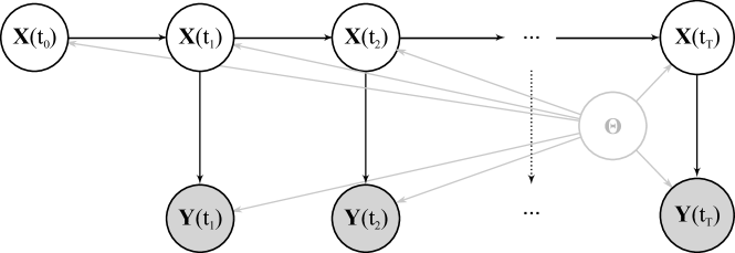
Figure 1: The state-space model, with parameters $\boldsymbol{\Theta}$, latent Markov state process $\mathbf{X}(t_{0:T})$ and observation process $\mathbf{Y}(t_{1:T})$.

2.1 Examples

Two example SSMs are introduced here. The first is a linear three-element windkessel model of arterial blood pressure [Westerhof2009], the second a nonlinear eight-dimensional Lorenz ’96 model of chaotic atmospheric processes [Lorenz2006]. In each case the original deterministic model is introduced, then stochasticity added, and a prior distribution over parameters specified, to massage it into the SSM framework.

2.1.1 Windkessel model

A windkessel model can be used to relate blood pressure and blood flow in the human arterial system [Westerhof2009]. The simplest two-element windkessel [Frank1899] is physically inspired: it couples a pump (the heart) and a chamber (the arterial system), with fluid (blood) flowing from the pump to the chamber, and returning via a closed loop. Air in the chamber is compressed according to the volume of fluid (analogous to the compliance of arteries).

The two-element windkessel model is commonly represented as an RC circuit as in Figure 2 (left). Voltage models blood pressure and current blood flow. A resistor models narrowing vessel width in the periphery of the arterial system, and a capacitor the compliance of arteries.

Figure 2: Windkessel models represented as circuit diagrams, (left) two-element, and (right) three-element. $P_{a}(t)$ gives aortal pressure and $P_{p}(t)$ peripheral pressure. $F(t)$ gives blood flow.

The equations of the two-element windkessel are readily derived from circuit theory applied to Figure 2 (left) [Kind2010]:

$$\frac{1}{R}P_{p}(t)+C\frac{dP_{p}(t)}{dt}=F(t).$$

This is a linear differential equation. Assuming a discrete time step $\Delta t$ and constant flow $F$(t) over the interval $[t,t+\Delta t)$, it may be solved analytically to give:

$$P_{p}(t+\Delta t)=\exp\left(-\frac{\Delta t}{RC}\right)P_{p}(t)+R\left(1-\exp\left(-\frac{\Delta t}{RC}\right)\right)F(t).$$ (3)

The two-element windkessel captures blood pressure changes during diastole (heart dilatation) well, but not during systole (heart contraction) [Westerhof2009]. An improvement is the three-element windkessel in Figure 2 (right), which introduces additional impedence from the aortic valve. Again using circuit theory, aortal pressure, $P_{a}$, may be related to peripheral pressure, $P_{p}$, by [Kind2010]:

$$P_{a}(t)=P_{p}(t)+F(t)Z.$$ (4)

The three-element windkessel is adopted henceforth. Blood flow, $F(t)$, would usually be measured, but for demonstrative purposes it is simply prescribed the following functional form:

$$F(t)=\begin{cases}F_{\text{max}}\sin^{2}\left(\frac{\pi t}{T_{s}+T_{d}}\right)&\text{if }\mathrm{mod}(t,T_{s}+T_{d})\in[0,T_{s}]\\ 0&\text{if }\mathrm{mod}(t,T_{s}+T_{d})\in(T_{s},T_{s}+T_{d}),\end{cases}$$ (5)

where $F_{\text{max}}=500\,\text{ml s}^{-1}$ gives maximum flow, $T_{s}=0.3\,\text{s}$ is time spent in systole, $T_{d}=0.5\,\text{s}$ is time spent in diastole, with $\mathrm{mod}(x,y)$ giving the non-integer part of $x/y$. This models quickly increasing then decreasing blood flow during systole, and no flow during diastole. The function is discretised to time steps of $\Delta t$ and held constant in between.

An SSM can be constructed around the above equations. Input $F(t)$ is prescribed as above, and a Gaussian noise term $\xi(t)$ of zero mean and variance $\sigma^{2}$ is introduced to extend the state process from deterministic to stochastic behaviour (details below). The SSM has parameters $\boldsymbol{\Theta\equiv}\left(R,C,Z,\sigma^{2}\right)^{T}$, state $\mathbf{X}(t)\equiv P_{p}(t)$ and observation $\mathbf{Y}(t)\equiv P_{a}(t)$. The time step is fixed to $\Delta t=10^{-2}$s.

The complete model is specified in the LibBi modelling language in Figure LABEL:fig:windkessel-bi. The specification begins with a model statement to name the model. It proceeds with the time step size declared on line 5 as a constant value. Following this, the four parameters of the model, R ($R$), C ($C$), Z ($Z$) and sigma2 ($\sigma^{2}$) are declared on lines 7-10, the input F ($F$(t)) on line 11, the noise term xi ($\xi(t)$) on line 12, the state variable Pp ($P_{p}(t)$) on line 13, and the observation Pa ($P_{a}(t)$) on line 14.

Windkessel.bi

 

1 /**
    2  * Three-element Windkessel model.
    3  */
    4 model Windkessel {
    5   const h = 0.01  // time step (s)
    6 
    7   param R         // peripheral resistance, mm Hg (ml s**-1)**-1
    8   param C         // arterial compliance, ml (mm Hg)**-1
    9   param Z         // characteristic impedence, mm Hg s ml**-1
   10   param sigma2    // process noise variance, (mm Hg)**2
   11   input F         // aortic flow, ml s**-1
   12   noise xi        // noise, ml s**-1
   13   state Pp        // peripheral pressure, mm Hg
   14   obs Pa          // observed aortic pressure, mm Hg
   15 
   16   sub parameter {
   17     R ~ gamma(2.0, 0.9)
   18     C ~ gamma(2.0, 1.5)
   19     Z ~ gamma(2.0, 0.03)
   20     sigma2 ~ inverse_gamma(2.0, 25.0)
   21   }
   22 
   23   sub initial {
   24     Pp ~ gaussian(90.0, 15.0)
   25   }
   26 
   27   sub transition(delta = h) {
   28     xi ~ gaussian(0.0, h*sqrt(sigma2))
   29     Pp <- exp(-h/(R*C))*Pp + R*(1.0 - exp(-h/(R*C)))*(F + xi)
   30   }
   31 
   32   sub observation {
   33     Pa ~ gaussian(Pp + Z*F, 2.0)
   34   }
   35 
   36   sub proposal_parameter {
   37     R ~ truncated_gaussian(R, 0.03, lower = 0.0)
   38     C ~ truncated_gaussian(C, 0.1, lower = 0.0)
   39     Z ~ truncated_gaussian(Z, 0.002, lower = 0.0)
   40     sigma2 ~ inverse_gamma(2.0, 3.0*sigma2)
   41   }
   42 }