A slope conjecture for links
Abstract
The slope conjecture [7] gives a precise relation between the degree of the colored Jones polynomial of a knot and the boundary slopes of essential surfaces in the knot complement. In this note we propose a generalization of the slope conjecture to links. We prove the conjecture for all alternating or more generally adequate links. We also verify the conjecture for torus links.
1 Introduction
As predicted by Witten’s path integral formulation [17], the (colored) Jones polynomial provides many relations between classical and quantum topology. For example the AJ conjecture relates the -difference equation for the colored Jones polynomials to the character variety of the knot group [5, 2]. A closely related but perhaps more tractable problem is the slope conjecture [7]. The slope conjecture gives an interpretation of the growth of the maximal degree of the the colored Jones polynomials in terms of essential surfaces in the knot complement. The purpose of this note is to suggest a generalization of the slope conjecture to links.
Let be a link in with components. For a link in , let denote a tubular neighborhood of and let denote the exterior of . The boundary is a union of tori, one for each component of . Let be the canonical meridian and longitude for the -th torus component .
Definition 1.
Suppose there exists a properly embedded essential surface , such that every circle of is homologous to . Then we call the sequence a boundary slope of .
Next consider the colored Jones function , see Section 2 for the definition. It sends a sequence of colors to the unnormalized colored Jones polynomial . Here each component is assumed to be -framed. For example if is the Hopf link, then and
The quadratic behaviour of the maximal degree in of is described in the following definition.
Definition 2.
A slope matrix for a function is an symmetric matrix if there exist infinite subsets and a constant such that for we have .
We are interested in slope matrices for functions . In the Hopf link example the funciton has a single slope matrix given by . Indeed, the maximal degree is roughly for all so we can take and .
We are now ready to formulate the slope conjecture for links.
Conjecture 1.
(Slope conjecture for links)
If is a slope matrix for then there exists an essential
surface in the complement of whose boundary slope is given by the column sums
of the slope matrix. So -th element of the boundary slope equals .
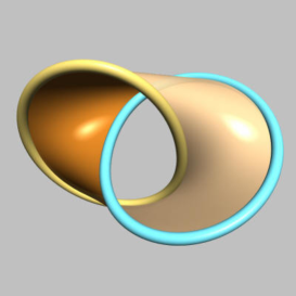
For example the above slope matrix for the maximal degree of the Hopf link should yield a surface with slope , the column sums of the slope matrix. In Figure 1 we have drawn such a surface.
In the case of a knot a slope matrix for coincides with an accummulation point of the set . Therefore our slope conjecture for links generalizes the original slope conjecture for knots as stated in [7]. here is a similar statement for the minimal degree of the knot but this follows from the present conjecture by replacing the knot by its mirror image.
To provide some evidence for our conjecture we prove it for the large class of -adequate links by generalizing the proof of [3] to links. Minus-adequate links are a vast generalization of alternating links, see Section 3 for a precise definition.
Theorem 1.
The slope conjecture is true for all minus-adequate links.
Given the simple closed form for torus links it is not hard to check the conjecture holds in this case as well.
Theorem 2.
The slope conjecture holds for all torus links.
As additional evidence for the conjecture we note that if we take two knots for which the slope conjecture is known then the slope conjecture also holds for their distant union. This is because the colored Jones polynomial is multiplicative and the slopes additive. Connected sum can also be checked along the lines of [13].
From these examples and theorems it may appear that the degree is rather well behaved and easy to compute from the state sums
and the surfaces are simply some Seifert-type state surfaces. In the general case this is quite far from the truth.
Massive cancellations will usually render the ordinary state sums useless. Also the surfaces are in general quite complicated as the slopes are often
rational numbers with high denominator [9]. As such the slope conjecture presents a major challenge to both classical and quantum topology.
Acknowledgement A preliminary version of this work was presented at the Moab topology conference 2012. I would like to thank the organizers Nathan Geer and Jessica Purcell for their hospitality and for providing an inspiring atmosphere. I would also like to thank Oliver Dasbach, Dave Futer, Stavros Garoufalidis, Effie Kalfagianni and Jessica Purcell for stimulating conversations. This work was supported by the Netherlands Organisation for Scientific Research.
2 Colored Jones polynomial for links
Since multiple conventions are in use in the literature we briefly give a definition of the colored Jones polynomial of a link. The present definition is perhaps not the most natural but has the advantage of being relatively concrete and easy to state. Assuming the reader is familiar with simple skein theory [12] it is easiest to construct the colored Jones polynomial from the colored Kauffman bracket as follows.
Recall that the skein space of the annulus can be regarded as the polynomial ring in the variable corresponding to its core. Given a framed knot diagram we can insert an element of the skein of the annulus and take the Kauffman bracket in the plane. The resulting Laurent polynomial in will be written . More generally for a -component link diagram and polynomial , on for each component we will write .
Because of representation theory a special role is played by the Chebyshev polynomials defined by and and .
Definition 3.
-
Let be an -component link in with diagram where the writhe of the -th component is .
-
1.
The -colored Kauffman bracket of is defined to be
-
2.
Set . The -colored Jones polynomial of an -component link is defined to be
Note the shift from to . The version of the colored Jones polynomial we defined is unnormalized and framing independent because of the writhe term. The value of the -colored unknot is . It is perhaps more standard to replace by but the variable neatly absorbs the factor of otherwise present in the slope conjecture.
3 Proof of the slope conjecture for minus-adequate links
Recall that in computing the Kauffman bracket each crossing gets resolved in two different ways: the plus-resolution and the minus-resolution (also known as the - and -resolutions). The result is a linear combination, the state sum, where each resolution contributes . A diagram is called minus-adequate (also -adequate) if after taking the minus-resolution everywhere, the two arcs replacing each crossing always belong to different circles. In other words, the all minus-resolution results in the maximal number of state circles. As such it must contribute the lowest power of , namely where is the number of crossings and is the number of circles in the state. See Lemma 5.4 [12].
Finally recall that the minus-state surface is the surface obtained from the diagram by the following steps. First do the all minus-resolution and turn each of the resulting circles into disks. Next at each former crossing, attach a half twisted band connecting a pair of disks. This surface is essential according to Ozawa [14], see also [4] Theorem 3.19.
We are now ready to prove the slope conjecture for minus-adequate links. Our proof generalizes that for knots found in [3].
Let be a -adequate link diagram whose all minus-resolution gives rise to state circles. We assume the link has components and we denote the diagram of the -th component by . Also and are the number of positive and negative crossings between and . The total number of such crossings is and the writhe is .
If we denote by the -parallel of the diagram (component gets replaced by parallel copies) then
This is because we can expand the Chebyshev polynomials into a linear combination of minus-adequate diagrams. Since the all minus-resolution yields the lowest degree term for each diagram, the overall lowest degree is that of the leading term of the Chebyshev polynomial. Moreover we know exactly what this minimal degree of the Kauffman bracket is: minus the number of crossings minus twice the number of state circles:
We can estimate where is the number of state circles in the minus-resolution of itself.
Summing up we found the following estimate for the maximal degree in of :
In other words the matrix defined below is a slope matrix in the sense of Definition 2.
For this we take the infinite subsets from the definition to be and choose some constant .
In order to prove Theorem 1 we now need to find an essential surface whose slope at the -th component equals . For this we can use the all minus-state surface introduced above. The slope of this surface is found by calculating the linking number between the -th component and a curve following it along the surface. For every negative crossing between and itself we find a contribution of . For positive such crossings we get a contribution of . For any type of crossing between and another component we obtain a contribution . In total one thus gets a slope of as required.
4 The case for torus links
We consider the -torus link with and to be the closure of the braid in . In case the standard braid diagram is minus-adequate. If follows from the formula of the Jones polynomial below that the case is not minus-adequate and hence provides additional evidence to our version of the slope conjecture for links.
The link has components. If we define and then the colored Jones polynomial colored by is given by the formula [15]
where the summation variable takes steps of two and we used the notation and and finally is the coefficient of in .
For we see that the maximal degree is given by the term . This term has maxdegree . Hence the unique slope matrix is given by . This is in agreement with Theorem 1 applied to the standard braid diagram. Hence the state-surface provides the surface with the correct slopes .
The case is more interesting. The formula for the maximal degree is not a quadratic polynomial in but is piecewise quadratic depending on the parity of . This already shows that such links cannot be minus-adequate since then the degree would be a quadratic polynomial in .
More specifically if is even then maximal degree is given by the term and equals . Care has to be taken with the case since there the term contributes with the same degree but luckily with a different coefficient: For and we have .
Next we look at the case odd. The term contributes the maximal degree which now equals , except in the cases . By the symmetry between and we may assume that in which case the term vanishes. The term then contributes
In either case the correct slope matrix is . To complete the slope conjecture we need to find an incompressible surface bounding the link whose boundary slopes are all . Consider the canonical annuli defined by taking the complement of the torus link viewed as sitting on the torus surface. This surface is certainly essential and each component is seen to have slope as required. This proves Theorem 2.
With a bit more work one may be able to prove the slope conjecture for all zero-volume links as these are very similar to torus links. Their colored Jones polynomials can be readily computed by repeatedly cabling and taking connected sums, see [15].
5 Further directions
Computing boundary slopes of surfaces in link complements is an interesting problem in classical topology. Outside the knot case not much is known except for some work on the two-bridge link case [10]. Through the slope conjecture one can use the colored Jones polynomial to explore such slopes further. At least in some cases [9] the Jones polynomial suggests the existence of some very non-trivial slopes, thus providing new challenges to classical topology.
One wonders if there a way to extract these slopes from the tropical geometry of the A-ideal that replaces the A-polynomial in the link case. This is natural since one expects an AJ-type conjecture for links.
On the colored Jones side an important question is whether the degree is still a (multivariate) quadratic quasipolynomial as in the knot case [6]. At least for minus-adequate links and the torus links we considered this is true. Such a question brings us back to a possible link version of the AJ conjecture. An important first step towards such a conjecture has been set for two-bridge links in [11].
It would also be interesting to go beyond the slope conjecture as in [8] and consider stabilization properties for links. At least for alternating links their (multivariate) heads and tails and beyond can readily be computed.
Finally the question of the behaviour of the degree can be posed for any quantum invariant, not just the colored Jones polynomial. It would be interesting to see what happens for other knot polynomials and their categorifications. A first approach to this question in the colored HOMFLY case has been made in [16].
References
- [1] Arjeh Cohen and Jarke van Wijk. Visualization of Seifert surfaces. IEEE Trans. on Visualization and Computer Graphics, 12:485–496, 2006.
- [2] Charles Frohman, Razvan Gelca, and Walter Lofaro. The A-polynomial from the noncommutative viewpoint. Trans. Amer. Math. Soc., 354:735–747, 2002.
- [3] Dave Futer, Efstratia Kalfagianni, and Jessica Purcell. Slopes and colored Jones polynomials of adequate knots. Proc. Amer. Math. Soc., 139:1889–1896, 2011.
- [4] Dave Futer, Efstratia Kalfagianni, and Jessica Purcell. Guts of surfaces and the colored Jones polynomial, volume 2069 of Lecture Notes in Mathematics. Springer, 2013.
- [5] Stavros Garoufalidis. On the characteristic and deformation varieties of a knot. Geom. Topol. Monogr., 7:291–309, 2004.
- [6] Stavros Garoufalidis. The degree of a q-holonomic sequence is a quadratic quasi-polynomial. Electronic Journal of Combinatorics, 18:4–27, 2011.
- [7] Stavros Garoufalidis. The Jones slopes of a knot. Quantum Topology, 2:43–69, 2011.
- [8] Stavros Garoufalidis and Thang Le. Nahm sums, stability and the colored Jones polynomial. arXiv 1112.3905, 2011.
- [9] Stavros Garoufalidis and Roland van der Veen. Quadratic integer programming and the slope conjecture. arXiv 1405.5088, 2014.
- [10] Jim Hoste and Patrick Shanahan. Computing boundary slopes of 2-bridge links. Mathematics of Computation, 76:1521–1545, 2007.
- [11] Thang Le and Ahn Tran. The Kauffman bracket skein module of two-bridge links. arXiv:1111.0332, 2011.
- [12] W. Raymond Lickorish. An Introduction to Knot Theory. Springer, 1997.
- [13] Kimihiko Motegi and Toshie Takata. Cabling, connected sum operations and the slope conjecture. arXiv 1501.01105, 2015.
- [14] Makoto Ozawa. Essential state surfaces for adequate knots and links. J. Australian Math. Soc., 91:391–404, 2011.
- [15] Roland van der Veen. A cabling formula for the colored Jones polynomial. arXiv:0807.2679, 2008.
- [16] Roland van der Veen. The degree of the colored HOMFLY polynomial. arXiv:1501.00123, 2015.
- [17] Edward Witten. Quantum field theory and the Jones polynomial. Comm. Math. Phys., 121:351–399, 1989.