Interacting viscous dark fluids

Abstract

We revise the conditions for the physical viability of a cosmological model in which dark matter has bulk viscosity and also interacts with dark energy. We have also included radiation and baryonic matter components; all matter components are represented by perfect fluids, except the dark matter, that is treated as an imperfect fluid. We impose upon the model the condition of a complete cosmological dynamics that results in an either null or negative bulk viscosity, but the latter also disagrees with the Local Second Law of Thermodynamics. The model is also compared with cosmological observations at different redshifts: type Ia supernova, the shift parameter of CMB, the acoustic peak of BAO, and the Hubble parameter $H(z)$. In general, observations consistently point out to a negative value of the bulk viscous coefficient, and in overall the fitting procedure shows no preference for the model over the standard $\Lambda$CDM model.

I Introduction

Cosmological models with interacting dark components have gained interest because it is expected that the most abundant components in the present Universe, dark energy (DE) and dark matter (DM), interact with each other, and some authors claim that some of these interaction terms are promising mechanisms to solve the $\Lambda$CDM problems (see for instanceChimento et al. (2000); *Copeland:2006wr; *Tsujikawa:2010sc; Kremer and Sobreiro (2012) and references therein).

On the other hand, it has been known since before the discovery of the present accelerated expansion of the Universe that a bulk viscous fluid may induce an accelerating cosmology Heller and Klimek (1975); *Barrow1986; *Visco-Padmanabhan1987; *Visco-Gron1990; *Visco-Maartens1995; *Visco-Zimdahl1996. Hence, it has been proposed that the bulk viscous pressure can be one of the possible mechanism to accelerate the Universe today (see for instance Cataldo et al. (2005); Colistete et al. (2007); *AvelinoUlises1P:2008; Avelino and Nucamendi (2010); *Visco-RicaldiVeltenZimdahl2010; *Visco-AMontielNBreton2011). However, this idea still needs of some physically motivated model to explain the origin of the bulk viscosity. In this sense some proposals have been already put forward inZimdahl (2000); *Mathews:2008hk.

In the present work, we have the interest to explore and test an interacting dark sector model which also takes into account a bulk viscosity in the DM component. Our study is two fold: first, we explore the general conditions for the model to have a complete cosmological dynamics, and second, we use cosmological observations to fit the free parameters of the model.

We have called complete cosmological dynamics to the fact that all physically viable model must allow the existence of radiation and matter domination eras at early enough times, so that the known processes of the early Universe are not significantly changed with respect to those of the standard Big Bang model. This seems to be an usually overlooked condition in most studies of alternative cosmological models, for which the primary concern is the present accelerated expansion of the Universe, and then it is commonly thought that a low-redshift analysis is quite enough for the task.

The full dynamics of the model is found through a dynamical system analysis, a common tool in the analysis of cosmological modelsCopeland et al. (1998); *Wainwright:1997; *Coley:1999uh; *UrenaLopez:2005zd; *Matos:2009hf; Caldera-Cabral et al. (2009); *Caldera-Cabral2010, and then the DM-DE interaction term is chosen such as to allow the writing of the equations of motion as an autonomous set of differential equations. We are then able to write general conditions for the existence of radiation and matter eras at early times that are useful for a wide variety of interacting models.

The bulk viscous coefficient in our model is directly proportional to the Hubble parameter, and we impose upon it a constraint that comes from the Local Second Law of Thermodynamics (LSLT). In general, as it also happens for our model, this latter condition selects only positive definite values of the bulk viscous coefficientIsrael and Stewart (1979); *Visco-Israel1987; *Visco-Maartens1996b; Misner and Wheeler (1973); *WeinbergBook.

The model is also compared with different cosmological observations: type Ia supernovae, the shift parameter of CMB, the acoustic peak of BAO, and the Hubble parameter $H(z)$, in order to constraint its free parameters. As we shall show, the fitted values acquire different values depending on whether we use low-redshift or intermediate-redshift observations. In a similar way as in the condition for a complete cosmological dynamics, wrong conclusions may be obtained if the analysis is only made with observations in the lowest range of redshifts (late times).

The paper is organized as follows. In Sec. II we present the full characteristics of the model, the main equations of motion, and the dynamical system analysis. The bulk viscosity of the model is represented by a single free parameter, whereas the DM-DE interaction term is considered a free function of the DM and DE density parameters, as long as the dynamical system of equations remains autonomous. The cosmological eras of the model are given in terms of the critical points of the dynamical system, whose existence conditions depend upon the values of the free parameters of the model. A detailed discussion about the existence or not of appropriate cosmological eras is provided in terms of the aforementioned constraint of a complete cosmological dynamics.

In Sec. III, we focus our attention in a particular form for the DM-DE interacting term that is directly proportional to the DE energy density. Full details are given about the existence and stability of the critical points, which are in turn transformed into conditions upon the free parameters of the model. Also, we show some particular examples of the dynamics of the model for selected values of the free parameters.

We explain in Sec. IV the cosmological probes that are used to constrain the model, and give separate examples of the fitting procedure for different sub-cases of the model. For completeness, we include here low and intermediate redshift constraints, so that we can track the changes in the values of the parameters for those cases. Finally, the main results are summarized and discussed in Sec. V.

II Interacting bulk viscous dark fluids

We study a cosmological model in a spatially flat Friedmann-Robertson-Walker (FRW) metric, in which the matter components are radiation, baryons, DM, and DE. Except to the DM, all energy-matter components will be characterized by perfect fluids: radiation and baryons are assumed to have the usual properties, whereas DM is treated as an imperfect fluid having bulk viscosity, with a null hydrodynamical pressure, and interacting with DE. This phenomenological model is a natural extension of that proposed by Kremer and SobreiroKremer and Sobreiro (2012).

The Friedmann constraint and the conservation equations for the matter fluids can be written as

$$H^{2} = \frac{8\pi G}{3}\left(\rho_{\rm r}+\rho_{\rm b}+\rho_{\rm dm}+\rho_{\rm de}\right)\,,$$ (1a)

$$\dot{\rho}_{\rm r} = -4H\rho_{\rm r}\,,$$ (1b)

$$\dot{\rho}_{\rm b} = -3H\rho_{\rm b}\,,$$ (1c)

$$\dot{\rho}_{\rm dm} = -3H\rho_{\rm dm}+Q-3H(-3H\zeta)\,,$$ (1d)

$$\dot{\rho}_{\rm de} = -3H\gamma_{\rm de}\rho_{\rm de}-Q$$ (1e)

where $G$ is the Newton gravitational constant, $H$ the Hubble parameter, $(\rho_{\rm r},\rho_{\rm b},\rho_{\rm dm},\rho_{\rm de})$ are the energy densities of the radiation, baryon, DM, and DE fluid components, respectively, and $\gamma_{\rm de}$ is the barotropic index of the equation of state (EOS) of DE, which is defined from the relationship $p_{\rm de}=(\gamma_{\rm de}-1)\rho_{\rm de}$, where $p_{\rm de}$ is the pressure of DE. The term $-3H\zeta$ in Eq. (1d) corresponds to the bulk viscous pressure of the dark matter fluid, with $\zeta$ the bulk viscous coefficient, whereas $Q$ is the DM-DE interaction term.

We consider the bulk viscous coefficient $\zeta$ as proportional to the total matter density, $\rho_{\rm t}=\rho_{\rm r}+\rho_{\rm b}+\rho_{\rm dm}+\rho_{\rm de}$, in the form

$$\zeta=\frac{\zeta_{0}}{\sqrt{24\pi G}}\rho^{1/2}_{\rm t}=\left(\frac{1}{8\pi G}\right)H\zeta_{0}\,,$$ (2)

where $\zeta_{0}$ is a dimensionless constant to be estimated from the comparison with cosmological observations. From Eq. (1a), we can see that this parametrization corresponds to a bulk viscosity proportional to the expansion rate of the Universe, i.e., to the Hubble parameter. Finally, the Raychadury equation of the model is

$$\dot{H}=-4\pi G\left(\frac{4}{3}\rho_{\rm r}+\rho_{\rm b}+\rho_{\rm dm}+\gamma_{\rm de}\rho_{\rm de}-3H\zeta\right)\,.$$ (3)

In our analysis, we will take into account an important restriction over the bulk viscous coefficient that comes from the Local Second Law of Thermodynamics (LSLT). The local entropy production for a fluid on a FRW space–time is expressed asWeinberg (1972); Misner and Wheeler (1973)

$$T\,\nabla_{\nu}s^{\nu}=\zeta(\nabla_{\nu}u^{\nu})^{2}=9H^{2}\zeta\,,$$ (4)

where $T$ is the temperature of the fluid, and $\nabla_{\nu}s^{\nu}$ is the rate of entropy production in a unit volume. Then, the second law of the thermodynamics can be stated as $T\nabla_{\nu}s^{\nu}\geq 0$; since the Hubble parameter $H$ is positive for an expanding Universe, Eq. (4) implies that $\zeta\geq 0$. For the present model, this inequality in turn becomes (see Eq. (2))

$$\zeta_{0}\geq 0\,.$$ (5)

II.1 The dynamical system perspective

In order to study all possible cosmological scenarios of the model, we proceed to a dynamical system analysis of Eqs. (1) and (3). Let us first define the set of dimensionless variables:

$$x = \frac{8\pi G}{3H^{2}}\rho_{\rm de}\,,\quad y=\frac{8\pi G}{3H^{2}}\rho_{\rm dm}\,,$$ (6a)

$$u = \frac{8\pi G}{3H^{2}}\rho_{\rm b}\,,\quad z=\frac{8\pi G}{3H^{3}}Q\,.$$ (6b)

Then, the equations of motion can be written in the following, equivalent, form:

$$\frac{dx}{dN} = -z+x(4-u-y-3\gamma_{\rm de}-3\zeta_{0})-x^{2}(4-3\gamma_{\rm de})\,,$$ (7a)

$$\frac{dy}{dN} = y(1-u-y-x(4-3\gamma_{\rm de})-3\zeta_{0})+z+3\zeta_{0}\,,$$ (7b)

$$\frac{du}{dN} = u(1-u-y-x(4-3\gamma_{\rm de})-3\zeta_{0})\,,$$ (7c)

where the derivatives are with respect to the $e$-folding number $N\equiv\ln a$. In term of the new variables, the Friedmann constraint (1a) can be written as:

$$\Omega_{\rm r}=\frac{8\pi G}{3H^{2}}\rho_{\rm r}=1-x-y-u\,,$$ (8)

and then we can choose $(x,y,u)$ as the only independent dynamical variables.

Taking into account that $0\leq\Omega_{\rm r}\leq 1$, and imposing the conditions that both the DM and DE components are both positive definite and bounded at all times, we can define the phase space of Eqs. (7) as:

$$\Psi = \{(x,y,u):0\leq 1-x-y-u\leq 1,0\leq x\leq 1\,,$$ (9)

$$0\leq y\leq 1,0\leq u<1\}\,.$$

Other cosmological parameters of interest are the total effective EOS, $w_{eff}$, and the deceleration parameter, $q=-(1+\dot{H}/H^{2})$, which can be written, respectively, as

$$w_{eff} = \frac{1}{3}(1-u-y-x(4-3\gamma_{\rm de})-3\zeta_{0})\,,$$ (10a)

$$q = \frac{1}{2}\{2-u-y-x(4-3\gamma_{\rm de})-3\zeta_{0}\}\,.$$ (10b)

In order to obtain an autonomous system of ordinary differential equations from Eqs. (7), we will focus our attention hereafter only in general interaction functions of the form $Q=3Hf(\rho_{dm},\rho_{de})$ that can lead to closed functions $z=z(x,y)$. As we shall see in the next section, this election will allow us to impose general conditions over the variable $z$ (and on the $Q$-term as well) in order to achieve a well behaved dynamics (seeCaldera-Cabral et al. (2009) for a similar exercise). Some examples of the interaction $Q$ that lead to the desired form of $z$ are listed in Table 1.

Table 1: Some proposed forms of $Q(\rho_{de},\rho_{dm})$ for which the dynamical system (7) becomes an autonomous system of differential equations.

Model	$Q(\rho_{de},\rho_{dm})$	$z(x,y)$	References
i	$3H(\alpha_{1}\rho_{de}+\alpha_{2}\rho_{dm})$	$3(\alpha_{1}x+\alpha_{2}y)$	Quartin et al. (2008); Caldera-Cabral et al. (2009); *Caldera-Cabral2010
ii	$3H\lambda\frac{\rho_{de}\rho_{dm}}{\rho_{de}+\rho_{dm}}$	$3\lambda\frac{xy}{x+y}$	Zimdahl and Pavon (2003)
iii	$3H\lambda\rho_{dm}$	$3\lambda y$	Zimdahl and Pavon (2001); Guo et al. (2007)

II.2 General conditions for a complete cosmological dynamics

If the system of equations (7) is autonomous, one then expects that important stages in the evolution of the model be represented by critical points in phase space. We will work on this hypothesis here to make a description of the existence, or not, of the different domination eras that have to be present in any model of physical interest.

We then demand that our model must follow a complete cosmological dynamics, namely: it should start in a radiation dominated era (RDE), later enter into a matter dominated era (MDE), and finally enter into the present stage of accelerated expansion; every one of these statements can be translated in definite mathematical equations, that we are going to discuss in detail in the sections below.

Before that, we need to calculate the critical points $(x_{*},y_{*},u_{*})$ of the dynamical system (7), which are to be found from the conditions:

$$0 = -z_{*}+x_{*}(4-u_{*}-y_{*}-3\gamma_{de}-3\zeta_{0})-x_{*}^{2}(4-3\gamma_{de})\,,$$ (11a)

$$0 = y_{*}(1-u_{*}-y_{*}-x_{*}(4-3\gamma_{de})-3\zeta_{0})+z_{*}+3\zeta_{0}\,,$$ (11b)

$$0 = u_{*}(1-u_{*}-y_{*}-x_{*}(4-3\gamma_{de})-3\zeta_{0})\,,$$ (11c)

where $z_{*}\equiv z(x_{*},y_{*},u_{*})$ is the interaction variable evaluated at the critical points, see Eqs. (6).

II.2.1 Radiation domination

Let us start with the conditions for a purely RDE. According to the Friedmann constraint (8), a purely RDE with $\Omega_{r}=1$ corresponds to $(x_{*},y_{*},u_{*})=(0,0,0)$, and then Eqs. (11) further dictate that

$$z_{*}=0\,,\quad z_{*}=-3\zeta_{0}\,.$$ (12)

The first condition on the DM-DE interaction term holds for many of the interacting functions $z=z(x,y)$ in the specialized literature, like for those examples listed in Table 1; but the second condition strongly implies that it is not possible to reconcile a purely RDE with a non-zero bulk viscosity, $\zeta_{0}\neq 0$.

However, there are other less extreme possibilities for radiation domination in which a bulk viscosity exists, as long as we allow the coexistence of radiation and other matter components early in the evolution of the Universe.

As the bulk viscosity term only appears actively for the equation of motion of DM, see Eqs. (7b) and (11b), we see that the early presence of DM could allow the existence of bulk viscosity in a RDE. The critical point we are looking for is of the form $(x_{*},y_{*},u_{*})=(0,y_{*},0)$, under the assumption $y_{*}\ll 1$, and then we obtain the following conditions,

$$y_{*}=-3\zeta_{0}\,,\quad z_{*}=0\,.$$ (13)

Thus, a RDE is possible as long as the DM-DE interacting term is null, and the bulk viscosity is negative, $\zeta_{0}<0$ (in order to preserve the condition $y\geq 0$). However, this is at variance with the condition from the LSLT in Eq. (5).

The null condition for the interaction term can be obtained if $z$ is a function with mixed $x-y$ terms like that of Model (ii) in Table 1, or with a dependence only on $x$, an instance of which is Model (i) with $\alpha_{2}=0$.

Another possible critical point for a RDE would be $(x_{*},y_{*},u_{*})=(x_{*},0,0)$, which by means of Eqs. (11), leads to the conditions

$$x_{*}=\frac{-3\zeta_{0}}{4-3\gamma_{de}}\,,\quad z_{*}=-3\zeta_{0}\,.$$ (14)

As the DE EOS satisfies $\gamma_{de}<1$, then a RDE is achieved if $x_{*}\ll 1$ and $\zeta_{0}<0$, but the latter condition is again at variance with the LSLT in Eq. (5).

II.2.2 Matter domination

The existence of a MDE requires a scaling relation between the baryonic and CDM densities in the form $(x_{*},y_{*},u_{*})=(0,\beta,1-\beta)$, where $\beta\;\in\;[0,1]$, so that $y_{*}+u_{*}=1$, as dictated by the Friedmann constraint (8). This time, Eqs. (11) dictate that

$$0=-z_{*}\,,\quad 0=-3(1-\beta)\zeta_{0}\,,$$ (15)

are the simultaneous independent conditions to fulfill a MDE.

The first condition requires again the interaction term $z$ to be a function with mixed $x-y$ terms like that of Model (ii) in Table 1, or with a dependence only on $x$, like Model (i) with $\alpha_{2}=0$. For this latter case, and also Model (iii), a nonzero value of $\alpha_{2}$ needs a baryon dominated critical point, $(x_{*},y_{*},u_{*})=(0,0,1)$, which we consider as non-realistic.

The second condition allows two possibilities:

• $\zeta_{0}=0$. As in the condition for a successful RDE, the model needs a null bulk viscosity to reach a correct MDE.

• $\beta=1$ ($\forall\;\zeta_{0}\;\in\;[0,\infty)$) represents a critical point of pure CDM domination, which is at variance with the well established fact that baryons have a non negligible contribution to the matter contents.

Another scenario to describe the MDE is an scaling relation among baryonic matter, CDM and DE. This requirement implies a fine tunning over the very small amount of DE allowed for this period, without preventing or slowing structure formation. This translates into $(x_{*},y_{*},u_{*})=(1-y_{*}-u_{*},y_{*},u_{*})$, so that $x_{*}+y_{*}+u_{*}=1$, as indicated by the Friedmann constraint (8). With the above values, Eqs. (11) lead to two independent possibilities:

• $z_{*}=3(1-y_{*})((1-\gamma_{de})y_{*}-\zeta_{0})$, and $u_{*}=0$. The null contribution of baryons, and the scaling relation between CDM and DE, suggest that it is impossible to recover a successful MDE, even though this critical point could correspond to a possible late time scenario.

• $z_{*}=3(1-\gamma_{de})(1-y_{*}-u_{*})$, and $x_{*}=\zeta_{0}/(\gamma_{de}-1)$. We have either: $\zeta_{0}>0$ and $\gamma_{de}>1$, which agrees with the LSLT in Eq. (5), but corresponds to a non realistic DE EOS, $w_{de}>0$; or $\zeta_{0}<0$ and $\gamma_{de}<1$, which violates Eq. (5), but somehow allows a valid MDE if $x_{*}\ll 1$.

II.2.3 Accelerated expansion

In order to describe the present stage of accelerated expansion, and at the same time alleviate the coincidence problem, we need a scaling regime between the DM and DE components. This requirement leads to the critical point $(x_{*},y_{*},u_{*})=(x_{*},1-x_{*},0)$, and then Eqs. (11) lead to the single condition:

$$z_{*}=3x_{*}(1-x_{*}-\gamma_{de}+x_{*}\gamma_{de}-\zeta_{0})\,.$$ (16)

This last equation can be solved once the interaction term is given for a particular model, and we can foresee that there must be valid solutions of it for any values, positive or negative, of the bulk viscosity constant $\zeta_{0}$. Moreover, if we impose the condition for strict DE domination, $x_{*}=1$, then $z_{*}=-3\zeta_{0}$; this can be possible, for instance, for Model (i) in Table 1.

II.2.4 Final comments

The requirement of a complete cosmological dynamics discussed above, from the dynamical system point of view, rules out any model that obeys the equations of motion (1), because the presence of the bulk viscosity blockades the existence of standard RDE and MDE, if we are to believe in the LSLT as stated in Eq. (5). It must be noticed, though, that an accelerated expansion of the Universe at low redshifts is indeed compatible with bulk viscosity.

In Secs. III and IV below, we will perform a full dynamical system analysis of the field equations for the particular case $Q=3H\alpha\rho_{de}$, and then we will show the importance of taking into account the full evolution of the Universe to constraint cosmological models.

III The case for $Q=3H\alpha\rho_{de}$

Table 2: Location, existence conditions according to the physical phase space (9), and stability of the critical points of the autonomous system (7a)-(7c) under $Q=3H\alpha\rho_{de}$. The eigenvalues of the linear perturbation matrix associated to each of the following critical points are displayed in Table 4.

$P_{i}$	$x$	$y$	$u$	Existence	Stability
$1a$	$0$	$-3\zeta_{0}$	$0$	$-\frac{1}{3}\leq\zeta_{0}\leq 0$	Unstable if $\zeta_{0}>-\frac{1}{3}$, $\alpha<\frac{4}{3}-\gamma_{de}$
					Saddle if $\zeta_{0}>-\frac{1}{3}$, $\alpha>\frac{4}{3}-\gamma_{de}$ or
$1b$	$x$	$-x-3\zeta_{0}$	$0$	$\gamma_{de}=1$, $\alpha=\frac{1}{3}$ and ($\zeta_{0}=0$, $x=0$ or	Removed from phase space
				$-\frac{1}{3}\leq\zeta_{0}<0$, $0\leq x\leq-3\zeta_{0}$)	See discussion in Sec. III.1
$1c$	$x$	$x(-4+3\gamma_{de})-3\zeta_{0}$	$0$	$\alpha=\frac{4}{3}-\gamma_{de}$, together with	Saddle if $\zeta_{0}<-\frac{1}{3}$
				those in Table 3 below.
$2a$	$0$	$1$	$0$	Always	Unstable if $\zeta_{0}<-\frac{1}{3}$, $\alpha<1-\gamma_{de}-\zeta_{0}$
					Stable if $\zeta_{0}>0$, $\alpha>1-\gamma_{de}-\zeta_{0}$
					Saddle if $\zeta_{0}<-\frac{1}{3}$, $\alpha>1-\gamma_{de}-\zeta_{0}$ or
					$-\frac{1}{3}<\zeta_{0}<0$, $\alpha\neq 1-\gamma_{de}-\zeta_{0}$ or
					$\zeta_{0}\geq 0$, $\alpha<1-\gamma_{de}-\zeta_{0}$
$2b$	$0$	$y$	$1-y$	$\zeta_{0}=0$, $0<y\leq 1$	Saddle if $\alpha<1-\gamma_{de}$
$2c$	$\frac{\zeta_{0}}{\gamma_{de}-1}$	$y$	$1-y-\frac{\zeta_{0}}{\gamma_{de}-1}$	$\alpha=1-\gamma_{de}$ and	Saddle if $\zeta_{0}>0$
				( $\zeta_{0}>0$, $0\leq y<1$, $\gamma_{de}\geq 1-\frac{\zeta_{0}}{y-1}$ or,
				$\zeta_{0}<0$, $0\leq y<1$, $\gamma_{de}\leq 1-\frac{\zeta_{0}}{y-1}$ or
				$\zeta_{0}=0$, $0<y\leq 1$, $\gamma_{de}\neq 1$ )
$2d$	$x$	$y$	$1-x-y$	$\zeta_{0}=\alpha=0$, $\gamma_{de}=1$ and	Removed from phase space
				( $y=1$, $x=0$ or $y=0$, $0<x\leq 1$ or	See discussion in Sec. III.1
				$0<y<1$, $0\leq x\leq 1-y$ )
$3a$	$1-\frac{\alpha+\zeta_{0}}{1-\gamma_{de}}$	$\frac{\alpha+\zeta_{0}}{1-\gamma_{de}}$	$0$	$\gamma_{de}<1$, $-\zeta_{0}\leq\alpha\leq 1-\gamma_{de}-\zeta_{0}$ or	Unstable if $\zeta_{0}>-\frac{1}{3}$, $\alpha>\frac{4}{3}-\gamma_{de}$ or
				$\gamma_{de}>1$, $1-\gamma_{de}-\zeta_{0}\leq\alpha\leq-\zeta_{0}$	$\zeta_{0}\leq-\frac{1}{3}$, $\alpha>1-\gamma_{de}-\zeta_{0}$
					Stable if $\zeta_{0}>0$, $\alpha<1-\gamma_{de}-\zeta_{0}$ or
					$\zeta_{0}\leq 0$, $\alpha<1-\gamma_{de}$
					Saddle if $\zeta_{0}>0$, $1-\gamma_{de}<\alpha<\frac{4}{3}-\gamma_{de}$ or
					$\zeta_{0}>0$, $1-\gamma_{de}-\zeta_{0}<\alpha<1-\gamma_{de}$ or
					$-\frac{1}{3}<\zeta_{0}\leq 0$, $1-\gamma_{de}-\zeta_{0}<\alpha<\frac{4}{3}-\gamma_{de}$ or
					$-\frac{1}{3}<\zeta_{0}<0$, $1-\gamma_{de}<\alpha<1-\gamma_{de}-\zeta_{0}$ or
					$\zeta_{0}\leq-\frac{1}{3}$, $1-\gamma_{de}<\alpha<\frac{4}{3}-\gamma_{de}$ or
					$\zeta_{0}<-\frac{1}{3}$, $\frac{4}{3}-\gamma_{de}<\alpha<1-\gamma_{de}-\zeta_{0}$
$3b$	$1-y$	$y$	$0$	$\alpha=-\zeta_{0}$, $\gamma_{de}=1$	Removed from phase space
					See discussion in Sec. III.1

Table 3: Existence conditions for the critical point $P_{1c}$ according to the physical phase space (9).

$P_{i}$	$Existence$
$1c$	($\zeta_{0}<-\frac{1}{3}$ and ( $\gamma_{de}<\frac{4}{3}-\zeta_{0}$, $\frac{1+3\zeta_{0}}{-3+3\gamma_{de}}\leq x\leq\frac{3\zeta_{0}}{-4+3\gamma_{de}}$ or $\gamma_{de}=\frac{4}{3}-\zeta_{0}$, $x=\frac{3\zeta_{0}}{-4+3\gamma_{de}}$ )) or
	($\zeta_{0}=-\frac{1}{3}$ and ($\gamma_{de}<1$, $0\leq x\leq\frac{1}{4-3\gamma_{de}}$ or $\gamma_{de}>1$, $x=0$)) or
	($-\frac{1}{3}<\zeta_{0}<0$ and ($0\leq x\leq 1$, $\gamma_{de}=\frac{4}{3}+\zeta_{0}$ or $0\leq x\leq\frac{3\zeta_{0}}{-4+3\gamma_{de}}$, $1<\gamma_{de}<\frac{4}{3}+\zeta_{0}$ or $0\leq x\leq\frac{3\zeta_{0}}{-4+3\gamma_{de}}$, $\gamma_{de}<1$ or
	$0\leq x\leq\frac{1+3\zeta_{0}}{-3+3\gamma_{de}}$, $\gamma_{de}>\frac{4}{3}+\zeta_{0}$)) or
	($\zeta_{0}=0$ and ($x=0$, $\gamma_{de}<1$ or $x=0$, $1<\gamma_{de}<\frac{4}{3}$ or $0\leq x\leq 1$, $\gamma_{de}=\frac{4}{3}$ or $0\leq x\leq\frac{1}{-3+3\gamma_{de}}$ )) or
	($\zeta_{0}>0$ and ($x=1$, $\gamma_{de}=\frac{4}{3}$ or $\frac{3\zeta_{0}}{-4+3\gamma_{de}}\leq x\leq\frac{1+3\zeta_{0}}{-3+3\gamma_{de}}$, $\gamma_{de}>\frac{4}{3}+\zeta_{0}$))

Table 4: Eigenvalues and some basic physical parameters for the critical points listed in Table 2, see also Eqs. (6) and (10).

$P_{i}$	$\lambda_{1}$	$\lambda_{2}$	$\lambda_{3}$	$w_{eff}$	$\Omega_{r}$	$q$
$1a$	$1$	$4-3\gamma_{de}-3\alpha$	$1+3\zeta_{0}$	$\frac{1}{3}$	$1+3\zeta_{0}$	$1$
$1b$	$1$	$0$	$1+3\zeta_{0}$	$\frac{1}{3}$	$1+3\zeta_{0}$	$1$
$1c$	$1$	$0$	$1+3\zeta_{0}$	$\frac{1}{3}$	$1-3x(\gamma_{de}-1)+3\zeta_{0}$	$1$
$2a$	$-1-3\zeta_{0}$	$-3\zeta_{0}$	$-3(-1+\gamma_{de}+\alpha+\zeta_{0})$	$-\zeta_{0}$	$0$	$\frac{1}{2}(1-3\zeta_{0})$
$2b$	$-1$	$0$	$-3(-1+\gamma_{de}+\alpha)$	$0$	$0$	$\frac{1}{2}$
$2c$	$-1$	$0$	$3\zeta_{0}$	$0$	$0$	$\frac{1}{2}$
$2d$	$-1$	$0$	$0$	$0$	$0$	$\frac{1}{2}$
$3a$	$3(-1+\gamma_{de}+\alpha)$	$-4+3\gamma_{de}+3\alpha$	$3(-1+\gamma_{de}+\alpha+\zeta_{0})$	$-1+\gamma_{de}+\alpha$	$0$	$\frac{1}{2}(-2+3\gamma_{de}+3\alpha)$
$3b$	$0$	$-1-3\zeta_{0}$	$-3\zeta_{0}$	$-\zeta_{0}$	$0$	$\frac{1}{2}(1-3\zeta_{0})$

This model of interaction was studied byKremer and Sobreiro (2012) in the context of interacting DM-DE with the presence of bulk viscosity. The model can be recovered from Model (i) in Table 1 with $\alpha_{1}=-\sqrt{3}\zeta_{0}$ and $\alpha_{2}=0$. Nonetheless, our study below generalizes the model inKremer and Sobreiro (2012) by taking a general interaction constant $\alpha$, and two new components in the cosmic inventory: radiation and baryonic matter. We will comment on the model ofKremer and Sobreiro (2012) at the end of this section.

The selected $Q$-term leads to the following dimensionless interaction variable $z$:

$$z=3\alpha x\,.$$ (17)

The nine critical points of the autonomous system (7), together with the interaction term in Eq. (17), are summarized in Table 2, whereas details about their stability and relevance for cosmology are given in Table 4.

III.1 Critical points and stability

The first point $P_{1a}$ corresponds to the co-existence of radiation and DM, and exists if the bulk viscosity takes values in the range $-\frac{1}{3}\leq\zeta_{0}\leq 0$. It also represents a decelerating expansion solution with $q=1$ and $w_{eff}=1/3$. Critical point $P_{1}$ exhibits two different stability behaviors

• Unstable if $\zeta_{0}>-\frac{1}{3}$ and $\alpha<\frac{4}{3}-\gamma_{de}$.

• Saddle if $\zeta_{0}>-\frac{1}{3}$ and $\alpha>\frac{4}{3}-\gamma_{de}$.

In this point, the dimensionless energy parameter for radiation and DM take the following values $\Omega_{r}=1+3\zeta_{0}$ and $\Omega_{\rm dm}=-3\zeta_{0}$ respectively, as shown in Table 4. Therefore this point could represent a true RDE if $\Omega_{\rm dm}\ll 1$, as long as $\zeta_{0}$ takes a negative value very close to zero, or, in the most extreme case, if $\Omega_{\rm dm}=0$ then $\zeta_{0}=0$, meaning no bulk viscosity. In both cases, the existence interval and the needed values for the bulk viscosity, to archive a successful RDE, are outside the region of validity of the LSLT ($\zeta_{0}>0$).

The non hyperbolic critical point $P_{1b}$ exists if $\gamma_{de}=1$ and $\alpha=\frac{1}{3}$. The first one condition is at odds with our expectation of a genuine DE fluid ($\gamma_{de}<1$), and then we will not take into account this critical point in our analysis.

$P_{1c}$ correspond to a decelerated solution ($q=1$) in which there is radiation, DM, and DE. In effective terms, this point is able to mimic the behavior of a radiation fluid ($w_{eff}=\frac{1}{3}$) but, a truly RDE is only reached if $x\ll 1$ and $-1\ll\zeta_{0}<0$, being the latter condition in contradiction with the LSLT. If $x=\frac{-3\zeta_{0}}{4-3\gamma_{de}}$, then this critical point reproduces the analysis developed in the previous section, see Eq. (14). Despite its non-hyperbolic nature, $P_{1c}$ always has a saddle behavior if $\zeta_{0}<-\frac{1}{3}$, since it possesses nonempty stable and unstable manifolds, see Table 4.

Critical point $P_{2a}$ represents a pure DM domination solution ($\Omega_{DM}=1$) and always exists, this fact is motivated by a null contribution of baryonic matter. The stability of this fixed point is the following:

• Saddle if $\zeta_{0}<-\frac{1}{3}$, $\alpha>1-\gamma_{de}-\zeta_{0}$ or
  $-\frac{1}{3}<\zeta_{0}<0$, $\alpha\neq 1-\gamma_{de}-\zeta_{0}$ or
  $\zeta_{0}\geq 0$, $\alpha<1-\gamma_{de}-\zeta_{0}$

• Stable if $\zeta_{0}>0$, $\alpha>1-\gamma_{de}-\zeta_{0}$.

• Unstable if $\zeta_{0}<-\frac{1}{3}$, $\alpha<1-\gamma_{de}-\zeta_{0}$.

An interesting fact of $P_{2a}$ is the value of the effective EOS parameter ($w_{eff}=-\zeta_{0}$): because of the non negative value of the bulk viscosity constant required by the LSLT, $w_{eff}\leq 0$, which means that we cannot recover a standard DM dominated picture, unless $\zeta_{0}=0$. $P_{2a}$ is represented by a red point in Fig. 1.

The non-hyperbolic fixed point $P_{2b}$ represents a scaling relation between the baryonic and DM components. As we claimed before in Sec. II, this critical point behaves as a realistic MDE and exists only under a null bulk viscosity contribution ($\zeta_{0}=0$). If $\alpha<1-\gamma_{de}$ this critical point has a saddle behavior.

$P_{2c}$ is a scaling solution between three components: baryons, DM, and DE, and, unlike point $P_{2b}$, it exists for all values of $\zeta_{0}$ (see Table 2 for the rest of existence conditions). This critical point could represent a feasible MDE if $x=\frac{\zeta_{0}}{\gamma_{de}-1}\ll 1$, and then $0<\zeta_{0}\ll 1$. This implies a fine tunning over the bulk viscosity parameter due to the negligible amount of DE that should exist during a MDE, which would render it almost indistinguishable from $P_{2b}$ in the phase space. This critical point exists given that:

• $\alpha=1-\gamma_{de}$, $\zeta_{0}>0$, $0\leq y<1$, $\gamma_{de}\geq 1-\frac{\zeta_{0}}{y-1}$. This region satisfies the LSLT (5), $\zeta_{de}>0$, but corresponds to a non truly DE component, $w_{de}>0$.

• $\alpha=1-\gamma_{de}$, $\zeta_{0}<0$, $0\leq y<1$, $\gamma_{de}\leq 1-\frac{\zeta_{0}}{y-1}$. This region violates LSLT (5) but allow a valid MDE if the above condition, $0<\zeta_{0}\ll 1$, is satisfied.

• $\alpha=1-\gamma_{de}$, $0<y\leq 1$, $\gamma_{de}\neq 1$ and $\zeta_{0}=0$.

Despite of its non-hyperbolic nature, the critical point always exhibits a saddle behavior if $\zeta_{0}>0$ since it has nonempty stable and unstable manifolds.

Critical point $P_{2d}$ corresponds to a very particular selection of the model parameters: $\alpha=\zeta_{0}=0$ and $\gamma_{de}=1$. These values represent a model with a null interaction between DM and DE, together with a null bulk viscosity contribution. The point $P_{2d}$ will not appear in the phase space as long as we take $\alpha\neq 0$ and $\zeta_{0}\neq 0$.

Point $P_{3a}$ corresponds to a scaling solution between the DM and DE components. From Table 2 we can note that this point exists for any valid value of $\zeta_{0}$, and it represents an accelerated solution if:

$$\alpha<\frac{2}{3}-\gamma_{de}\,.$$ (18)

$P_{3a}$ exhibits an stable behavior if $\zeta_{0}>0$, $\alpha<1-\gamma_{de}-\zeta_{0}$, or $\zeta_{0}\leq 0$, $\alpha<1-\gamma_{de}$. The first one condition is supported by the LSLT, but the second is not. In the particular case $\alpha=-\zeta_{0}$ the strict DE domination is recovered ($\Omega_{de}=x=1$). The full set of stability conditions for this critical point is shown in Table 4.

If $\gamma_{de}=1$, $\alpha=-\zeta_{0}$ and $\zeta_{0}>0$, the critical point $P_{3b}$ also appears in the phase space. However, the very first condition is at variance with our expectations of a truly DE fluid with $\gamma_{de}<1$. Hence, this critical point will be hereafter left out from our considerations.

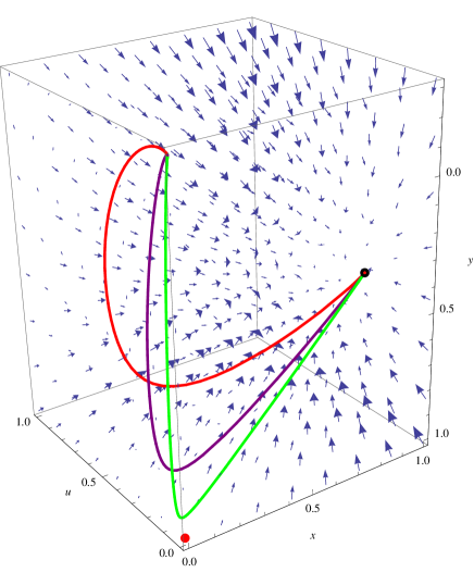
Figure 1: Some orbits in the phase space for the choice ($\zeta_{0}$, $\gamma_{de}$, $\alpha$)=($0.098$, $0.2$, $0.12$). This parameter election guarantee the saddle behavior of the pure DM dominated solution $P_{2a}$ (red point) and the late time attractor nature of $P_{3a}$, black point. Because of the nonzero value of $\zeta_{0}$ the early time unstable solution corresponds to a wrong RDE represented by blue point.

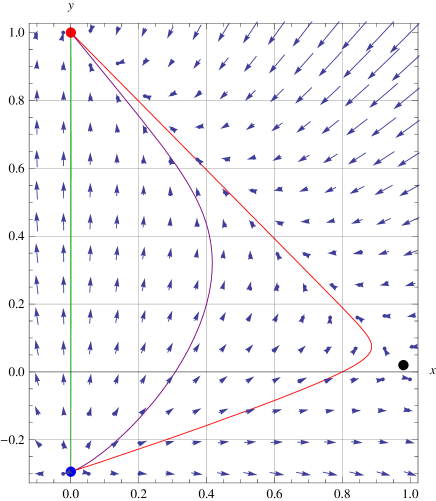
Figure 2: Some orbits in the phase space for the choice ($\zeta_{0}$, $\gamma_{de}$, $\alpha$)=($0.098$, $1.1$, $-0,1$). This parameter election guarantee the existence of the saddle critical point $P_{2c}$ and at the same time changes the dynamics of the phase portrait: now the late time attractor is the DM dominated solution $P_{2a}$ (red point) and the scaling solution between DM and DE, $P_{3a}$ (black point), display a saddle type behavior. As Table 2 shown, under this parameter choice $P_{3a}$ is contained, as a particular case, in $P_{2c}$. Because of the nonzero value of $\zeta_{0}$ the early time unstable solution corresponds to a wrong RDE represented by the blue point.

III.2 Cosmology evolution from critical points

According to our complete cosmological dynamics criterion, one of the critical points of any physically viable model should correspond to a RDE at early enough times, and this point should be an unstable point; the unstable nature of this critical point guarantees that it can be the source of any orbits in the phase space. The only two possible candidates so far in our model are points $P_{1a}$ and $P_{1c}$. Both cases require $-1\ll\zeta_{0}\leq 0$ in order to be a true RDE point, but such condition means a null contribution of bulk viscosity ($\zeta_{0}=0$), or else contradiction with the LSLT. Thus, we must conclude that no critical point exists in the model that can represent a RDE.

On the other hand, the evolution of the Universe requires the existence of a long enough matter dominated epoch, in which DM and baryons can be the dominant components. In our system, we need to look carefully at critical points $P_{2}$ to search for an appropriate candidate to be an unstable critical point dominated by the matter components.

In order to be in line with observations is better to avoid those initial conditions that lead orbits to approach point $P_{2a}$, as it does not permit the presence of baryons and its effective EOS is negative, but it represents a point dominated solely by DM. Points $P_{2b}$ and $P_{2d}$ must also be discarded, as their existence always requires a null value of the viscosity coefficient, and $P_{2d}$ even requires a null interaction between DM and DE.

The only possibility seems to be point $P_{2c}$, as long as observations could allow the presence of an early DE contribution to the energy density of the Universe. In such a case, the value of the viscosity coefficient $\zeta_{0}$ would have to be finely adjusted. Unfortunately, as we showed in the previous discussion, this critical point requires a non realistic DE component with EOS $w_{de}>0$ ($\gamma_{de}>1$) in one case, and violation of the LSLT through a negative value of the bulk viscosity ($\zeta_{0}<0$) in the other.

Finally, we must get, as a possibility to alleviate the coincidence problem of DE, a scaling solution with a nearly constant ratio between the energy densities of DM and DE at late times, which should in turn correspond to a stable critical point; the only one at hand in our system that could fulfill those expectations is $P_{3a}$. For the allowed values of $\zeta_{0}$, this point represents a scaling solution between the DE and DM components in the existence regions, and also admits a pure DE domination solution if only $\alpha=-\zeta_{0}$ ($\gamma\neq 1$). The required presence of the bulk viscosity limits the possibility of choosing initial condition that lead orbits to connect MDE to DM-DE scaling solution to the following possibilities:

• Orbits that connect $P_{2a}$ with $P_{3a}$. Despite the stable and accelerated nature of the scaling solution $P_{3a}$, it is not possible to recover the RDE and MDE as previously discussed. In Fig. 1 are shown some numerical integration of the autonomous system (7a-7c), for the interaction function (17) with ($\zeta_{0}$, $\gamma_{de}$, $\alpha$)=($0.098$, $0.2$, $0.12$). The orbits reveal that the $P_{3a}$ solution is the future attractor whereas the wrong RDE ($P_{1}$) is the past attractor.

• Orbits that connect $P_{2c}$ with $P_{3a}$. The existence conditions of both critical points (see Table 2) also implies that DM-DE scaling solution mimics the behavior of pressureless matter ($w_{eff}=0$). In the same region, this solution is not accelerated ($q=\frac{1}{2}$) being impossible to explain the late-time behavior of the Universe. This result rules out those initial conditions leading to orbits connecting both critical points. Fig. 2 shows some example orbits in the $x-y$ plane.

Unlike the above cases, the presence of non-null bulk viscosity entails no problem for a successful late-time accelerated evolution of the Universe but is impossible to recover a well behaved picture of the whole history of the Universe without be at variance with the LSLT. The simultaneous presence of interaction between DM and DE and bulk viscosity results in a very restrictive condition for the model.

IV Cosmological constraints

We now proceed to constrain the values of $(\zeta_{0},\gamma_{\rm de},\alpha)$, compute their confidence intervals, and calculate their best estimated values, as we compare with different cosmological observations that measure the expansion history of the Universe. For future reference, we write here an explicit expression for the normalized Hubble parameter, which is an exact result for the model (1):

$$E^{2}(z)=\Omega_{\rm r0}(1+z)^{4}+\Omega_{\rm b0}(1+z)^{3}+\\ +\Omega_{\rm de0}(1+z)^{3(\gamma_{\rm de}+\alpha)}+\hat{\Omega}_{\rm dm}(z)\,,$$ (19)

where $E(z)\equiv H(z)/H_{0}$, and the cumbersome formula for $\hat{\Omega}_{\rm dm}(z)$ is given in Eq. (43) of Appendix A, where all detailed calculations can be found.

IV.1 Cosmological data and $\chi^{2}$-functions

To perform all numerical analysis we take, for the baryon and radiation components (photons and relativistic neutrinos), the values of $\Omega_{b0}=0.0458$Komatsu et al. (2011), and $\Omega_{r0}=0.0000766$, respectively, where the latter value is computed from the expressionKomatsu et al. (2009)

$$\Omega_{\rm r0}=\Omega_{\gamma 0}(1+0.2271N_{\rm eff})\,.$$ (20)

Here, $N_{\rm eff}=3.04$ is the standard number of effective neutrino speciesKomatsu et al. (2011); Reid et al. (2010), and $\Omega_{\gamma 0}=2.469\times 10^{-5}h^{-2}$ corresponds to the present-day photon density parameter for a temperature of $T_{\rm cmb}=2.725$ KKomatsu et al. (2011), with $h$ the dimensionless Hubble constant: $h\equiv H_{0}/(100\mathrm{km/s/Mpc})$.

IV.1.1 Type Ia Supernovae

The luminosity distance $d_{L}$ in a spatially flat FRW Universe is defined as

$$d_{L}(z,\gamma_{\rm de},\alpha,\zeta_{0})=\frac{c(1+z)}{H_{0}}\int_{0}^{z}\frac{dz^{\prime}}{E(z^{\prime})}$$ (21)

where $c$ corresponds to the speed of light in units of $\mathrm{km/sec}$. The theoretical distance moduli $\mu^{t}$ for the $k$ - th supernova at a distance $z_{k}$ is given by

$$\mu^{t}(z,\gamma_{\rm de},\alpha,\zeta_{0})=5\log\left[\frac{d_{L}(z)}{\rm Mpc}\right]+25\,.$$ (22)

Hence, the $\chi^{2}$-function for the SNe is defined as

$$\chi^{2}_{\rm SNe}(\gamma_{\rm de},\alpha,\zeta_{0})\equiv\sum_{k=1}^{n}\left(\frac{\mu^{t}(z_{k},\gamma_{\rm de},\alpha,\zeta_{0})-\mu_{k}}{\sigm ạ_{k}}\right)^{2}\,,$$ (23)

where $\mu_{k}$ is the observed distance moduli of the $k$-th supernova, with a standard deviation of $\sigma_{k}$ in its measurement.

For our case, $n=580$, as we are using the type Ia supernovae (SNe Ia) in the Union2.1 data set of the Supernova Cosmology Project (SCP), which is composed of $580$ SNe Ia Suzuki et al. (2012). We have considered a flat prior probability distribution function to marginalize $H_{0}$ (i.e., it is not assumed any particular value of $H_{0}$).

IV.1.2 Cosmic Microwave Background Radiation

We use the shift parameter $R$ reported in Table 9 ofKomatsu et al. (2011), that is defined as

$$R=\frac{H_{0}\sqrt{\Omega_{\rm m0}}}{c}(1+z_{*})D_{A}(z_{*})\,,$$ (24)

where $\Omega_{\rm m0}$ is the present value of the density parameter of the all pressureless matter in the Universe, i.e. $\Omega_{\rm m0}=\Omega_{\rm b0}+\Omega_{\rm dm0}$, and $D_{A}$ is the proper angular diameter distance given by

$$D_{A}(z)=\frac{c}{(1+z)H_{0}}\int^{z}_{0}\frac{dz^{\prime}}{E(z^{\prime})}\,,$$ (25)

in a spatially flat Universe. We then define a $\chi^{2}$-function as

$$\chi^{2}_{\rm R-CMB}(\gamma_{\rm de},\alpha,\zeta_{0})\equiv\left(\frac{R-R_{\rm obs}}{\sigma_{R}}\right)^{2}\,,$$ (26)

where $R_{\rm obs}=1.725$ is the observed value of the shift parameter, and $\sigma_{R}=0.018$ is its standard deviation (cf. Table 9 ofKomatsu et al. (2011)).

SNe
Model	$\gamma_{\rm de}$	$\alpha$	$\zeta_{0}$	$\chi^{2}_{{\rm min}}$	$\chi^{2}_{{\rm d.o.f.}}$	DE	Energy Transfer	LSLT	CCD
I	$0^{*}$	$-0.0132^{+0.22}_{-0.37}$	$0.0017^{+0.097}_{-0.075}$	562.223	0.972	$\Lambda$	DE $\leftarrow$ DM	✓	✗
II	$-0.0011^{+0.1}_{-0.11}$	$-0.0086^{+0.1}_{-0.11}$	$0^{*}$	562.224	0.972	Phantom	DE $\leftarrow$ DM	✓	✓
III	$-0.0040\pm{0.14}$	$\alpha=\zeta_{0}$	$-0.0026^{+0.035}_{-0.032}$	562.224	0.972	Phantom	DE $\leftarrow$ DM	✗	✗
IV	$-0.0052\pm{0.18}$	$0^{*}$	$-0.0037^{+0.055}_{-0.051}$	562.225	0.972	Phantom	None	✗	✗
$H(z)$
I	$0^{*}$	$-0.632^{+0.56}_{-1.17}$	$0.193^{+0.14}_{-0.15}$	8.111	0.737	$\Lambda$	DE $\leftarrow$ DM	✓	✗
II	$-0.1976^{+0.13}_{-0.15}$	$-0.0127^{+0.07}_{-0.09}$	$0^{*}$	8.046	0.731	Phantom	DE $\leftarrow$ DM	✓	✓
III	$-0.199^{+0.15}_{-0.16}$	$\alpha=\zeta_{0}$	$-0.0033\pm 0.022$	8.049	0.731	Phantom	DE $\leftarrow$ DM	✗	✗
IV	$-0.2006^{+0.16}_{-0.17}$	$0^{*}$	$-0.00466^{+0.033}_{-0.031}$	8.051	0.731	Phantom	None	✗	✗
SNe + CMB + BAO + $H(z)$
I	$0^{*}$	$0.0324^{+0.024}_{-0.025}$	$-0.0085\pm 0.005$	572.766	$0.965$	$\Lambda$	DE $\to$ DM	✗	✗
II	$-0.0628^{+0.047}_{-0.049}$	$-0.0112^{+0.012}_{-0.013}$	$0^{*}$	574.219	0.968	Phantom	DE $\leftarrow$ DM	✓	✓
III	$-0.0589^{+0.043}_{-0.045}$	$\alpha=\zeta_{0}$	$-0.0023\pm 0.0019$	573.618	0.967	Phantom	DE $\leftarrow$ DM	✗	✗
IV	$-0.0573^{+0.043}_{-0.044}$	$0^{*}$	$-0.0028\pm 0.002$	573.522	0.967	Phantom	None	✗	✗
V	$(-6.04\times 10^{-9})\pm 0.05$	$0.028\pm 0.03$	$-0.008\pm 0.006$	571.199	0.965	Phantom	DE $\to$ DM	✗	✗
$\Lambda$CDM	$0^{*}$	$0^{*}$	$0^{*}$	573.572	0.970	$\Lambda$	None	✓	✓

Table 5: Marginal best estimated values of the parameters $(\gamma_{\rm de},\alpha,\zeta_{0})$ for the different models discussed in the text; notice that the DM barotropic index is that of a dust fluid for all cases, $\gamma_{\rm DE}=1$. The asterisk superscript indicates the cases when the zero value of one of the parameter was assumed a priori. The top (middle) table only considers SNe ($H(z)$) observations, whereas the bottom table correspond to the use of the combined SNe + CMB + BAO + $H(z)$ data sets together, see Sec. IV. The fourth and fifth columns correspond to the minimum value of the $\chi^{2}$ function, $\chi^{2}_{\rm min}$, and the $\chi^{2}$ by degrees of freedom, $\chi^{2}_{\rm d.o.f.}$, respectively. The latter is defined as $\chi^{2}_{\rm d.o.f.}=\chi^{2}_{\rm min}/(n-p)$, where $n$ is the number of data and $p$ the number of free parameters. The next-to-last row (Model V) corresponds to best estimates of the three parameters $(\gamma_{\rm de},\alpha,\zeta_{0})$ computed simultaneously. $H_{0}$ was marginalized assuming a flat prior distribution. The last row, with $(\gamma_{\rm de}=0,\alpha=0,\zeta_{0}=0)$ corresponds to the value that we obtain for the $\Lambda$CDM model, using the same procedure and data sets, in order to compare our results. According to the value $\chi^{2}_{\rm d.o.f.}$, we find that all our cases fit the data sets as well as $\Lambda$CDM does. Last columns indicate the type of DE, the energy transfer direction, the consistency with the Local Second Law of Thermodynamics (LSLT, Eq. (5)), and with a complete cosmological dynamics (CCD) as discussed in Sec. II.2. See Figs. 3 to 6 for their corresponding confidence intervals, and the text for more details.

IV.1.3 Baryon Acoustic Oscillations

We use the baryon acoustic oscillation (BAO) data from the SDSS 7-years release Percival et al. (2010), expressed in terms of the distance ratio $d_{z}$ at $z=0.275$, which is defined as

$$d_{0.275}\equiv\frac{r_{s}(z_{d})}{D_{V}(0.275)}\,,$$ (27)

where $r_{s}(z)$ corresponds to the comoving sound horizon given by

$$r_{s}(z)=\frac{c}{\sqrt{3}}\int_{0}^{1/(1+z)}\frac{da}{a^{2}H(a)\sqrt{1+(3\Omega_{\rm b0}/4\Omega_{\gamma 0})a}}\,.$$ (28)

As mentioned above, we take the following actual values of the density parameters: $\Omega_{\gamma 0}=2.469\times 10^{-5}h^{-2}$ for photons, and $\Omega_{b0}=0.02255h^{-2}$ for baryonsKomatsu et al. (2011). And $z_{d}$ is the redshift at the baryon drag epoch computed from the fitting formulaEisenstein and Hu (1998)

$$z_{d} = 1291\frac{(\Omega_{\rm m0}h^{2})^{0.251}}{1+0.659(\Omega_{\rm m0}h^{2})^{0.828}}\left[1+b_{1}(\Omega_{\rm m0}h^{2})^{b_{2}}\right]\,,$$ (29a)

$$b_{1} = 0.313(\Omega_{\rm m0}h^{2})^{-0.419}\left[1+0.607(\Omega_{\rm m0}h^{2})^{0.674}\right]\,,$$ (29b)

$$b_{2} = 0.238(\Omega_{\rm m0}h^{2})^{0.223}\,.$$ (29c)

For a flat Universe, $D_{V}(z)$ is defined as

$$D_{V}(z)=c\left[\left(\int_{0}^{z}\frac{dz^{\prime}}{H(z^{\prime})}\right)^{2}\frac{z}{H(z)}\right]^{1/3}\,.$$ (30)

It contains the information of the visual distortion of a spherical object due the non-Euclidianity of the FRW spacetime. Parameter $d_{0.275}$ contains the information of the other two pivots, $d_{0.2}$, and $d_{0.35}$, that are usually used by other authors, with a precision of $0.04\%$ Percival et al. (2010).

The $\chi^{2}$ function for BAO is then given by

$$\chi^{2}_{\rm BAO}(\gamma_{\rm de},\alpha,\zeta_{0})\equiv\left(\frac{d_{0.275}-d_{0.275}^{\rm obs}}{\sigma_{d}}\right)^{2}\,,$$ (31)

where $d_{0.275}^{\rm obs}=0.139$ is the observed value, and $\sigma_{d}=0.0037$ is its standard deviationPercival et al. (2010).

IV.1.4 Hubble expansion rate

For the Hubble parameter we use the $13$ available data; $11$ data come from Table 2 in Stern et al. (2010)Stern et al. (2010), and other 2 from Gaztanaga et al. (2010)Gaztanaga et al. (2009): $H(z=0.24)=79.69\pm 2.32$ and $H(z=0.43)=86.45\pm 3.27$ km/s/Mpc. For the present value of the Hubble parameter, we take the value reported by Riess et al (2011)Riess et al. (2011): $H(z=0)\equiv H_{0}=73.8\pm 2.4$ km/s/Mpc. The $\chi^{2}$ function is

$$\chi^{2}_{\rm H}(\gamma_{\rm de},\alpha,\zeta_{0})=\sum_{i}^{13}\left(\frac{H(z_{i})-H_{i}^{\rm obs}}{\sigma_{H}}\right)^{2}\,,$$ (32)

where $H(z_{i})$ is the theoretical value predicted by the model, and $H_{i}^{\rm obs}$ is the observed value with a standard deviation $\sigma_{H}$.

IV.2 Observational constraints

Finally, with each of the $\chi^{2}$-functions defined above we construct the total $\chi^{2}$-function given by

$$\chi^{2}=\chi^{2}_{\rm SNe}+\chi^{2}_{\rm CMB}+\chi^{2}_{\rm BAO}+\chi^{2}_{\rm H}.$$ (33)

We minimize this function with respect to the parameters $(\gamma_{\rm de},\alpha,\zeta_{0})$ to compute their best estimated values and confidence intervals.

There are four special cases we will discuss here, whose parameters are described and estimated in Table 5, and in the confidence intervals (CI) in Figs. 3, 4, 5, and 6.

Some general comments are in turn before the detailed explanation of the different models. First, we have noticed, for the quantities reported in Table 5, that there is a qualitative change in the models if only the low-redshift data sets are taken into account; in our case, these data sets are those of the supernovae (SNe) and the Hubble parameter ($H(z)$). Such change is particularly acute in the case of the bulk viscosity $\zeta_{0}$: it is consistently positive definite whenever the interaction parameter $\alpha$ is set free, like in Model I. If $\alpha$ is fixed to be equal to $\zeta_{0}$, or to have a null value, then the bulk viscosity is negative definite, like in Models III and IV.

But right the opposite happens if high-redshift measurements are included in the analysis: all models consistently point out to a negative value of the bulk viscosity whenever it is freely fitted, like in Models I, III, and IV. This means, actually, that all models with bulk viscosity as a free parameter are at variance with the LSLT when they are fitted to the sample set of cosmological observations.

Our second general comment is that none of the models is consistent with our so-called statement of complete cosmological dynamics presented and discussed in Sec. II.2. The main reason being that we cannot recover an appropriate RDE at early times. One must notice, though, that our data sets cannot cover high enough redshifts in order to properly sample the early RDE of the Universe, but it is nonetheless significant that the estimated values of the free parameters already indicate a non-recovery of an RDE. Such a difficulty was already observed in models with bulk viscosityAvelino et al. (2013); Velten and Schwarz (2012) , but it has not been sufficiently remarked in models with a DM-DE interactionChimento et al. (2009); Quartin et al. (2008); Caldera-Cabral et al. (2009).

One last comment regards that of the nature of DE in all models: we have consistently found that phantom DECaldwell (2002); *Scherrer:2004eq is slightly favored by all data sets whenever the DE EOS is freely varied, and that in most of the models an energy transfer from DM to DE is preferred.

IV.2.1 Model I

Model I corresponds to $\gamma_{\rm DE}=0$, whereas $\alpha$ and $\zeta_{0}$ are free parameters; that is, this case corresponds to a DE-DM interacting model, in which DM is a dust fluid with bulk viscosity, and DE is a cosmological constant, see for instanceKremer and Sobreiro (2012); Jamil and Farooq (2009); Adabi et al. (2012) and references therein for similar models.

According to the values presented in Table 5 and in Fig. 3, the bulk viscosity is positive for low-redshift data sets, but it takes small negative values when the full data set is considered. However, we must recall that $\zeta_{0}<0$ is forbidden by the LSLT, see Eq. (5), and because of this Model I would then be ruled out with at least $68\%$ of probability ($1\sigma$). We notice that there is a slight preference for small but positive values of $\alpha$, i.e, from the figure 3 we see that the $68\%$ contour region lies in the positive region for $\alpha$. Finally, the CI for $(\zeta_{\rm 0},\alpha)$ parameters lie almost completely in a region that is not consistent with a well behaved cosmology defined by the dynamical system analysis in Sec. II.2, because none of the critical points $P_{1a}$, $P_{2a}$ or $P_{1c}$, see Table 2, is a suitable point for a RDE; this fact then adds for the ruling out of this model.

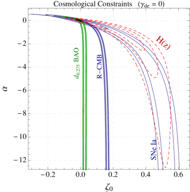
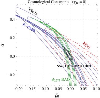
Figure 3: Confidence intervals (CI) for Model I: $(\zeta_{\rm 0},\alpha)$ as free parameters, and $\gamma_{\rm DE}=0$. The CI shown correspond to $68.3\%$, $95.4\%$ and $99.7\%$ of confidence level. We notice from this figure that, with $99.7\%$ of confidence, and using the combined SNe + CMB + BAO + $H(z)$ data sets together, the values lie on the regions $-0.029<\zeta_{\rm 0}<0.011$ and $-0.062<\alpha<0.11$, when $(\zeta_{0},\alpha)$ are constrained simultaneously. The marginal best estimated values for each parameter individually are $\zeta_{\rm 0}=-0.0085\pm 0.005$, and $\alpha=0.0324^{+0.024}_{-0.025}$, where the errors are given to $68.3\%$ of confidence, see also Table 5. (Right) Zoom in of the CI around the best estimated values. The bulk viscosity is constrained to small negative values; however, $\zeta_{0}<0$ is forbidden by the LSLT, and then Model I is ruled out with a $68\%$ of probability ($1\sigma$). We notice that there is a slight preference for small but positive values of $\alpha$. Finally, the CI for $(\zeta_{\rm 0},\alpha)$ parameters lie almost completely in a region that is not consistent with a well behaved cosmology defined by the dynamical system analysis, and then Model I must be considered to be ruled out.

IV.2.2 Model II

Model II corresponds to $\zeta_{0}=0$, whereas $\gamma_{\rm DE}$ and $\alpha$ are free parameters; that is, it corresponds to a purely DM-DE interacting model, see for instanceQuartin et al. (2008); Caldera-Cabral et al. (2009); *Caldera-Cabral2010; Cruz et al. (2012) and references therein. By definition, this model is in agreement with the LSLT.

Both parameters $(\gamma_{\rm de},\alpha)$ are close to zero, but phantom DE is slightly favored, $(\gamma_{\rm DE}<0)$ at about $68.3\%$ (1$\sigma$), as also is $\alpha<0$, which corresponds to energy transfer from DM to DE. In both region, as shown in Table 2, the model describes a complete cosmological dynamics since is possible to choose initial conditions that lead orbits to connect $P_{1a}$$\rightarrow$ $P_{2b}$$\rightarrow$$P_{3a}$.

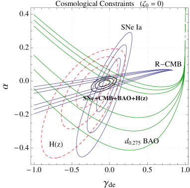
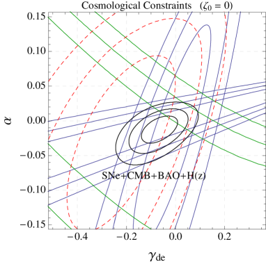
Figure 4: Confidence intervals for Model II (DM-DE interacting model without bulk viscosity): $(\gamma_{\rm de},\alpha)$ as free parameters, and $\zeta_{\rm 0}=0$. The CI correspond to $68.3\%$, $95.4\%$ and $99.7\%$ of confidence level. We notice that, with $99.7\%$, and using the combined SNe + CMB + BAO + $H(z)$ data sets together, the values lie on the regions $-0.25<\gamma_{\rm de}<0.10$ and $-0.065<\alpha<0.028$ , when $(\gamma_{\rm de},\alpha)$ are constrained simultaneously. The marginal best estimated values for each parameter individually are $\gamma_{\rm de}=-0.0628^{+0.047}_{-0.049}$, and $\alpha=-0.0112^{+0.012}_{-0.013})$, where the errors are given to $68.3\%$ of confidence, see also Table 5. (Right) Zoom in of CI around the best estimated values. Both parameters $(\gamma_{\rm de},\alpha)$ are close to zero, but phantom DE is slightly favored, $\gamma_{\rm DE}<0$, at about $68.3\%$ (1$\sigma$), as also is $\alpha<0$, which corresponds to energy transfer from DM to DE.

IV.2.3 Model III

Model III corresponds to $\alpha=\zeta_{0}$, whereas $\gamma_{\rm DE}$ and $\zeta_{0}$ are free parameters; that is, this case corresponds to an interacting bulk viscous DM-DE model, where the interacting parameter is directly proportional to the bulk viscosity. A related model was studied by Kremer and SobreiroKremer and Sobreiro (2012) where they assume $\alpha=-\zeta_{0}$.

We find interesting that the CI’s presented in Fig. 5 are almost identical to those of Model II (for $\alpha=0$), see Sec. IV.2.2 and Fig. 4, suggesting that the value of the bulk viscosity and the nature of the DE component in this model is insensitive to the assumption of the DM-DE interaction. This model is not compatible with a RDE, as Table  2 shown. In addition, is not possible to recover a true MDE since only $P_{2a}$ is fulfilled, namely a pure DM domination with a null contribution of baryonic matter. Regardless of the initial conditions, $P_{3a}$ is the only possible late time attractor of Model III, but, as Table 5 shows, observations favor negative values for $\alpha$ (and hence for $\zeta_{0}$) and, for those negative values $P_{3a}$ does not belong to the phase space (9) of the model. Thus, the model is ruled out because it is neither compatible with a complete cosmological dynamics nor with the LSLT.

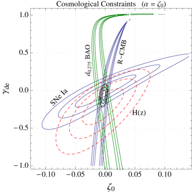
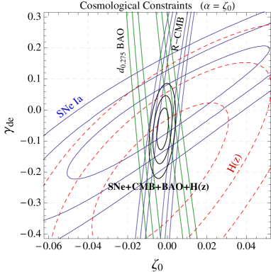
Figure 5: Confidence intervals (CI) for Model III: $(\zeta_{\rm 0},\gamma_{\rm de})$ as free parameters, and $\alpha=\zeta_{\rm 0}$. The CI shown correspond to $68.3\%$, $95.4\%$ and $99.7\%$ of confidence level. We notice that, with $99.7\%$, and using the combined SNe + CMB + BAO + $H(z)$ data sets together, the values lie in the regions $-0.011<\zeta_{\rm 0}<0.005$ and $-0.22<\gamma_{\rm de}<0.09$, when $(\zeta_{\rm 0},\gamma_{\rm de})$ are constrained simultaneously. The marginal best estimated values for each parameter individually are $(\zeta_{\rm 0}=-0.0023\pm 0.0019,\gamma_{\rm de}=-0.0589^{+0.043}_{-0.045})$, where the errors are given to $68.3\%$ of confidence, see also Table 5. (Right) Zoom in of the CI around the best estimated values. We find interesting that the CI’s are almost identical to the case $\alpha=0$ (see Fig. 6), suggesting that the value of the bulk viscosity and the nature of the DE in this model is insensitive to the assumption of the interaction. However, this model must be considered to be ruled out because is at variance with the LSLT ($\zeta_{0}<0$) and is not consistent with a complete cosmological dynamics.

IV.2.4 Model IV

Model IV corresponds to $\alpha=0$, whereas $\gamma_{\rm DE}$ and $\zeta_{0}$ are free parameters; that is, it corresponds to a non-interacting DM-DE model, in which DM has bulk viscosity. See for instance Kremer and Devecchi (2003); Cataldo et al. (2005) and references therein.

From the CI of the joint SNe + CMB + BAO + $H(z)$ datasets we find that the bulk viscosity is constrained again to small values and mainly in the negative region, with almost $68\%$ of probability ($1\sigma$), that is in tension with the LSLT and our statement of a complete cosmological dynamics. On the other hand, we find that values of $\gamma_{\rm de}<0$ are preferred by the observations with at least $68\%$ of probability, corresponding to phantom DE.

IV.2.5 Model V and $\Lambda$CDM

Model V corresponds to the case in which all parameters are freely varied simultaneously, and as such is our most general case. As in previous cases, we find again that phantom DE is slightly preferred, as is also the energy transfer from DE to DM. However, the final output is not compatible with the LSLT nor with a complete cosmological dynamics; the latter mainly because a proper RDE cannot be recover at early time.

Just for comparison, we have also fitted the $\Lambda$CDM model to the same data and using the procedure; notice that this model is also our null-hypothesis case, as it is recovered if all parameters are given null values. Interestingly enough, the good of fitness of our models is as good as that of $\Lambda$CDM, a fact that points out that the used data sets are not powerful enough to differentiate the models; this is why we had to consider other constraints from the theoretical point of view, like that of the LSLT in Eq. (5), and the complete cosmological dynamics reviewed in Sec. III.2.

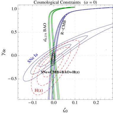
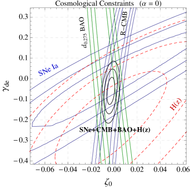
Figure 6: Confidence intervals (CI) for Model IV: $(\zeta_{0},\gamma_{\rm de})$ as free parameters, and $\alpha=0$. The CI correspond to $68.3\%$, $95.4\%$ and $99.7\%$ of confidence level. We notice from this figure that, with $99.7\%$, and using the combined SNe + CMB + BAO + $H(z)$ data sets together, the values lie on the regions $-0.011<\zeta_{0}<0.005$ and $-0.22<\gamma_{\rm de}<0.085$, when $(\zeta_{0},\gamma_{\rm de})$ are constrained simultaneously. The marginal best estimated values for each parameter individually are $\zeta_{\rm 0}=-0.0028\pm 0.002$, and $\gamma_{\rm de}=-0.0573^{+0.043}_{-0.044})$, where the errors are given to $68.3\%$ of confidence, see also Table 5. (Right) Zoom in of the CI around the best estimated values. The bulk viscosity is constrained again to small values and mainly in the negative region, with almost $68\%$ of probability ($1\sigma$), that is in tension with the LSLT and with the requirement of a well behaved cosmology from the dynamical system analysis. So, Model IV is ruled out with almost $1\sigma$. On the other hand, we find that values of $\gamma_{\rm DE}<0$ are preferred by the observations with a $68\%$ of probability, corresponding to a phantom dark energy.

V Discussion and Conclusions

In the present work we studied, in general terms, a cosmological model that includes DM with bulk viscosity, an interaction term between DM and DE, and a free barotropic equation of state $p=(\gamma_{\rm de}-1)\rho_{\rm de}$. The dissipation in the DM component was characterized by a bulk viscosity $\zeta$ directly proportional to the expansion rate of the Universe, i.e., $\zeta=H\zeta_{0}/(8\pi G)$, where $\zeta_{0}$ is a dimensionless constant. Another important assumption was that, except the DM, all matter components are represented by perfect fluids, which in itself constraints the type of DE that are affected by our analysis.

First of all, we performed a detailed dynamical system analysis of the model in order to investigate its asymptotic evolution and behavior. In addition, we demanded that our model must follow what we called a complete cosmological dynamics, namely: the existence of a viable RDE and MDE prior to a late-time acceleration stage; these three different eras have to be present in any model of physical interest. The imposition of this requirement rules out any model with a bulk viscosity in the DM sector. This results from the fact that the bulk viscosity needs to be negative definite in order to have standard RDE and MDE, but that is not possible if we are to believe in the LSLT. However, a negative definite bulk viscosity is compatible with the speed up of the Universe at low redshifts, which actually was one of the appealing aspects of these type of models.

For purposes of illustration, we have applied our general results to the specific interaction function: $Q=3\alpha\rho_{\rm de}H$, where the parameter $\alpha$ quantifies the strength and direction of the DM-DE interaction. As said before, we found that the bulk viscosity parameter was the troublesome one, and that we could accommodate a complete cosmological dynamics as long as $\zeta_{0}=0$.

Also, we tested the model using cosmological observations to estimate the free parameters and set constraints on them. The three parameters ($\gamma_{\rm de},\alpha,\zeta_{0}$) allowed us to have a very rich diversity of possible models to study, from purely interacting models ($\zeta_{0}=0$), to purely viscous models ($\alpha=0$), and even the case of $\Lambda$CDM, which then acted as our null hypothesis ($\zeta_{0}=0=\alpha$).

Whenever we tested a model with a non-null bulk viscosity, we found that a negative value of it was preferred, with at least 1$\sigma$ of confidence level. This result is a drawback of the model, given that it is in tension with the LSLT that reads $\zeta_{0}>0$ for our model. It should be said, though, that such a result was obtained if high-redshift data was included in the analysis. Actually, low-redshift data seems to favor a positive definite value of the bulk viscosity, but that would have lead us to wrong conclusions about the viability of the model. As for the interaction parameter $\alpha$, we found that in general the data favor a negative value, indicating an energy transfer from the DM to DE.

On the other hand, it is interesting to notice that using the cosmological observations we consistently found negative values of the barotropic index $\gamma_{\rm de}$, suggesting a phantom nature for the DE fluid that is in agreement with recent resultsAde et al. (2013), even though such a setup is troublesome from the theoretical point of view (like in the violation of the null energy condition $\rho+p\geq 0$).

We computed also the $\chi^{2}_{\rm d.o.f.}$ of all the models, and found that the goodness-of-fit to the data were equally good for all of them. This fact seems to indicate that the inclusion of new free parameters did not significantly improve the viability of the models, nor did it help to distinguish them from the null hypothesis represented by the concordance $\Lambda$CDM model.

*

Appendix A The Hubble parameter

Here, we give details about the calculation of the Hubble parameter, see Eq. (23), that is required in Sec. IV to compute the observational constraints.

The exact solutions of the conservation equations (1b), and (1c), are, respectively,

$$\rho_{\rm r}(a)=\rho_{\rm r0}/a^{4}\,,\quad\rho_{\rm b}(a)=\rho_{\rm b0}/a^{3}\,,$$ (34)

where $a$ is the scale factor, and the subscript zero labels the present values of the energy densities. If we take the interaction term $Q=3H\alpha\rho_{\rm de}$, the conservation equations (1d), and (1e) can be rewritten as

$$\dot{\rho}_{\rm dm}+3H\gamma^{e}_{\rm dm}\rho_{\rm dm}=0\,,\quad\dot{\rho}_{\rm de}+3H\gamma^{e}_{\rm de}\rho_{\rm de}=0\,,$$ (35)

where we have defined the effective barotropic indexes

$$\gamma^{e}_{\rm dm} = \gamma_{\rm dm}+(\gamma_{\rm de}-\gamma^{e}_{\rm de})\frac{\rho_{\rm de}}{\rho_{\rm dm}}-\frac{3H\zeta}{\rho_{\rm dm}}\,,$$ (36)

$$\gamma^{e}_{\rm de} = \gamma_{\rm de}+\alpha\,.$$ (37)

As all parameters are constant, we can integrate the equation of motion for the DE energy density, see Eq. (35) and obtain

$$\rho_{\rm de}(a)=\rho_{\rm de0}a^{-3(\gamma_{\rm de}+\alpha)}\,.$$ (38)

Hence, the barotropic index of DM, see Eq. (36), can be written as

$$\gamma^{e}_{\rm dm}=\gamma_{\rm dm}-\frac{1}{\rho_{\rm dm}}\left(\alpha\rho_{\rm de}+\zeta_{0}\frac{3H^{2}}{8\pi G}\right)\,.$$ (39)

With the help of the Friedmann constraint (1a), and the exact solutions of the energy densities, Eq. (39) can be finally rewritten as

$$\gamma^{e}_{\rm dm}=\gamma_{\rm dm}-\frac{1}{\rho_{\rm dm}}\left[\zeta_{0}\left(\frac{\rho_{\rm r0}}{a^{4}}+\frac{\rho_{\rm b0}}{a^{3}}+\rho_{\rm dm}\right)+\right.\\ \left.+\frac{\rho_{\rm de0}}{a^{3(\gamma_{\rm de}+\alpha)}}(\alpha+\zeta_{0})\right]\,,$$ (40)

and then the equation of motion (35) for the DM energy density becomes

$$\dot{\rho}_{\rm dm} = -3H\left[\gamma_{\rm dm}\rho_{\rm dm}\vphantom{\frac{\rho_{r0}}{a^{4}}}-\zeta_{0}\left(\frac{\rho_{\rm r0}}{a^{4}}+\frac{\rho_{\rm b0}}{a^{3}}+\rho_{\rm dm}\right)\right.$$ (41)

$$\left.-\frac{\rho_{\rm de0}}{a^{3(\gamma_{\rm de}+\alpha)}}(\alpha+\zeta_{0})\right]\,.$$

Next, we take the dimensionless density parameters for all matter components, $\Omega_{i0}\equiv\rho_{i0}/\rho^{0}_{\rm crit}$ and $\hat{\Omega}_{\rm dm}\equiv\rho_{\rm dm}/\rho^{0}_{\rm crit}$, where $\rho_{\rm crit}^{0}\equiv 3H^{2}_{0}/(8\pi G)$ is the present critical density; thus, Eq.  (41) becomes

$$\frac{(1+z)}{3}\frac{d\hat{\Omega}_{\rm dm}}{dz}-\hat{\Omega}_{\rm dm}(\gamma_{\rm dm}-\zeta_{0})+\Omega_{\rm de0}(\alpha+\zeta_{0})(1+z)^{3(\gamma_{\rm de}+\alpha)}+\zeta_{0}(1+z)^{3}\left[\Omega_{\rm r0}(1+z)+\Omega_{\rm b0}\right]=0\,.$$ (42)

where $z$ is the redshift, which is related to the scale factor through $a=1/(1+z)$. The analytical solution of Eq. (42) is:

$$\hat{\Omega}_{\rm dm}(z)=\frac{1}{(1+z)^{3\zeta_{0}}(1+3\zeta_{0})(\alpha+\gamma_{\rm de}+\zeta_{0}-1)}\left\{3\zeta_{0}^{2}\left[(\Omega_{\rm b0}+\Omega_{\rm dm0}+\Omega_{\rm r0}-1)(1+z)^{3(\alpha+\gamma_{\rm de}+\zeta_{0})}-\right.\right.\\ \left.-(1+z)^{3(1+\zeta_{0})}\left((1+z)\Omega_{\rm r0}+\Omega_{\rm b0}\right)+(1+z)^{3}\right]+\alpha(3\zeta_{0}+1)(\Omega_{\rm b0}+\Omega_{\rm dm0}+\Omega_{\rm r0}-1)(1+z)^{3(\alpha+\gamma_{\rm de}+\zeta_{0})}+\\ +\zeta_{0}\left[(\Omega_{\rm b0}+\Omega_{\rm dm0}+\Omega_{\rm r0}-1)(1+z)^{3(\alpha+\gamma_{\rm de}+\zeta_{0})}+(1+z)^{3(1+\zeta_{0})}\left((2-3\gamma_{\rm de})\Omega_{\rm b0}-3(1+z)(\gamma_{\rm de}-1)\Omega_{\rm r0}\right)+\right.\\ \left.+(1+z)^{3}\left(3(\gamma_{\rm de}-1)(\Omega_{\rm b0}+\Omega_{\rm dm0})+(3\gamma_{\rm de}-4)\Omega_{\rm r0}+1\right)\right]+\alpha(1+z)^{3}\left[(1+z)^{3\zeta_{0}}\left(-3(1+z)\zeta_{0}\Omega_{\rm r0}-\right.\right.\\ \left.\left.\left.-(1+3\zeta_{0})\Omega_{\rm b0}\right)+3\zeta_{0}-\Omega_{\rm r0}+1\right]-(1+z)^{3}(\gamma_{\rm de}-1)\left[\Omega_{\rm b0}\left((1+z)^{3\zeta_{0}}-1\right)-\Omega_{\rm dm0}\right]\right\},$$ (43)

where we have set $\gamma_{\rm dm}=1$, and made use of the present Friedmann constraint $\Omega_{\rm de0}=1-\left(\Omega_{\rm r0}-\Omega_{\rm b0}-\Omega_{\rm dm0}\right)$.