Repulsive Interactions in Quantum Hall Systems as a Pairing Problem

Abstract

A subtle relation between Quantum Hall physics and the phenomenon of pairing is unveiled. By use of second quantization, we establish a connection between (i) a broad class of rotationally symmetric two-body interactions within the lowest Landau level and (ii) integrable hyperbolic Richardson-Gaudin type Hamiltonians that arise in $(p_{x}+ip_{y})$ superconductivity. Specifically, we show that general Haldane pseudopotentials (and their sums) can be expressed as a sum of repulsive non-commuting $(p_{x}+ip_{y})$-type pairing Hamiltonians. The determination of the spectrum and individual null spaces of each of these non-commuting Richardson-Gaudin type Hamiltonians is non-trivial yet is Bethe Ansatz solvable. For the Laughlin sequence, it is observed that this problem is frustration free and zero energy ground states lie in the common null space of all of these non-commuting Hamiltonians. This property allows for the use of a new truncated basis of pairing configurations in which to express Laughlin states at general filling factors. We prove separability of arbitrary Haldane pseudopotentials, providing explicit expressions for their second quantized forms, and further show by explicit construction how to exploit the topological equivalence between different geometries (disk, cylinder, and sphere) sharing the same topological genus number, in the second quantized formalism, through similarity transformations. As an application of the second quantized approach, we establish a “squeezing principle” that applies to the zero modes of a general class of Hamiltonians, which includes but is not limited to Haldane pseudopotentials. We also show how one may establish (bounds on) “incompressible filling factors” for those Hamiltonians. By invoking properties of symmetric polynomials, we provide explicit second quantized quasi-hole generators; the generators that we find directly relate to bosonic chiral edge modes and further make aspects of dimensional reduction in the Quantum Hall systems precise.

I Introduction

The study of strongly correlated phases of matter is a supremely challenging task, and yet has let to some of the most notable triumphs in condensed matter physics. A major route to success along these lines has been the identification of special points within a given phase of interest, where the Hamiltonian becomes somewhat tractable and leads to sufficiently simple ground and excited state wave functions, either through exact or approximate treatment, that nonetheless capture the essential universal features of the phase as a whole. The fractional Quantum Hall (FQH) regime harbors a wealth of examples of the latter kind. Indeed, in the presence of a strong magnetic field, powerful principles are known constraining the construction of successful trial wave functionslaughlin ; jain ; Moore as well as model Hamiltonians.Haldane Moreover, for many (though certainly not all) known trial wave functions describing various phases (or critical pointsgaffnian ) in the FQH regime, a local model Hamiltonian can be identified for which the wave function in question is an exact ground state. The identification of such parent Hamiltonians is usually greatly aided by special analytic properties of the underlying wave function. The primary example where this scheme of attack has been successful is the $\nu=1/3$ Laughlin state, whose parent Hamiltonian is the $V_{1}$ Haldane pseudopotential.Haldane ; Trugman For fermions, the latter can be regarded as the simplest local two-body interaction within the lowest Landau level (LLL).

Despite these powerful applications, the dependence on analytic wave function properties in the construction of Quantum Hall (QH) parent Hamiltonians also leads to severe inherent limitations. For one, many QH phases of fundamental interest, such as those described by hierarchyHaldane ; halperin or Jainjain composite fermion states, do not have known parent Hamiltonians. Moreover, as was recently argued by Haldane,Haldane2011 all information about the topological order of the ground states is encoded in the guiding center degrees of freedom only, whereas analytic properties of the wave function are due to the interplay of the latter with the particles’ dynamical momenta, which determine the structure of a given Landau level. This structure is arguable not essential for the topological quantum order of the QH fluid. Indeed, as we will review below, in a strong uniform magnetic field one may formulate the Hamiltonian dynamics of the electrons in a second-quantized “guiding-center only” language, which is stripped of the dynamical momenta entirely. As is well appreciated, QH physics is intimately tied to dimensional reduction which is similarly manifest in many other systems exhibiting topological orders. NO In the associated “guiding-center only” second quantized Hamiltonian (wherein the two spatial dimensions of the original QH problem in first quantization are replaced by a one-dimensional (1D) fermionic lattice of the angular momentum orbitals) this dimensional reduction becomes explicit and leads to a class of 1D lattice models which may be of interest in a more general context outside Landau-level physics (see Fig. 1). Specifically, this has been proposed recently for flat band solids with and without Chern numbers.Qi ; Scarola

For all the above reasons, it is desirable to understand the existing parent Hamiltonians of FQH model wave functions in the context of 1D lattice Hamiltonians, 1Dparent ; seidel ; berg ; Nakamura and most importantly the QH projected Hamiltonian in second quantized form. Due to technical difficulties that we will elaborate on below (see also Ref. zhou12, ), there currently seems to be very limited understanding of how the (quasi)-solvability of FQH parent Hamiltonians follows from its defining operator algebra in the 1D lattice or “guiding center” picture.

In this work, we aim to improve on the above situation. We expose a connection between the operator algebra defining the parent Hamiltonian of Laughlin QH states on the one hand, and another paradigmatic state of strongly correlated matter on the other, the superconductor. More precisely, we expose that a generic two-body interaction can be written as a direct sum of hyperbolic Richardson-Gaudin (RG) Hamiltonians in the strongly coupled repulsive regime. NuclPhysB Hyperbolic RG models represent a general class of exactly solvable pairing Hamiltonians which includes the $p_{x}+ip_{y}$ superconductor as a particular instance. Romb We use the fact that the latter (generally non-commuting) RG Hamiltonians are exactly solvable (by Bethe-Ansatz NuclPhysB ; Romb ) to characterize the individual non-trivial null spaces of these RG operators at a given filling $\nu$. The common null space of the latter is the corresponding Laughlin state. Thus, when expressed as a sum of RG Hamiltonians, the “frustration free” character of the system is underscored. A Hamiltonian is termed “frustration free” (or “quantum satisfiable”) whenever all of its null states are also null states of each of the individual terms (in our case, RG Hamiltonians) that form it. That is, the ground states of any individual RG Hamiltonian are globally consistent with the ground state null space of the full Hamiltonian. Frustration free Hamiltonians have recently been under intense study at the interface of condensed matter and quantum information theory. frustration_free We remark that while most frustration free Hamiltonians studied in the literature are sums of similar local Hamiltonians which merely operate on different sites (e.g., local Hamiltonians related to one another by lattice translations), those in the QH problem are richer; the RG Hamiltonians which form the full QH system that we consider are not strictly finite ranged. Thus, unlike in simple lattice models, the study of their eigenstates and eigenvalues is already a rich and non-trivial problem. We further explicitly note that the aforementioned strongly repulsive $(p_{x}+ip_{y})$-type RG Hamiltonians that we will study, which share conventional Laughlin states as their common ground states are notably very different from the far more exotic Pfaffian type states for other fillings and viable insightful links to superconductivity therein. Moore ; Read Our hope is that by understanding the common null space of all hyperbolic RG Hamiltonians we will be able to shed light on QH fluids with filling fractions $\nu$ other than those with Laughlin type ground states.

Aside from considerations regarding effective field theories, the QH problem seems to find its most common representation in a first quantized language of known (or guessed) ground states where properties of holomorphic functions can be elegantly employed. The second quantized formulation, on the other hand, sheds light on the algebraic structure of QH system and does not explicitly rely on prior knowledge of the form of the ground states. It further allows for the study of excitations above the ground states. As is well known, only the genus number sets the system’s degeneracy wen (a feature which largely first triggered interest in topological orders). We find it useful to recover this statement within second quantized formalism, by constructing a similarity transformation that relates frustration free eigenstates in disk, cylinder and sphere geometries. Our analysis is valid for general frustration free Hamiltonians at arbitrary filling fractions and, as noted above, illustrates that general interactions within the LLL can be expressed as a sum of RG type Hamiltonians. We explicitly provide expressions for the second quantized Haldane pseudopotentials in disparate geometries and find that individual pseudopotentials have a simple separable structure. Lastly, the quasi-hole operators that we find within second quantization have a canny similarity to operators in 1D bosonized systems and further suggest rigorous links to dimensional reductions and earlier notions regarding chiral edge states.

This work is organized as follows: In Section II, we setup generic two-body QH Hamiltonians in second quantized language. We start (Section II.1) by discussing general aspects of interactions within the LLL. We then turn in Section II.2 to the lowest order Haldane pseudopotential (the Trugman-Kivelson model Trugman ) and show that this Hamiltonian obtains a simple separable structure in second quantization. In Section II.3, we provide the second quantized form of all two-body Haldane pseudopotentials in disparate geometries. Moreover, we show that all, i.e., arbitrary order, Haldane pseudopotentials are separable, a key result for what follows. We then illustrate (Section II.4) that general QH Hamiltonians are described by an affine Lie algebra without a central extension. Equation (28) will prove to be of immense use in our analysis in later sections and allow to illustrate how the LLL Hamiltonian may be written as a sum of individual RG type Hamiltonians, which include the strongly-coupled limit of the $(p_{x}+ip_{y}$) superconductor. In Section II.5, we illustrate how similarity transformations may exactly map QH systems on different surfaces (e.g., cylinder and sphere) when all of these surfaces share the same genus numbers.

In Section III, building on the decomposition of Eq. (28), we discover a profound connection between a general (i) QH system on the righthand side of Eq. (28) and (ii) repulsive $(p_{x}+ip_{y})$-type RG Hamiltonians (which as we show correspond to fixed values of $j$ on the righthand side of Eq. (28)) and use this relation to construct our framework for investigating the QH problem. The role of pairing within the RG approach becomes apparent. Specifically, in Section III.1 we demonstrate, via an exact mapping, the above connection to the RG problem as it appears for each individual value of the angular momentum $j$ and $m$. In Section III.2, we analyze the Hilbert space dimension associated with the RG basis by building on links to generating functions and a problem of constrained non-interacting spinless fermions. We then proceed (Section III.3) to provide a new Bethe Ansatz solution to the non-trivial spectral problem associated with the RG Hamiltonian $H_{{\sf G}j;m}$, dubbed QH-RG, appearing for a fixed value of $j$ and $m$. We discover two classes of solutions, one associated to a highly degenerate zero energy (null) subspace and another with a well defined sign of the eigenvalues. The RG Hamiltonians generally do not commute with one another. We then turn to symmetry properties of this new RG problem in Section III.4.

Equipped with an understanding of the RG problem, we next turn (Section IV) to the full QH problem which is a sum over such QH-RG Hamiltonians. In Section IV.1, we discuss general properties of the common null space of the individual QH-RG Hamiltonians and highlight the frustration free character of the QH problem when viewed through the prism of decomposition into non-commuting QH-RG Hamiltonians (each of which has its own null space). Next (Section IV.2), we explicitly make use of second quantization and prove results concerning the form of QH ground states from that perspective. In particular, for the zero modes of a general class of Hamiltonians, we rigorously establish constructs involving “squeezing” and generalized Pauli-principles. In Section IV.3, we highlight the viable use of the RG basis in writing down ground states of the QH system. To make the discussion very tangible, we discuss a simple explicit example, that of $N=2$ particles within the $\nu=1/3$ Laughlin state. In Section IV.4, we review rudiments of the currently widely used Slater decomposition basis. In this basis, the role of pairing is highlighted and we review how admissible states in the Slater determinant decomposition are related to those obtained by “squeezed-state” considerations.

In Section V, we return to more general aspects and illustrate how the power sum generating system of symmetric polynomials enables us to exactly write down the second quantized form of quasi-hole creation operators. As with nearly all of the results that we report in our work, this second quantized form that we obtain is exact for a general number of particles $N$ and readily suggests links to bosonized forms associated with chiral edge states. We conclude, in Section VI, with a brief synopsis of our results. Additional technical details concerning the derivation of the coefficients appearing in the second quantized form of the pseudopotential (Section II) in disk and sphere geometries are relegated to Appendix A. In Appendix B we analyze the set of Slater determinants admissible in the expansion of Laughlin states, establishing an equivalence between Young tableaux and squeezing expansions.

II Quantum Hall Hamiltonians in Second Quantization

FQH fluids are archetypical strongly interacting systems that exhibit topological quantum order. At general filling fractions, their analysis has proven to be extremely rich. In the traditional approach, assumed knowledge of the ground states motivates the construction of parent Hamiltonians. In this article, we deviate from this path. We explicitly construct the second quantized form of a general LLL QH Hamiltonian in various geometries (disk, sphere, cylinder, and torus) and, for the frustration free case that is often of interest, study properties of the ground states and excitations about them rather generally. Towards this end, we study the Haldane pseudopotentials of various orders, show that (quite universally) they obtain a separable multiplicative form, and explicitly illustrate that genus number preserving deformations that do not alter the system topology can be exactly implemented via similarity transformations. Perhaps most pertinent to future sections is the reduction of the generic LLL Hamiltonian to the representation provided in Eq. (28) with the algebra defined by the relations of Eq. (II.4). This latter result will prove crucial in our analysis and reduction of the general QH problem to that as a sum of non-commuting RG $(p_{x}+ip_{y})$-type Hamiltonians.

II.1 One-dimensional Hamiltonians in the orbital basis

A QH system consists of $N$ electrons moving on a 2D surface in the presence of a strong magnetic field $\mathbf{B}$ perpendicular to that surface. Laughlin states, which describe incompressible quantum fluids, capture essential correlations for certain filling fractions $\nu$ [which, for the disk, cylinder, and sphere, we define as $\nu=(N-1)/(L-1)$, while $\nu=N/L$ for the torus, where $L$ is the number of occupied orbitals in the Laughlin state, see Tables 1 and 2].

geometry	disk	cylinder	sphere	torus
$\nu$	$\frac{N-1}{L-1}$	$\frac{N-1}{L-1}$	$\frac{N-1}{L-1}$	$\frac{N}{L}$

Table 1: Filling fraction $\nu$ for various geometries.

The QH Hamiltonian is given by $H_{\sf QH}=H_{K}+H_{\sf int}$, where $H_{K}$ is the kinetic energy and only depends on the particles’ dynamical momenta, defining the degenerate Landau level structure. This degeneracy is attributed to the particles’ guiding center coordinates, and at non-integer filling fractions is only lifted by the interaction, which we take to be of the following two-body form

$$H_{\sf int} = \!\frac{1}{2}\!\int\!d^{2}{\bf x}\,d^{2}{\bf x}^{\prime}\Psi^{\dagger}(\mathbf{x})\Psi^{\dagger}(\mathbf{x}^{\prime})V({\bf x}-{\bf x}^{\prime})\Psi(\mathbf{x}^{\prime})\Psi(\mathbf{x}),$$ (1)

with an interaction energy corresponding to a repulsive two-body potential $V({\bf x}-{\bf x}^{\prime})$. The field operator $\Psi^{\dagger}(\mathbf{x})=\sum_{r\in\mathbb{Z}}\phi_{r}^{*}(\mathbf{x})c^{\dagger}_{r}$ is written in terms of fermionic operators $c^{\dagger}_{r}$, creating fully polarized electrons in orbitals $\phi_{r}(\mathbf{x})=\phi_{r}(z)$, with orbital index $r$, where $\mathbf{x}=(x,y)$ and $z=x+iy$. If $\mathbf{B}$ is strong enough, then to a reasonable approximation, we may project, Haldane onto the LLL (or any other Landau level) consisting of $L$ orbitals. Much of the physics of the QH effect can be understood by such restricted dynamics. With $\hat{P}_{\sf LLL}$ representing the orthogonal projector onto the LLL, the kinetic energy gets quenched and the relevant low-energy physics, in the presence of rotational/translational symmetries, is described by

$$\widehat{H}_{\sf QH} = \hat{P}_{\sf LLL}H_{\sf int}\hat{P}_{\sf LLL}$$ (2)

$$= \sum_{0<j<L-1}\;\sum_{k(j),l(j)}V_{j;kl}\ c^{\dagger}_{j+k}c^{\dagger}_{j-k}c^{\;}_{j-l}c^{\;}_{j+l}\;,$$

which describes an effective “1D lattice system” where

$$\sum_{k(j)}=\sum_{0<k\leq\min(j,L-1-j)},$$ (3)

and similarly for the sum over $l$. Here, the orbital indices associated with this 1D lattice structure refer to different states of the particle’s guiding center (see Fig. 1).

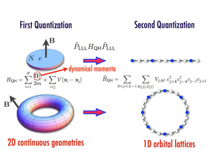
Figure 1: Pictorial representation of the effective dimensional reduction realized when going from the first to the second quantization representation of the QH Hamiltonian.

In the sums defining the Hamiltonian (2) we leave implicit the constraint that orbital indices $j\pm k$ and $j\pm l$ are integer. This implies that these sums go over both triples $(j,k,l)$ with all entries integer and triples $(j,k,l)$ with all entries half-odd integer. With $j$ being restricted to the interval $[0,L-1]$, $j$ thus takes on the $2L-3$ consecutive values

$$j_{\sf min}=\frac{1}{2},1,\frac{3}{2},2,\dotsc,j_{\sf m}=\frac{L-1}{2},\dotsc,j_{\sf max}=L-\frac{3}{2}.$$ (4)

The sum over $k$ in Eq. (3) starts at $k_{\sf min}=\frac{1}{2}$($1$) if $j$ is half-odd integer(integer), ends at $k_{\sf max}=\min(j,L-1-j)$, and involves

$${\cal C}(j)=\min([j+\frac{1}{2}],[L-\frac{1}{2}-j])$$ (5)

terms, with $[k]$ representing the integer part of $k$. The “middle” allowed angular momentum value is $j_{\sf m}$.

geometry	$L$  (Laughlin)	$N_{\Phi}$	$\eta_{k}(j,1)$	$\phi_{r}(z)$
disk	${\sf q}N-{\sf q}+1$	$L$	$k\,2^{-j+1}\sqrt{\frac{1}{j}{2j\choose j+k}}$	$\frac{1}{\sqrt{2\pi 2^{r}r!}}\,z^{r}e^{-\frac{1}{4}|z|^{2}}$
cylinder	${\sf q}N-{\sf q}+1$	$L$	$2(8/\pi)^{1/4}\kappa^{3/2}\,k\,e^{-\kappa^{2}k^{2}}$	$(4\pi^{3})^{-1/4}\sqrt{\kappa}\,e^{-\frac{1}{2}(x-r\kappa)^{2}+ir\kappa y}$
sphere	${\sf q}N-{\sf q}+1$	$L-1$	$k\sqrt{\frac{2N_{\Phi}-2}{j(N_{\Phi}-j)}{N_{\Phi}\choose j-k}{N_{\Phi}\choose j+k}/{2N_{\Phi}\choose 2j}}$	$\sqrt{\frac{N_{\Phi}+1}{4\pi}{N_{\Phi}\choose r}}[e^{-i\frac{\varphi}{2}}\sin(\frac{\theta}{2})]^{r}[e^{i\frac{\varphi}{2}}\cos(\frac{\theta}{2})]^{N_{\Phi}-r}$
torus	${\sf q}N$	$L$	$\displaystyle 2(8/\pi)^{1/4}\kappa^{3/2}\,\sum_{s\in\mathbb{Z}}(k+sL)\,e^{-\kappa^{2}(k+sL)^{2}}$	$\displaystyle\sum_{s\in\mathbb{Z}}\phi_{r+sL}^{\mbox{\scriptsize cylinder}}$

Table 2: Interactions $\eta_{k}(j,1)$ for various geometries. $L$ is the number of orbitals in incompressible QH systems for filling fractions $\nu=1/{\sf q}$, with ${\sf q}$ an odd integer. In the disk geometry $\eta_{k}(j,1)\rightarrow 2\pi^{-\frac{1}{4}}j^{-\frac{3}{4}}k\exp(-\frac{k^{2}}{2j})$ in the limit where $k\ll j$ and not necessarily $k^{2}\ll j$. The inverse radius of the cylinder or torus (in the $y$-direction) is $\kappa=2\pi/L_{y}$. $N_{\Phi}$ is the number of flux quanta threading the system. For geometries without boundaries, the relation between $N_{\Phi}$ and $L$ is unambiguous. We set $N_{\Phi}=L$ for the disk and cylinder.

The structure of Eq. (2) preserves total angular momentum $J$. The interaction Hamiltonian thus manifestly acts only on guiding center variables, while leaving the dynamical momenta (related to the Landau level index) invariant. The one dimensional sum in Eq. (2) is intimately related to the dimensional reduction that the QH system exhibits. Disparate systems that exhibit topological orders also display dimensional reductions. NO ; NOC-Holo

A broad class of rotationally invariant Hamiltonians in the LLL can be written as a sum of Haldane pseudopotentials ($\{H_{V_{m}}\}$) of order $m=1,2,\ldots$,

$$\widehat{H}_{\sf QH}=\sum_{m>0}g_{m}H_{V_{m}},$$ (6)

with general coefficients $g_{m}$. In what follows, we first discuss the lowest order pseudopotential and then detail the algebraic structure associated with it and all higher order pseudopotentials.

II.2 Lowest order Haldane pseudopotential or the Trugman-Kivelson model

It is a complex task to analytically resolve the spectral properties of $\widehat{H}_{\sf QH}$. It is well-known that Laughlin states, $|\Psi_{\nu}\rangle$, characterized by an odd integer $\sf q$ (${\sf q}\in\{1,3,5,\cdots\}$), with $\nu=1/{\sf q}$ being the filling fraction in the thermodynamic limit, are ground states of the separable lowest order Haldane pseudopotential or Trugman-Kivelson Hamiltonian Trugman ; Haldane

$$H_{V_{1}} = \sum_{0<j<L-1}\;\sum_{k(j),l(j)}\eta_{k}\eta_{l}\ c^{\dagger}_{j+k}c^{\dagger}_{j-k}c^{\;}_{j-l}c^{\;}_{j+l}\ ,$$ (7)

where the sums satisfy the same constraints as those in Eq. (2). The summation is performed over $k,l$ in accord with the convention of Eq. (3), and the coefficients $\eta_{k(l)}\equiv\eta_{k(l)}(j,1)$ depend on the geometry (see Table 2).

From the definition of the filling fraction in QH systems (see Tables 1 and 2),

$$\nu=\frac{N-1}{L-1}=\frac{N(N-1)}{2J_{\sf m}}=\frac{p}{q}\ ,$$ (8)

where $J_{\sf m}=N\,j_{\sf m}$ is the total angular momentum of the Laughlin state $|\Psi_{\nu}\rangle$ and $p,q$ are relatively prime integers.

We enforce a hard wall constraint on the disk and the cylinder that limits the available Landau level orbitals to $L$ consecutive orbitals. For the compact sphere (and torus), the LLL is naturally finite dimensional. With this, the $\nu=1/3$ Laughlin state (with $N$ electrons (see Table 2)) is the unique zero energy ground state of the positive semi-definite Hamiltonian (7) for the disk, cylinder, and spherical geometries. The completely filled Landau level $\nu=1$ fluid has a unique (ground) state, which is a simple Slater determinant, but of positive energy. For $\nu<1/3$, the Laughlin state is still a zero energy ground state of Eq. (7), but additional pseudopotential terms are required to render this ground state unique. Haldane The most general radially symmetric interaction potential can be expressed as a sum of such pseudopotentials.

On the torus, Eq. (7) must be modified to read

$$H_{V_{1}} = \sum_{0<j<L}\;\sum_{0<k,l<L/2}\eta_{k}\eta_{l}\ c^{\dagger}_{j+k}c^{\dagger}_{j-k}c^{\;}_{j-l}c^{\;}_{j+l}\,.$$ (9)

Again, all integer or all half-odd integer values $(j,k,l)$ are allowed in the sum. Moreover, the operator $c_{r}$ is identified with $c_{r+L}$ due to periodic boundary conditions. These boundary conditions are also respected by the symmetry of the $\eta_{k}$ symbols on the torus, $\eta_{k+L}=\eta_{k}$. Due to center of mass degeneracy, there are $\sf q$ degenerate $\nu=1/{\sf q}$ Laughlin states on the torus. For ${\sf q}=3$, these are the unique zero energy ground states of Eq. (9). Haldane_Rez

II.3 Separability of general pseudopotentials

For simplicity, in later sections we may often have in mind the coefficients $\eta_{k}$ that define the $V_{1}$ pseudopotential. Nevertheless, as we will now illustrate, all higher ($m>1$) order pseudopotentials are of the same factorized form in terms of $\eta$ symbols as displayed in (9).

We begin with the disk geometry, where in a first quantized language, the pseudopotentials $V_{m}$ are defined asHaldane

$$V_{m}=\sum_{{\sf i<j}}P_{m}({\sf ij})\,,$$ (10)

with $P_{m}({\sf ij})$ a projector acting on the pair of particles $({\sf ij})$ and projecting onto the subspace associated with relative angular momentum $m$. In second quantization, using the basis of single-particle angular momentum eigenstates, the most general form $V_{m}$ can have is

$$H_{V_{m}} = \sum_{0<j<L-1}H_{V_{m,j}}$$

$$= \sum_{0<j<L-1}\sum_{k(j),l(j)}M^{j}_{kl;m}\;c^{\dagger}_{j+k}c^{\dagger}_{j-k}c^{\;}_{j-l}c^{\;}_{j+l}\,,$$

where conservation of total angular momentum has been used, and $H_{V_{m,j}}$ is the operator corresponding to fixed $j$ in the second line. We note that the results of this section are valid for both fermions and bosons, where for the latter case, we must replace Eq. (3) with the more symmetric definition,

$$\sum_{k(j)}=\frac{1}{2}\sum_{0\leq|k|\leq\min(j,L-1-j)}\,,$$ (12)

and similarly for $\sum_{l(j)}$. Let us now consider the action of $H_{V_{m}}$ on states with two particles. The operator $H_{V_{m,j}}$ apparently projects any pair state with total angular momentum $2j$ onto a state with the same total angular momentum, and, as we know from the definition, relative angular momentum $m$. For two particles, however, the total and relative angular momenta fully specify the state. Therefore, $H_{V_{m,j}}$ is the projection onto the unique two-particle state specified by the quantum numbers $m$, $j$. It follows from this that $M^{j}_{kl;m}$ as a matrix in $k,l$ for fixed $j$ must have rank $1$. It is further Hermitian and real (by PT-symmetry). Its most general form is therefore given by $M^{j}_{kl;m}=\eta_{k}(j,m)\eta_{l}(j,m)=\eta_{k}\eta_{l}$, where we leave implicit the $j$ and $m$ dependence of the $\eta$-symbols. Within the two-particle subspace, the operator $H_{V_{m,j}}$ is thus the orthogonal projection onto the state

$$\sum_{k(j)}\eta_{k}\,c^{\dagger}_{j+k}c^{\dagger}_{j-k}|0\rangle\,.$$ (13)

To characterize the spectrum and the eigenstates of $H_{V_{m,j}}$ within the general $N$-particle subspace will be a main focus of this paper. The characterization of $H_{V_{m}}$ as a projection operator within the two-particle subspace, however, also implies that the normalization of the state (13) must be unity independent of $j$:

$$\sum_{k(j)}(\eta_{k})^{2}=1\quad({\sf for}\;\;2j\geq m)\,.$$ (14)

The restriction is due to the fact that for $2j<m$, $\eta_{k}\equiv 0$ as will presently become apparent. An explicit formula for $\eta_{k}$ can be obtained from Eq. (13) and the fact that the normalized first quantized two-particle wave function of relative angular momentum $m$ and total angular momentum $2j$ is

$$\frac{2^{-2j}}{2\pi\sqrt{(2j-m)!m!}}\left({z_{1}+z_{2}}\right)^{2j-m}(z_{1}-z_{2})^{m}e^{-\frac{1}{4}|z_{1}|^{2}-\frac{1}{4}|z_{2}|^{2}}\,,$$ (15)

so long as $2j\geq m$. (There exists no such state otherwise.) Expressing this in second quantization, one obtains

$$\begin{split}\eta_{k}=&(-1)^{m+j-k}\sqrt{\frac{(j-k)!(j+k)!}{{2^{2j-1}(2j-m)!m!}}}\;\times\\ &{m\choose j-k}{{}_{2}}F_{1}(-j+k,-2j+m,1-j+k+m,-1)\end{split}$$ (16a)

where ${{}_{2}}F_{1}$ is a hypergeometric function. For later purposes, it is important to note that the last equation is of the following structure

$$\eta_{k}=2^{-j+1/2}\sqrt{{2j\choose m}{2j\choose j+k}}\ p_{m,j}(k)\,,$$ (16b)

where $p_{m,j}(k)$ is a polynomial in $k$ of degree $m$ and parity $(-1)^{m}$. We will prove this in Appendix A and also give a recursive formula for the $p_{m,j}$.

We note the orthogonality of the states (15) for different $j$, $m$. Working still at fixed $j$ and making the $m$-dependence of the $\eta_{k}$ explicit for now, we have, on top of Eq. (14):

$$\sum_{k(j)}\eta_{k}(j,m)\eta_{k}(j,m^{\prime})=\delta_{m,m^{\prime}}\;\;({\sf for}\;\;2j\geq m,m^{\prime})\,.$$ (17)

This observation will directly carry over to the sphere, but not to the cylinder or torus.

For the sphere, the situation is very similar, except $P_{m}({\sf ij})$ must be defined as the projection of particles $\sf i$ and $\sf j$ onto the two-particle subspace of total angular momentum ${\sf L}^{2}={\sf\ell}({\sf\ell}+1)$ with ${\sf\ell}=N_{\Phi}-m$.Haldane The quantum number $j$ now corresponds to the $z$-component of angular momentum, where $2j$ is the total ${\sf L_{z}}$ of the pair. Again this uniquely specifies a two-particle state. The same argument as given above for the disk then implies the separable form of $H_{V_{m}}$ in second quantization. Moreover, noting that each individual particle in the LLL transforms under the spin $N_{\Phi}/2$ representation of SU(2), the coefficient $\eta_{k}$ defining the state (13) for given $j$ and $m$ is simply a Clebsch-Gordan coefficient, or, written as a 3$j$-symbol,

$$\eta_{k}=(-1)^{N_{\Phi}-2j}\sqrt{4N_{\Phi}-4m+2}\times$$

$$\begin{pmatrix}N_{\Phi}/2&N_{\Phi}/2&N_{\Phi}-m\\ N_{\Phi}/2-j+k&N_{\Phi}/2-j-k&2j-N_{\Phi}\end{pmatrix}.$$ (18a)

Again, we note for later purposes the analog of Eq. (16b) for the sphere:

$$\eta_{k}=\sqrt{{N_{\Phi}\choose j+k}{N_{\Phi}\choose j-k}}\tilde{p}_{m,j}(k)\,,$$ (18b)

where the $\tilde{p}_{m,j}(k)$ are polynomials different from the $p_{m,j}(k)$, but with the same general properties noted for the latter. The equivalence of Eqs (18) and (18b) will be explained in Appendix A, where a recursive definition of the polynomials $\tilde{p}_{m,j}(k)$ is also given.

For the cylinder, we will work in a Landau gauge where the vector potential is independent of $y$, and we impose periodic boundary conditions in $y$ with period $L_{y}$.haldanerezayi94 Two-particle wave functions are then of the form $\psi(z_{1},z_{2})=f(z_{1},z_{2})e^{-\frac{1}{2}(x_{1}^{2}+x_{2}^{2})}$, where $f(z_{1},z_{2})$ is holomorphic and periodic in $y$, i.e., $f(z_{1},z_{2})=f(z_{1}+iL_{y},z_{2})=f(z_{1},z_{2}+iL_{y})$. The pseudopotential $V_{m}$ as defined for the disk does not respect this boundary condition. One must therefore work with “periodized” versions of these pseudopotentials. For this we may view the full pseudopotential as a sum over particle pairs of the Landau level projected version of an ultra-short ranged pair potentials $V_{m}(z_{1}-z_{2})$, e.g., $V_{1}(z_{1}-z_{2})=\hat{P}_{\sf LLL}\nabla^{2}\delta(z_{1}-z_{2})\hat{P}_{\sf LLL}$,Trugman and regard the cylinder-version of this potential as $V^{\sf cyl}_{m}(z_{1}-z_{2})=\sum_{\ell}V_{m}(z_{1}-z_{2}+i\ell L_{y})$. Here $\hat{P}_{\sf LLL}$ is the projection onto the LLL. Moreover, we note that $V_{m}\psi(z_{1},z_{2})$, where $\psi$ satisfies the periodic boundary conditions defined above, is still periodic under simultaneous shifts of $z_{1}$ and $z_{2}$ by $iL_{y}$, since $V_{m}$ acts only on the relative coordinate. We may thus write $V_{m}^{\sf cyl}\psi(z_{1},z_{2})={\cal P}V_{m}\psi(z_{1},z_{2})$, where ${\cal P}f(z_{1},z_{2})=\sum_{\ell}f(z_{1}+i\ell L_{y},z_{2})$.

From these considerations, it follows that $V_{m}^{\sf cyl}$ projects onto the subspace of wave functions of the following form,

$$V_{m}^{\sf cyl}\psi(z_{1},z_{2})=$$ (19)

$$\sum_{\sf{\ell}}a(R+\frac{{\sf\ell}}{2}iL_{y})(z+i{\sf\ell}L_{y})^{m}e^{\frac{1}{8}(z+i{\sf\ell}L_{y})^{2}}e^{-\frac{1}{2}x_{1}^{2}-\frac{1}{2}x_{2}^{2}},$$

where $R=(z_{1}+z_{2})/2$, $z=z_{1}-z_{2}$, $a(R)$ is a holomorphic function satisfying the periodicity $a(R+iL_{y})=a(R)$, and the ${\sf\ell}=0$ term is just $V_{m}\psi(z_{1},z_{2})$. The first exponential is picked up by first going to the symmetric gauge, there evaluating the effect of $V_{m}$, and then transforming back to Landau gauge. It is worth noting that unlike $V_{m}\psi(z_{1},z_{2})$, $V_{m}^{\sf cyl}\psi(z_{1},z_{2})$ does not in general have an $m$th order zero as $z_{1}\rightarrow z_{2}$. On the other hand, what matters is that any $\psi(z_{1},z_{2})$ satisfying $V_{m}\psi(z_{1},z_{2})\equiv 0$ also satisfies $V_{m}^{\sf cyl}\psi(z_{1},z_{2})\equiv 0$, since the first condition is equivalent to $a(R)\equiv 0$. Moreover, the converse is also true, as one may verify by a Wick rotation in both $z_{1}$, $z_{2}$ of the holomorphic part of Eq. (19) and subsequent Poisson resummation. From this it is not difficult to show via induction in $m$ that states satisfying $V_{k}^{\sf cyl}\psi(z_{1},z_{2})\equiv 0$ for all $0\leq k\leq m$, with $k$ being odd (for bosons) or even (fermions), must have at least an $(m+2)$th order zero as $z_{1}\rightarrow z_{2}$, just as it is in the other geometries. Equation (II.3) still applies with $H_{V_{m}^{\sf cyl}}$ in place of $H_{V_{m}}$. The indices on ladder operators now refer to the momentum about the cylinder axis of the orbitals they create/annihilate, in units of $\kappa\equiv 2\pi/L_{y}$. It follows from this that $H_{V_{m,j}^{\sf cyl}}$ now projects onto states of the form (19) with $a(R)=\exp(\kappa j(z_{1}+z_{2}))$. Since this defines a one-dimensional subspace, the arguments given above for the disk and sphere still apply, and $M^{j}_{kl;m}=\eta_{k}(j,m)\eta_{l}(j,m)$. Note that straightforward “periodization” of the pseudopotential preserves the normalization (14) only in the thermodynamic limit. However, on the cylinder the $\eta_{k}$ are truly independent of $j$ due to translational invariance.

For completeness, we finally give a formula for the $\eta_{k}$ in the cylinder geometry. We begin by writing Haldane’s formula for the operator $P_{m}({\sf ij})$ in disk geometry:Haldane

$$P_{m}({\sf ij})=\frac{1}{\pi}\int\int dq_{x}dq_{y}\,L_{m}[q^{2}]e^{-\frac{q^{2}}{2}+i{\mathbf{q}}\cdot({\mathbf{\tilde{r}}}_{\sf i}-{\mathbf{\tilde{r}}}_{\sf j})}\,.$$ (20)

Here, $L_{m}$ is the $m$th Laguerre polynomial, and $\mathbf{\tilde{r}}_{\sf i}=({\tilde{x}}_{\sf i},{\tilde{y}}_{\sf i})=\hat{P}_{\sf LLL}(x_{\sf i},y_{\sf i})\hat{P}_{\sf LLL}$ is the projected position or “guiding center” of the $\sf i$th particle. According to the above discussion, we can use this expression for the cylinder after the replacement $\int dq_{y}\rightarrow\sum_{q_{y}}$ where $q_{y}$ is quantized in multiples of $\kappa=2\pi/L_{y}$. $\tilde{x}$ is quantized in the same manner, which follows from the commutation relation $[\tilde{x},\tilde{y}]=i$, together with the fact that $\tilde{y}$ acquires angular character, $\tilde{y}\equiv\tilde{y}+L_{y}$. The operator $c_{r}^{\dagger}$ creates an eigenstate of $\tilde{x}$ with eigenvalue $\kappa r$. Restricting ourselves to two particles for the moment, the operator $\exp(iq_{x}(\tilde{x}_{1}-\tilde{x}_{2}))$ is diagonal in the basis $c^{\dagger}_{r_{1}}c^{\dagger}_{r_{2}}|0\rangle$, whereas the operator $\exp(iq_{y}(\tilde{y}_{1}-\tilde{y}_{2}))$ shifts the $\tilde{x}$ eigenvalue of particle $1$ (particle $2$) by $-q_{y}$ (by $q_{y}$). These observations lead to the identification of the operator $\sum_{\pm}e^{\pm i{\mathbf{q}}\cdot({\mathbf{\tilde{r}}}_{\sf i}-{\mathbf{\tilde{r}}}_{\sf j})}$ with the second quantized operator $\sum_{\pm}\sum_{r_{1},r_{2}}e^{-iq_{x}q_{y}}e^{iq_{x}\kappa(r_{1}-r_{2})}c_{r_{2}\mp q_{y}}^{\dagger}c_{r_{1}\pm q_{y}}^{\dagger}c^{\;}_{r_{1}}c^{\;}_{r_{2}}$, where the first exponential comes from an application of the Baker-Hausdorff-Campbell identity in rearranging the exponential of non-commuting operators as a product of two exponentials. In Eq. (20), and comparing with Eq. (II.3), this yields the identification of $M^{j}_{xy;m}=\eta_{x}(j,m)\eta_{y}(j,m)=\eta_{x}\eta_{y}$ with

$$\eta_{x}\eta_{y}=\; \frac{2}{\pi}\int_{-\infty}^{\infty}dq\,L_{m}[q^{2}+(x-y)^{2}]$$ (21)

$$\hskip 14.22636pt\times\,e^{{-\frac{1}{2}(q^{2}+(x-y)^{2})+iq(x+y)}}\,,$$

where we have restricted ourselves to the case $\kappa=1$. The general case is obtained by letting $x\rightarrow\kappa x$ and similarly for $y$. One can write a compact expression for Eq. (21) in terms of Hermite polynomials of even order

$$\eta_{x}\eta_{y}=\; \frac{e^{-(x^{2}+y^{2})}}{2^{2m-3/2}\sqrt{\pi}\,m!}\sum_{l=0}^{m}(-1)^{l}\binom{m}{l}\,$$ (22)

$$\hskip 14.22636pt\times\,H_{2m-2l}[x+y]\,H_{2l}[x-y]\,,$$

by using the series expansion

$$L_{m}[q^{2}+(x-y)^{2}]=\; \frac{(-1)^{m}}{2^{2m}\,m!}\sum_{l=0}^{m}\binom{m}{l}\,$$ (23)

$$\hskip 5.69046pt\times\,H_{2m-2l}[q]\,H_{2l}[x-y]\,,$$

and performing integration over $q$. The above expression (22) readily simplifies once we transform to an $X,Y=(x\pm y)$ coordinate frame, express the Hermite polynomials in Eq. (22) via standard creation operators $a_{X,Y}^{\dagger}$ acting on Gaussians in $X,Y$, whence this reduces to $[(a_{X}^{\dagger})^{2}-(a_{Y}^{\dagger})^{2}]^{m}$ or, equivalently, $[4\tilde{a}^{\dagger}_{x}\tilde{a}^{\dagger}_{y}]^{m}$, with $\tilde{a}^{\dagger}_{x}$ scaling as $(\frac{1}{2}\partial_{x}-x)$, acting on a Gaussian in $x$ multiplied by a Gaussian in $y$. In the aftermath, the right hand side of Eq. (22) factorizes into decoupled functions in $x$ and $y$ as the left hand side implies with

$$\eta_{x}=\frac{e^{-x^{2}}}{2^{\frac{m}{2}-\frac{3}{4}}\,\sqrt{m!\sqrt{\pi}}}\ H_{m}[\sqrt{2}\,x]\,,$$ (24)

which are given in Table 3 for $m=0,\cdots,7$. Note that Eq. (24) simplifies the expression recently given in Ref. thomale, , where higher-body pseudopotentials on the cylinder were also treated.

For the torus geometry, similar arguments could be made for the separated form of the pseudopotentials. Instead, we refer to the relation between the second quantized forms of these potentials for the cylinder and torus geometries given in Section II.5.

$m$	$\eta_{x}\times(\pi/8)^{1/4}\exp[{x^{2}}]$
$0$	$1$
$1$	$2x$
$2$	$\sqrt{1/2}\,(4x^{2}-1)$
$3$	$\sqrt{2/3}\,x(4x^{2}-3)$
$4$	$\sqrt{1/24}\,(16x^{4}-24x^{2}+3)$
$5$	$\sqrt{1/30}\,x(16x^{4}-40x^{2}+15)$
$6$	$\sqrt{1/720}\,(64x^{6}-240x^{4}+180x^{2}-15)$
$7$	$\sqrt{1/1260}\,x(64x^{6}-336x^{4}+420x^{2}-105)$

Table 3: The polynomial parts of the coefficients $\eta_{x}$ defining the $m$th Haldane pseudotential in second quantization as in Eq. (7) for a cylinder with $\kappa=1$. For general cylinders, $\eta_{x}$ can be obtained from the given expressions via substitution $x\rightarrow\kappa x$ and overall multiplication by $\sqrt{\kappa}$.

II.4 Quantum Hall algebra

We are interested in identifying the algebra of interactions relevant for the QH problem. Define the operators

$$T_{js;m}^{+} = \!\!\sum_{k(j)}\eta_{k}^{2s-1}c^{\dagger}_{j+k}c^{\dagger}_{j-k}\ ,\ T_{js;m}^{-}=\!\!\sum_{k(j)}\eta_{k}^{2s-1}c^{\;}_{j-k}c^{\;}_{j+k}$$

$$T_{js;m}^{z} = \frac{1}{2}\sum_{k(j)}\eta_{k}^{2s}(n_{j+k}+n_{j-k}-1)\ ,$$ (25)

where $s\in\mathbb{Z}$, and the number operator is defined as $n_{j+k}=c^{\dagger}_{j+k}c^{\;}_{j+k}$ and, as throughout, the sum is performed over $k$ following the convention of Eq. (3). These operators close an infinite-dimensional affine Lie algebra without a central extension

$${[}T_{js;m}^{+},T_{js^{\prime};m}^{-}] = 2\,T_{j(s+s^{\prime}-1);m}^{z}$$

$${[}T_{js;m}^{z},T_{js^{\prime};m}^{\pm}] = \pm\,T_{j(s+s^{\prime});m}^{\pm}.$$ (26)

With these, the lowest order Haldane pseudopotential of Eq. (9) becomes

$$H_{V_{1}} = \sum_{0<j<L-1}T^{+}_{j1;1}T^{-}_{j1;1},$$ (27)

which explicitly displays its positive semi-definite character ($g_{1}>0$ in Eq. (6)). For this special case, it is then known that the Hamiltonian has zero energy ground states at filling fraction $\nu\leq 1/3$, as we pointed out above and will be analyzed in more detail in later sections.

Far more generally, a generic LLL QH Hamiltonian of the form of Eq. (6) can be written as

$$\widehat{H}_{\sf QH} = \sum_{m}g_{m}\sum_{0<j<L-1}T^{+}_{j1;m}T^{-}_{j1;m}.$$ (28)

Now here is an important point whose meaning will become clear in future sections: within each sector of fixed $m$ and $j$, the argument in the sum of Eq. (28) is of the form of an exactly-solvable RG pairing Hamiltonian (Eq. (54)).

II.5 Topological aspects of the Quantum Hall problem: An exact equivalence of the disk, cylinder, and spherical geometries

In the following, we will be interested in the task of characterizing zero energy states or “zero modes”. To make the discussion lucid we will concentrate on the zero modes of the $H_{V_{1}}$ pseudopotential Hamiltonian. As we will discuss in Section IV.1, the latter are constrained by the condition

$$T^{-}_{j1;1}|\Psi\rangle=0$$ (29)

for all $j$, where $T^{-}_{j1;1}$ is defined in terms of the parameters $\eta_{k}$ given in Table 2 for various geometries. Despite the different appearance of these coefficients, the tasks of finding the zero energy eigenstates (zero modes) of $V_{1}$ for the disk, cylinder, and sphere are exactly equivalent, for which we will now provide appropriate transformations in second quantization. It is intuitive that such transformations exist, as it is well appreciated that universal features of topologically ordered states are insensitive to geometric details, and only depend on the genus number (number of handles) of the system.wen Such universal features do not generically include the counting of zero modes (at filling factors below the incompressible one). However, for “fixed point” Hamiltonians such as the parent Hamiltonians of the Laughlin states, this is the case. At the first quantized level, this is a manifestation of the polynomial structure wave functions display for the disk/cylinder/sphere geometries, which has been used extensively in the derivation of counting formulas for zero modes, both for the $V_{1}$ pseudopotential as well as other parent Hamiltonians. RR ; ardonne

Note that the disk, cylinder, and sphere all have vanishing genus number (while the genus number of the torus is $1$). Below we will show how the equivalence between zero modes for these different geometries is recovered in second quantization. As evident from Table 2, the generic structure of LLL orbitals in these geometries is

$$\phi_{r}={\cal N}_{r}\ \xi^{r}\times(r{\sf-independent~{}function}),$$ (30)

where $\xi=z$, $e^{\kappa z}$, $u/v$ for the disk, cylinder, and sphere, respectively, is a holomorphic factor, with $u=e^{-i\frac{\varphi}{2}}\sin(\frac{\theta}{2})$, $v=e^{i\frac{\varphi}{2}}\cos(\frac{\theta}{2})$, and ${\cal N}_{r}$ is a geometry-dependent normalization factor. General LLL wave functions are thus polynomials in $\xi$. Note that for a cylinder with inverse radius $\kappa\rightarrow 0$, we have ${\cal N}_{r}\equiv 1$. Consider now the similarity transformation that acts via

$$c^{\;}_{r}\rightarrow Sc^{\;}_{r}S^{-1}={\cal N}_{r}c^{\;}_{r},$$ (31)

where ${\cal N}_{r}$ corresponds to any given geometry. We can think of this transformation as changing the normalization conventions of polynomials for the $\kappa=0$ cylinder to that of any other geometry. Specifically, we may take $S=S_{\sf c}\equiv\exp[\frac{1}{2}\kappa^{2}\sum_{r}r^{2}c_{r}^{\dagger}c^{\;}_{r}]$ for a cylinder at finite $\kappa$, $S=S_{\sf d}\equiv\exp[\frac{1}{2}\sum_{r}\ln(2^{r}r!)c^{\dagger}_{r}c^{\;}_{r}]$ for the disk, and $S=S_{\sf s}\equiv\exp[-\frac{1}{2}\sum_{r}\ln{N_{\Phi}\choose r}c^{\dagger}_{r}c^{\;}_{r}]$ for the sphere. Let us denote by $t^{+}_{j}$, $t^{-}_{j}$, $t^{z}_{j}$ the operators defined in Eq. (II.4) with $\eta_{k}\equiv k^{m=1}$ ($t^{\zeta}_{j}=t^{\zeta}_{j;m=1}$, with $\zeta=\pm,z$). Equation (29) with $T^{-}_{j1;1}=t^{-}_{j}$ then corresponds to the $\kappa=0$ cylinder. It is further easy to verify that the operators $T^{-}_{j1;1}$ for a general cylinder, a disk, or a sphere are then obtained via

$$T^{-}_{j1;1}=f_{j}St^{-}_{j}S^{-1}\,,$$ (32)

see Fig. 2, where $f_{j}$ is a positive factor that depends on the geometry and $j$, and $S$ depends on the geometry as shown above. Therefore, if $|\Psi\rangle$ satisfies $t^{-}_{j}|\Psi\rangle=0$, then $S|\Psi\rangle$ satisfies Eq. (29), i.e., $T^{-}_{j1;1}S|\Psi\rangle=0$. It is thus sufficient in principle to work in the $\kappa=0$ cylinder geometry, and study the zero modes of the operators $t^{-}_{j}$. Note that we could always obtain the coefficients $f_{j}$ from the condition (14) if desired.

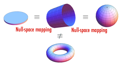
Figure 2: Topological equivalence between geometries sharing the same genus number.

We caution that for higher $m$, the one-to-one correspondence between pseudopotentials in different geometries ceases to hold in the strict sense of Eq. (32). The reason for this is that states related by the transformations defined above generally correspond to the same polynomials in the first quantized description for the respective geometries. For $m>1$, however, the rank 1 projectors $H_{V_{m,j}}$ of Eq. (II.3) will in general project onto states having a different polynomial structure for the different geometries. On the other hand, we still have the following statement: For fixed $j$, the transformed states $St^{+}_{j;m}|0\rangle$ for $0\leq m\leq{\sf M}$ (and $m$ even/odd for bosons/fermions here and below) span the same subspace as the states ${T}^{+}_{j1;m}|0\rangle$ defined in Eq. (13). Here, the ${T}^{+}_{j1;m}$ and the transformation $S$ refer to the same geometry. The reason for this is that in any geometry, the $\eta_{k}$’s are proportional to an $m$th order polynomial in $k$ with parity $(-1)^{m}$ (see Eqs. (16b), (18b), and (22)), and the $\eta_{k}$ defining $t^{+}_{j;m}$ are just equal to $k^{m}$. All other $k$-dependent factors are independent of $m$ and are taken care of by the transformation $S$. Within the two-particle sub-space, the common null space of the operators $H_{V_{m,j}}={T}^{+}_{j1;m}{T}^{-}_{j1;m}$, $0\leq m\leq{\sf M}$, is just the space orthogonal to all the states ${T}^{+}_{j1;m}|0\rangle$, and similarly the common null space of the “transformed” operators $(St^{-}_{j;m}S^{-1})^{\dagger}St^{-}_{j;m}S^{-1}$, $0\leq m\leq{\sf M}$ is the space orthogonal to all the states $St^{+}_{j;m}|0\rangle$, $0\leq m\leq{\sf M}$. Thus in any geometry, the operators $H_{V_{m,j}}$, for $0\leq m\leq{\sf M}$, always have the same common null space as the operators $(St^{-}_{j;m}S^{-1})^{\dagger}St^{-}_{j;m}S^{-1}$. This statement immediately carries over from the two-particle subspace to the full Fock space, since the operators in question are two-body operators. This will be of some importance in Section V.

Note that the above equivalence of null spaces holds for fixed particle number and number of Landau level orbitals. Working with a finite number of orbitals requires “hard orbital cutoffs” in the cylinder and disk geometries, but is the usual situation for the sphere. There is thus no contradiction with the common knowledge that these three geometries have different numbers of edge modes. Edge modes are present, in particular, for the usual infinite or half-infinite orbital lattice associated to the cylinder or disk geometry, respectively. Conversely, however, edge modes can be present in the spherical geometry as well, if, say, we populate only the northern half with a FQH state having an edge at the equator.

We finally observe that if $\eta_{k}^{\sf cyl}$ corresponds to the pseudopotential $V_{m}$ on the cylinder, then for the torus it can always be obtained by further periodizing the cylinder. This can be done directly in second quantization:

$$\eta_{k}^{\sf tor}=\sum_{\ell}\eta^{\sf cyl}_{k+\ell L}\,.$$ (33)

Here and in Table 2, we restrict ourselves to tori with purely imaginary modular parameter $\tau=iL_{y}/L_{x}=2\pi i/\kappa^{2}L$, where we introduced $L_{x}=\kappa L$.

III Strongly-coupled states of matter

In this section, we relate the QH Hamiltonian of Section II to the hyperbolic RG type models encountered, for instance, in the study of $(p_{x}+ip_{y})$ superconductors. In particular, in Section III.1 we demonstrate that within each sector of fixed $m$ and $j$, the Hamiltonian of Eq. (28) represents a new exactly-solvable model, that we call QH-RG, which belongs precisely to the hyperbolic RG class. We then examine (Section III.2) the Hilbert space dimension associated with the QH-RG problem. In each such sector of fixed $j$ and $m$, the spectral problem can be determined via Bethe Ansatz as we explicitly demonstrate in Section III.3. We conclude our analysis of the QH-RG Hamiltonian in this section, by highlighting the symmetry properties of the RG equations (Section III.4). The full problem formed by the sum of all (generally non-commuting) QH-RG Hamiltonians will be investigated in Section IV.

III.1 An exactly-solvable model

The XXZ Gaudin algebra NuclPhysB is an affine Lie algebra generated by operators ${\sf S}^{z}(x),{\sf S}^{\pm}(x)$ with commutation relations

$$\left[{\sf S}^{z}(x),{\sf S}^{\pm}(y)\right] = \pm\left(X(x,y){\sf S}^{\pm}(x)-Z(x,y){\sf S}^{\pm}(y)\right),$$

$$\left[{\sf S}^{+}(x),{\sf S}^{-}(y)\right] = 2X(x,y)\left({\sf S}^{z}(x)-{\sf S}^{z}(y)\right),$$ (34)

in terms of anti-symmetric functions $X(x,y)$ and $Z(x,y)$ satisfying the following condition for all $x$, $y$ and $z$

$$\left[Z(x,y)-Z(x,z)\right]X(y,z)-X(x,y)X(x,z)=0.$$ (35)

A representation of the XXZ Gaudin algebra in terms of a number ${\cal C}(j)$ (see Eq. (5)) of $su(2)$ spins, $\{S^{z}_{jk},S^{\pm}_{jk}\}$, labeled by the (in principle arbitrary) quantum numbers $j\in[j_{\sf min},j_{\sf max}]$ and $k\in[k_{\sf min},k_{\sf max}]$ is given by

$${\sf S}_{j}^{z}(x) = -\frac{1}{2}-\sum_{k(j)}Z(x,\eta_{k})S^{z}_{jk},$$

$${\sf S}_{j}^{\pm}(x) = \sum_{k(j)}X(x,\eta_{k})S^{\pm}_{jk},$$ (36)

with $\eta_{k}$ being arbitrary parameters (eventually we will equate these general parameters to be the very same constants $\eta_{k}(j,m)$ that appeared in our decomposition of the Haldane pseudopotentials). In this representation one can define a set of ${\cal C}(j)$ linearly independent constants of motion, which commute among themselves

$$R_{jk} = S^{z}_{jk}-\sum_{l(j),l\neq k}X(\eta_{k},\eta_{l})\left(S^{+}_{jk}S^{-}_{jl}+S^{-}_{jk}S^{+}_{jl}\right)$$ (37)

$$- 2\sum_{l(j),l\neq k}Z(\eta_{k},\eta_{l})S^{z}_{jk}S^{z}_{jl},$$

Linear combinations of these operators allow for the construction of an exactly solvable RG Hamiltonian

$$H_{{\sf G}j} =\sum_{k(j)}\epsilon_{k}S^{z}_{jk}$$ (38)

$$-\sum_{k(j),l(j)}(\epsilon_{k}-\epsilon_{l})X(\eta_{k},\eta_{l})S^{+}_{jk}S^{-}_{jl}$$

$$-\sum_{k(j),l(j)}(\epsilon_{k}-\epsilon_{l})Z(\eta_{k},\eta_{l})S^{z}_{jk}S^{z}_{jl}.$$

The eventual $m$ and $j$ dependence of $H_{{\sf G}j}$ stems from that of the generators in Eq. (III.1). This generic RG Hamiltonian commutes with the squared spin operators ${\bf S}_{jk}^{2}=S^{z}_{jk}(S^{z}_{jk}-1)+S^{+}_{jk}S^{-}_{jk}$, and with the total spin operator ${\bf S}_{j}=\sum_{k(j)}{\bf S}_{jk}$.

A consequence of the Jacobi identity, Eq. (35), is that

$$X(x,y)^{2}-Z(x,y)^{2}=\Gamma,$$ (39)

where $\Gamma$ is a constant independent of $x$ and $y$. In this work we will focus on the properties of the hyperbolic RG model, which correspond to $\Gamma=-\bar{g}^{2}/4<0$. It is interesting to mention that the $p_{x}+ip_{y}$ integrable pairing model belongs to this class. Romb Any set of functions $X(x,y)$ and $Z(x,y)$ that fulfills Eqs. (35) and (39), can be mapped onto the following parameterization NuclPhysB

$$X(x,y)=-\bar{g}\frac{xy}{x^{2}-y^{2}},\ \ \ Z(x,y)=-\frac{\bar{g}}{2}\frac{x^{2}+y^{2}}{x^{2}-y^{2}}.$$ (40)

Using this parameterization, setting $\epsilon_{k}=\lambda_{j}\eta^{2}_{k}$, and subtracting a diagonal term $-\bar{g}\sum_{k(j)}\eta^{2}_{k}{\bf S}^{2}_{jk}$, one obtains an interesting form for the Hamiltonian of Eq. (38)

$$H_{{\sf G}j} = \lambda_{j}(1+\bar{g}(S_{j}^{z}-1))\sum_{k(j)}\eta_{k}^{2}S^{z}_{jk}$$ (41)

$$+\lambda_{j}\bar{g}\sum_{k(j),l(j)}\eta_{k}\eta_{l}S^{+}_{jk}S^{-}_{jl},$$

where for a fixed $j$, $j\pm k,j\pm l$ are all non-negative integers in the interval $[0,L-1]$ as before. The parameters $\lambda_{j},\bar{g}$ (which can be positive or negative) and $\eta_{k}$ are arbitrary in principle.

A possible fermionic representation of the $su(2)$ spin algebra, similar to the $p_{x}+ip_{y}$ superconductor Romb is given by

$$S_{jk}^{+} = c^{\dagger}_{j+k}c^{\dagger}_{j-k}\ ,\ S_{jk}^{-}=c^{\;}_{j-k}c^{\;}_{j+k}$$

$$S_{jk}^{z} = \frac{1}{2}(n_{j+k}+n_{j-k}-1).$$ (42)

As mentioned above, the value of $j$ is arbitrary in the interval $[\frac{1}{2},L-\frac{3}{2}]$ (see Eq. (4)). However, once the value of $j$ is chosen, it classifies completely the basis states into an active space of ${\cal C}(j)$ active levels ${\bf k}\equiv[j+k,j-k]$, and a set of inactive levels $\{i_{1},i_{2},\cdots,i_{L-2{\cal C}(j)}\}$ which includes the remaining $L-2{\cal C}(j)$ levels left out of the active set. This classification allows us to define an $su(2)$ vacuum state $|\nu(j)\rangle$, which is annihilated by the lowering operators $S_{jk}^{-}|\nu(j)\rangle=0$ as

$$|\nu(j)\rangle\equiv|\{\nu_{jk}\}\rangle\otimes|\nu_{\sf in}\rangle.$$ (43)

The seniorities $\nu_{jk}$ are defined as follows: $\nu_{jk}=0$ if the level ${\bf k}$ is empty or doubly occupied (not in the vacuum $|\{\nu_{jk}\}\rangle$), and $\nu_{jk}=\pm 1$ if there is a single electron with momentum $j\pm k$ (see Fig. 3). The two different non-zero values for the seniorities $\nu_{jk}$ are associated with a spin 1/2 degree of freedom.

The state $|\nu_{\sf in}\rangle$ defines a configuration of $N_{\sf in}$ electrons distributed among the $L-2{\cal C}(j)$ inactive levels

$$|\nu_{\sf in}\rangle\equiv c^{\dagger}_{i_{1}}c^{\dagger}_{i_{2}}\cdots\,c^{\dagger}_{i_{N_{\sf in}}}\ |0\rangle.$$ (44)

Therefore, the vacuum is an eigenstate of the associated operator $S_{jk}^{z}$

$$S_{jk}^{z}|\nu(j)\rangle=\frac{1}{2}(|\nu_{jk}|-1)|\nu(j)\rangle\equiv-s_{jk}|\nu(j)\rangle.$$ (45)

Additional symmetries become manifest in the fermionic language. In particular, the $su(2)$ algebra

$$\tau_{jk}^{+} = c^{\dagger}_{j+k}c^{\;}_{j-k}\ ,\ \tau_{jk}^{-}=c^{\dagger}_{j-k}c^{\;}_{j+k}$$

$$\tau_{jk}^{z} = \frac{1}{2}(n_{j+k}-n_{j-k}),$$ (46)

generates the gauge symmetry of $H_{{\sf G}j}$ responsible for Pauli blocking, NuclPhysB with seniority $\nu(j)$ representing a good quantum number. This gauge symmetry is no longer a symmetry of pseudopotential Hamiltonians $H_{V_{m}}$ formed by the sum of the individual Hamiltonians $H_{{\sf G}j}$ for each value of $j$. Similarly, the total angular momentum operator defined as ($r$ is an integer)

$$\hat{J}=\sum_{r=0}^{L-1}r\ n_{r},$$ (47)

is also a symmetry of the Hamiltonian $H_{{\sf G}j}$. It is easy to check that $[\hat{J},S_{jk}^{\pm}]=\pm 2jS_{jk}^{\pm}$, implying that the angular momentum of each pair is $2j$ and that the maximum possible angular momentum of each electron in the pair is also $2j$. Moreover, the state $j$ does not participate in pairing, and it can be empty or occupied by a single electron, defining a seniority $\nu_{j0}=0,1$, respectively.

Assume that the total number of electrons, a good quantum number, is $N=2M+N_{\nu(j)}$, where $M$ is the number of pairs with angular momentum $2j$, and $N_{\nu(j)}=N_{\sf b}+N_{\sf in}$ is the total number of unpaired electrons with

$$N_{\sf b}=\sum_{k(j)}|\nu_{jk}|=\sum_{k(j)}(1-2s_{jk}).$$ (48)

Note that the total number of electrons has three contributions: (i) the $2M$ electrons that participate in the pair mechanism, and the unpaired electrons $N_{\nu(j)}$ which in turn are split into (ii) $N_{\sf b}$ electrons blocking active levels (see the two $\nu_{jk}=\pm 1$ cases shown in Fig. 3) and (iii) $N_{\sf in}$ electrons distributed among inactive levels. Then a seniority configuration of $N_{\nu(j)}$ unpaired electrons

$$[j+k_{1},j+k_{2},\cdots,j+k_{N_{\sf b}};{{i_{1}},{i_{2}},\cdots,{i_{N_{\sf in}}}}],$$ (49)

is an eigenstate of $H_{{\sf G}j}$ with $M$ pairs, $|\Phi_{M\nu(j)}\rangle$, satisfies

$$S^{z}_{j}|\Phi_{M\nu(j)}\rangle = \frac{1}{2}\left(2M+N_{\nu(j)}-{\cal C}(j)\right)|\Phi_{M\nu(j)}\rangle$$ (50)

$$= (M-\sum_{k(j)}s_{jk})\,|\Phi_{M\nu(j)}\rangle,$$

and has a total angular momentum $\hat{J}|\Phi_{M\nu(j)}\rangle=J|\Phi_{M\nu(j)}\rangle$

$$J = 2Mj+J_{\nu(j)},$$ (51)

where the contribution from unpaired electrons is given by

$$J_{\nu(j)}=\sum_{k(j)}|\nu_{jk}|(j+\nu_{jk}\,k)+J_{\sf in},\mbox{ with }J_{\sf in}=\sum_{j=1}^{N_{\sf in}}i_{j}.$$ (52)

Thus, one can classify the eigenstates of $H_{{\sf G}j}$ according to their total angular momentum $\hat{J}$ and $S^{z}_{j}$.

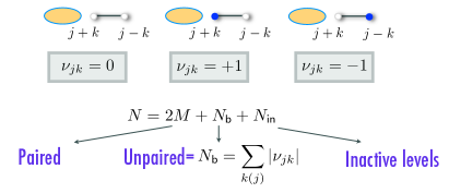
Figure 3: Possible electronic configurations for active level ${\bf k}\equiv[j+k,j-k]$, and corresponding values of their seniority $\nu_{jk}$. Dark circles correspond to an occupied orbital in $|\{\nu_{jk}\}\rangle$, while white ones to unoccupied ones. Ellipsis correspond to pairs in active levels (i.e., in ${\sf S}_{j}^{+}$). Notice that configurations with $\nu_{jk}=\pm 1$ Pauli block the corresponding level ${\bf k}$ in ${\sf S}_{j}^{+}$. Thus, active levels form either pairs or are unpaired.

The analysis above allows us to label eigenstates according to a filling fraction $\nu$ (related to $S^{z}_{j}$) and the angular momentum $J$. The filling fraction in the RG problem is, by analogy to a QH system on a disk (Eq. (8)), defined as follows:

$$\nu=\frac{N-1}{L-1}=\frac{p}{q}\leq 1,$$ (53)

with $p$ and $q$ relative prime numbers. For fixed $\nu$, the latter relation constrains allowed values of $N$ to be separated by integer multiples of $p$ since $L$ is given by the integer $L=\frac{q}{p}(N-1)+1$.

The model Hamiltonian of Eq. (41) is exactly solvable, Romb ; Ibanez meaning that its full spectrum can be determined with algebraic complexity. In the present paper, because of its relevance to QH physics, we are interested in a particular singular limit of that model. We will consider the case where $\bar{g}=-2/(2M+N_{\nu(j)}-{\cal C}(j)-2)$, leading to a term in the strongly-coupled Hamiltonian of Eq. (28), Pan

$$H_{{\sf G}j;m} =g\sum_{k(j),l(j)}\eta_{k}\eta_{l}\,c^{\dagger}_{j+k}c^{\dagger}_{j-k}c^{\;}_{j-l}c^{\;}_{j+l}$$ (54)

$$=g\ T_{j1;m}^{+}T_{j1;m}^{-},$$

with $g=\lambda_{j}\overline{g}$. In each sector of fixed pair angular momentum $2j$ and for each pseudopotential index $m$, the LLL QH Hamiltonian is identical to the QH-RG Hamiltonian of Eq. (54). We will return to the investigation of the full QH problem formed by sums of individual QH-RG Hamiltonians (see Eq. (28) in Section II.4). For the time being, we remark that the individual QH-RG Hamiltonians corresponding to different values of $j$ generally do not commute with one another; there are only four QH-RG Hamiltonians $H_{{\sf G}j}$ which are special in that they are diagonal; these correspond to $j=\frac{1}{2},1,j_{\sf max}-\frac{1}{2},j_{\sf max}$ with $j_{\sf max}$ denoting the maximal possible value of $j$ (see Eq. (4)).

It is notable that contrary to more standard pairing problems, especially those in which pairing may arise in mean-field treatments, when a Haldane pseudopotential is used, the Hamiltonian of Eq. (28) is repulsive i.e., $g>0$. Nonetheless, as we elaborate on below, in the decomposition into exactly solvable QH-RG Hamiltonians, we will find that each repulsive term associated with a given $j$ (and $m$) in Eq. (28), pairing is induced in the sense that pair fluctuations dominate correlations among electrons.

III.2 Hilbert space analysis

Given $N$ spinless fermions and $L$ orbitals, the dimension of the Hilbert state space ${\cal H}_{L}(N)$ is

$$\dim{\cal H}_{L}(N)=\binom{L}{N}=\frac{L!}{N!(L-N)!}.$$ (55)

The set of allowed total angular momenta $J$ is given by

$${\cal J}_{L}(N) = \Big{\{}\frac{N(N-1)}{2},\frac{N(N-1)}{2}+1,$$ (56)

$$\frac{N(N-1)}{2}+2,\cdots,N\left(L-\frac{(N+1)}{2}\right)\Big{\}},$$

such that

$$\dim{\cal H}_{L}(N)=\sum_{J\in{\cal J}_{L}(N)}\dim{\cal H}_{L}(N,J),$$ (57)

where ${\cal H}_{L}(N,J)$ is the Hilbert subspace with fixed total angular momentum $J$.

Given a fixed number of electrons $N$, of orbitals $L$, and angular momentum $J$, one can determine the dimension of the Hilbert space ${\cal H}_{L}(N,J)$ as follows: The dimension of ${\cal H}_{L}(N,J)$ is equal to the total number, $N_{\{m_{i}\}}$, of distinct partitions $\{m_{i}\}$=$\{m_{1},m_{2},\cdots,m_{N}\}$, $\sum_{i=1}^{N}m_{i}=J$, of the integer $J$, and can be determined with the help of the following generating function

$${\cal{Z}}(x,z)=\prod_{r=0}^{m_{\sf max}}(1+zx^{r})=\sum_{\bar{J}=0}^{\bar{m}_{\sf max}}\sum_{\bar{N}=0}^{m_{\sf max}+1}{\cal P}(\bar{N},\bar{J})\,z^{\bar{N}}x^{\bar{J}},$$ (58)

where $m_{\sf max}=L-1$ is the largest integer that may appear in the partition $\{m_{i}\}$, and $\bar{m}_{\sf max}=m_{\sf max}(m_{\sf max}+1)/2=(L-1)L/2$. The dimension of ${\cal H}_{L}(N,J)$ is

$$\dim{\cal H}_{L}(N,J)=N_{\{m_{i}\}}={\cal P}(N,J).$$ (59)

The number of partitions associated with the filling fraction of $\nu=1$, see Eq. (8), constitutes a limiting non-vanishing value, ${\cal P}(N,N(N-1)/2)=1$. [This single possible partition corresponds to the arithmetic series, $\sum_{r=0}^{N-1}r=N(N-1)/2$.]

We note that Eq. (58) corresponds to the grand canonical partition function of a system of free spinless fermions with equally spaced single particle energy levels similar to a harmonic oscillator system, and trivially constrained by a cutoff $m_{\sf max}$. That is, in Eq. (58), $z$ may be regarded as the fugacity ($e^{\beta\mu}$ with $\mu$ the chemical potential) of these particles and $x$ as the Boltzmann factor associated with the equally spaced levels ($x=e^{-\beta\varepsilon}$ with a linear energy dispersion $\varepsilon_{r}=r\varepsilon$, and inverse temperature $\beta$). Such equally spaced levels are formally similar to those of the original Landau level problem of non-interacting spinless fermions in a magnetic field (yet now sans a degeneracy of the single particle states). In our case, unlike that of standard non-interacting fermion problems, the equally spaced levels may only be occupied up to a threshold value, i.e., up to $r=m_{\sf max}$. This cutoff constraint is trivial and does not affect the Fermi function occupancy of levels which we will shortly discuss below (formally, such a cutoff may also be implemented by setting the energies of all non-allowed levels to be positive and infinite for which the corresponding Fermi function trivially vanishes as it must).

In the canonical ensemble one has to place $N$ fermions,

$$N=\sum_{r=0}^{m_{\sf max}}n_{r}$$ (60)

over $(2j+1)=m_{\sf max}+1$ levels such that the total “energy”

$$J=\sum_{r=0}^{m_{\sf max}}\varepsilon_{r}\ n_{r}$$ (61)

is fixed, with occupancies $n_{r}=0,1$. The total number of states is given by

$${\cal P}(N,J)=e^{\sf S},$$ (62)

where the entropy ${\sf S}$ is defined by the corresponding entropy of the Fermi-Dirac gas with a linear energy dispersion, and in units such that $k_{B}=1$.

It is clear that the number of partitions increases exponentially for large system sizes. A quantitative approximation for this increase can be obtained in the grand canonical ensemble in the relevant thermodynamic limit. Let us start defining the average number of particles

$$\bar{N}=z\frac{\partial\ln{\cal Z}}{\partial z}=\sum_{r=0}^{m_{\sf max}}\langle n_{r}\rangle,$$

$$\mbox{ with }\langle n_{r}\rangle\equiv\langle n_{\varepsilon}\rangle=\frac{1}{1+e^{\beta(\varepsilon-\mu)}}$$ (63)

representing the mean occupation number, and average “energy”

$$\bar{J}=-\frac{\partial\ln{\cal Z}}{\partial\beta}=\sum_{r=0}^{m_{\sf max}}\varepsilon_{r}\ \langle n_{r}\rangle,$$ (64)

The equally spaced levels $\varepsilon_{r}=r\epsilon$ imply a constant density of states (of size unity) in approximating the discrete sums in Eqs. (63) and (64) by integrals from which it is seen that average number of particles $\bar{N}$ and average “energy” are moments of the Fermi function $\langle n_{\epsilon}\rangle$.

$$\bar{N} \approx \int_{0}^{m_{\sf max}}d\varepsilon\ \langle n_{\varepsilon}\rangle\ ,\ \bar{J}\approx\int_{0}^{m_{\sf max}}d\varepsilon\ \varepsilon\,\langle n_{\varepsilon}\rangle.$$ (65)

Further corrections to the integral approximations above to the original sums over discrete states may be obtained via the Euler-Maclaurin formula.

In Eq. (65), $\mu$ and $\beta$ are Lagrange multipliers that fix the averages in Eqs. (60) and (61). The integrals of Eqs. (65) are readily evaluated,

$$\bar{N} \approx m_{\sf max}+\frac{1}{\beta}\ln\Big{(}\frac{1+e^{-\beta\mu}}{1+e^{\beta(m_{\sf max}-\mu)}}\Big{)},$$

$$\bar{J} \approx \frac{1}{2\beta^{2}}\Big{[}\beta^{2}m_{\sf max}^{2}-2\beta m_{\sf max}\ln(1+e^{\beta(m_{\sf max}-\mu)}))$$ (66)

$$- 2\,{\sf Li}_{2}(-e^{\beta(m_{\sf max}-\mu)})+2\,{\sf Li}_{2}(-e^{-\beta\mu})\Big{]},$$

where ${\sf Li}_{2}(z)=\sum_{a=1}^{\infty}\frac{z^{a}}{a^{2}}$ is the polylogarithmic function of order two. Specializing to an incompressible Laughlin fluid, if we set $N=\bar{N}$ and $m_{\sf max}=\frac{q}{p}(\bar{N}-1)$, we find, in this thermodynamic limit (whence we approximate $(\bar{N}-1)\sim\bar{N}$)) that, from the first of Eqs. (66),

$$e^{\beta\mu}\approx\frac{1-e^{\beta\bar{N}}}{e^{(1-\frac{q}{p})\beta\bar{N}}-1}.$$ (67)

Formally, for the particular case of $\frac{q}{p}=2$, Eq. (67) further simplifies to $\mu=\bar{N}$. Given also $\bar{J}$, the combination of Eq. (67) and the second of Eqs. (66) provides both $\beta$ and $\mu$.

The entropy of the free Fermi system is the sum of the entropies associated with that of the decoupled levels $\varepsilon$ (for which the probabilities of the two possible states (i.e., of having the state of energy $\varepsilon$ being occupied or empty) are $\langle n_{\varepsilon}\rangle$ and $(1-\langle n_{\varepsilon}\rangle)$ respectively) and is thus given (in the continuum integral approximation to the original discrete $\varepsilon$ sums) by

$${\sf S}=-{{\sf Tr}}\rho\ln\rho\approx-\int_{0}^{m_{\sf max}}d\varepsilon\Big{[}\langle n_{\varepsilon}\rangle\ln\langle n_{\varepsilon}\rangle$$

$$+(1-\langle n_{\varepsilon}\rangle)\ln(1-\langle n_{\varepsilon}\rangle)\Big{]},$$ (68)

where $\rho$ is the density matrix. Armed with the entropy of Eq. (68), we may next invoke Eq. (62) to compute the number of states (i.e., Hilbert space dimension). It is readily seen that the entropy is extensive in $m_{\sf max}$ and thus the system size $N$. Unfortunately, an illuminating closed form expression is not attainable.

III.3 Eigenspectrum

The model Hamiltonian $H_{{\sf G}j}$ of Eq. (54) is exactly solvable, meaning that one can write down its full eigenspectrum with algebraic complexity. The (unnormalized) eigenvectors of $H_{{\sf G}j}$ are the states

$$|\Phi_{M\nu(j)}\rangle=\prod_{\alpha=1}^{M}{\sf S}^{+}_{j}(E_{\alpha})|\nu(j)\rangle,$$ (69)

with

$${\sf S}^{+}_{j}(E_{\alpha})=\sum_{k(j)}\frac{\eta_{k}}{\eta_{k}^{2}-E_{\alpha}}\ c^{\dagger}_{j+k}c^{\dagger}_{j-k},$$ (70)

and where the seniority eigenstates $|\nu(j)\rangle$ satisfy the relation $H_{{\sf G}j}|\nu(j)\rangle=0$. Note that the structure of these equations is the same for different pseudopotential indices $m$, and only depends on the general factorized form of the Hamiltonian. To avoid cumbersome notation, as we have done in last sections, we will often omit the pseudopotential rank index $m$.

The eigenvalue equation can then be written as

$$H_{{\sf G}j}|\Phi_{M\nu(j)}\rangle = [H_{{\sf G}j},\prod_{\alpha=1}^{M}{\sf S}^{+}_{j}(E_{\alpha})]|\nu(j)\rangle$$ (71)

$$= {\cal E}_{M\nu(j)}|\Phi_{M\nu(j)}\rangle,$$

with the commutator

$$[H_{{\sf G}j},\prod_{\alpha=1}^{M}{\sf S}^{+}_{j}(E_{\alpha})] =$$

$$-2g\sum_{\alpha=1}^{M}\mathbb{S}^{+}_{j\alpha}\ \Big{(}\sum_{k(j)}\frac{\eta^{2}_{k}}{\eta^{2}_{k}-E_{\alpha}}S^{z}_{jk}+\sum_{\beta(\neq\alpha)=1}^{M}\frac{E_{\beta}}{E_{\beta}-E_{\alpha}}\ \Big{)}$$

and

$$\mathbb{S}^{+}_{j\alpha}=\left(\prod_{\gamma(\neq\alpha)=1}^{M}{\sf S}^{+}_{j}(E_{\gamma})\right)\ T^{+}_{j1}.$$ (73)

There are two distinct types of solutions:

$\bullet$ It is clear from the commutator, Eq. (III.3), that zeroing the quantity in parentheses there are solutions with eigenvalue (see Fig. 4)

$${\cal E}_{M\nu(j)}=0,$$ (74)

corresponding to the case where all the spectral parameters $E_{\alpha}$ (also known as pairons) are finite (complex-valued, in general). The RG (Bethe) equations satisfied by those pairons are of the form,

$$\sum_{\beta(\neq\alpha)=1}^{M}\frac{E_{\beta}}{E_{\beta}-E_{\alpha}}-\sum_{k(j)}s_{jk}\ \frac{\eta^{2}_{k}}{\eta^{2}_{k}-E_{\alpha}}=0,\ \forall\alpha$$ (75)

$\alpha\in[1,M]$, which can be re-written as (when $E_{\alpha}\neq 0$)

$$\sum_{k(j)}\frac{s_{jk}}{\eta^{2}_{k}-E_{\alpha}}-\sum_{\beta(\neq\alpha)=1}^{M}\frac{1}{E_{\beta}-E_{\alpha}}-\frac{Q_{j}}{E_{\alpha}}=0,\ \forall\alpha$$ (76)

with $Q_{j}=M-1-\sum_{k(j)}s_{jk}=M-1+(N_{\sf b}-{\cal C}(j))/2$. If there is one vanishing pairon, $E_{\alpha}=0$, then the following condition needs to be satisfied

$$\sum_{k(j)}s_{jk}=M-1.$$ (77)

$\bullet$ There is another class of solutions that corresponds to having one pairon $E_{M}\rightarrow\infty$, where

$${\sf S}^{+}_{j}(E_{M})\rightarrow-\frac{1}{E_{M}}\ T^{+}_{j1},$$ (78)

with the remaining pairons ($\alpha\in[1,M-1]$) being finite-valued and satisfying the RG equations

$$1+\sum_{\beta(\neq\alpha)=1}^{M-1}\frac{E_{\beta}}{E_{\beta}-E_{\alpha}}-\sum_{k(j)}s_{jk}\ \frac{\eta^{2}_{k}}{\eta^{2}_{k}-E_{\alpha}}=0.$$ (79)

For this class of solutions the corresponding eigenvalues of $H_{{\sf G}j}$ are positive(negative) (see Fig. 4)

$${\cal E}_{M\nu(j)}=2g\left(\sum_{k(j)}s_{jk}\,\eta^{2}_{k}-\sum_{\alpha=1}^{M-1}E_{\alpha}\right),$$ (80)

which simply results from the fact that $H_{{\sf G}j}$ is a positive(negative) semi-definite operator when $g>0$ $(g<0)$.

Care has to be taken with the different seniority subspaces entering in Eqs. (75) and (80) through the eigenvalues $s{{}_{jk}}$ of the $S^{z}_{jk}$ operator, Eq. (45). The total number of unpaired electrons $N_{\nu(j)}$ should have a total angular momentum $J_{\nu(j)}=jN_{\sf b}+J_{\sf in}$, and they should not couple in pairs to angular momentum $2j$. Therefore, the seniority configuration of $N_{\sf b}$ electrons $[j+k_{1},j+k_{2},\cdots,j+k_{N_{\sf b}}]$ must fulfill the condition

$$\sum^{N_{\sf b}}_{i=1}k_{i}=0.$$ (81)

We note here that for any seniority configuration $[j+k_{1},\cdots,j+k_{2},j+k_{N_{\sf b}}]$ satisfying the condition (81) there is another seniority configuration $[j-k_{1},j-k_{2},\cdots,j-k_{N_{\sf b}}]$ blocking the same pair states ${\bf k}=[j+k,j-k]$, satisfying (81), and with same set of parameters $s_{jk}$. These two solutions have the same energy Eq. (80). Hence, any eigenvalue with one infinite pairon, $M-1$ finite pairons, and non-zero seniority is at least doubly degenerate.

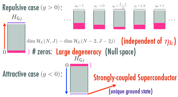
Figure 4: Eigenvalue spectrum of the repulsive and attractive QH-RG model, which is the strong-coupling limit of the hyperbolic ($p_{x}+ip_{y}$) RG model.

One can analytically determine the largest contribution to the first term in Eq. (80) for the non-zero eigenvalues

$$\sum_{k(j)}\eta^{2}_{k},$$ (82)

corresponding to $s_{jk}=1/2$, for all values of $k$. For the disk geometry, for instance, it is given by

$$\sum_{k(j)}\eta^{2}_{k}=\frac{1}{2^{2j-2}j}\sum_{k=1/2}^{j}k^{2}\binom{2j}{j+k}.$$ (83)

The sum can be easily shown to be given by

$$\sum_{k=1/2}^{j}k^{2}\binom{2j}{j+k}=j\,2^{2j-2},$$ (84)

implying that the largest contribution is

$$\sum_{k(j)}\eta^{2}_{k}=1,$$ (85)

a trivial constant value independent of $L$ and $N$. This normalization makes explicit earlier considerations which led to Eq. (14).

Inspection of Eqs. (75) or (79) tells us that the set of spectral parameters $\{E_{\alpha}\}$ is identical to the set $\{E_{\alpha}^{*}\}$, meaning that the pairons are either real-valued or if a pairon, e.g., $E_{1}$, is complex then there exists another pairon solution that is its complex conjugate, i.e., $E_{1}^{*}$. Notice that the RG equations, and consequently the spectral parameters, do not depend on the coupling strength $g$.

Therefore, all non-zero energy eigenstates are associated with spectral parameters which are all finite-valued except one, identified with $E_{M}$, which becomes infinite. Because of the latter, the total number of positive(negative) energy eigenstates is given by the number of partitions ${\cal P}(N-2,J-2j)$, which implies that the total number of zero energy eigenstates is $N_{\sf z}={\cal P}(N,J)-{\cal P}(N-2,J-2j)$. Table 4 displays some characteristic values of various dimensions for systems up to $N$=10 electrons.

$N$	$m_{\sf max}$	$J_{\sf m}$	$N_{\{m_{i}\}}$	$N_{\sf z}$	$\ell_{\frac{N}{2}}$
2	3	3	2	1	1
4	9	18	18	13	5
6	15	45	338	252	28
8	21	84	8512	6375	165
10	27	135	246448	184717	1001

Table 4: Dimension of the Hilbert space, $N_{\{m_{i}\}}$, and number of zero energy eigenstates, $N_{\sf z}$, $\ell_{M}=\binom{{\cal C}(j)}{M}-\binom{{\cal C}(j)}{M-1}$, for $\frac{q}{p}=3$ and $2j_{\sf m}=m_{\sf max}$.

The nature of the ground state of $H_{{\sf G}j}$ depends on the sign of $g$. In the repulsive ($g>0$) case, the ground state is, in general, highly degenerate and its energy is zero regardless of the system size. On the contrary, in the attractive ($g<0$) case the ground state energy is negative, non-degenerate, and grows in magnitude with system size according to Eq. (80) (see Fig. 4).

III.4 Symmetry properties of the RG equations

In this section we are interested in analyzing the consequences of having vanishing spectral parameters, i.e., a set of pairons with $E_{\alpha}=0$. This analysis unveils a symmetry relation of the RG equations that connects eigenstates with different filling fractions $\nu$.

Consider an $M$ pair state of the form ($\tilde{M}=M-N_{0}$)

$$|\Phi_{M\,\nu(j)}\rangle=({\sf S}_{j}^{+}(0))^{N_{0}}|\Phi_{\tilde{M}\nu(j)}\rangle=(T^{+}_{j0})^{N_{0}}|\Phi_{\tilde{M}\nu(j)}\rangle,$$ (86)

where we assume that $N_{0}$ pairons vanish, and $|\Phi_{\tilde{M}\nu(j)}\rangle$ is an eigenstate of $H_{{\sf G}j}$. What are the conditions necessary for $|\Phi_{M\,\nu(j)}\rangle$ to be an eigenstate of $H_{{\sf G}j}$? To address this question one needs to evaluate the commutator

$$[H_{{\sf G}j},(T^{+}_{j0})^{N_{0}}] = -g{N_{0}}(T^{+}_{j0})^{{N_{0}}-1}T^{+}_{j1}(2T^{z}_{j0}+{N_{0}}-1),$$ (87)

with $T^{z}_{j0}=S^{z}_{j}$. Since $|\Phi_{\tilde{M}\,\nu(j)}\rangle$ is also an eigenstate of $S^{z}_{j}$, the vanishing of this commutator would indicate that the states $|\Phi_{\tilde{M}\,\nu(j)}\rangle$ and $|\Phi_{M\nu(j)}\rangle$ are degenerate, i.e., share the same eigenvalue although they correspond to different filling fractions.

It follows that if the number of vanishing spectral parameters satisfies

$${N_{0}}=2(M-\sum_{k(j)}s_{jk})-1=1+2Q_{j},$$ (88)

then the states $|\Phi_{M\nu(j)}\rangle$ and $|\Phi_{\tilde{M}\,\nu(j)}\rangle$ are degenerate. Moreover, no pairons $E_{\alpha}$ converge to zero for $2(\sum_{k(j)}s_{jk}-M)+1\geq 0$. Note that the filling fractions corresponding to these two states are

$$\nu^{M}=\frac{N(N-1)}{2J}\ ,\ \nu^{\tilde{M}}=\frac{\tilde{N}(\tilde{N}-1)}{2\tilde{J}},$$ (89)

with $\tilde{N}=N-2{N_{0}}$ and $\tilde{J}=J-2{N_{0}}j$.

This symmetry relation, which is independent of the sign of the coupling $g$, has interesting and important consequences. (For a related discussion in the context of the $(p_{x}+ip_{y})$ superconductor see Ref. Romb, .) Consider the two special cases:

1. Symmetric case: In this limiting case $M=\tilde{M}$ (i.e., there are no zero-valued pairons, $N_{0}=0$)

   $$M=\frac{1+{\cal C}(j)-N_{\sf b}}{2}\Rightarrow Q_{j}=-\frac{1}{2}.$$ (90)

   For attractive interactions ($g<0$), this limiting case is associated with a non-trivial quantum critical point signaling a topological zero-temperature phase transition in the thermodynamic limit. Romb

2. Asymmetric case: ${N_{0}}=M-1$ (all but one zero-valued pairons)

   $$M={\cal C}(j)-N_{\sf b}\Rightarrow Q_{j}=\frac{M-2}{2}.$$ (91)

To get an understanding of the meaning of these particular relations, consider the case of seniority zero eigenstates, i.e., $N_{\nu(j)}=0$, $N=2M$, leading to $\nu^{M}=(2M-1)/(2j_{\sf m})$. Then, the symmetric case corresponds to $\nu^{M}=\nu^{\tilde{M}}={\cal C}(j_{\sf m})/(2j_{\sf m})(\stackrel{{\scriptstyle}}{{\rightarrow}}1/2)$, while the asymmetric case corresponds to $\nu^{M}=(2{\cal C}(j_{\sf m})-1)/(2j_{\sf m})(\rightarrow 1)$, and $\nu^{\tilde{M}}=1/(2j_{\sf m})(\rightarrow 0)$. The values displayed in parentheses correspond to the large $j$ limit, with $j$’s such that ${\cal C}(j)=[j+\frac{1}{2}]$.

IV Ground States of the full pseudopotential problem

In this section, we survey some known results pertaining to the zero energy ground states of Haldane pseudopotentials, and rigorously generalize some of these results using our second quantized formulation. In the earlier sections we analyzed the problem for fixed $m$ and $j$ RG type Hamiltonians $H_{{\sf G}j;m}$. We now turn to the full problem formed by the sum of these Hamiltonians over all $m$ and $j$ (Eq. (28)), and make use of Eq. (54) to write a generic rotationally symmetric Hamiltonian in the LLL as a sum of QH-RG Hamiltonians,

$$\widehat{H}_{\sf QH}=\sum_{m}\sum_{0<j<L-1}H_{{\sf G}j;m}.$$ (92)

As we have shown in this work, for the usual pseudopotential expansion, each term in the above sum is indeed of the RG form. In the following, we will, however, also have opportunity to consider generalizations where the $H_{{\sf G}j;m}$ are RG-terms with $\eta_{k}$’s not necessarily corresponding to a Haldane pseudopotential.

For concreteness, in what follows, we first focus on the lowest ($m=1$) pseudopotential. The structure of many of the following considerations is identical for all $m$. Generally, we will be interested in the case where the sum over $m$ in Eq. (92) is finite. The number of zero-energy states of Eq. (92) depends on how many terms with different $m$ and $j$ are included. We elaborate on this in Section IV.1. We then illustrate (Section IV.2) how notions of “inward squeezing” can be generalized to states that are defined through a Hamiltonian, rather than an analytic clustering property. In Section IV.3, we explain how the basis associated with the QH-RG Hamiltonians can be used as a new basis to expand Laughlin states. Facts concerning the conventional Slater determinant decomposition of Laughlin states are reviewed and expanded on in Section IV.4. We explicitly note a cutoff value (in particle number) beyond which some “admissible” Slater determinant states have a vanishing amplitude for the $\nu=1/3$ Laughlin state, underscore the relevance of maximally paired configurations (central to our RG approach), and further explicitly relate the squeezed state formulation, on which we present some rigorous results in Section IV.2, to “admissible” (in a Young tableau senseFrancesco ) Slater determinant states.

IV.1 Null space and frustration-free properties of $H_{V_{1}}$

From previous sections we conclude that the QH Hamiltonian can be written as a direct sum of hyperbolic QH-RG Hamiltonians

$$H_{V_{1}} = \!\!\!\sum_{0<j<L-1}H_{{\sf G}j}\ ,$$ (93)

with, in general,

$$[H_{{\sf G}j},H_{{\sf G}\bar{\jmath}}]\neq 0\ \ \ (j\neq\bar{\jmath}).$$ (94)

In this equation, we have fixed the pseudopotential index $m=1$ and simply denote $H_{{\sf G}j;m=1}=H_{{\sf G}j}$. The gauge symmetry of Eq. (46) displayed by each $H_{{\sf G}j}$ is no longer a symmetry of the QH Hamiltonian $H_{V_{1}}$, thus seniority is not conserved. Nonetheless, since Laughlin states are exact ground states, as we discussed in detail above, the Hamiltonian is still quasi-exactly solvable, at least for $\nu=1/{3}$ (and $\nu<1/3$). By this we mean that the ground state(s) can be determined exactly, and is(are) related to the integrable structure that we exposed above, but no such characterization is known for the finite energy excited states.

We are interested in understanding the properties of the null space ${\sf Ker}(H_{V_{1}})$. In the following sections, we wish to establish a series of exact analytic properties that emerge from our second quantization analysis. Let us start with the following known result, which we paraphrase as follows:Haldane ; Trugman “Given $L,N$, the Hamiltonian $H_{V_{1}}$ displays zero energy ground states $|\Psi_{\nu}^{J}\rangle$, i.e. $H_{V_{1}}|\Psi_{\nu}^{J}\rangle=0$, whenever $L\geq 3N-2$, or equivalently, $0\leq\nu=\frac{p}{q}\leq\frac{1}{3}$. The zero energy state is unique when $\nu=\frac{1}{3}$, it is in the sector $J=J_{\sf m}$, and is the Laughlin state $|\Psi^{J_{\sf m}}_{\frac{1}{3}}\rangle$”. Armed with this result, one can state a remarkable property of the null space ${\sf Ker}(H_{V_{1}})$: “$H_{V_{1}}$ is a frustration-free Hamiltonian for $0\leq\nu\leq\frac{1}{3}$”. This means that ${\sf Ker}(H_{V_{1}})$ is the common null space of all the null spaces ${\sf Ker}(H_{{\sf G}j})$.

The proof goes as follows: The states $|\Psi^{J}_{\nu}\rangle$ are zero energy ground states of $H_{V_{1}}$, which is a direct sum of positive semi-definite operators $H_{{\sf G}j}$. Therefore,

$$H_{{\sf G}j}|\Psi_{\nu}^{J}\rangle=0,\ \mbox{ for all }j,\ j_{\sf min}\leq j\leq j_{\sf max}$$ (95)

i.e., $|\Psi_{\nu}^{J}\rangle$ are zero energy ground states of each RG Hamiltonian $H_{{\sf G}j}$. Moreover, $0=\langle\Psi^{J}_{\nu}|H_{{\sf G}j}|\Psi^{J}_{\nu}\rangle=g^{2}\|T^{-}_{j1}|\Psi^{J}_{\nu}\rangle\|^{2}$ implies $T^{-}_{j1}|\Psi^{J}_{\nu}\rangle=0$ for all $j$, and filling fraction $\nu\leq 1/3$.

The results above generalize to Hamiltonians of the form $\widehat{H}_{\sf QH}=\sum_{0\leq m\leq{\sf M}}g_{m}H_{V_{m}}$, where the $g_{m}$ are positive for $(-1)^{m}=(-1)^{\sf M}$ and otherwise $0$. Then, the zero modes of this Hamiltonian are simultaneously annihilated by each operator $H_{V_{m,j}}$ defined in Section II.3. This condition is satisfiable for $\nu\leq 1/({\sf M}+2)$, and right at filling factor $\nu=1/({\sf M}+2)$ is satisfied uniquely by the Laughlin state $|\Psi_{\nu}^{J_{\sf m}}\rangle$.Haldane

We emphasize that presently, to the best of our knowledge, this frustration-free property cannot be derived from algebraic properties of the operators $H_{{\sf G}j}$ alone. Instead, the proof relies crucially on establishing the existence of ${\sf Ker}(H_{V_{1}})$ using first quantized language. It is worth noting that in going back to first quantized language, the problem is embedded in a larger Hilbert space that also contains degrees of freedom associated with dynamical momenta. It is only through an intricate interplay between guiding center degrees of freedom and dynamical momenta that the known analytical properties of Laughlin wave functions result.Haldane2011 This could hardly have been guessed from the second quantized Hamiltonian Eq. (9) alone, which describes only the guiding center variables. It is only for the right choice of orbitals $\phi_{r}(z)$, defined by the kinetic energy Hamiltonian $H_{K}$ and not by the second quantized pseudopotential Eq. (9), that the zero energy ground state of the problem can be characterized by simple analytic properties.

Note that the QH Hamiltonian differs in a crucial way from more standard frustration-free Hamiltonian studied in the literature. frustration_free In those cases the null space of the underlying local operators can be trivially characterized. It is then only the existence of a common null space, ${\sf Ker}(H)$, which is non-trivial. In the QH case, each QH-RG Hamiltonian $H_{{\sf G}j}$ is not strictly local but decays exponentially and, in addition, displays a different number of pair operators for different values of $j$. The null space of each $H_{{\sf G}j}$ can be exactly determined, but this is already a non-trivial problem since it requires a Bethe ansatz instead of a semi-simple Lie-algebraic solution.

There are four QH-RG Hamiltonians $H_{{\sf G}j}$ that are special since they are diagonal operators in the Fock basis, i.e., they commute among themselves, and correspond to $j=\frac{1}{2},1,j_{\sf max}-\frac{1}{2},j_{\sf max}$ (see Eq. (4)). Consider an expansion of a zero energy ground states of $H_{V_{1}}$, $|\Psi_{\nu}^{J}\rangle$, in a normalized Slater determinant (Fock) basis ($n_{r}=0,1$)

$$\{|\{n\}\rangle\} = \{|n_{0},n_{1},\cdots,n_{r},\cdots,n_{L-1}\rangle\}$$ (96)

$$= \Big{\{}\frac{1}{\sqrt{N!}}\prod_{r=0}^{L-1}(c^{\dagger}_{r})^{n_{r}}|0\rangle\Big{\}},$$

with $\sum_{r=0}^{L-1}n_{r}=N$, and $\sum_{r=0}^{L-1}r\,n_{r}=J$. Then, the following result follows: “All zero energy states have zero coefficients for the basis states with $(n_{0}=1,n_{1}=1)$, $(n_{0}=1,n_{2}=1)$, $(n_{L-3}=1,n_{L-1}=1)$, and $(n_{L-2}=1,n_{L-1}=1)$, in a Slater determinant expansion”. We note that this result is in agreement with the principle of “inward squeezing”. Bernevig1 ; Bernevig2

The proof of this assertion is straightforward: Assume that $|\Psi_{\nu}^{J}\rangle$ has Slater determinant basis elements with, e.g., $(n_{0}=1,n_{1}=1)$. Then, $H_{{\sf G}j=\frac{1}{2}}|\Psi_{\nu}^{J}\rangle\neq 0$, since $H_{{\sf G}j=\frac{1}{2}}=g\eta^{2}_{\frac{1}{2}}\,n_{1}n_{0}$, which contradicts the frustration-free condition of $H_{V_{1}}$. We can apply the same argument for the other three cases where the QH-RG Hamiltonians correspond to $j=1,j_{\sf max}-\frac{1}{2},j_{\sf max}$.

It turns out that the last argument can be considerably generalized and applied to a large class of Hamiltonians, as we show in the following section.

IV.2 Characterization of the “incompressible filling factor” and “inward squeezing” through the second quantized pseudopotentials

Due to the (in general) non-commutativity of the operators $H_{{\sf G}j}$, the characterization of frustration free ground states of the full Hamiltonian $\widehat{H}_{\sf QH}$ is a task that goes beyond the analysis of Section III, where the eigenstates of the individual operators $H_{{\sf G}j}$ have been systematically studied. For Haldane-pseudopotentials, the problem has been well-studied in first quantization where, e.g., for $H_{V_{1}}$, the solutions are just the $\nu=1/3$ Laughlin state and its quasi-hole excitations at $\nu<1/3$.Haldane ; Trugman There are no zero energy, hence frustration free, ground states at $\nu>1/3$. Our goal here is to understand such properties as much as possible in terms of the second quantized operators $H_{V_{m,j}}$ discussed at length in previous sections. From their second quantized form, it might not seem obvious that these operators have any common zero energy states at all for some appropriate range of $m$ and $j$, and for given $\nu$ and arbitrary system size. Here we primarily want to understand within second quantized language why, for instance, for the $V_{1}$ pseudopotential, the “incompressible” filling factor $\nu=1/3$ is special. By “special”, we allude to the fact that there can be no common zero energy state for the operators $H_{{\sf G}j;m=1}$ at filling factor $>1/3$. The analogous question can be asked for the parent Hamiltonian of the $\nu=1/{\sf q}$ Laughlin state. We emphasize, however, that our results in this section will establish rigorous bounds for the (non)existence of zero modes for a large class of Hamiltonians. The second-quantized Haldane pseudopotentials are merely special cases that satisfy these bounds. The same is true for the solvable Hamiltonians of Ref. Nakamura, .

Moreover, the questions asked here will naturally lead us to rigorously prove a squeezing principlehaldanerezayi94 ; Bernevig1 ; Bernevig2 for the zero modes of a general class of model Hamiltonians. We begin with some general notions related to squeezing. The reader unfamiliar with this concept will find a more detailed review in Section IV.4. We expand a given state $|\psi\rangle$ into occupancy eigenstates

$$|\psi\rangle=\sum_{\{n\}}C_{\{n\}}|\{n\}\rangle\,.$$ (97)

where $|\{n\}\rangle$ denotes an occupation number eigenstate $|n_{0},\dotsc,n_{L-1}\rangle$ as in Eq. (96). We call a state $|\{n\}\rangle$ with $C_{\{n\}}\neq 0$ $\psi$-expandable if there is a state $|\{n^{\prime}\}\rangle$ with $C_{\{n^{\prime}\}}\neq 0$ such that $|\{n\}\rangle$ and $|\{n^{\prime}\}\rangle$ are related as follows:

$$|\{n^{\prime}\}\rangle = |n_{0},\dotsc,n_{j_{1}-k}+1,\dotsc,n_{j_{1}}-1,\dotsc,n_{j_{2}}-1,$$ (98)

$$\hskip 14.22636pt\dotsc,n_{j_{2}+k}+1,\dotsc,n_{L-1}\rangle,$$

where $j_{1}\leq j_{2}$, and $k>0$. That is,

$$\langle\{n^{\prime}\}|c^{\dagger}_{j_{1}-k}c_{j_{2}+k}^{\dagger}c^{\;}_{j_{2}}c^{\;}_{j_{1}}|\{n\}\rangle\neq 0.$$ (99)

We will call a state $|\{n\}\rangle$ with $C_{\{n\}}\neq 0$ non-$\psi$-expandable or just non-expandable if $|\{n\}\rangle$ is not $\psi$-expandable. Further, we will say that $|\{n\}\rangle$ satisfies the generalized $r$-Pauli principle if there is no more than one particle in any $r$-consecutive orbitals.

Next we define the general class of operators to which our results will apply. We focus on fermions for simplicity, but it should be clear that analogous results can be obtained for bosons.

Consider the operators $T_{j1;m}^{-}=\sum_{k(j)}\eta_{k}(j,m)c_{j-k}c_{j+k}$ as in Eq. (II.4), where $1\leq m\leq{\sf M}$ and we have restored the dependence on $j$ and $m$ on the right hand side, subject to the constraint that $m$ and $\sf M$ are both odd. We will say that the family of operators $T_{j1;m}^{-}$ has “the independence property” if for any $j$ and for $\ell=\min(({\sf M}+1)/2,[j+\frac{1}{2}],[L-\frac{1}{2}-j])$, the $m$ distinct $\ell$-tuples $(\eta_{1}(j,m),\dotsc,\eta_{\ell}(j,m))$ have a linear span of dimension $\ell$ if $j$ is integer, and similarly the $m$ $\ell$-tuples $(\eta_{1/2}(j,m),\dotsc,\eta_{\ell-1/2}(j,m))$ if $j$ is half odd-integer.

It is easy to see that in particular, the $T_{j1;m}^{-}$ of the Haldane-pseudopotentials $H_{V_{m}}$ have the independence property for any $\sf M$, simply by appealing to the polynomial structure of the corresponding coefficients $\eta_{k}(j,m)$ identified in Section II.3.

Our results are expressed by the following theorem and simple corollaries:

Theorem: Let the operators $T_{j1;m}^{-}$, $m=1,3,\dotsc,{\sf M}$ satisfy the independence property, and let $|\psi\rangle$ be annihilated by all $T_{j1;m}^{-}$, $m=1,3,\dotsc,{\sf M}$, $j=1/2,\dotsc,L-3/2$. Then any non-expandable basis state $|\{n\}\rangle$ in the expansion of $|\psi\rangle$ satisfies the ${\sf M}+2$-Pauli principle.

Proof: For simplicity, we first consider the case ${\sf M}$=1. Note that the independence property then reduces to $\eta_{1}(j,m=1)\!\neq\!0$ ($\eta_{\frac{1}{2}}(j,m=1)\!\neq\!0$) for $j$ integer (half odd-integer).

We will prove the statement by contradiction. Suppose $|\{n\}\rangle$ is non-expandable and does not satisfy the $3$-Pauli principle. Then $\{n\}$ contains a string $11$ or a string $101$. Consider the former case. Then we have $|\{n\}\rangle=c^{\dagger}_{j+\frac{1}{2}}c^{\dagger}_{j-\frac{1}{2}}|\{\tilde{n}\}\rangle$ for some $j$, where $|\{\tilde{n}\}\rangle$ has two particles less than $|\{n\}\rangle$, and $\tilde{n}_{j\pm\frac{1}{2}}=0$. Further, for $k>\frac{1}{2}$, all states $c^{\dagger}_{j+k}c^{\dagger}_{j-k}|\{\tilde{n}\}\rangle$ have zero coefficient in $|\psi\rangle$, or else $|\{n\}\rangle$ would be $\psi$-expandable. We thus have $\langle\{\tilde{n}\}|T_{j1;1}^{-}|\psi\rangle=\eta_{\frac{1}{2}}(j,1)C_{\{n\}}\neq 0$. This contradicts $T_{j1;1}^{-}|\psi\rangle=0$. Ruling out strings $101$ works just the same.

To generalize to the case of arbitrary odd $\sf M$, we have to rule out strings of the form $10^{s}1$, with $0^{s}$ representing a string of $s$ zeros, where $s=0,\dotsc,{\sf M}$. For given $j$, form the new linear combination of operators $\widetilde{T}_{j1}^{-}=\sum_{m}a_{m}T_{j1;m}^{-}=\sum_{k(j)}\tilde{\eta}_{k}c_{j-k}c_{j+k}$, which still satisfies $\widetilde{T}_{j1}^{-}|\psi\rangle=0$. Consider integer $j$ and odd $s$. The independence property is then exactly what guarantees that we can always choose the $a_{m}$ such that $\tilde{\eta}_{k}=0$ for $k=1,\dots,(s-1)/2$ and $\tilde{\eta}_{(s+1)/2}=1$. Similarly for half-odd-integer $j$ and even $s$, where we can choose $\tilde{\eta}_{k}=0$ for $k=1/2,\dots,(s-1)/2$ and $\tilde{\eta}_{(s+1)/2}=1$. The operators $\widetilde{T}_{j1}^{-}$ thus have a “hollow core”, and allow one to contradict the assumption that a non-expandable $|\{n\}\rangle$ has the pattern $10^{s}1$ just as we did in the case ${\sf M}=1$ above. This concludes the proof of the Theorem.

For a general state $|\psi\rangle$, we now define its filling factor in an $L$-independent manner as $\nu=(N-1)/n_{\sf max}(\psi)$, where $n_{\sf max}(\psi)$ is the highest orbital index in $|\psi\rangle$ that has non-zero probability of being occupied in $|\psi\rangle$. Our main result is then the following:

Corollary 1: Let the operators $T_{j1;m}^{-}$, $m=1,3\dots,{\sf M}$ be defined as in the Theorem above. Then a state $|\psi\rangle$ annihilated by all $T_{j1;m}^{-}$ has a filling factor $\nu\leq 1/({\sf M}+2)$.

Proof: Because of the finite dimensionality of the Hilbert space, we can always find a non-$\psi$-expandable basis state $|\{n\}\rangle$. The latter satisfies the ${\sf M}+2$-Pauli principle. The densest basis state satisfying this generalized Pauli principle is clearly $10^{{\sf M}+1}10^{{\sf M}+1}1\dotsc 0^{{\sf M}+1}1$, which has filling factor equal to $1/({\sf M}+2)$. This necessitates that $|\psi\rangle$ has a filling factor less than or equal to that value.

The following Corollary establishes a notion of squeezing for any zero mode of any Hamiltonian $H=\sum_{m,j}{T^{+}_{j1;m}}T_{j1;m}^{-}$ with operators satisfying the assumptions of the Theorem. This includes Hamiltonians beyond the realm of pseudopotentials, such as those considered in Ref. Nakamura, . By “squeezing”, we mean the operations facilitated by the operators $c^{\dagger}_{j_{1}+k}c_{j_{2}-k}^{\dagger}c^{\;}_{j_{2}}c^{\;}_{j_{1}}$, $j_{1}<j_{2}$, and $k>0$, i.e., in essence the inverse of the operation defining an expandable state above. A state $|\{n\}\rangle$ can be “squeezed” from a basis state $|\{n^{\prime}\}\rangle$ if it can be obtained from $|\{n^{\prime}\}\rangle$ by repeated application of squeezing operations.

Corollary 2: Let $T_{j1;m}^{-}$, $m=1,3,\dots,{\sf M}$ and $|\psi\rangle$ be defined as in the Theorem. Then any basis state $|\{n\}\rangle$ having non-zero coefficient in the expansion (97) can be squeezed from a basis state $|\{n^{\prime}\}\rangle$ (not necessarily always the same) that satisfies the ${\sf M}+2$-Pauli principle and that also has non-zero coefficient.

Proof: A finite number of applications of operators of the form $c^{\dagger}_{j_{1}-k}c_{j_{2}+k}^{\dagger}c^{\;}_{j_{2}}c^{\;}_{j_{1}}$, $j_{1}<j_{2}$, and $k>0$, on $|\{n\}\rangle$ must lead to a non-expandable basis state $|\{n^{\prime}\}\rangle$ (with non-zero coefficient, by definition), due to finite dimensionality of the Hilbert space. Then $|\{n^{\prime}\}\rangle$ must satisfy the ${\sf M}+2$-Pauli principle by the Theorem, and $|\{n\}\rangle$ can be squeezed from $|\{n^{\prime}\}\rangle$.

We note that the observation made in Section IV.1, concerning zero amplitude for all states of the form $|11\dotsc\rangle$, $|101\dotsc\rangle$ in zero modes of $V_{1}$ is a special case of this Corollary. It is clear that such states could not be squeezed from states satisfying the $3$-Pauli principle. The Corollary more generally implies the fact that many more Slater determinants have vanishing amplitudes in any zero mode state, namely all those that cannot be squeezed from a state satisfying the ${\sf M}+2$-Pauli principle. Note also that if there exists a zero mode $|\psi\rangle$ at filling factor $1/({\sf M}+2)$, then the state $|10^{{\sf M}+1}10^{{\sf M}+1}\dotsc\rangle$ must have non-zero coefficient in the expansion of $|\psi\rangle$, and all basis states $|\{n\}\rangle$ appearing in the expansion of $|\psi\rangle$ must be squeezable from $|10^{{\sf M}+1}10^{{\sf M}+1}\dotsc\rangle$. This follows since the latter is the unique basis state satisfying the ${\sf M}+2$ -Pauli principle at filling factor $\nu\geq 1/({\sf M}+2)$, together with Corollary 2. It also follows that there can be at most one zero mode at filling factor $1/({\sf M}+2)$. For, if there were two, a linear combination could be formed in which the coefficient of the state $|10^{{\sf M}+1}10^{{\sf M}+1}\dotsc\rangle$ vanishes. According to the preceding statement, this is only possible if the linear combination vanishes entirely. We thus have the following

Corollary 3: Let $T_{j1;m}^{-}$, $m=1,3,\dots,{\sf M}$, be defined as in the Theorem. If there exists a state $|\psi\rangle$ at filling factor $1/({\sf M}+2)$ that is annihilated by all $T_{j1;m}^{-}$, $m=1,3,\dots,{\sf M}$, $j=1/2,\dotsc,L-3/2$, then $|\psi\rangle$ is the unique state with this property. Furthermore, the basis states $|\{n\}\rangle$ appearing in the expansion of $|\psi\rangle$ include the state $|10^{{\sf M}+1}10^{{\sf M}+1}\dotsc\rangle$, and every such $|\{n\}\rangle$ can be squeezed from $|10^{{\sf M}+1}10^{{\sf M}+1}\dotsc\rangle$.

For Laughlin states, the latter was observed in Ref. haldanerezayi94, . We note once more that the squeezing principle has been extremely useful in defining a large class of trial wave functions,Bernevig1 ; Bernevig2 ; ArdonneRegnault11 and that the associated “dominance patterns”, or “root partitions”, from which these states are squeezed also dominate the thin torus limit haldanerezayi94 ; seidel ; berg , and are furthermore intimately related to “patterns of zeros”.wenwang These patterns contain much useful information, e.g., concerning quasi-particle statistics. seidel_statistics Many of the states defined through squeezing have, however, not yet been identified as ground states of a parent Hamiltonian. Our approach is thus complementary, where we established a squeezing principle for zero mode states for a class of Hamiltonians of the general form Eqs. (54), (92), with, in principle, arbitrary coefficients $\eta_{k}$. In particular, this is more general than the usual pseudopotential construction, which is constrained by rotational and translational symmetry.Haldane Some instances of such more general Hamiltonians have already surfaced in the recent literature, and have been shown to exhibit zero modes,Nakamura which conform to all the results of this section.

We emphasize that there is a difference between the well documented connection between first quantized pseudopotential-type Hamiltonians and “clustering properties” of their analytic ground state wave functions,RRpara ; Stone ; Bernevig1 ; Bernevig2 ; wenwang and the approach presented here. It is well understood how these clustering properties, i.e., certain analytic properties of first quantized wave functions, are related to squeezing principles describing their second quantized form.Bernevig1 ; Bernevig2 ; wenwang Here, however, we are not interested in such clustering properties, which describe certain types of first quantized wave functions. Indeed, the results given here are not limited to cases where first quantized forms of zero modes display such clustering properties. This is demonstrated, e.g., by the explicit examples given in Ref. Nakamura, , where zero modes are constructed that satisfy a squeezing principle in accordance with the results of this section, whilst their first quantized forms do not display analytic clustering properties. We note that it is straightforward to modify our results on a case-by-case basis for situations in which the independence property is violated in some form, and to generalize our results to particles with spin or internal degrees of freedom. Likewise, the results and principles discussed here can be generalized to $n$-body operators, such as the parent Hamiltonians for states in the Read-Rezayi series.RRpara

IV.3 Richardson-Gaudin decomposition of zero energy states

Knowledge of the null space of any operator $H_{{\sf G}_{j}}$, ${\sf Ker}(H_{{\sf G}j})$, helps us find a RG basis to expand $|\Psi^{J}_{\nu}\rangle$; the basis is the set of zero-energy eigenstates of $H_{{\sf G}j}$ with fixed $J$. We next consider expansion of any arbitrary zero energy state in terms of this RG basis. The state with $J_{\sf m}=N(N-1)/2$ ($\nu=1$), $|\Psi_{1}\rangle=\frac{1}{\sqrt{N!}}\prod_{r=0}^{L-1}c^{\dagger}_{r}|0\rangle$, is clearly a unique eigenstate of $H_{V_{1}}$ with positive eigenvalue, and maximal pairing, meaning that the seniority is zero (see Table 5).

$\nu$	$m_{\sf max}=2j_{\sf m}$	${\cal C}(j)$	$J_{\sf m}$
$\frac{1}{{\sf q}}$	$\ {\sf q}(N-1)\$	$\ \min([j+\frac{1}{2}],[L-\frac{1}{2}-j])\$	$\frac{{\sf q}N(N-1)}{2}$

Table 5: Quantities involved in the description of incompressible Laughlin states (see text).

The general second-quantized form of a Laughlin state with filling fraction $\nu=1/{\sf q}$ is

$$|\Psi_{\nu}\rangle=\sum_{M=0}^{N/2}\sum_{\nu(j)}\sum_{\ell=1}^{\ell_{M}}\alpha_{M\nu(j)}^{(\ell)}|\Phi_{M\nu(j)}^{(\ell)}\rangle,$$ (100)

where without loss of generality we assume the total number of electrons $N$ to be even, $j_{\sf m}={\sf q}(N-1)/2=(L-1)/2$, and every state in the sum $|\Phi_{M\nu(j)}^{(\ell)}\rangle$ is of the form of Eq. (69) with total angular momentum $J_{\sf m}=j_{\sf m}N$ and thus the same filling fraction. The $\nu(j)$ sum is over unpaired states of a given seniority $N_{\nu(j)}=N-2M$. The extra index $\ell$ labels a particular solution of the RG equations, Eq. (76), which for a fixed $M$ has a total of $\ell_{M}=\binom{{\cal C}(j)}{M}-\binom{{\cal C}(j)}{M-1}$ solutions (see Table 4). The coefficients $\alpha_{M\nu(j)}^{(\ell)}$ can be determined by solving the set of equations

$$\langle\Phi_{M\nu(j)}^{(\ell)}|\widehat{H}_{{\sf QH}}|\Psi_{\nu}\rangle=0.$$ (101)

The RG expansion is similar in spirit, but different from the expansion in terms of squeezed Slater determinants,Francesco ; Bernevig1 ; Bernevig2 and can be applied also in general situations where one wishes to test for the existence of zero modes in the absence of a known root partition.

To make our discussion lucid, we now turn to a simple explicit illustrative example, that of $N=2$ particles with ${\sf q}=3$. The QH Hamiltonian, in this case, is given by

$$H_{V_{1}}=g\sum_{j=\frac{1}{2},1,\frac{3}{2},2,\frac{5}{2}}T^{+}_{j1}T^{-}_{j1},$$ (102)

with $L=4$ orbitals, and $J_{\sf m}=3$. The Hilbert space is spanned by ${\cal P}(2,4)=2$ eigenstates. The ground state corresponds to the Laughlin state ($M=1,\nu(\frac{3}{2})=\{0,0\}$) given (in an un-normalized form) by the eigenvector

$$|\Psi_{\frac{1}{3}}\rangle=\frac{\eta_{\frac{1}{2}}}{\eta_{\frac{1}{2}}^{2}-E_{1}}c^{\dagger}_{2}c^{\dagger}_{1}|0\rangle+\frac{\eta_{\frac{3}{2}}}{\eta_{\frac{3}{2}}^{2}-E_{1}}c^{\dagger}_{3}c^{\dagger}_{0}|0\rangle,$$ (103)

with ${\cal E}=0$ eigenvalue, and where $E_{1}$ satisfies the RG equation

$$\frac{1}{\eta^{2}_{\frac{1}{2}}-E_{1}}+\frac{1}{\eta^{2}_{\frac{3}{2}}-E_{1}}+\frac{2}{E_{1}}=0,$$ (104)

whose unique ($\ell_{1}=1$) solution is $E_{1}=2\eta^{2}_{\frac{1}{2}}\eta^{2}_{\frac{3}{2}}/(\eta^{2}_{\frac{1}{2}}+\eta^{2}_{\frac{3}{2}})>0$. Associated with the positive energy, ${\cal E}=g(\eta^{2}_{\frac{1}{2}}+\eta^{2}_{\frac{3}{2}})=g$ (See Eq. (85) more generally), there is an eigenvector

$$T^{+}_{\frac{3}{2}1}|0\rangle=\eta_{\frac{1}{2}}c^{\dagger}_{2}c^{\dagger}_{1}|0\rangle+\eta_{\frac{3}{2}}c^{\dagger}_{3}c^{\dagger}_{0}|0\rangle,$$ (105)

orthogonal to $|\Psi_{\frac{1}{3}}\rangle$, and corresponding to $E_{1}\rightarrow\infty$. This particular example constitutes an equivalent of the unbound Cooper pair problem for $\nu=1/3$. We would like to point out that the above two eigenvectors are also zero seniority eigenstates of the RG Hamiltonian $H_{{\sf G}j_{\sf m}}$ with $j_{\sf m}=3/2$.

IV.4 Slater Decomposition of Laughlin states and the role of pairing

Our generalized RG approach emphasizes the role of pairing. Thus far, we focused attention on the use of the Gaudin algebra, which directly captures the underlying algebraic structure of the problem, and worked as much as possible in a second quantized language. This section is an exception where we deliberately make contact with the more traditional first quantized language. It is illuminating to examine tendencies towards pairing within a far more standard conduit: the Slater decomposition of the Laughlin states. Dunne ; Francesco ; Bernevig1 ; Bernevig2

We have shown above that finding the zero modes of pseudopotentials can be viewed as a frustrated pairing problem, where the Hamiltonian is the sum of (mostly) non-commuting pairing terms, each of which couples to pairs at different total angular momenta. Still, as we will elaborate below, pairing with angular momentum $2j_{\sf m}=L-1$ plays a special role, in the sense that both before and after normalization, the states of highest amplitude in this decomposition are fully paired (or zero seniority) with respect to that value.

In its Slater decomposition, a $\nu=1/{\sf q}$ Laughlin state for $N$ spin-polarized electrons, omitting Gaussian prefactors, may be expressed in a first quantized language as Dunne ; Francesco ; haldanerezayi94

$$\Psi_{\nu}(\{z_{i}\})=\prod_{1\leq i,j\leq N}\!\!\!\!(z_{i}-z_{j})^{\sf q}=\sum_{\{m_{i}\}}C^{N}_{\{m_{i}\}}\prod_{i=1}^{N}z_{i}^{m_{i}},$$ (106)

where $\{m_{i}\}=\{m_{1},m_{2},\cdots,m_{N}\}$, $\sum_{i=1}^{N}m_{i}=J_{\sf m}$, and the coefficients in the expansion, $C^{N}_{\{m_{i}\}}$, are integers. The total number of Slater determinants needed in the expansion of $\Psi_{\nu}(\{z_{i}\})$ is smaller than $N_{\{m_{i}\}}$. Direct relations exist between the Slater matrix decomposition of the Laughlin states and Young tableaux and further related aspects such as the geometry of high dimensional polytopes. It is noteworthy that not all of the partitions actually appear in the expansion (106). In particular, only Francesco ; haldanerezayi94 ; Bernevig1 ; Bernevig2 those Slater determinants appear that can be obtained from the “root partition” by “inward squeezing”. We have explained and generalized some of these notions from a Hamiltonian point of view in Section IV.2 in the context of second quantization.

For self-completeness, we now briefly review these terms and associated rudiments. The Slater determinant basis decomposition is identical to that carried out in other works using squeezed states represented by one dimensional strings of ones and zeros to denote viable states.Bernevig1 ; Bernevig2 Any set of integers $\{m_{i}\}$ in Eq. (106) corresponding to a particular product term $\prod_{i=1}^{N}z_{i}^{m_{i}}$ can be written as a binary string of ones and zeros where the ones in the string appear at the locations $\{m_{i}\}$. To make this clear, consider the decomposition of simple two-particle Laughlin states,

$$(z_{1}-z_{2})^{3} = \left|\begin{array}[]{cc}z_{1}^{3}&z_{2}^{3}\\ 1&1\end{array}\right|-3\left|\begin{array}[]{cc}z_{1}^{2}&z_{2}^{2}\\ z_{1}&z_{2}\end{array}\right|,$$ (111)

$$(z_{1}-z_{2})^{5} = \left|\begin{array}[]{cc}z_{1}^{5}&z_{2}^{5}\\ 1&1\end{array}\right|-5\left|\begin{array}[]{cc}z_{1}^{4}&z_{2}^{4}\\ z_{1}&z_{2}\end{array}\right|+10\left|\begin{array}[]{cc}z_{1}^{3}&z_{2}^{3}\\ z_{1}^{2}&z_{2}^{2}\end{array}\right|,$$

$$\vdots$$ .

Any Slater determinant which appears in such Laughlin state decompositions can be expressed as a binary string following a well-known schematic which we now review. As an example, consider the determinants associated with the $\nu=1/5$ state. The Slater determinant

$$\left|\begin{array}[]{cc}z_{1}^{5}&z_{2}^{5}\\ 1&1\end{array}\right|,$$

i.e., the determinant of $z_{1,2}$ raised to the zero and fifth powers can be denoted by the string $|1000010000\cdots\rangle$. That is, in this schematic, there are ones at the zeroth and fifth entries of the string (assuming that the leftmost entry of the string corresponds to the “zeroth” entry). Similarly,

$$\left|\begin{array}[]{cc}z_{1}^{4}&z_{2}^{4}\\ z_{1}&z_{2}\end{array}\right|,\left|\begin{array}[]{cc}z_{1}^{3}&z_{2}^{3}\\ z_{1}^{2}&z_{2}^{2}\end{array}\right|$$

can be symbolically denoted as $|0100100\cdots\rangle$ and $|001100\cdots\rangle$. The states $|01001000\cdots\rangle,|001100\cdots\rangle$ can be obtained by “inward squeezing” of the “root partition” $|1000010000\cdots\rangle$ of the $\nu=1/5$ state. By “inward squeezing”, we allude to the displacement of the pair of ones in $|1000010000\cdots\rangle$ such that their total angular momentum (the sum of the powers of $z_{i}$) is preserved. Now, here is the important point about “inward squeezing”. All admissible Slater determinant states in the decomposition of the Laughlin state are either a root state (such as $|1000010000\cdots\rangle$) or states that can be derived by inward squeezing operations from that state. The root states adhere to a generalized Pauli principle: The ones in the binary string must be separated by, at least, $({\sf q}-1)$ zeros. Thus, the densest root state corresponds to a string such as $|100100\cdots\rangle$ for $\nu=1/3$ or to $|1000010000\cdots\rangle$ for $\nu=1/5$, etc. These configurations have intimate connections to states appearing in the thin torus limit. haldanerezayi94 ; seidel ; berg Any state that cannot be derived from the root state (i.e., a non-admissible state) has a vanishing amplitude in the decomposition of Eq. (106).

In examining the Slater decomposition we found that for general filling fractions $\nu$, there may exist a threshold value for the number of particles $N_{0}(\nu)$ such that when $N\geq N_{0}(\nu)$ there are admissible states that have a vanishing amplitude. For instance, when $\nu=1/3$, there exist

$$N\geq N_{0}(\nu=1/3)=8$$ (119)

particle Slater determinant states which albeit being “admissible”, from the standpoint of inward squeezing, have a vanishing amplitude in the decomposition of the Laughlin states. The Slater determinants with non-zero coefficients are in general a true subset of the one obtained by inward squeezing. haldanerezayi94 “Admissible partitions” Francesco were earlier conjectured to all have corresponding non-vanishing Slater determinant amplitudes; we now see that this conjecture is incorrect. We remark that although defined seemingly differently through Young tableaux considerations, the admissible partitions of Ref. Francesco, are in fact identical to those defined via inward squeezing.haldanerezayi94 We provide the simple proof in Appendix B.

References [Dunne, ] and [Francesco, ] provided explicit forms for the coefficients $C^{N}_{\{m_{i}\}}$ [see, e.g., Eqs. (4.11) and (4.22) or Eq. (4.40) of Ref. [Francesco, ]]. These may be obtained in a variety of inter-related ways – all of which lead to the earlier noted result concerning the dominance of the fully paired states (in line with the main thesis of our work). We comment on one recursion relation which enables a computation of the amplitudes $C^{N}_{\{m_{i}\}}$. Such a relation may be arrived at by noting that $\Psi_{\nu}(\{z_{j}\})=\prod_{i=1}^{N-1}(z_{i}-z_{N})^{\sf q}\Psi_{\nu}(\{z_{j}\}_{j=1}^{N-1})$ and expressing the $N$ and $(N-1)$ particle wave functions on both sides of this relation via the Slater determinant decomposition of Eq. (106). This leads to a recurrence relation between coefficients with different number of particles ($m_{i}^{-}=m_{i}-l_{i}\geq 0$)

$$C^{N}_{\{m_{i}\}}=(-1)^{m_{N}}\sum_{\{l_{i}\}}\binom{{\sf q}}{m^{-}_{1}}\cdots\binom{{\sf q}}{m^{-}_{N-1}}\ C^{N-1}_{\{l_{i}\}},$$ (120)

where $\sum_{i=1}^{N-1}l_{i}=J_{\sf m}-m_{\sf max}$, and $C^{1}_{0}=1$.

When the coefficients $C^{N}_{\{m_{i}\}}$ are computed it is found that pairing tendencies prevail. We discuss these explicitly for both (i) the un-normalized Slater determinants as well as (ii) the decomposition of the Laughlin state into normalized Slater determinants.

(i) Un-normalized Slater determinant wave functions. The largest coefficient ${C}^{N}_{\{m_{i}\}}$ is associated with the following integer partition

$$\{m_{1} = \frac{({\sf q}+1)(N-1)}{2},\,m_{2}=m_{1}-1,\,m_{3}=m_{1}-2,$$ (121)

$$,\cdots,\,m_{N}=m_{1}-(N-1)\}\equiv\{m_{\sf bunch}\},$$

which for $N=2M$ represents a state that belongs to the fully paired subspace (i.e., that of vanishing seniority)

$$m_{1}+m_{N}=m_{2}+m_{N-1}=m_{3}+m_{N-2}$$

$$=\cdots=2j_{\sf m}.$$ (122)

Such states were termed “maximally bunched” Dunne or “most compact” Francesco states in earlier works. The norms of the coefficients associated with this partition are, for general $m$, Francesco given by

$$|{C}^{N}_{\{m_{\sf bunch}\}}|=\frac{(({\sf q}+1)N/2)!}{((({\sf q}+1)N/2)!)^{N}N!}.$$ (123)

Several additional properties of ${C}^{N}_{\{m_{i}\}}$ are noteworthy. These include a symmetry,

$${C}^{N}_{\{m_{i}\}}={C}^{N}_{\{m_{\sf max}-m_{i}\}},$$ (124)

where $m_{\sf max}={\sf q}(N-1)=L-1$ as well as the value of the coefficients for equally distributed “most extended” Francesco states (forming densest root states discussed above) with natural “Tao-Thouless” type renditions zhou12 ; TT ; seidel ; berg ; haldanerezayi94

$${C}^{N}_{m_{\sf max},m_{\sf max}-{\sf q},m_{\sf max}-2{\sf q},\cdots,0}=1.$$ (125)

(ii) Normalized Slater determinant states. What is of greatest pertinence are not the bare coefficients ${C}^{N}_{\{m_{i}\}}$ of Eq. (106) but rather the coefficients that appear with normalized electronic wave functions. It is thus appropriate to study the asymptotic (in $N$) behavior of the coefficients

$$\tilde{C}^{N}_{\{m_{i}\}}=\sqrt{m_{1}!\,m_{2}!\cdots\,m_{N}!}\ C^{N}_{\{m_{i}\}}.$$ (126)

Following this normalization, the states of the highest weight are those associated with nearly uniformly spaced root states (and their Tao-Thouless renditions) zhou12 ; TT ; seidel ; berg followed by an inward squeezing of the states of highest and lowest angular momenta. That is,

$$\tilde{C}^{N}_{m_{\sf max}-1,{\sf q}(N-2),{\sf q}(N-3),\cdots,{\sf q},1}$$ (127)

is the largest amongst all coefficients in the expansion of the Laughlin wave function in terms of normalized wave functions. Dunne This (as well as, the lower amplitude, uniformly spaced) state has a weight that increases exponentially relative to that of the maximally bunched state. Dunne ; Francesco In accord with the main theme of our work, it is important to note that this largest amplitude state, i.e., the state $|m_{\sf max}-1,{\sf q}(N-2),{\sf q}(N-3),\cdots,{\sf q},1\rangle$, is a state of zero seniority, i.e., a fully paired state.

V Second-quantized form of quasi-hole generators

A remarkable feature of QH Hamiltonians is the fact that in addition to an incompressible frustration free ground state, they posses many other zero energy (and hence likewise frustration free) states describing quasi-hole excitations. The incompressible state is characterized as having the smallest (angular) momentum, for given particle number $N$, among the zero modes of the Hamiltonian. The number of quasi-hole states grows exponentially in the difference between $L$ and $N/\nu$, and counting formulas have been derived for various Hamiltonians and geometries.RR ; ardonne ; read06 ; alexkun While these properties are traditionally discussed in first quantized language, our goal here is to understand as many of these properties as possible in terms of the algebraic structure emanating from the second quantized versions of these Hamiltonians, beginning with the operators defined in Eq. (II.4).

In this section, we take as given the existence of the incompressible Laughlin states $|\Psi_{\nu}\rangle$ at filling factor $\nu=1/{\sf q}=1/({\sf M}+2)$ and (angular) momentum $J_{\sf m}=N(N-1)/(2\nu)$, which are frustration free ground states of their respective parent Hamiltonians as discussed in Section IV.1 for $\nu=1/3$. We will show how further zero modes associated with quasi-hole states are then generated in second quantization. That is, focusing at first on $\nu=1/3$, we will show how the property (29) for $|\Psi_{\nu}^{J_{\sf m}}\rangle$, to wit,

$$T^{-}_{j1;m=1}|\Psi_{\nu}^{J_{\sf m}}\rangle=0\,,$$ (128)

leads to the existence of other states satisfying the same condition at smaller filling fraction.

Our strategy builds on the knowledge that, in first quantization, general quasi-hole states are generated by multiplying the Laughlin state with an arbitrary symmetric polynomial. Haldane ; Trugman It is thus natural to seek second quantized operators whose action represents the multiplication of the wave function by a member of a generating system of the symmetric polynomials. The generating system that is usually given preference in the literature in related contexts is that of elementary symmetric polynomials

$$s_{\sf t}=\sum_{{\sf i}_{1}<{\sf i}_{2}<\cdots<{\sf i}_{\sf t}}z_{{\sf i}_{1}}z_{{\sf i}_{2}}\cdots z_{{\sf i}_{\sf t}},\ \ {\sf t}=1,2,\cdots,N.$$ (129)

These, however, are not ideal for the task at hand, as multiplication with such polynomials is in general not described by a one-body operator. Instead, we will work with power-sum symmetric polynomials of the form

$$p_{d}=\sum_{{\sf i}=1}^{N}z_{\sf i}^{d},\ \ d=1,2,\cdots,N,$$ (130)

that are likewise a generating system of all symmetric polynomials in $N$ variables. Since the right hand side of Eq. (130) is the sum of terms each of which depends only on one variable each, the multiplication by $p_{d}$ corresponds to a one-body operator ${\cal O}_{d}$. It will be sufficient to express these operators using the normalization conventions of the $\kappa=0$ cylinder. For other geometries, the proper expressions for the ${\cal O}_{d}$ can be obtained from the ones given below by means of the similarity transformations defined in Section II.5. We have

$${\cal O}_{d}=\sum_{r\geq 0}c^{\dagger}_{r+d}c^{\;}_{r}\quad(d>0).$$ (131)

In lieu of a (simple) proof that this operator facilitates multiplication of a state with the polynomial $p_{d}$, we will prove directly from the algebra of the operators $t^{-}_{j;1}$ (appropriate for the $\kappa=0$ cylinder) that for any state satisfying $t^{-}_{j;1}|\psi\rangle=0$ for all $j$, ${\cal O}_{d}|\psi\rangle$ will be a new state having the same property. To this end, we note the commutator

$$[t^{-}_{j;1},{\cal O}_{d}]=2t^{-}_{j-d/2;1}\,,$$ (132)

where the right hand side annihilates $|\psi\rangle$ by assumption, and therefore $t^{-}_{j;1}$ indeed also annihilates ${\cal O}_{d}|\psi\rangle$.

In Eq. (132), we have used the convention $t^{-}_{j;1}\equiv 0$ for $j<0$, and have refrained from introducing an upper cutoff $L$ on orbital indices, thus working with a half-infinite cylinder. It is clear that if $n_{\sf max}(\psi)$ is the largest occupied orbital in $|\psi\rangle$ (e.g., $n_{\sf max}(\Psi_{\nu}^{J_{\sf m}})=(N-1)/\nu$ for $|\Psi_{\nu}^{J_{\sf m}}\rangle$), and $n_{\sf max}(\psi)+d<L$, then the action of ${\cal O}_{d}$ on $|\psi\rangle$ is completely independent of the presence or absence of such a cutoff, as is the zero mode property of ${\cal O}_{d}|\psi\rangle$. Moreover, under the same circumstances the state ${\cal O}_{d}|\psi\rangle$ cannot vanish. This is best seen by noting that the $n_{\sf max}({\cal O}_{d}|\psi\rangle)=n_{\sf max}(\psi)+d$, and the basis states that are responsible for this property have coefficients in the expansion of ${\cal O}_{d}|\psi\rangle$ that cannot vanish (as they are identical to corresponding non-zero coefficients in the expansion of $|\psi\rangle$). We note that $n_{\sf max}(\psi)$ can be naturally read-off from the thin cylinder limit haldanerezayi94 ; seidel ; berg or dominance patternBernevig1 ; Bernevig2 of the state. We believe that by generalizing the result of Corollary 3 of Section IV.2 by systematic use of the operators ${\cal O}_{d}$, one could recover the one-to-one correspondence between dominance patterns and zero modes. In this way the familiar counting of linearly independent zero modesRR for Laughlin states could be reproduced in principle without reference to polynomials, or assumptions about adiabatic continuity in the thin cylinder limit (see Ref. alexkun, for an application of the latter method to the derivation of counting formulas). However, we will not pursue this route here further.

It is not difficult to generalize the above considerations to the zero modes of general pseudopotential Hamiltonians

$$\widehat{H}_{\sf QH}=\sum_{0\leq m\leq{\sf M}}g_{m}H_{V_{m}}\;,$$ (133)

where again $m$, ${\sf M}$ are restricted to be even/odd for bosons/fermions (which we leave understood from now on), and the coefficients $g_{m}$ are positive. It is well known that the unique incompressible (smallest $n_{\sf max}$) zero mode of Eq. (133) is the Laughlin state $|\Psi_{\nu}^{J_{\sf m}}\rangle$ with $\nu=1/({\sf M}+2)$.Haldane It follows from the discussion at the end of Section II.5 that for the $\kappa=0$ cylinder, the zero modes of Eq. (133) can be also characterized by the constraints

$$t^{-}_{j;m}|\psi\rangle=0\quad\forall j,\ \ 0\leq m\leq{\sf M},$$ (134)

with $t^{-}_{j;m}=\sum_{k(j)}k^{m}c^{\;}_{j-k}c^{\;}_{j+k}$ as before, and similarly for other geometries after the appropriate transformation (Section II.5). Then, we can show just as before that the action of ${\cal O}_{d}$ on $|\psi\rangle$ generates further zero modes. This follows from the simple observation that $[t^{-}_{j;m},{\cal O}_{d}]=\sum_{0\leq m^{\prime}\leq m}b_{m^{\prime}}t^{-}_{j-d/2;m^{\prime}}$, with $b_{m^{\prime}}=2{m\choose m^{\prime}}(d/2)^{m-m^{\prime}}$ for $m=m^{\prime}\mod 2$ and $b_{m^{\prime}}=0$ otherwise, which generalizes Eq. (132).

We finally remark on the formal equivalence between the operators (131) and the operators that are associated with boson creation operators in the standard dictionary of the bosonization of a chiral branch of 1D fermions.Mattis In the present case, the “vacuum”, $|\Psi_{\nu}^{J_{\sf m}}\rangle$, is different, but in the limit of large $N$ one expects to recover the commutation relation $[{\cal O}_{-d},{\cal O}_{d^{\prime}}]=d\,\delta_{d,d^{\prime}}$ within the zero-mode subspace, familiar from the fermion density modes in bosonization. (A phenomenological argument for this in a similar setting was given in Ref. haldanerezayi94, ). At $d\ll N$, the states created by the operators (131) out of the Laughlin state are thus edge modes in the chiral boson edge theory of the Laughlin state.wen2 We emphasize, however, that the results of this section are not limited to large $N$ or excitations close to the edge (i.e., $d\ll N$).

VI Conclusions

Our focus has been on establishing a systematic second quantized framework for QH parent Hamiltonians which, it is our hope, will lead to a better understanding of the algebraic inner workings of these Hamiltonians and allow the construction of new exactly solvable models that may be useful in the context of QH physics as well as other systems. The ultimate goal is to deeply understand the nature of the intrinsic topological quantum order defining QH fluids. Our “bottom-up” approach is diametrically opposite to the traditional route of working back from the ground states of the QH system to parent Hamiltonians, where the ground states are obtained either from analytic/clustering requirements laughlin ; RRpara ; Bernevig1 ; Bernevig2 ; wenwang or from the construction of appropriate conformal field theories.Moore The latter has been extremely successful in particular in the construction of non-Abelian topological phases and has helped fueling a flurry of activity in topological quantum computing.Pachos Although our study has largely focused on Abelian Laughlin states and two-body interactions, the ideas that we introduce may be extended to more general exotic states under current investigation, and to more complicated $n$-body interactions.

We conclude with a brief synopsis of our second quantized approach and some of our key results. Central findings reported in this work include the following:

(1) We established a relation between (i) a broad class of rotationally symmetric two-body interactions within the LLL and (ii) integrable hyperbolic RG type Hamiltonians that arise in $(p_{x}+ip_{y})$ superconductivity. Specifically, we illustrated that Haldane pseudopotentials (and their sums) can be expressed as a sum of repulsive, in general non-commuting, $(p_{x}+ip_{y})$-type pairing Hamiltonians. That is, the QH system can be viewed as such a composite, or soup, of strongly-coupled pairing systems.

(2) We derived and exactly-solved the RG type Hamiltonian relevant for QH physics, which we call QH-RG, and determined the complete eigenspectrum and, in particular, its null space by Bethe Ansatz.

(3) Building on the frustration free character of the QH Hamiltonian, we discussed the ground state of the full QH problem and the use of the new RG basis which highlights pairing.

(4) We studied the size of the Hilbert space associated with the RG basis and related this problem to that of trivially constrained non-interacting fermions.

(5) We proved separability of arbitrary-order Haldane pseudopotentials, and provided explicit expressions for their second quantized forms in all standard geometries.

(6) By explicit construction, we showed how to exploit the topological equivalence between different geometries (disk, cylinder, and sphere) sharing the same topological genus number in the second quantized formalism through similarity transformations.

(7) We established a “squeezing principle”, in second quantized language, that applies to the zero modes of a general class of Hamiltonians, which includes but is not limited to Haldane pseudopotentials. We also showed how one may establish (bounds on) incompressible filling factors for those Hamiltonians, thus illuminating why certain filling factors are special for certain classes of Hamiltonians.

(8) Building on the properties of “bosonic” symmetric polynomials, our second quantized formulation enables an explicit form for quasi-hole generators. The generators that we find inherently relate to bosonic chiral boundary edge modes and further make aspects of dimensional reduction in the QH systems precise.

(9) We established equivalence between the Young tableaux approach to determining the non-vanishing amplitudes in a Slater determinant decomposition of Laughlin states, and the squeezed state approach. We also noted that there exists a minimal number of particles beyond which there still remain vanishing amplitudes even after applying these rules. Finally, we highlighted the presence of pairing in those standard Slater determinant decomposition of Laughlin states.

Acknowledgments

This work has been partially supported by the National Science Foundation under NSF Grant No. DMR-1206781 (AS), NSF Grant No. DMR-1106293 (ZN), and by the Spanish MICINN Grant No. FIS2012-34479. GO would like to thank the Max-Planck-Institute in Garching and, in particular, Ignacio Cirac for the great hospitality during the final stages of the work. AS would like to thank R. Thomale for insightful discussion of the final manuscript.

Appendix A Derivation of the polynomial structure of the $\eta_{k}(j,m)$ of $V_{m}$ for disk and sphere geometries

A two-particle state for given relative angular momentum $m$ and total angular momentum $2j$ is given by Eq. (15), the polynomial part of which we reproduce here as

$${\cal N}(z_{1}+z_{2})^{2j-m}(z_{1}-z_{2})^{m}={\cal N}\sum_{k}C_{mjk}z_{1}^{j-k}z_{2}^{j+k},$$ (135)

where the normalization constant is ${\cal N}=\frac{2^{-2j}}{2\pi\sqrt{(2j-m)!m!}}$. In the monomial expansion on the right hand side of Eq. (135), the term $z_{1}^{j-k}z_{2}^{j+k}\pm(1\leftrightarrow 2)$ corresponds to the state ${\cal N}_{jk}c^{\dagger}_{j-k}c^{\dagger}_{j+k}|0\rangle$ where ${\cal N}_{jk}=2\pi 2^{j+1/2}\sqrt{(j-k)!(j+k)!}$. As usual, the special case $k=0$ for bosons is taken care of properly by writing $k$-sums as in Eq. (13) in the form (12) and need not be considered separately. We see that, for given $j$, $\eta_{k}$ is the coefficient of $z_{1}^{j-k}z_{2}^{j+k}$ in Eq. (135), multiplied by ${\cal N}_{jk}$:

$$\eta_{k} =C_{mjk}{\cal N}{\cal N}_{jk}={\cal N}{\cal N}_{jk}(-1)^{m+j-k}$$ (136)

$$\times\sum_{\ell=0}^{j-k}(-1)^{\ell}{2j-m\choose\ell}{m\choose j-k-\ell}$$

The sum can be formally written in terms of a hypergeometric function, which gives

$$\begin{split}\eta_{k}&={\cal N}{\cal N}_{jk}(-1)^{m+j-k}\\ &\times{m\choose j-k}{{}_{2}}F_{1}(-j+k,-2j+m,1-j+k+m,-1)\end{split}$$ (137)

which is Eq. (16a).

We now want to derive the useful alternative expression (16b). To this end, we need to show that

$$C_{mjk}={2j\choose j+k}p_{mj}(k)$$ (138)

with $p_{mj}(k)$ an $m$th order polynomial in $k$ of parity $(-1)^{m}$. This in Eq. (136) gives Eq. (16b). We prove Eq. (138) via induction in $2j$. For $2j<m$, we set $C_{mjk}=0$ so there is nothing to prove. We hence start with $2j=m$. In this case, Eq. (135) immediately implies

$$C_{m\frac{m}{2}k}={m\choose\frac{m}{2}+k}(-1)^{\frac{m}{2}+k}\,.$$ (139)

Note that $k$ assumes the independent values $0\leq k\leq m/2$ with $k$ integer/half-odd-integer for $m$ even/odd. Of these there are $m/2+1$ for $m$ even and $(m+1)/2$ for $m$ odd. This exactly equals the number of free parameters in the polynomial $p_{mj}(k)$. We can thus choose $p_{m\frac{m}{2}}(k)$ such that $p_{m\frac{m}{2}}(k)=(-1)^{\frac{m}{2}+k}$ for the indicated $k$ values, and this proves Eq. (138) for $2j=m$.

Specifically, for $m$ even, we define

$$q_{ml}=\prod_{\begin{subarray}{c}0\leq r\leq m/2\\ r\neq l\end{subarray}}(k^{2}-r^{2})\,,$$ (140a)

and

$$q_{ml}=k\prod_{\begin{subarray}{c}1/2\leq r\leq m/2\\ r\neq l\end{subarray}}(k^{2}-r^{2})$$ (140b)

for $m$ odd and $0\leq l\leq m/2$, again with $2l$, $2r$ restricted to have the same parity as $m$.

Then

$$p_{m\frac{m}{2}}(k)=\sum_{\begin{subarray}{c}0\leq l\leq m/2\\ l\in{\mathbb{Z}}+\frac{1-(-1)^{m}}{4}\end{subarray}}(-1)^{\frac{m}{2}+l}\,q_{ml}(k)/q_{ml}(l)\vspace{3mm}$$ (141)

satisfies the desired properties. In particular, it is of degree $m$ and no less, since it must have $m$ zeros in the interval $(-m/2,m/2)$ for continuity reasons.

We now assume that Eq. (138) holds for some value of $2j$. Multiplying Eq. (135) by $(z_{1}+z_{2})$, it is elementary to show that

$$C_{m\frac{2j+1}{2}k}=C_{mj\frac{k-1}{2}}+C_{mj\frac{k+1}{2}}\,.$$ (142)

Using Eq. (138), this gives

$$C_{m\frac{2j+1}{2}k}={2j+1\choose j+\frac{1}{2}+k}p_{m\frac{2j+1}{2}}(k)\,,$$ (143)

where we have the recursive relation

$$\begin{split}p_{m\frac{2j+1}{2}}(k)=\frac{1}{2}\left[p_{mj}(k-\frac{1}{2})+p_{mj}(k+\frac{1}{2})\right]\\ +\frac{k}{2j+1}\left[p_{mj}(k-\frac{1}{2})-p_{mj}(k+\frac{1}{2})\right]\,.\end{split}$$ (144)

It is manifest from the above expression that if $p_{mj}(k)$ is a polynomial in $k$ of degree $m$ and parity $(-1)^{m}$, then so is $p_{m\frac{2j+1}{2}}(k)$. Specifically, the coefficient of $k^{m}$ in $p_{m\frac{2j+1}{2}}(k)$ picks up a factor $(2j+1-m)/(2j+1)$ relative to that in $p_{mj}(k)$, which is always non-zero for $2j\geq m$.

For the sphere, we may proceed in a highly analogous manner, working instead with the recursion relations of the $3j$-symbols. In this way, we find a recursion relation for the polynomials $\tilde{p}_{m,j}(k)$ defined in Eq. (18b) that differs from Eq. (144) only by an overall $j$-dependent factor:

$$\tilde{p}_{m\frac{2j+1}{2}}(k)=\frac{2j+1}{\sqrt{(2N_{\Phi}-m-2j)(2j+1-m)}}\left(\frac{1}{2}\left[\tilde{p}_{mj}(k-\frac{1}{2})+\tilde{p}_{mj}(k+\frac{1}{2})\right]+\frac{k}{2j+1}\left[\tilde{p}_{mj}(k-\frac{1}{2})-\tilde{p}_{mj}(k+\frac{1}{2})\right]\right)\,.$$ (145)

Moreover, the “initial values” also differ from Eq. (141) by some extra factors:

$$\tilde{p}_{m\frac{m}{2}}(k)=\tilde{\cal N}\sum_{\begin{subarray}{c}0\leq l\leq m/2\\ l\in{\mathbb{Z}}+\frac{1-(-1)^{m}}{4}\end{subarray}}\frac{(-1)^{\frac{m}{2}+l}}{{2N_{\Phi}-m\choose N_{\Phi}-\frac{m}{2}+k}}\,q_{ml}(k)/q_{ml}(l),$$ (146)

where $\tilde{\cal N}=\sqrt{2\,\frac{2N_{\Phi}-2m+1}{2N_{\Phi}-m+1}{{2N_{\Phi}-2m\choose N_{\Phi}-m}{2N_{\Phi}\choose N_{\Phi}}}/{{2N_{\Phi}\choose m}}}$.

Note that the polynomials $p_{mj}(k)$ and $\tilde{p}_{mj}(k)$ defined here are each subject to the orthogonality relation (17).

Appendix B Equivalence between admissible Young Tableaux and Squeezing expansions

In the following, we establish a simple equivalence between notions of “admissible Slater determinants” that have appeared in the literature. In Ref. Francesco, , it was shown that only Slater determinants corresponding to “admissible Young tableaux” may have non-zero coefficient in the expansion of the Laughlin state $|\Psi_{\frac{1}{\sf q}}^{J_{\sf m}}\rangle$, while the same is knownhaldanerezayi94 for the set of Slater determinants obtained by inward squeezing from the root state $|1000\cdots 010\cdots 010\cdots\rangle$, which has $1$’s at positions $m_{k}={\sf q}k$, and $0$’s everywhere else. Here we remark that both sets are identical (and in general, as we pointed out in Sec. IV.4, contain the Slater determinants with non-zero coefficient as a true subset).

In this appendix, we specialize to fermions (${\sf q}$ odd) and denote Slater determinants by the set of integers $0\leq m_{0}<\dotsc<m_{N-1}$ denoting the positions of the $1$’s in the occupation number string. Then, the $m_{k}$ corresponding to admissible Young tableaux are of the formFrancesco

$$m_{k}={\sf q}k+\Delta_{k},$$

$$\Delta_{k}={\sf n}_{k+1}-{\sf n}_{k},$$ (147)

where ${\sf n}_{k}$ are non-negative integers that are subject to the constraints

$${\sf n}_{k}\leq\frac{1}{2}({\sf n}_{k+1}+{\sf n}_{k-1})+{\sf s},\ \ \ {\sf n}_{0}={\sf n}_{N}=0,$$ (148)

and ${\sf q}=2{\sf s}+1$. It is easy to see that the first of conditions (148) just ensures the ordering $m_{k+1}>m_{k}$.

On the other hand, inward squeezed occupation number patterns can be characterized by the following two conditions:Bernevig1

$$\sum_{k}m_{k}=\sum_{k}{\sf q}k=\frac{\sf q}{2}(N-1)N=J_{\sf m}$$ (149)

and

$$\sum_{k=N-\ell}^{N-1}({\sf q}k-m_{k})\geq 0\text{ for }\ell=1\dotsc N-1\,.$$ (150)

One may see that this definition agrees with the more intuitive definition of inward squeezing in terms of momentum conserving two particle processes as described in Section IV.4. Condition (149) implies that the state described by $m_{k}$ has the same (angular momentum) as the root state, and certainly follows from Eqs. (B), (148), since $\sum_{k}\Delta_{k}={\sf n}_{N}-{\sf n}_{0}=0$. Condition (150) then assures that $m_{k}$ can be generated by squeezing processes that are “inward”. In terms of Eqs. (B) and (148), we have $\sum_{k=N-\ell}^{N-1}({\sf q}k-m_{k})={\sf n}_{N-\ell}\geq 0$, and thus it follows that every Slater determinant corresponding to an admissible Young tableau also belongs to the squeezed set. By reversing the logic, one easily sees that the converse is also true.

References

- (1) R. B. Laughlin, Phys. Rev. Lett. 50, 1395 (1983).
- (2) J. K. Jain, Phys. Rev. Lett. 63, 199 (1989).
- (3) G. Moore and N. Read, Nucl. Phys. B 360, 362 (1991).
-
(4)
F. D. M. Haldane, Phys. Rev. Lett. 51, 605 (1983); The
Quantum Hall Effect, ed. R. E. Prange and S. M. Girvin, Chapter 8
(Springer-Verlag, New York, 1990). The convention used for the Laguerre
polynomials is:
(151) - (5) S. H. Simon, E. H. Rezayi, N. R. Cooper, and I. Berdnikov, Phys. Rev. B 75, 75317 (2007).
- (6) S. A. Trugman and S. Kivelson, Phys. Rev. B 31, 280 (1985).
- (7) B. I. Halperin, Phys. Rev. Lett. 52, 1583 (1984).
- (8) F. D. M. Haldane, Phys. Rev. Lett. 107, 116801 (2011).
- (9) Z. Nussinov and G. Ortiz, Proc. Natl. Acad. Sci. USA 106 16944 (2009); Z. Nussinov and G. Ortiz, Ann. Phys. (NY) 324, 977 (2009); Z. Nussinov and G. Ortiz, Phys. Rev. B 77, 064302 (2008).
- (10) X.-L. Qi, Phys. Rev. Lett. 107, 126803 (2011).
- (11) H. Wang and V. W. Scarola, Phys. Rev. B 83, 245109 (2011).
- (12) M. Greiter, Mapping of Parent Hamiltonians: From Abelian and non-Abelian Quantum Hall States to Exact Models of Critical Spin Chains (Springer-Verlag, Berlin, 2011).
- (13) A. Seidel, H. Fu, D.-H. Lee, J. M. Leinaas, and J. Moore, Phys. Rev. Lett. 95, 266405 (2005); A. Seidel and D.-H. Lee, Phys. Rev. Lett. 97, 56804 (2006); A. Seidel and K. Yang, Phys. Rev. Lett. 101, 036804 (2008); A. Seidel, Phys. Rev. Lett. 105, 026802 (2010).
- (14) E. J. Bergholtz, M. Hermanns, T. H.Hansson, and A. Karlhede, Phys. Rev. Lett. 99, 256803 (2007); E. J. Bergholtz and A. Karlhede, J. Stat. Mech. L04001 (2006); E. J. Bergholtz and A. Karlhede, Phys. Rev. Lett. 94, 26802 (2005).
- (15) M. Nakamura, Z.-Y. Wang, and E. J. Bergholtz, Phys. Rev. Lett. 109, 016401 (2012); Z.-Y. Wang and M. Nakamura, arXiv:1206.3071.
- (16) Z. Zhou, Z. Nussinov, A. Seidel, Phys. Rev. B 87, 115103 (2013).
- (17) G. Ortiz, R. Somma, J. Dukelsky, and S. Rombouts, Nucl. Phys. B 707, 421 (2005).
- (18) S. M. A. Rombouts, J. Dukelsky, and G. Ortiz, Phys. Rev. B 82, 224510 (2010); S. Lerma H., S. M. A. Rombouts, J. Dukelsky, and G. Ortiz, Phys. Rev. B 84, 100503(R) (2011).
- (19) I. Affleck, T. Kennedy, E. H. Lieb, and H. Tasaki, Comm. Math. Phys. 115, 477 (1988); T. Kennedy and H. Tasaki, Comm. Math. Phys. 147, 431 (1992); B. Yoshida, Ann. Phys. 326, 15 (2011); S. Bravyi and B. Terhal, SIAM J. Comput. 39(4), 1462 (2009); J. Chen, Z. Ji, D. Kribs, Z. Wei, and B. Zeng, J. Math. Phys. 53, 102201 (2012); N. de Beaudrap, T. J. Osborne, and J. Eisert, New J. Phys. 12, 095007 (2010); S. Michalakis and J. Pytel, arXiv:1109.1588 (2011).
- (20) N. Read and D. Green, Phys. Rev. B 61, 10267 (2000).
- (21) X-G. Wen, Int. J. Mod. Phys. B 4, 239 (1990).
- (22) Z. Nussinov, G. Ortiz, and E. Cobanera, Ann. Phys. (NY) 327, 2491 (2012); E. Cobanera, G. Ortiz, and Z. Nussinov, Phys. Rev. B 87, 041105(R) (2013).
- (23) F. D. M. Haldane and E. H. Rezayi, Phys. Rev. B 31, 2529 (1985).
- (24) E.H. Rezayi and F.D.M. Haldane, Phys. Rev. B 50, 17199 (1994).
- (25) C. H. Lee, R. Thomale, and X.-L. Qi, Phys. Rev. B 88, 035101 (2013).
- (26) N. Read and E. Rezayi, Phys. Rev. B 54, 16864 (1996).
- (27) E. Ardonne, N. Read, E. Rezayi, and K. Schoutens, Nucl. Phys. B 607, 549 (2001); E. Ardonne, J. Phys. A 35, 447 (2002).
- (28) For an algebraic Bethe ansatz solution of a related model, see M. Ibaez, J. Links, G. Sierra, and S.-Y. Zhao, Phys. Rev. B 79, 180501(2009).
- (29) A similar model, in the attractive case () and zero seniority sector, was studied in F. Pan, J. P. Draayer, and W.E. Ormand, Phys. Lett. B 422, 1 (1998).
- (30) B. A. Bernevig and F. D. M. Haldane, Phys. Rev. Lett. 100, 246802 (2008).
- (31) B. A. Bernevig and F. D. M. Haldane, Phys. Rev. B 77, 184502 (2008).
- (32) E. Ardonne and N. Regnault, Phys. Rev. B 84, 205134 (2011).
- (33) X.-G. Wen and Z. Wang, Phys. Rev. B 77, 235108 (2008); X.-G. Wen and Z. Wang, Phys. Rev. B 78, 155109 (2008).
- (34) A. Seidel and D.-H. Lee, Phys. Rev. B 76, 155101 (2007); A. Seidel, Phys. Rev. Lett. 101, 196802 (2008); J. Flavin and A. Seidel, Phys. Rev. X 1, 021015 (2011).
- (35) N. Read and E. Rezayi, Phys. Rev. B 59, 8084 (1999).
- (36) E. Ardonne, R. Kedem, and M. Stone, J. Phys. A: Math. Gen. 38, 617 (2005).
- (37) P. Di Francesco, M. Gaudin, C. Itzykson, and F. Lesage, Int. J. Mod. Phys. A 9, 4257 (1994).
- (38) G. Dunne, Int. J. Mod. Phys. B 7, 4783 (1993).
- (39) R. Tao and D. J. Thouless, Phys. Rev. B 28, 1142 (1983).
- (40) N. Read, Phys. Rev. B 73, 245334 (2006).
- (41) A. Seidel and K. Yang, Phys. Rev. B 84, 085122 (2011).
- (42) D. C. Mattis and E. H. Lieb, J. Math. Phys. 6, 304 (1965).
- (43) X.-G. Wen, Phys. Rev. B 41, 12838 (1990).
- (44) J. K. Pachos, Introduction to Topological Quantum Computation (Cambridge University Press, Cambridge, 2012).