Water loss from terrestrial planets with CO₂-rich atmospheres

Abstract

Water photolysis and hydrogen loss from the upper atmospheres of terrestrial planets is of fundamental importance to climate evolution but remains poorly understood in general. Here we present a range of calculations we performed to study the dependence of water loss rates from terrestrial planets on a range of atmospheric and external parameters. We show that CO₂ can only cause significant water loss by increasing surface temperatures over a narrow range of conditions, with cooling of the middle and upper atmosphere acting as a bottleneck on escape in other circumstances. Around G-stars, efficient loss only occurs on planets with intermediate CO₂ atmospheric partial pressures (0.1 to 1 bar) that receive a net flux close to the critical runaway greenhouse limit. Because G-star total luminosity increases with time but XUV/UV luminosity decreases, this places strong limits on water loss for planets like Earth. In contrast, for a CO₂-rich early Venus, diffusion limits on water loss are only important if clouds caused strong cooling, implying that scenarios where the planet never had surface liquid water are indeed plausible. Around M-stars, water loss is primarily a function of orbital distance, with planets that absorb less flux than $\sim 270$ W m^-2 (global mean) unlikely to lose more than one Earth ocean of H₂O over their lifetimes unless they lose all their atmospheric N₂/CO₂ early on. Because of the variability of H₂O delivery during accretion, our results suggest that many ‘Earth-like’ exoplanets in the habitable zone may have ocean-covered surfaces, stable CO₂/H₂O-rich atmospheres, and high mean surface temperatures.

1 Introduction

Understanding the factors that control the water inventories of rocky planets is a key challenge in planetary physics. In the inner Solar System, surface water inventories currently vary widely: Mars has an estimated 7-20 metres global average H₂O as ice in its polar caps (Morschhauser et al., 2011), Earth has $\sim 2.5$ km average H₂O as liquid oceans and polar ice caps, and Venus has only a small quantity ($<0.2$ m global average) in its atmosphere and an entirely dry surface (Chassefière et al., 2012). Clearly, these gross differences are due to some combination of variations in the initial inventories and subsequent evolution.

Water is important on Earth most obviously because it is essential to all life, but major uncertainties remain regarding how it was delivered, how it is partitioned between the surface and mantle, and how much has escaped to space over time (Kasting and Pollack, 1983; Hirschmann, 2006; Pope et al., 2012). Estimating the initial inventory is difficult because water delivery to planetesimals in the inner Solar System during accretion was a stochastic process (Raymond et al., 2006; O’Brien et al., 2006). However, it appears most likely that Earth’s initial water endowment was greater than that of Venus by a factor $\sim 3$ or more.

On Venus, surface liquid water may have been present early on but later lost during a H₂O runaway or moist stratosphere phase. In this scenario, large amounts of water would have been dissociated in the high atmosphere by extreme and far ultraviolet (XUV, FUV) photolysis, leading to irreversible hydrogen escape and oxidation of the crust and atmosphere (Kombayashi, 1967; Ingersoll, 1969; Kasting, 1988; Chassefière, 1996). The high ratio of deuterium to hydrogen in the present-day Venusian atmosphere [$\sim$120 times that on Earth; de Bergh et al. (1991)] strongly suggests there was once more water present on the planet, but estimating the size and longevity of the early H₂O inventory directly from isotope data is difficult (Selsis et al., 2007). It has also been argued based on Ne and Ar isotope data that Venus was never water-rich, and has had high atmospheric CO₂ levels since shortly after its formation due to rapid early H₂O loss followed by mantle crystallization (Gillmann et al., 2009; Chassefière et al., 2012).

For planets with climates that are not yet in a runaway state, the rate of water loss is constrained by the supply of H₂O to the high atmosphere. A key factor in this is the temperature of the coldest region of the atmosphere or cold trap, which limits the local H₂O mixing ratio by condensation. When cold trap temperatures are low, the bottleneck in water loss becomes diffusion of H₂O through the homopause, rather than the rate of H₂O photolysis or hydrogen escape to space (Fig. 1).

The extent to which the cold trap limits water loss strongly depends on the amount of CO₂ in the atmosphere. First, CO₂ affects the total water content of the atmosphere because it increases surface temperatures by the greenhouse effect. However, the strength of its 15 and 4.3 $\mu$m bands allows efficient cooling to space even at low pressures, so it also plays a key role in determining the cold trap temperature (Pierrehumbert, 2010). Finally, CO₂ can also directly limit the escape of hydrogen in the highest part of the atmosphere, because its effectiveness as an emitter of thermal radiation in the IR means it can ‘scavenge’ energy that would otherwise be used to power hydrogen escape (Kulikov et al., 2006; Tian et al., 2009). The history of water on terrestrial planets should therefore be intimately related to that of carbon dioxide.

On Earth, it is generally believed that atmospheric CO₂ levels are governed by the crustal carbonate-silicate cycle on geological timescales: increased surface temperatures cause increased rock weathering rates, which increases the rate of carbonate formation, in turn decreasing atmospheric CO₂ and hence surface temperature (Walker et al., 1981). Nonetheless, observational studies of silicate weathering rates present a mixed picture. While silicate cation fluxes in some regions of the Earth (particularly alpine and submontane catchments) are temperature-limited, in other regions (e.g., continental cratons) the rate of physical erosion appears to be the limiting factor (West et al., 2005). The picture is also complicated by basalt carbonization on the seafloor (seafloor weathering). This process is a net sink of atmospheric CO₂, but its rate is uncertain and probably only weakly dependent on surface temperature (Caldeira, 1995; Sleep and Zahnle, 2001; Le Hir et al., 2008).

An accurate understanding of the role of CO₂ in the evolution of planetary water inventories will also be important for interpreting future observations of terrestrial exoplanets. Because of the diversity of planetary formation histories, it is likely that many terrestrial exoplanets will form with much more H₂O than Earth possesses. Depending on the efficiency of processes that partition water between the surface and mantle, many such planets would then be expected to have deep oceans, with little or no rock exposed to the atmosphere (Kite et al., 2009; Elkins-Tanton, 2011). Given an Earth/Venus-like total CO₂ inventory, these waterworlds could be expected to have much higher atmospheric CO₂ than Earth today due to inhibition of the land carbonate-silicate cycle. Abbot et al. (2012) suggested that waterworlds might undergo ‘self-arrest’, because if large amounts of CO₂ were in their atmospheres, they could enter a moist stratosphere state, leading to irreversible water loss via hydrogen escape until surface land became exposed. However, they neglected the effects of CO₂ on the middle and upper atmosphere in their analysis.

Even for planets that do have exposed land at the surface, there is currently little consensus as to the extent to which the carbonate-silicate cycle will resemble that on Earth. Some studies have argued that plate tectonics becomes inevitable as a planet’s mass increase, suggesting that in many cases the cycling of CO₂ between the crust and mantle, and hence temperature regulation, will be efficient (Valencia et al., 2007). However, other models have suggested that super-Earths may mainly exist in a stagnant-lid regime (O’Neill and Lenardic, 2007), or that the initial conditions may dominate subsequent mantle evolution (Lenardic and Crowley, 2012). Fascinatingly, some recent work has suggested that the abundance of water in the mantle may be more important to geodynamics than the planetary mass (Korenaga, 2010; O’Rourke and Korenaga, 2012). Finally, even in the absence of other variations, tidally locked planets around M-stars should have very different carbon cycles from Earth due to the concentration of all incoming stellar flux on the permanent day side (Kite et al., 2011; Edson et al., 2012).

In light of all these uncertainties, it seemed clear to us that the role of atmospheric CO₂ in evolution of the water inventory deserved to be studied independently of the surface aspects of the problem. To this end, we have performed iterative radiative-convective calculations of the cold-trap temperature and escape calculations that include the scavenging of UV energy by NLTE CO₂ cooling, in order to estimate the role of CO₂ in water loss via photolysis for a wide range of planetary parameters. Some previous runaway greenhouse calculations tackled the climate aspects of this problem for the early Earth (Kasting and Ackerman, 1986; Kasting, 1988) but assumed a fixed stratospheric temperature. One very recent study, Zsom et al. (2013), did perform some calculations where the stratospheric temperature was varied, but only in the limited context of investigating the habitability of dry ‘Dune’ planets with low H₂O inventories orbiting close to their host stars, following Abe et al. (2011) and Leconte et al. (2013). An additional motivation for our work was understanding how shortwave absorption affects the atmospheric temperature structure close to the runaway limit. Previous radiative-convective work on this issue simply assumed a moist adiabatic temperature structure in the low atmosphere.

First, we calculate stratospheric saturation using a standard approach with fixed stratospheric temperature and explain the fundamental behaviour of the system via a scale analysis. We then use an iterative procedure to calculate equilibrium temperature and water vapour profiles self-consistently. We show that in certain circumstances, strong temperature inversions may occur in the low atmosphere due to absorption of incoming stellar radiation, which may have important implications for the nature of the runaway greenhouse in general. Taking conservative upper limits on stratospheric H₂O levels, we combine the resulting cold-trap H₂O diffusion limits with energy-balance escape calculations to estimate the maximum water loss rates as a function of time and atmospheric CO₂ content for planets around G- and M-class stars. We then estimate the sensitivity of our conclusions to cloud radiative forcing effects, atmospheric N₂ content, surface gravity, and the early impactor flux. In Section 2 we describe our method, in Section 3 we present our results, and in Section 4 we discuss the implications for Earth, early Venus, and the evolution and habitability of terrestrial exoplanets.

2 Method

We perform radiative-convective and escape calculations in 1D, with the implicit (and standard) assumption that heat and humidity redistribution across the planet’s surface is efficient and hence a 1D column can be used to represent the entire planet. The uncertainties introduced by this approach are discussed in Section 4. Generally, we assume an N₂-H₂O-CO₂ atmosphere with present-day Earth gravity and atmospheric nitrogen inventory, although we also performed simulations where these assumptions were relaxed. See Table 1 for a summary of the basic parameters used in the model.

2.1 Thermodynamics

The expression used for the moist adiabat is central to any radiative-convective calculation close to the runaway greenhouse limit. To calculate the saturation vapour pressure and vaporization latent heat of water as a function of pressure, we used the NBS/NRC steam tables (Haar et al., 1984; Marcq, 2012). We used data from Lide (2000) to calculate analytical expressions for the variation of constant-pressure specific heat capacity $c_{p,i}$ by species $i$ as a function of temperature

$$c_{p,\mbox{N}_{2}} = 1018.7+0.078T\quad\mbox{J kg}^{-1}~{}\mbox{K}^{-1}$$ (1)

$$c_{p,\mbox{CO}_{2}} = 574.8+0.875T\quad\mbox{J kg}^{-1}~{}\mbox{K}^{-1}$$ (2)

$$c_{p,\mbox{H}_{2}\mbox{O}} = 1867.1-0.258T+8.502\times 10^{-4}T^{2}\quad\mbox{J kg}^{-1}~{}\mbox{K}^{-1},$$ (3)

based on a least-squares fit of data between 175 and 600 K. The non-condensible specific heat capacity $c_{p,n}$ was then calculated as a linear combination of $c_{p,\mbox{N}_{2}}$ and $c_{p,\mbox{CO}_{2}}$ weighted by volume mixing ratio. The total $c_{p}$, which was calculated with $c_{p,\mbox{H${}_{2}$O}}$ included, was used to calculate radiative heating rates, and the dry adiabat in convective atmospheric regions where H₂O was not condensing.

We related pressure and temperature as

$$\frac{\mbox{d ln }p}{\mbox{d ln }T}=\frac{p_{v}}{p}\frac{\mbox{d ln }p_{v}}{\mbox{d ln }T}+\frac{p_{n}}{p}\left(1+\frac{\mbox{d ln }\rho_{v}}{\mbox{d ln }T}-\frac{\mbox{d ln }\alpha_{v}}{\mbox{d ln }T}\right)$$ (4)

with $p_{n}$ and $p_{v}$ the partial pressures of the non-condensible and condensible components, respectively, following Kasting (1988). The density ratio $\alpha_{v}\equiv\rho_{v}/\rho_{n}$ was related to temperature in the standard way

$$\frac{\mbox{d ln }\alpha_{v}}{\mbox{d ln }T}=\frac{{R_{n}\frac{\mbox{d ln }\rho_{v}}{\mbox{d ln }T}-c_{V,n}-\alpha_{v}\frac{\mbox{d}s_{v}}{\mbox{d ln }T}}}{{\frac{\alpha_{v}L}{T}+R_{n}}},$$ (5)

with $L$ the latent heat, $s_{v}$ the entropy of vaporization and $c_{V,n}$, $R_{n}$ the constant-volume specific heat capacity and specific gas constant, respectively, for the non-condensing component. Although (4) and (5) are usually claimed to apply to cases where the condensible component behaves as a non-ideal gas, the starting point for the derivation of (4) is Dalton’s Law, $p=p_{n}+p_{v}$ [Eqn. (A1) in Kasting (1988)], which itself requires the implicit assumption that both gases in the mixture are ideal. A self-consistent derivation of the moist adiabat for a non-ideal condensate would require a non-ideal gas equation for high density N₂/CO₂ and H₂O mixtures. Rather than attempting this in our analysis, we simply treated all gases as ideal, with the exception that we allowed the values of $c_{p}$ (N₂, CO₂ and H₂O) and $L$ (H₂O only) to vary with temperature and pressure. In Section 3, we demonstrate that this approximation is unlikely to result in significant errors in our results.

In most simulations, the total mass of N₂ in the atmosphere was fixed, the volume mixing ratio of CO₂ vs. N₂ was varied, and the H₂O mixing ratio as a function of pressure calculated from (5). Because the relationship between the mass column and surface pressure of a given species depends on the local mean molar mass of the atmosphere $\overline{\mu}$, for a given surface temperature it was necessary to find the correct surface partial pressure of N₂ via an iteration procedure at the start of each calculation.

2.2 Radiative transfer

For the radiative transfer, a two-stream scheme (Toon et al., 1989) combined with the correlated-$k$ method for calculation of gaseous absorption coefficients was used as in previous studies (Wordsworth et al., 2010b; Wordsworth, 2012). The HITRAN 2008 database was used to compute high-resolution CO₂ and H₂O absorption spectra from 10 to 50,000 cm^-1 using the open-source software kspectrum. Kspectrum computes spectral line shapes using the Voigt profile, which incorporates both Lorentzian pressure broadening and Doppler broadening. The latter effect is important at low pressures and high wavenumbers, and must be taken into account for accurate computation of shortwave heating in the high atmosphere. We produced data on a 14 $\times$ 8 $\times$ 12 temperature, pressure and H₂O volume mixing ratio grid of values $T=\{100,150,\ldots,750\}$ K, $p=\{10^{-2},10^{-1},\ldots,10^{5}\}$ mbar and $q_{H_{2}O}=\{0,10^{-7},10^{-6},\ldots,10^{-1},0.9,0.99,0.999,1.0\}$, respectively.

One difficulty in radiative calculations involving high CO₂ and H₂O is that foreign broadening coefficients in most databases are given with (Earth) air as the background gas. CO₂-H₂O line-broadening coefficients do not exist for most spectral lines, and experimental studies have shown that simple scaling of air broadening coefficients is generally too inaccurate to be useful (Brown et al., 2007). To get around this problem, we used the self-broadening coefficients of CO₂ and H₂O to account for interactions between the gases. This seemed more reasonable than assuming air broadening throughout, because the self-broadening coefficients of both gases are generally greater. The error this introduces in our results is likely to be small compared to larger uncertainties due to e.g., cloud radiative effects (see Section 3.4).

The water vapour continuum was included using the formula in Pierrehumbert (2010, pp. 260-261), which itself is based on the MT_CKD scheme (Clough et al., 1989). This scheme includes terms for the self and foreign continua of H₂O. The latter is calculated for H₂O in terrestrial air and hence may be slightly different at high CO₂ levels. However, this is unlikely to affect our results, because the H₂O self-continuum dominates the foreign continuum at all wavelengths (Pierrehumbert, 2010). For CO₂ CIA, the ‘GBB’ parameterization described in Wordsworth et al. (2010a) was used (Gruszka and Borysow, 1997; Baranov et al., 2004). Even for moderate surface temperatures, the absorption in the regions where CO₂ CIA absorption is strong (0-300 cm^-1 and 1200-1500 cm^-1) was dominated by water vapour, so its accuracy was not of critical importance to our results.

Rayleigh scattering coefficients for H₂O, CO₂ and N₂ were calculated using the refractive indices from Pierrehumbert (2010, p. 332), and the total scattering cross-section in each model layer was calculated accounting for variation of the atmospheric composition with height. We considered including the wavelength dependence of the refractive index, as in von Paris et al. (2010), but existing data appear to have been calculated for present-day Earth conditions only and therefore would have added little additional accuracy. The solar spectrum used was derived from the VPL database (Segura et al., 2003). For the M-star calculations we used the AD Leo spectrum, as in previous studies (Segura et al., 2003; Wordsworth et al., 2010b). In the main calculations, we neglected the radiative effects of clouds and tuned the surface albedo $A_{s}$ to a value (0.23) that allowed us to reproduce present-day Earth temperatures with present-day CO₂ levels. We explore the sensitivity of our results to clouds in Section 3.4. For these calculations, Mie scattering theory was used to compute water cloud optical properties, as in Wordsworth et al. (2010b). XUV and UV heating was unimportant to the overall radiative budget of the middle and lower atmosphere even under elevated flux conditions, and hence was only taken into account in the upper-atmosphere escape calculations (next section).

Eighty vertical levels were used, with even spacing in log pressure coordinates between $p_{surf}$ and $p_{top}=2$ Pa. In the main simulations, where the stratospheric temperature was not fixed, atmospheric temperatures followed the moist adiabat until radiative heating exceeded cooling, after which temperatures were iterated to local radiative equilibrium (see Section 3.2 for details). To find global equilibrium solutions [i.e., outgoing longwave radiation (OLR) $-$ absorbed stellar radiation (ASR) = 0], we initially considered using a standard iteration of the type $T_{surf}\to T_{surf}+\epsilon_{conv}\frac{ASR-OLR}{\sigma T_{rad}^{3}}$,with $T_{rad}=(OLR/\sigma)^{1/4}$. However, we found several situations where multiple solutions for $T_{surf}$ and $T(p)$ were possible for the same stellar forcing, due essentially to the fact that CO₂ and H₂O both have shortwave and longwave effects (see Section 3.2). We therefore performed simulations over a range of $T_{surf}$ values for every simulation, calculated the radiative balance in each case, and then found the equilibrium solution(s) by linear interpolation. While slightly less accurate than an iterative procedure, this approach allowed us much greater control over and insight into the model solutions.

2.3 Evolution of atmospheric composition

To relate our estimates of upper atmosphere H₂O mixing ratio to the total water loss across a planet’s lifetime, we coupled our radiative-convective calculations to an energy-balance model of atmospheric escape. We chose not simply to refer to existing results from the literature, because we wanted to constrain escape over a wide range of atmospheric and planetary parameters. To get an upper limit on the escape rate of atomic hydrogen, we considered various constraints, starting with the diffusion limit due to the cold trap.

In the diffusion-limited case, the escape rate of hydrogen from the atmosphere is estimated as

$$\Phi_{diff}=b_{H_{2}O,n}f_{H_{2}O}\left(H^{-1}_{n}-H^{-1}_{H_{2}O}\right)$$ (6)

where $f_{H_{2}O}$ is the H₂O volume mixing ratio and $H_{H_{2}O}$ is the scale height of H₂O at the homopause. We assume that H₂O diffuses and not H₂ or H, because most photolysis occurs well above the cold trap. $H_{n}$ is the scale height of the non-condensible mixture (N₂ and CO₂), and $b_{H_{2}O,n}$ is the binary diffusion parameter for H₂O and N₂/CO₂ such that

$$b_{H_{2}O,n}=\frac{b_{H_{2}O,CO_{2}}p_{CO_{2}}+b_{H_{2}O,air}p_{N_{2}}}{p_{CO_{2}}+p_{N_{2}}}$$ (7)

with $p_{N_{2}}$ ($p_{CO_{2}}$) the N₂ (CO₂) partial pressure and $b_{H_{2}O,CO_{2}}$ and $b_{H_{2}O,air}$ calculated using the data given in Marrero and Mason (1972). The scale heights $H_{H_{2}O}$ and $H_{n}$ were calculated using the cold-trap temperature, which was defined as the minimum temperature in the atmosphere (see Section 3). The diffusion rate in molecules cm^-2 s^-1 was converted to Earth oceans per Gy assuming total loss of hydrogen and a present-day ocean H₂O content of $7.6\times 10^{22}$ moles.

Table 1: Parameters used in the simulations. Standard values are shown in bold.

Parameter	Values
Stellar zenith angle [degrees] $\theta_{z}$	60.0
Moist adiabat relative humidity $RH$	1.0
Atmospheric nitrogen inventory $M_{N_{2}}$ [kg m-2]	$\mathbf{7.8\times 10^{3}}$, $3.9\times 10^{4}$
Surface albedo $A_{s}$	0.23
Surface gravity $g$ [m s-2]	9.81, 25.0

While our focus was on estimating diffusion limits due to the CO₂ cold-trap, we also performed hydrogen escape rate calculations for the situation where $f_{H_{2}O}$ approached unity in the upper atmosphere. We investigated limitations due to both the total photolysis rate and the net supply of energy to the upper atmosphere. For the latter, we assumed that the energy balance in the upper atmosphere could be written as

$$F_{UV}=F_{IR}+F_{esc},$$ (8)

where $F_{UV}$ is the ultraviolet (XUV and FUV) energy input from the star, $F_{IR}$ is the cooling to space due to infrared emission, and $F_{esc}$ is the energy carried away by escaping hydrogen atoms created by the photolysis of H₂O. Because of the efficiency of H₂O and H₂ photolysis, H dominates H₂ as the escaping species unless the deep atmosphere is reducing, which we assume is not the case here. On a planet with a hydrogen envelope or significant H₂ outgassing, H₂O photolysis rates would be lower than those we calculate here. For simplicity, we also assume that removal of the excess oxygen from H₂O photolysis at the surface is efficient. This is a standard, if somewhat poorly constrained assumption (Kasting and Pollack, 1983; Chassefière et al., 2012). Increased O₂ could warm the atmosphere by increasing UV absorption, depending on the level of shielding by H₂O. However, O₂ can oxidize H before it escapes, and higher levels of atomic oxygen tend to enhance NLTE CO₂ cooling (López-Puertas and Taylor, 2001). Hence it is unclear how this would affect H escape rates without detailed calculations including photochemistry, which we do not attempt here. We also neglect the possibility of removal of heavier gases such as CO₂ and N₂ via XUV heating. This should be a reasonable assumption for all but the most extreme XUV conditions [Tian (2009), for example, finds that CO₂-rich super-Earth atmospheres should be stable for stellar XUV flux ratios below $F_{XUV}/F\sim 0.01$]. Depending on stellar activity and the strength of the planet’s magnetic field, coronal mass ejection from highly active young stars may also erode substantial quantities of heavy gases from planetary atmospheres (Khodachenko et al., 2007; Lammer et al., 2007; Lichtenegger et al., 2010). The situation is likely to be most severe for lower mass planets around M-stars, which can lose large amounts of CO₂ and N₂ if their magnetic moments are weak. In the rest of the paper, we concentrate on hydrogen escape, but we note that in the case of planets in close orbits around M-stars, in particular, our results are contingent on the presence of a sufficiently strong magnetic field to guard against direct loss of the primary atmospheric component.

For $F_{UV}$, between 10 and 120 nm we used the present-day ‘medium-activity’ spectrum from Thuillier et al. (2004). This was convolved with wavelength-dependent expressions for evolution of the solar (G-class) XUV flux with time provided in Ribas et al. (2005), with separate treatment for the Lyman-$\alpha$ peak at 121 nm. Between 120 and 160 nm, a best guess for the UV evolution was used based on Ribas et al. (2010) that yielded an increase to 3$\times$ the present-day level 3.8 Ga. Above 160 nm, we conservatively assumed no change in the UV flux with time. For M-stars, which have inherently more variable XUV emission, we did not attempt to model time evolution, instead using a representative spectrum from a moderately active nearby M3 dwarf (GJ 436). For this we used a synthetic combined XUV/UV spectrum provided to us by Kevin France (France et al., 2013). The XUV portion of this spectrum was normalized using C-III and Lyman-$\beta$ lines (Kevin France, private comm.). In both cases the incoming flux was divided by 4 to account for averaging across the planet, and the contribution of the atmosphere to the planet’s cross-sectional area was neglected. To calculate absorption by N₂, CO₂ and H₂O and to estimate the H₂O photolysis rate, we used N₂ and CO₂ cross-section data from Chan et al. (1993b) and Stark et al. (1992), H₂O cross-section data from Chan et al. (1993a), Fillion et al. (2004) and Mota et al. (2005), and H₂O quantum yields from Huebner et al. (1992).

To calculate the infrared cooling term $F_{IR}$, we used the NLTE ‘cool-to-space’ approximation as in Kasting and Pollack (1983). This parameterizes the net volume heating (cooling) rate due to photon emission in the 15 $\mu$m band as

$$q_{CO_{2}}=n_{1}A_{10}\Delta E_{10}\epsilon_{10},$$ (9)

where $A_{10}$ is the estimated spontaneous emission coefficient for the band,

$$\epsilon_{10}=\frac{1}{1+\tau\sqrt{2\pi\mbox{ ln}(2.13+\tau^{2})}}$$ (10)

is the estimated photon escape probability, $\tau=N_{CO_{2}}/10^{17}$ molec. cm^-2, $N_{CO_{2}}$ is the CO₂ column density above a given atmospheric level, $n_{1}$ is the population of the 1st excited state and $\Delta E_{10}$ is the energy difference of the ground and excited states. (9) was integrated numerically over several CO₂ scale heights to yield the cooling rate per unit area. Only cooling by the 15 $\mu$m band of CO₂ was taken into account. Inclusion of cooling by other CO₂ bands or by H₂O would have increased our estimate of the IR cooling efficiency and hence decreased our estimates of total water loss in the saturated upper atmosphere limit.

Finally, to find a unique solution to (8), it was necessary to estimate the escape flux $F_{esc}$ as a function of the temperature at the base of the escaping region, $T_{base}$. For this, we made use of the fact that the escaping form of hydrogen from an atmosphere undergoing water loss should be atomic H, not H₂. Atomic hydrogen absorbs hard XUV radiation by ionization at wavelengths below 91 nm with an ionization heating efficiency of 0.15-0.3 (Chassefière, 1996; Murray-Clay et al., 2009), and has a low collision cross-section, leading to high thermal conductivity (Pierrehumbert, 2010). To calculate an upper limit on H escape below the adiabatic blowoff temperature, we assumed a predominantly isothermal flow, with direct XUV-powered escape supplemented by the thermal energy of the H₂O and CO₂ molecules in the lower atmosphere. For the latter component, we used an analytical expression for the escape flux as a function of $T_{base}$ based on the Lambert $\mathcal{W}$ function (Cranmer, 2004)

$$\phi_{hydro}=n_{b}c_{s}\sqrt{-\mathcal{W}_{0}[-f(r_{b}/r_{c})]}$$ (11)

with $r$ radius,

$$f(x)=x^{-4}\mbox{exp }\left[4\left(1-\frac{1}{x}\right)-1\right],$$ (12)

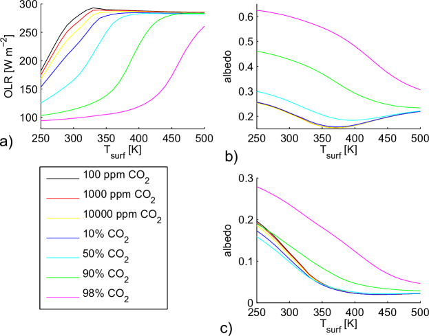
Figure 3: a) OLR as a function of surface temperature for various CO₂ dry volume mixing ratios, with fixed $T_{strat}=200$ K, 100% relative humidity, and Earth gravity and present-day atmospheric nitrogen inventory. b, c) Corresponding planetary albedo for G- and M-star incident spectra, respectively.

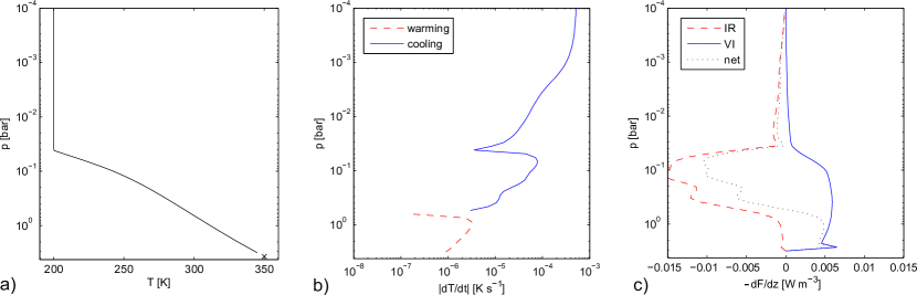
Figure 5: a) Temperature profile, b) radiative heating rates and c) flux gradients for an atmosphere with Earth’s present day N₂ inventory, CO₂ dry volume mixing ratio of 0.7, solar forcing of 0.85$F_{0}$, RH=1.0, $T_{surf}=350$ K and fixed $T_{strat}=200$ K. The curves in b) and c) are related by $\frac{dT}{dt}=-\frac{dF}{dz}/\rho c_{p}$, with $\rho$ and $c_{p}$ as defined in the main text.

$r_{c}=GM_{p}/(2c_{s}^{2})$ the radius at the transonic point, $G$ the gravitational constant, $M_{p}$ the planetary mass, $c_{s}=\sqrt{\gamma_{H}R_{H}T_{base}}$ the isothermal sound speed, $\gamma_{H}$ and $R_{H}$ the adiabatic index and specific gas constant for atomic hydrogen, and $r_{b}$ and $n_{b}$ the radius and density of the base region. We took $M_{p}=M_{E}$ (Earth mass) in most cases and assumed $n_{b}$ to be the total density at the homopause. In highly irradiated atmospheres, heating can increase the planetary cross-section in the XUV and hence the total amount of radiation absorbed. We crudely account for this effect here by assuming a radius $r_{XUV}=1.3r_{E}$ for absorption of XUV by H ionization (with $r_{E}$ Earth’s radius). Reference to calculations that account for this effect shows that this is a reasonable assumption for a wide range of XUV forcing values (see e.g., Figs. 3 and 5 of Erkaev et al. (2013)). The assumption that $n_{b}$ is the total homopause density overestimates the hydrogen density and hence the total escape rate, but the error due to this is reduced by the fact that the hydrogen scale height is a factor of 18 (44) larger than that of H₂O (CO₂). As a result, an escaping upper layer of atomic hydrogen may remain in thermal contact with the heavier gases below but decrease in density relatively slowly. We also neglect hydrodynamic drag of these gases on the hydrogen, which again leads us to overestimate escape rates when the incoming UV flux is high.

Finally, to couple the climate and loss rate calculations in time, it was necessary to incorporate the evolution of total stellar luminosity. For this, we assumed no variation for M-stars (constant $L=0.025L_{\sun}$), and evolution for G-stars according to the expression

$$F=F_{0}\left(1+\frac{2}{5}\left(1-t/t_{0}\right)\right)^{-1}$$ (13)

given in Gough (1981), with $F_{0}$ the present day solar flux and $t_{0}=4.57$ Gy.

3 Results

3.1 Variation of OLR and albedo with surface temperature and CO₂ mixing ratio

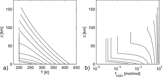
Figure 2: a) Temperature and b) H₂O volume mixing ratio vs. altitude for tests with fixed stratospheric temperature, 1 bar background N₂ and no CO₂. Profiles finish at a minimum pressure level $p_{min}=1$ Pa.

We first compared the results of our model with the classical runaway greenhouse calculations of Kasting (1988). For this we assumed 1 bar of N₂ as the background incondensible gas and a constant stratospheric temperature of 200 K. Figure 2 shows the temperature profiles and H₂O volume mixing ratios obtained. The results are almost identical to those in Kasting (1988), demonstrating that the inclusion of the non-ideality terms discussed in Section 2 makes little difference to the results for this range of surface pressures. Computing the outgoing longwave radiation for this set of profiles, we found a peak of 296 W m^-2, compared with $\sim 310$ W m^-2 in Kasting (1988) (results not shown). This is close to the value reported in Pierrehumbert (2010), which is unsurprising because the H₂O continuum dominates the OLR in the runaway limit..

Next, we calculated the OLR and albedo vs. surface temperature for a range of CO₂ dry volume mixing ratios. Figure 3 shows a) the OLR and b,c) albedo for G- and M-star spectra, respectively, assuming Earth’s gravity and present-day atmospheric nitrogen inventory. For intermediate surface temperatures, carbon dioxide reduces the OLR, but by $T_{surf}\sim 500$ K, the runaway limit is approached by all cases except the 98% CO₂/2% N₂ atmosphere. At high temperatures, the limiting OLR varies between 285.5 W m^-2 (100 dry ppm CO₂) and 282.5 W m^-2 (50% dry CO₂). This is in close agreement with the line-by-line calculations of Goldblatt et al. (2013); use of the HITEMP 2010 database for H₂O would probably have resulted in a reduction in our limiting OLR by a few W m^-2.

CO₂ also has a important effect on the planetary albedo, particularly in the G-star case, with a stronger influence at higher temperatures than for the OLR. This can be explained by the fact that all the atmospheres are more opaque in the infrared than in the visible, so CO₂ continues to affect the visible albedo even at high temperatures, when the H₂O column amount becomes extremely high.

Our planetary albedo values are systematically lower than those in Kasting (1988), as was also found by Kopparapu et al. (2013) in their recent (cloud-free) revision of the inner edge of the habitable zone. This is caused by atmospheric absorption of H₂O in the visible, due to vibrational-rotational bands that were poorly constrained when the radiative-convective calculations in Kasting (1988) were performed, but are included in the HITRAN 2008 database (Rothman et al., 2009). The effects of this absorption beyond simple changes in the planetary albedo are discussed in detail in the next section.

3.2 Shortwave absorption and low atmosphere temperature inversions

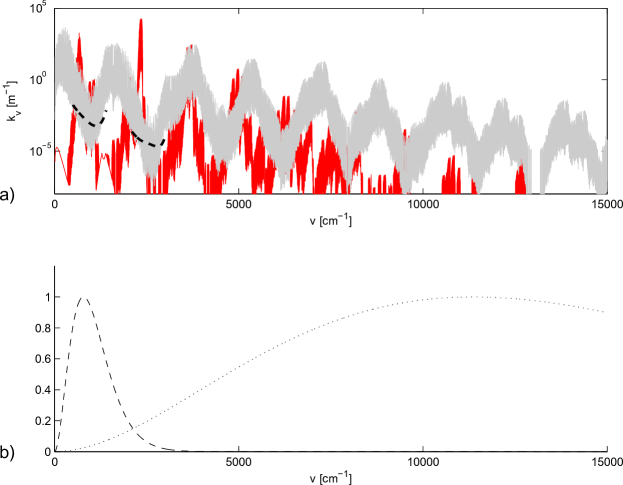
Figure 4: a) High-resolution absorption data for CO₂ (red) and H₂O (gray) used to create correlated-$k$ coefficients for the radiative transfer calculations. Data shown are for pure gas absorption at 400 K and 0.1 bar. The H₂O continuum [as defined in Pierrehumbert [2010]] is indicated by the dashed black lines. b) Normalised blackbody emission at $T=400$ K and 5800 K (dashed and dotted lines, respectively).

The absorption spectra of CO₂ and H₂O from the far-IR to 0.67 $\mu$ m are shown in Fig. 4 a). For comparison, blackbody curves at 400 and 5800 K are shown in Fig. 4 b). As can be seen, the absorption bands of both gases extend well into the visible spectrum. As a result, when a terrestrial planet’s atmospheric CO₂ content is high, the amount of starlight reaching the surface is greatly reduced. When the atmosphere is thick enough, this can qualitatively change the net radiative heating profile in the atmosphere. In Fig. 5, the temperature profile, radiative heating rates and flux gradients are plotted for a planet with Earth-like gravity and atmospheric N₂ inventory, CO₂ dry volume mixing ratio of 0.7, $T_{surf}=350$ K and fixed $T_{strat}=200$ K, irradiated by a G-class (Sun-like) star. As can be seen, the visible absorption by CO₂ and H₂O is strong enough to cause net heating, rather than cooling, in the lower atmosphere.

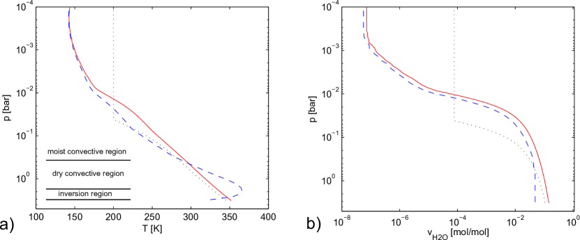
Figure 6: a) Temperature profiles and b) H₂O volume mixing ratios for the same atmospheric composition as in Fig. 5. Red solid (blue dashed) curves are for cases where departure from the moist adiabat was inhibited (permitted) in the low atmosphere (below 0.2 bar). The black horizontal lines and text on the left indicate atmospheric regions for the blue dashed curve.

To examine the effect of this heating on the atmospheric temperature profiles, we ran the radiative-convective model in time-stepping mode until a steady state was reached (Fig. 6). In one simulation, we allowed the atmosphere to evolve freely (red line), while in another, we forced the temperature profile to match the moist adiabat below 0.2 bar. For this example, cloud effects were neglected in the calculation of the visible albedo. As can be seen, in both iterative cases, CO₂ cooling in the high atmosphere reduces stratospheric temperatures to around 150 K, significantly decreasing $f_{H_{2}O}$ there. This effect is discussed further in the next section. In addition, in the freely iterative case, the low atmospheric absorption causes a strong temperature inversion to form near the surface. Above the inversion region, the atmosphere again becomes convectively unstable, following the dry adiabat as pressure decreases until the air is once again fully saturated, after which the model returns the temperature profile to the moist adiabat. The resulting reduction in surface temperature and lowered relative humidity ($RH$) in the inversion layer causes $f_{H_{2}O}$ to decrease slightly more in the upper atmosphere compared to the case where the lower atmosphere was forced to follow a moist adiabatic temperature profile.

We chose this high-CO₂ example to give a clear demonstration of the phenomenon, but this pattern of cooling in the mid-atmosphere but heating at depth should be an inevitable feature of very moist atmospheres around main sequence stars. Because the H₂O continuum region between 750 and 1200 cm^-1 (see Fig. 4) is the ultimate limiting factor on cooling to space when H₂O levels are high, the peak region of IR cooling becomes fixed around 0.1 bar (see Fig. 5) once the atmosphere is sufficiently moist. However, absorption by both H₂O and CO₂ is weaker per unit mass in the shortwave than in the longwave, so most stellar absorption must occur deep in the atmosphere, where the high IR opacity means that radiative cooling rates are low. Low atmosphere heating is generally even stronger around M-stars than G-stars, because the red-shift in the stellar radiation increases absorption and decreases the importance of Rayleigh scattering (e.g., Kasting et al., 1993; Wordsworth et al., 2010b).

Further understanding of the inversion behaviour can be gained by considering the surface energy budget. Because some radiation still reaches the ground even at very high CO₂ levels, evaporation of H₂O from the surface will still occur whenever a surface liquid source is present. In fact, when the temperature of the low atmosphere is higher than that of the ground, evaporation must increase, as evidenced by the equilibrium surface energy equation

$$F_{L}=F^{sw}_{abs}+c_{p}\rho_{a}C_{D}\|{\bf v}_{\rm a}\|(T_{a}-T_{surf})+\sigma\left(T_{a}^{4}-T_{surf}^{4}\right).$$ (14)

Here $F^{sw}_{abs}$ is the incident shortwave radiation from above absorbed by the surface, $C_{D}$ is a drag coefficient and $\rho_{a}$, $T_{a}$ and $\|{\bf v}_{\rm a}\|$ are the atmospheric density, temperature, and mean wind speed near the surface, and it is assumed that the lower atmosphere is optically thick in the infrared. Clearly, $F_{L}$, the latent heat flux due to evaporation, must be positive to balance the right hand side if $T_{a}>T_{surf}$. This immediately implies a net loss of mass from the surface as liquid is converted to vapour.

In a steady state, the mass loss due to evaporation must be balanced by precipitation. However, in the regions where the atmosphere undergoes net radiative heating, $RH$ drops below unity, so evaporation of precipitation should lead to a mass imbalance in the hydrological cycle and hence a net increase in the atmospheric mass over time. If the atmosphere were well-mixed everywhere, this process would continue until the temperature inversion was removed and moist convection could presumably again occur in the low atmosphere.

In reality, the picture is more complex, because convective and boundary layer processes lead to frequent situations where $RH$ varies significantly even on small scales (Pierrehumbert et al., 2007). The large-scale planetary circulation is also important: on the present-day Earth, broad regions of downwelling in the descending branches of the Hadley cells have $RH$ well below 1.0. Interestingly, recent general circulation model (GCM) simulations of moist atmospheres near the runaway limit have also shown evidence of temperature inversions, although so far only for the special case of tidally locked planets around M-stars (Leconte et al., 2013).

In the following analysis, to bracket the uncertainty in the results, we show cases where the atmosphere was allowed to evolve freely alongside those where the atmosphere was forced to follow the moist adiabat in the lower atmosphere. For the latter simulations, we simply switched off shortwave heating deeper than a given pressure (here, 0.2 bar), while still requiring balance between net outgoing and incoming radiation at the top of the atmosphere in equilibrium. As will be seen, the surface temperatures and cold-trap H₂O mixing ratios tended to be lower when the atmosphere evolved freely. The general issue of atmospheric temperature inversions due to shortwave absorption in dense moist atmospheres is something that we plan to investigate in more detail in future using a 3D model. It is likely to be particularly important for planets around M-stars, which have elevated atmospheric absorption due to their red-shifted stellar spectra.

3.3 Dependence of upper atmosphere H₂O mixing ratio on CO₂ levels

Before performing iterative calculations of the cold-trap temperature, we first calculated the dependence of the upper atmospheric H₂O mixing ratio on CO₂ levels assuming a fixed (high) stratospheric temperature of $T_{strat}=200$ K. This is close to the skin temperature for Earth today: assuming an albedo of 0.3, $T_{skin}=2^{-1/4}\left(OLR/\sigma\right)^{1/4}=214$ K. However, as should be clear from the iterated profiles in Figure 6, it represents a considerable overestimate when the main absorbing gas in the atmosphere is non-gray. As previously mentioned, carbon dioxide is particularly effective at cooling the high atmosphere because its strong 15 $\mu$m absorption band remains opaque even at low pressures.

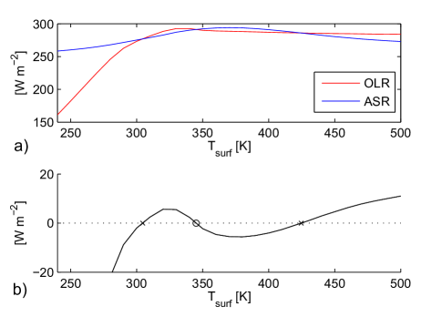
Figure 8: a) OLR, ASR and b) OLR - ASR for an atmosphere with three thermal equilibria (two stable solutions shown by crosses, one unstable solution shown by the circle). For this example, $F=1.025F_{0}$ and the CO₂ dry volume mixing ratio was 100 ppm.

Figure 7a) (left) shows the surface temperature as a function of CO₂ surface partial pressure $p_{CO_{2}}$, for a range of solar forcing values, assuming the planet is Earth and the star is the Sun. When the incoming solar radiation was close to the runaway limit, multiple equilibria were found for some $p_{CO_{2}}$ values. This was due to the varying behaviour of OLR and albedo with temperature (see Fig. 8). In the following analysis, we take the hottest stable solution whenever multiple equilibria are present, in keeping with our aim of a conservative upper limit on stratospheric moistening.

Figure 7a) (right) shows the corresponding mixing ratio of H₂O at the cold-trap $f_{H_{2}O}^{trap}$ for the same range of cases, with the high $T_{surf}$ solution chosen when multiple equilibria were present. As can be seen, increasing CO₂ initially moistens the atmosphere at the cold trap by increasing surface temperature. This effect continues until $p_{CO_{2}}\sim 0.1$ bar, after which the cold-trap fraction of H₂O declines again, despite the continued increase in surface temperature. Deeper insight into this phenomenon can be gained by studying a semi-analytical model. Equation (5) can be simplified in the ideal gas, constant $L$ and $c_{V,n}$ limit to

$$\frac{\mbox{d ln }\alpha_{v}}{\mbox{d }T}=\frac{\left(\alpha_{v}+\epsilon\right)/T-c_{p,n}/L}{\alpha_{v}+R_{n}T/L},$$ (15)

assuming that the relationship between $\rho_{v}$ and $T$ is given by the Clausius-Clayperon equation. Here $\epsilon=m_{v}/m_{n}$ is the molar mass ratio of the condensing and non-condensing atmospheric components. In the limit $\alpha_{v}\to\infty$, (15) is trivially integrated from the surface to cold trap to yield

$$\frac{\alpha_{v,trap}}{\alpha_{v,surf}}\sim\frac{T_{trap}}{T_{surf}}$$ (16)

Conversely, in the limit $\alpha_{v}\to 0$, (15) integrates to

$$\frac{\alpha_{v,trap}}{\alpha_{v,surf}}\sim\mbox{exp}\left[{+\frac{L}{R_{v}}\left(T_{surf}^{-1}-T_{trap}^{-1}\right)}\right]\left(\frac{T_{surf}}{T_{trap}}\right)^{c_{p,n}/R_{n}}.$$ (17)

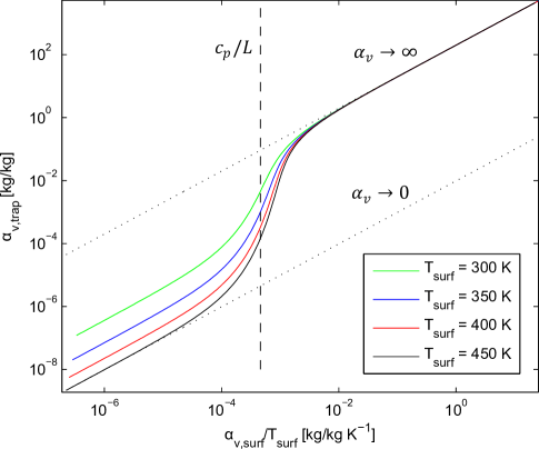
Figure 9: Condensible to non-condensible mass mixing ratio at the cold-trap $\alpha_{v,trap}$ vs. $\alpha_{v,surf}/T_{surf}$ according to (15), for a range of $T_{surf}$ values and $T_{strat}=200$ K. The transition to a moist stratosphere occurs for a narrow range of $\alpha_{v,surf}/T_{surf}$ values centered around $c_{p,n}/L$ (dashed line). The behaviour of $\alpha_{v,trap}$ in the limits $\alpha_{v,surf}\to\infty$ and $\alpha_{v,surf}\to 0$ (for $T_{surf}=450$ K) are shown by the dotted lines.

For temperature ranges and $L$, $c_{p}$ values appropriate to H₂O condensation in an N₂/CO₂ atmosphere, the transition between these two limits occurs rapidly over a small range of $\alpha_{v}$ values. Figure 9 a) shows $\alpha_{v,trap}$ as a function of $\alpha_{v,surf}$ given $T_{surf}=350$ K and $T_{trap}=150$ K in a pure N₂ atmosphere. As can be seen, $\alpha_{v,trap}$ only deviates from the lower and upper limits in a relatively narrow region. With reference to (15), we can define a dimensionless moist saturation number

$$\mathcal{M}\equiv\frac{\rho_{v,surf}L}{\rho_{n,surf}c_{p,n}T_{surf}}.$$ (18)

based entirely on surface values. As Fig. 9 shows, the transition to a regime where the upper atmosphere is moist occurs when $\mathcal{M}>1$. Equivalently, saturation of the upper atmosphere becomes inevitable once the latent heat of the condensible component at the surface exceeds the sensible heat of the non-condensing component. Because of the nonlinearity of the transition between the two regimes, this general scaling analysis can still be used as a guide even when $T_{trap}$ varies, although for quantitative estimates of $\alpha_{v,trap}$ near $\mathcal{M}=1$, numerical calculations are required, as should be clear from Fig. 7.

Assuming a saturated moist adiabat, this definition of $\mathcal{M}$ allows us to derive an expression for the rate at which $T_{surf}$ must increase with $p_{CO_{2},surf}$ in order for the upper atmosphere to remain moist. Given

$$p_{n,surf} = \epsilon\frac{p_{sat}(T_{surf})}{\alpha_{v,surf}}$$ (19)

$$= \frac{\epsilon Lp_{sat}(T_{surf})}{c_{p,n}T_{surf}\mathcal{M}}$$ (20)

then

$$p_{n,surf}(\mathcal{M}=1)=\frac{\epsilon Lp_{0}}{c_{p,n}}\frac{\mbox{exp}\left[{-\frac{L}{R_{v}}\left(T_{surf}^{-1}-T_{0}^{-1}\right)}\right]}{T_{surf}}$$ (21)

and hence

$$p_{CO_{2},surf}(\mathcal{M}=1)=\frac{\epsilon Lp_{0}}{c_{p,n}}\frac{\mbox{exp}\left[{-\frac{L}{R_{v}}\left(T_{surf}^{-1}-T_{0}^{-1}\right)}\right]}{T_{surf}}-p_{N_{2},surf}.$$ (22)

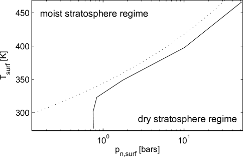
Figure 10: Surface temperature as a function of non-condensible surface partial pressure $p_{n,surf}$ (N₂ and CO₂) given a solar flux $F=0.9F_{0}$ (solid line) and assuming fixed $T_{strat}=200$ K. The dashed line shows the $\mathcal{M}=1$ temperature limit derived from (21). The initial rapid increase of $T_{surf}$ with $p_{n,surf}$ occurs due to the addition of CO₂ in small quantities to an initially N₂-dominated atmosphere.

The curve described by (21) is plotted in Fig. 10 alongside the actual increase of temperature with $p_{n,surf}$ for a simulation with $F=0.9F_{0}$ and variable CO₂, for comparison. When CO₂ is a minor component of the atmosphere, its greenhouse effect per unit mass is high, so increasing its mixing ratio raises surface temperatures but barely affects $p_{n,surf}$. However, once CO₂ is a major constituent, it begins to significantly contribute to $p_{n,surf}$ and hence to the sensible heat content of the atmosphere. In addition, it begins to increases the planetary albedo via Rayleigh scattering (Fig. 3b). Then, the increase of $T_{surf}$ with $p_{n,surf}$ is no longer sufficient to allow the climate to cross over into the moist stratosphere regime, and the H₂O mixing ratio in the upper atmosphere again declines. We have focused here on CO₂ and H₂O, but the analysis described is quite general and would apply to any situation where an estimate of a condensible gases’ response to addition of a non-condensible greenhouse gas is required.

Having established that we understand the fundamental behaviour of the model, we now turn to the cases where some or all of the atmosphere is allowed to evolve freely. Fig. 7b) shows the cases where the temperature profile was fixed to the moist adiabat below 0.2 bar but allowed to evolve freely in the upper atmosphere. Broadly speaking, surface temperatures are similar to the $T_{strat}=200$ K case. However, for low values of the stellar forcing $F$, $f_{H_{2}O}^{trap}$ is significantly lower, due to CO₂ cooling in the upper atmosphere. The transition to a warm, saturated stratosphere as $F$ is increased is nonlinear and rapid, due to near-IR absorption of incoming stellar radiation by H₂O.

When low atmosphere inversions were permitted, the behaviour of the system was more extreme. Fig. 7c) shows that in this case, $T_{surf}$ remains below 350 K for all values of $p_{CO2}$ until the solar flux is high enough for a runaway greenhouse state to occur. After this, no thermal equilibrium solutions were found for any $T_{surf}$ values between 250 and 500 K. As might be expected, the values of $f_{H_{2}O}^{trap}$ were correspondingly low in the pre-runaway cases. Temperature differences between the surface and warmest regions of the atmosphere reached $\sim$70 K in the most extreme scenarios (i.e., high $p_{CO_{2}}$, high $F$).

For the M-star case, we found broadly similar stratospheric moistening patterns as a function of $F$. The transition to a moist stratosphere tended to occur at lower $F$ values due to the decreased planetary albedo and increased high atmosphere absorption of stellar radiation, although trapping was effective at very high $p_{CO_{2}}$ levels. In addition, when lower atmosphere temperature inversions were permitted, they were typically even stronger than in the G-star case.

3.4 Sensitivity of the results to cloud assumptions

Up to this point, we have entirely neglected the effects of clouds on the atmospheric radiative budget. Clouds play a key role in the climates of Earth, past and present (Goldblatt and Zahnle, 2010; Hartmann et al., 1986) and Venus (Titov et al., 2007). However, their effects are extremely hard to predict in general, due to continued uncertainty in microphysical and small-scale convective processes. Here, to get a estimate of their effects on our main conclusions, we performed a sensitivity study involving a single H₂O cloud layer with 100% coverage of the surface and an atmosphere with the same composition, temperature profile and stellar forcing as in Fig. 6. CO₂ clouds would not form in the atmospheres we are discussing because the temperatures are too high to intersect the CO₂ vapour-pressure curve at any altitude.

As Fig. 14 shows, the net radiative forcing vs. the clear-sky case due to the presence of clouds is negative over a wide range of conditions. Only high clouds have a significant effect on the OLR, because at depth the longwave radiative budget is dominated by H₂O and CO₂ absorption at all wavelengths. However, high clouds are also more effective at increasing the planetary albedo. To have a warming effect, high clouds must be composed of particles that are large enough to effectively extinguish upwelling longwave radiation without significantly increasing the albedo. While this is not inconceivable, the extent of such clouds is likely to be limited due to the low residence times of larger cloud particles and lower rate of condensation in the high atmosphere.

Hence adding a more realistic representation of clouds would most likely lower surface temperatures compared to the clear-sky simulations we have discussed. This would cause even lower predictions of the H₂O mixing ratio at the cold trap, which is in keeping with our aim of estimating the upper limit for water loss as a function of $p_{CO_{2}}$. In this sense, our results are in line with previous studies, particularly Kasting (1988), who also tested the effects of clouds in their model and came to similar conclusions about their effect on climate. Some improvement in cloud modeling can be provided by 3D planetary climate simulations (e.g., Wordsworth et al., 2011), which allows the effects of the large-scale dynamics to be taken into account. However, fundamental assumptions on the nature of the cloud microphysics are still necessary in any model. Hence studies that constrain cloud effects rather than predicting them are likely by necessity to be the norm for some time to come.

3.5 Effects of changing atmospheric nitrogen content

Because of the random nature of volatile delivery to planetary atmospheres during and just after formation, it is also interesting to consider the variations in H₂O loss rates that occur when the N₂ content of a planet varies. Like H₂O and CO₂, nitrogen affects the radiative properties of the atmosphere, through collision broadening and collision-induced absorption (CIA) in the infrared and Rayleigh scattering in the visible. These effects tend to partially cancel out, with the result that the effect of doubling atmospheric N₂ on Earth is a small increase in surface temperature (Goldblatt et al., 2009). Hydrogen-nitrogen CIA can cause efficient warming in cases when the hydrogen content of the atmosphere is greater than a few percent (Wordsworth and Pierrehumbert, 2013), but we will not consider such scenarios further here.

When CO₂ levels are high, N₂ warming can be much more significant, because its effectiveness as a Rayleigh scatterer is less than that of CO₂. Fig. 13 shows that a fivefold increase in the atmospheric nitrogen inventory of an Earth-like planet can cause large surface temperature increases at high $p_{CO_{2}}$. Nonetheless, in terms of the cold-trap H₂O mixing ratio, the thermodynamic effects of N₂ are most critical. As should be clear from (21), an increase in the partial pressure of the non-condensible atmospheric component means a higher surface temperature is required to keep $f_{H_{2}O}^{trap}$ at the same value. Fig. 13 shows that with $5\times$ PAL atmospheric N₂, an Earth-like planet would have a significantly drier stratosphere despite the increase in surface temperature for $p_{CO_{2}}>$0.3 bar.

Conversely, if N₂ levels are low, upper atmosphere saturation and hence water loss can become extremely effective. In the limiting case where the N₂ and CO₂ content of the atmosphere is zero, efficient (UV energy-limited) water loss occurs at any surface temperature. Even an ice-covered planet with surface temperatures everywhere below zero could rapidly dissociate water and lose hydrogen to space if the atmosphere was devoid of non-condensing gases. Such a scenario would likely be short-lived on an Earth-like planet, because CO₂ would quickly accumulate in its atmosphere due to volcanic outgassing. This would not be the case if the planet’s composition was dominated by H₂O, as in the ‘super-Europa’ scenarios discussed in Pierrehumbert (2011). In this situation, however, there would be no obvious sink for O₂ generated by H₂O photolysis, so an oxygen atmosphere would presumably accumulate. This could eventually limit water loss by the cold-trap mechanism, although we note that without CO₂ cooling, an O₂-dominated upper atmosphere could reach extremely high temperatures. This issue has implications for the search for life on other planets, because oxygen is frequently considered to be a biomarker gas (e.g., Selsis et al., 2002). We leave the pursuit of this interesting problem for future research.

Finally, surface gravity affects stratospheric H₂O mixing ratios in predictable ways. Increased $g$ leads to higher $p_{n,surf}$ for a given atmospheric N₂ inventory, reducing $\mathcal{M}$ and hence stratospheric moistening for a given surface temperature. Note, however, that the effect of this on water loss is partially mitigated by the fact that scale height decreases with gravity, and hence diffusion-limited H₂O loss rates increase [see (6)].

3.6 Water loss due to impacts

The final modifying effect we considered was heating due to meteorite impacts. Impacts have been studied in the context of early Venus, Earth and Mars in terms of their potential to cause heating and modification of the atmosphere and surface (Zahnle et al., 1988; Abramov and Mojzsis, 2009; Segura et al., 2008). Delivery of volatiles by impactors during the late stages of planet formation is also of course a major determinant of a planet’s final water inventory, as we discussed in the Introduction. Here, our aim is simply to estimate whether impact heating could modify our conclusion that cold-trapping of H₂O strongly limits water loss for most values of $p_{CO_{2}}$. First, we calculate the impactor energy required to moisten the stratosphere for a given starting composition and surface temperature. We then compare this value with the critical energy required for an impactor to cause substantial portions of the atmosphere to be directly ejected to space. In the interests of getting an upper limit on water loss, we ignore the potential for ice-rich impactors to deliver H₂O directly to the surface.

We assume that for an impactor of given mass and velocity, a portion $\varepsilon E_{K}$ of the total kinetic energy $E_{K}$ per unit planetary surface area will be used to directly heat the atmosphere (Fig. 15). Accounting for the sensible and latent enthalpy $E_{sens}$ and $E_{lat}$, the total energy of an atmosphere per unit surface area can be written as

$$E_{tot} = E_{sens}+E_{lat}$$ (23)

$$= \frac{1}{g}\int^{p_{surf}}_{0}\left(c_{p}T+q_{v}L\right)\mbox{d}p$$ (24)

if we assume that the contribution of any condensed material is small and neglect the latent heat of ‘incondensible’ components like N₂ and CO₂. Here $c_{p}$ is the mean constant-pressure heat capacity and $q_{v}=(m_{v}/\overline{m})f_{v}$ is the mass mixing ratio of the condensable component (H₂O), with $\overline{m}$ the (local) mean molar mass of the atmosphere.

To the level of accuracy we are interested in, the initial atmospheric energy can be approximated from (24) as

$$E_{tot}=E_{0}\sim\frac{c_{p,n}T_{surf}p_{n,surf}}{g}+\epsilon Lp_{v}(T_{surf})/g,$$ (25)

We now wish to calculate the threshold energy input necessary to push the atmosphere into a moist stratosphere regime. As shown previously, the transition occurs when $\mathcal{M}\sim 1$, and hence $E_{sens,n}\sim E_{lat}$. Given an atmospheric energy just after impact of $E_{1}(\mathcal{M}=1)$, the overall energy balance can be written

$$\varepsilon E_{K} = E_{1}(\mathcal{M}=1)-E_{0}$$ (26)

$$= 2E_{lat}(T_{surf}^{*})-\frac{c_{p,n}T_{surf}p_{n,surf}}{g}-\frac{\epsilon Lp_{v}(T_{surf})}{g}.$$ (27)

Given $\mathcal{M}=1$, from (18) we have the transcendental equation $\epsilon p_{v}(T_{surf}^{*})L=p_{n,surf}c_{p,n}T_{surf}^{*}$. This can be solved for $T_{surf}^{*}$ for a given $p_{n,surf}$ by Newton’s method, assuming 100 % relative humidity at the surface. This then allows $\epsilon E_{K}$ to be calculated as a function of $p_{n,surf}$ and $T_{surf}$.

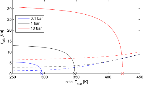
Figure 16: Critical impactor radius necessary to cause transition to a $\mathcal{M}=1$ moist stratosphere regime assuming 100% energy conversion efficiency (solid lines), and to cause significant atmospheric erosion to space (dashed lines). Colors indicate the partial pressure of the incondensible gas (assumed 100% CO₂ here for simplicity). Crosses at the base of the plot indicate the temperature $T_{surf}^{*}$ at which $\mathcal{M}=1$. The increase of the critical erosion radius with $T_{surf}$ is due to its dependence on the scale height of the atmosphere.

In Fig. 16, the minimum impactor radius $r_{crit}$ required to cause a transition to the moist regime is plotted vs. initial surface temperature $T_{surf}$, for three CO₂ partial pressures, assuming 100% energy conversion efficiency ($\varepsilon=1$), a mean impactor density of $\rho_{i}=3$ g cm^-3, and an impact velocity equal to Earth’s escape velocity. For simplicity, N₂ is neglected and the Clausius-Clayperon equation is used for $p_{v}$. Alongside this, the critical radius for erosion of a significant portion of the atmosphere $r_{erode}$ is also shown. The latter quantity can be defined as the radius required for removal of a tangent plane of the atmosphere (Ahrens, 1993) such that

$$r_{erode}=\left(\frac{3}{4\pi}\frac{\rho_{a}}{\rho_{i}}H_{s}^{2}r_{p}\right)^{\frac{1}{3}}$$ (28)

where $\rho_{a}$ and $H_{s}$ are representative density and scale height values for the atmosphere and $r_{p}$ is the planetary radius. In Fig. 15, we use surface values for $\rho_{a}$ and $H_{s}$ to get an upper limit for $r_{erode}$.

As can be seen, the critical erosion radius is significantly smaller than the radius required to create a moist upper atmosphere except when the initial surface temperature is very close to the value at which $\mathcal{M}=1$. It is therefore almost impossible for atmospheres to be forced into a moist stratosphere regime by impact heating without significant erosion also occurring. Erosion will remove a fraction of the incondensible atmospheric component of order $\frac{1}{4}H_{s}/r_{p}$, and has the side-effect of also making it possible for smaller subsequent impactors to cause erosion. Without any further calculation, it is therefore clear that impacts will only cause substantial water loss if they also remove significant amounts of CO₂ and/or N₂ from the planet’s atmosphere.

Interestingly, Genda and Abe (2005) argued that impact erosion on planets with oceans may be quite efficient, because of the expansion of hot vaporised H₂O and reduced shock impedance of liquid water compared to silicate materials. Clearly, if this mechanism reduced atmospheric CO₂ or N₂ to extremely low levels post-formation on an ocean planet, water loss could then become rapid, as described in Section 3.5. However, while ocean-enhanced erosion may have been important for removing much of Earth’s primordial atmosphere when it formed, it clearly allowed substantial amounts of N₂ and CO₂ to remain, as evidenced by the significant total present-day inventories of these volatiles. For higher mass planets, it is therefore still plausible that large volatile inventories remain in the period immediately following the late stages of oligarchic growth.

3.7 Escape rate in moist stratosphere ($\mathcal{M}>>1$) limit

So far, we have only considered processes that affect water loss by modifying the saturation of H₂O at the cold trap. To complete the analysis, we now discuss constraints on the rate of H escape when the cold-trapping of H₂O in the stratosphere is no longer a limiting factor. The first constraint we considered was the maximum possible photolysis rate of H₂O. We estimated this by calculating the integral

$$\phi_{photo}=\int_{0}^{\lambda_{cut}}Q_{y}(\lambda)F(\lambda)\mbox{d}\lambda$$ (29)

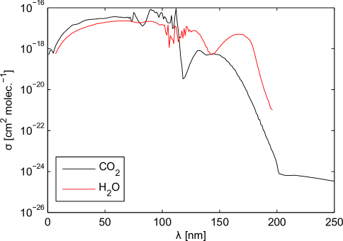
Figure 12: CO₂ and H₂O absorption cross-sections in the UV used in the model, as a function of wavelength.

where $F(\lambda)$ is the net stellar flux per unit area of the planet’s surface, $Q_{y}$ is the quantum yield of the reaction H2O + hν→H + OH and $\lambda_{cut}=196$ nm is the wavelength beyond which UV absorption by H₂O is negligible (see Fig. 12). For present-day values of the solar UV spectrum we calculated $\phi_{photo}=2\times 10^{12}$ molecules cm^-2 s^-1. This corresponds to a rapid water loss rate of 3.2 Earth oceans Gy^-1, which would be even higher under elevated XUV/UV flux conditions. We tested the dependence of this limit on the CO₂ mixing ratio in the upper atmosphere, but found that CO₂ had little shielding effect when H₂O was a significant atmospheric component, because the cross-section of H₂O is higher in the UV region (see Figs. 12 and 17b).

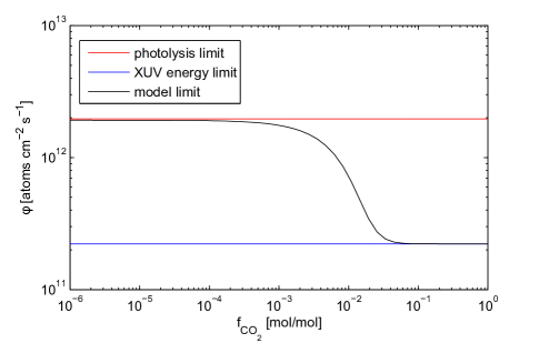
Figure 17: Hydrogen (H) escape rate as a function of CO₂ volume mixing ratio (molar concentration) for a CO₂/H₂O atmosphere under G-class stellar insolation with Sun-like XUV/UV spectrum.

Another limit on water loss in the saturated case can be found by considering the energy budget of the upper atmosphere. Figure 17 shows the results of a calculation based on the equations described in Section 2.3, with the exospheric temperature at each CO₂ mixing ratio value found by linear interpolation to solve (8) over a grid of values between 100 and 1000 K. In this example, we assumed a pure CO₂/H₂O upper atmosphere and synthetic solar UV spectrum appropriate to the present day, with an efficiency factor of 0.15 included in the XUV heating rate to incorporate photochemical and ionization effects (Kasting and Pollack, 1983; Chassefière, 1996). As can be seen, the CO₂ mixing ratio significantly affects the escape rate, with the energetic H loss limit slightly below the photolysis limit for low homopause $f_{CO_{2}}$ values, but decreasing to much lower values when CO₂ is a major constituent. Nonetheless, because we neglect cooling due to H₂O, the escape rates at low $f_{CO_{2}}$ values are probably unrealistically high. Adiabatic cooling of the escaping H, which is also neglected, is also important when the escape flux is high and would tend to cause lower values of $\phi_{hydro}$ than are shown here. Experimentation with different assumptions for $\phi_{hydro}(T_{base})$, including a conduction-free scheme that incorporates adiabatic cooling based on PiePierrehumbert2011BOOK, indicated that the value of $f_{CO_{2}}$ at which the escape rate begins to decrease to low values is likely overestimated in our model (results not shown). Nonetheless, our calculated XUV-limited escape rate of $\sim 2.2\times 10^{11}$ atoms cm^-2 s^-1 or $\sim 1\times 10^{30}$ atoms s^-1 is reasonably close to values found in vertically resolved escape models that assume similar initial conditions (e.g., Erkaev et al. (2013), Table 2). This indicates the ability of our approach to provide a basic upper limit on water loss in the presence of additional radiative forcing from UV absorption and IR emission.

When we increased the XUV/UV flux, the H escape rate rose correspondingly. The exospheric temperature also rose somewhat, but the efficiency of escape cooling under our isothermal wind assumption prevented it from exceeding 500 K even for a solar flux corresponding to 0.1 Ga. Under these extreme conditions, the escape rates in the model exceeded the photolysis limit even when CO₂ was abundant at the homopause. This result can be compared with the analysis of Kulikov et al. (2006), who calculated exospheric temperatures in a dry Venusian atmosphere that included the effects of conduction but neglected energy removal by atmospheric escape, and estimated that rapid hydrogen escape would occur for XUV fluxes $\sim 70\times$ present-day.

Our simple model allows several basic conclusions to be drawn regarding water loss in the moist stratosphere limit. First in agreement with Kulikov et al. (2006), we find that for planets receiving stellar fluxes that place them close to or over the runaway limit, such as early Venus, H removal could probably have been rapid even if CO₂ was abundant in the atmosphere. However, planets with CO₂-rich atmospheres around G-stars that receive a similar stellar flux to Earth can only experience significant UV-powered water loss early in their system’s lifetime. Around M-stars, XUV levels are elevated for much longer and the stellar luminosity is essentially unvarying with time, so more escape may occur if water vapour is abundant in the high atmosphere. The differences between G- and M-star cases and implications for terrestrial exoplanets in general are discussed further in the following section.

4 Discussion

4.1 H₂O loss rates vs. atmospheric CO₂ pressure

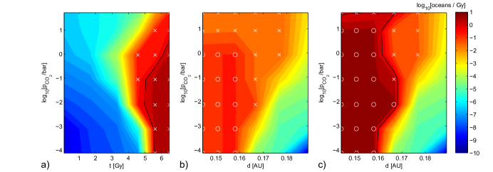
Figure 18: a) Water loss rate as a function of surface CO₂ partial pressure and time for an Earth-like planet around a G-star at 1 AU. Water loss rate as a function of surface CO₂ partial pressure and orbital distance for an Earth-like planet around b) a moderately active M3 class star (GJ 436) and c) a star with elevated Lyman-$\alpha$ emission. White crosses / circles indicate data points where escape was energy / photolysis rate limited, respectively. The solid black line indicates the contour for a loss rate of 1 Earth ocean Gy^-1.

To get an integrated view of water loss rates under a wide range of conditions, we used (6) in combination with (13) and the calculations discussed in the previous sections. In cases where the stellar flux was high enough to cause a runaway greenhouse, upper atmospheric $f_{H_{2}O}$ and $f_{CO_{2}}$ were calculated assuming a well mixed atmosphere and a total H₂O inventory of 1 Earth ocean for simplicity. The results in terms of Earth oceans per Gy are displayed in Figure 18 as a function of time/orbital distance and atmospheric CO₂. As can be seen, for the G-star case, water loss is diffusion-limited (and low) until late in the Sun’s evolutionary history, when surface temperatures increase sufficiently to allow a moist stratosphere at $p_{CO_{2}}$ values between 0.1 and 1 bar.

The fact that XUV and FUV fluxes decrease with time but total solar luminosity increases with time makes water loss from Earth-like planets around G-stars particularly hard to achieve. The faint young Sun effect causes strong limits on $f_{H_{2}O}$ at the cold trap early on for all values of $p_{CO_{2}}$. However, by the time total luminosity has increased enough to allow an H₂O-rich stratosphere at moderate $p_{CO_{2}}$ values, the planet is near the runaway greenhouse transition, and XUV and FUV fluxes have declined enough to make energy limitations important. For Earth, this suggests that factors such as a weaker magnetic field in the early Archean (Tarduno et al., 2010) are unlikely to have led to significant water loss compared to the present-day ocean volume. Hence despite the advances in radiative transfer modelling over the last few decades, the conclusions of Kasting and Ackerman (1986) remain essentially valid.

Around M-stars, the lack of temporal variation in total solar luminosity means water loss is most effective close to the inner edge of the habitable zone. However, the high and unpredictable variability in the XUV/UV flux is also important. In Fig. 18b), the escape rates are plotted assuming a synthetic UV spectrum appropriate to GJ 436, which is a relatively quiet M3 star. Fig. 18c) shows results for the same case, except with the 122 nm Lyman $\alpha$ emission line in the incident stellar spectrum scaled to the value for AU Mic, a young and active M1 star (Linsky et al., 2013). As can be seen, Lyman $\alpha$ variability can make a significant difference to water loss rates around M-stars both beyond and inside the runaway greenhouse threshold. Nonetheless, because of the cold trap constraints discussed in Section 3.3, high H₂O loss is never achieved for planets receiving total fluxes much less than that of Earth [approx. $d>0.17$ AU in Fig. 18c)]. The only effective way to enhance H₂O photolysis rates in these cases would appear to be via decreases in the total atmospheric non-condensible gas content.

Taken together, these results suggest that rocky exoplanets in the habitable zone may retain even a limited water inventory if they form with little H₂O, which is clearly a positive outcome from a habitability standpoint. Conversely, most planets that form with much more H₂O than Earth are unlikely to lose it via escape. Ocean planets may therefore be relatively common in general, which, as we discuss in the next section, has important implications for the search for exoplanet biosignatures.

For Venus, it might appear obvious from our calculations that the planet has always been in a runaway state. Indeed, our clear-sky calculations suggest Earth itself receives close to the limiting runaway flux at present, in agreement with the recent results of Goldblatt et al. (2013) and Kopparapu et al. (2013). When the Solar System formed, Venus received a solar flux $\sim 1.4$ times that of Earth today, apparently placing it well inside the runaway limit. However, our calculations neglect cloud radiative forcing and spatial variations in relative humidity, both of which can have a major effect on the runaway threshold. Using the present-day atmospheric CO₂ inventory (92 bars) and a solar flux $F=0.72F_{0}$ appropriate to 4.4 Ga, for early Venus we calculate that a negative radiative forcing of around 70 W m^-2 is needed to reach equilibrium surface temperatures of $\sim$320 K, at which point diffusion limits on H₂O escape are important. Hence while it is possible that clouds could have limited water loss from an early CO₂-dominated atmosphere, until their effects are understood in detail the argument that Venus lost its water early via rapid hydrodynamic escape (Gillmann et al., 2009) remains entirely plausible.

4.2 Climate and habitability of waterworlds

As described in Section 1, a planet with no subaerial land by definition will no longer experience land silicate weathering. For waterworlds, a large fraction of the total CO₂ inventory would then be expected to reside in the atmosphere and ocean, unless seafloor weathering were extremely effective. Partitioning of CO₂ between the atmosphere and ocean depends on carbonate ion chemistry and hence on the ocean pH, but in the absence of major buffering effects from other species, a large fraction of the total surface CO₂ inventory would still remain in the atmosphere for a planet with 10 times Earth’s ocean amount (see the Appendix for details). We have just shown that water loss rates in CO₂-rich atmospheres will be low for a wide range of conditions, so waterworlds could plausibly remain stable throughout their history. In the context of future searches for biosignatures on other planets [e.g., Kaltenegger et al. (2013)], therefore, it is interesting to consider the potential differences in habitability that are likely when no subaerial land is present.

Aside from the presence of liquid water, the first major consideration for the survival of life is surface temperature. If waterworlds do tend to have high atmospheric CO₂ inventories, those receiving an Earth-like stellar flux would have surface temperatures in the 350-450 K range. The survival range for life on Earth is around 250 to 400 K (Kashefi and Lovley, 2003), so a waterworld could perhaps still remain marginally habitable by this criterion unless other warming mechanisms were also present (see Figure 7).

Other constraints may come from the potential for life to emerge in the first place. It has been argued that life on Earth originated in shallow ocean or coastal regions, with evaporation cycles playing a key role in the development of a ‘primordial soup’ (Bada, 2004). Such a scenario would clearly be impossible on a planet with no exposed rock at the surface. Another leading hypothesis for the origin of life on Earth posits that it occurred in hydrothermal vents (specifically, in alkaline vents similar to the Lost City region in the mid-Atlantic) (Russell et al., 1994; Kelley et al., 2005). However, even this mechanism could become problematic if the ocean volume is so large that pressures at the seafloor are high enough to inhibit outgassing (e.g., Lammer et al., 2009).

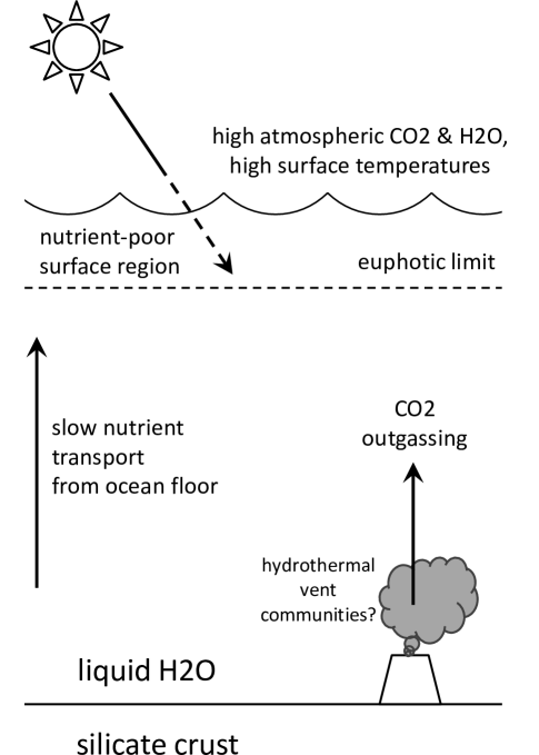
Figure 19: Schematic of processes affecting climate and biospheric productivity on a hypothetical Earth-like planet with oceans deep enough to cover the entire surface.

Finally, besides liquid water and an equable temperature range, all life on Earth requires certain essential nutrients (the so-called ‘CHNOPS’ elements plus a variety of metals). In the present-day oceans, net primary production is believed to be limited ultimately by the availability of phosphorous in particular, which is delivered primarily by weathering of exposed rock on the surface (Filippelli, 2008). Photosynthetic life in the ocean is restricted to the surface euphotic layer, but in the absence of a land source, elements like phosphorous, iron and sulphur could only be supplied there from the ocean floor, at rates that are typically 2-3 orders of magnitude smaller than comparable supply from the continents (Kharecha et al., 2005). An Earth-like biosphere on a waterworld would therefore have a net primary productivity that was several orders of magnitude lower than that of Earth today (see Figure 19). Given the strong selection pressures that would be present in such a nutrient-poor environment, it is conceivable that organisms dependent only on elements accessible from the atmosphere could develop. Nonetheless, these general considerations hint at some of the differences we should expect between land planets and ocean planets, as well as the subtlety of the relationship between water and habitability in general. Rather than simply extrapolating Earth-like atmospheric conditions and biospheric productivity, future biosignature studies should aim to investigate these issues in more detail.

4.3 Future work

There are a number of potential future research directions from this study. First, our results clearly indicate the need for a greater understanding of how the crust and mantle of Earth-like planets with high H₂O inventories evolve. Here, we have focused on the atmospheric component of the problem, but large uncertainties still remain regarding the exchange of CO₂ and H₂O between a planet’s mantle and surface. For CO₂, the high uncertainty in the physics and chemistry of seafloor weathering currently limits our ability to extrapolate Earth’s climate evolution to more general cases. This is a problem that would benefit greatly from more detailed observational and experimental constraints. For H₂O, partitioning between the surface and mantle is also still poorly understood (Hirschmann, 2006), although it has been hypothesized that if Earth’s ocean volume was lower, it would increase to the present value due to a feedback involving the ridge axis hydrothermal circulation (Kasting and Holm, 1992). If an (as yet unidentified) negative crust-mantle feedback also operates in the other direction, our conclusions regarding the potential abundance of ocean planets could require revision.

Regarding climate modeling, an obvious extension of this work is to examine the role of clouds and relative humidity variations in detail using a 3D climate model. For tidally locked planets around M-stars, in particular, the differences in the 3D case could be significant, because the nonlinear dependence of $f_{H_{2}O}^{trap}$ on stellar forcing means that the planet’s dayside stratosphere could be much more humid than a global mean calculation would suggest. We plan to assess the differences caused by the transition to 3D in future work. GCMs are also able to tackle cloud effects more accurately in principle, although as we have mentioned, uncertainties in sub-gridscale processes and cloud microphysics are not removed by 3D modeling. Selected numerical experiments using cloud-resolving models, perhaps combined with direct laboratory experiments on cloud microphysics under a range of non-Earth-like conditions, would be a valuable way to gain insight in future. Nonetheless, despite the uncertainties, the fact that clouds cool over most conditions relative to the clear-sky case means that they are unlikely to affect the robustness of our general conclusions here.

Observationally, we are still some way from being able to characterize low mass exoplanets of the type we have discussed, although the state of the art is advancing rapidly (Bean et al., 2010; Croll et al., 2011; Kreidberg et al., 2013). Both JWST and ESA’s planned EChO mission will be able to perform spectroscopic analysis of the atmospheres of nearby transiting super-Earths, which at minimum will allow the major optically active species in their atmospheres to be identified. However, to distinguish planets with volatile-rich atmospheres and high surface temperatures from more Earth-like cases, characterization of absorber abundances and surface pressures will be a key challenge. This can be done by transmission spectroscopy, in principle, as long as the planet’s atmosphere is clear enough in the visible at short wavelengths to allow identification of the spectral Rayleigh scattering slope (Benneke and Seager, 2012). Another promising approach that is valid for non-transiting planets is spectral phase curve analysis (Selsis et al., 2011), although the demands on instrumental sensitivity with this method are stringent. In the long term, detailed observational tests of planetary water loss theories will be best achieved via revival of NASA and ESA’s TPF/Darwin exoplanet characterization missions.

5 Acknowledgments

Photodissociation cross-section and quantum yield data and the solar spectrum in the UV were kindly provided by E. Hébrard at the Université de Bordeaux. The code used to compute the moist adiabat was partly based on routines originally provided by E. Marcq. For the M-star UV spectrum, we acknowledge use of the MUSCLES database. R. W. thanks Ty Robinson for enlightening intercomparisons with the SMART radiative code, and F. Ciesla, K. France, J. Linsky, R. Heller, D. Abbot and N. Cohen for discussions.

Appendix A Ocean / atmosphere partitioning of CO₂ on water-rich planets

To calculate the fraction of CO_2 stored in the ocean for a given atmospheric partial pressure, we calculated the chemical equilibria of the CO_2-carbonate-bicarbonate system, assuming contact with an infinite calcium carbonate reservoir following the methodology described in Pierrehumbert (2010). Chemical equations

$$\ce{CO_{2}(aq)+H_{2}O}\rightleftharpoons\ce{HCO_{3}^{-}+H^{+}}$$ (A1)

$$\ce{HCO_{3}^{-}}\rightleftharpoons\ce{CO_{3}^{2-}+H^{+}}$$ (A2)

and

$$\ce{CaCO_{3}(s)}\rightleftharpoons\ce{Ca^{2+}+CO_{3}^{2-}}$$ (A3)

were solved for a given pH by Newtonian iteration using the corresponding charge balance equation. Ocean CO_2(aq) was related to atmospheric $p_{CO_{2}}$ via Henry’s Law. Equilibrium and constants and their temperature dependencies were calculated from data in Tables 8.1 and 8.2 of Pierrehumbert (2010), while for the Henry’s Law coefficient, data from Carroll et al. (1991) was used. Finally, the ratio of atmospheric to ocean carbon content was calculated as

$$\mathcal{R}_{C}=\frac{K_{H}N_{CO_{2}(g)}}{p_{CO_{2}}N_{H_{2}O(l)}}\frac{1}{1+K_{1}\ce{[H^{+}]}^{-1}+K_{1}K_{2}\ce{[H^{+}]}^{-2}}$$ (A4)

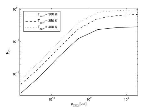
Figure 20: Ratio between total atmosphere and ocean inorganic carbon as a function of surface temperature and CO₂ partial pressure, for a predominately rocky super-Earth with 10 times Earth’s surface liquid water content, surface gravity $15$ m s^-2 and radius $1.3r_{E}$.

with $K_{1}(T)$ and $K_{2}(T)$ the equilibrium constants of (A1) and (A2), respectively, $K_{H}(T)$ Henry’s constant for CO_2, and $N_{H_{2}O(l)}$ and $N_{CO_{2}(g)}$ the total number of moles of H_2O in the ocean and CO_2 in the atmosphere, respectively. The latter quantity was calculated as a function of $p_{CO_{2}}$ and $T_{surf}$ using the atmospheric code described in the main text. Figure 20 shows $\mathcal{R}_{C}$ as a function of $p_{CO_{2}}$ for various ocean temperatures, for a hypothetical super-Earth exoplanet with $g=15.0$ m s^-2, total ocean amount 10 $\times$ that of Earth and radius $r_{P}=1.3r_{E}$.

As can be seen, $\mathcal{R}_{C}$ increases rapidly with $p_{CO_{2}}$ in all cases, increasing to over 0.1 for $p_{CO_{2}}>0.25$ bar at $T_{surf}=300$ K despite the increased ocean volume. $\mathcal{R}_{C}$ also significantly increases with temperature for all $p_{CO_{2}}$ values. This is primarily because $K_{H}$ (and hence CO₂ solubility) decreases with temperature, limiting the total amount of inorganic carbon the ocean can hold. This effect may be important for ocean planet climates in general: given the dependence of ocean temperatures on atmospheric CO_2 via the greenhouse effect, this should lead to a positive feedback on ocean planets between $p_{CO_{2}}$ and $T_{surf}$, which clearly will have a destabilizing effect. Because the solubility of many significant greenhouse gases decreases with temperature in water over wide ranges, similar positive feedbacks involving other gases could also be significant on ocean planets.

Figure 1: Schematic atmospheric temperature profile with the main processes influencing water photolysis and hydrogen loss in terrestrial planetary atmospheres indicated alongside. Transport of H₂O from the surface to upper atmosphere is limited by the cold trap. Hydrogen loss rates are controlled by the temperature of the upper atmosphere, which is primarily dependent on a balance between XUV and FUV absorption, IR emission, and the energy carried away by escaping particles.

Figure 7: (left) Surface temperature and (right) cold-trap H₂O volume mixing ratio as a function of surface CO₂ partial pressure for a range of incident solar fluxes. Cases a-c) are for simulations where a fixed stratospheric temperature of 200 K was assumed, where the temperature profile was fixed below 0.2 bar but evolved freely above, and where the entire atmospheric temperature profile evolved freely, respectively. In the latter case, strong temperature inversions formed near the surface due to shortwave H₂O absorption.

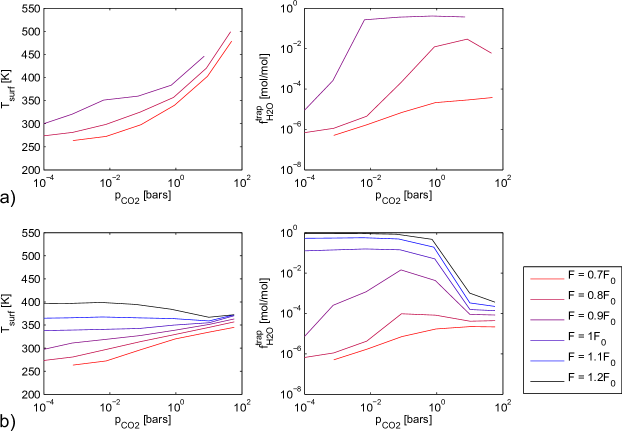
Figure 11: a-b) As for Figure 7b-c), but assuming an M-star incident spectrum. In cases where no data is shown, an equilbrium solution was not found for any surface temperature between 250 and 500 K.

Figure 13: a) Surface temperature and b) stratospheric H₂O volume mixing ratio as a function of surface CO₂ partial pressure, for simulations with varying surface gravity and total atmospheric nitrogen content.

Figure 14: Radiative effects of clouds for an atmosphere with the same composition, temperature profile and stellar forcing as shown in Fig. 5. a) Longwave and b) shortwave radiative forcing vs. the clear-sky case as a function of H₂O cloud particle radius, for a single layer with 100% coverage and opacity $\tau=1.0$ at 1.5 $\mu m$.

Figure 15: Schematic of the effect of an impact on a planet with a dense atmosphere. Some of the impactor kinetic energy is used to convert surface condensate material (here, liquid water) to vapour in the atmosphere. If the impactor radius is large enough, this may heat the atmosphere enough to moisten the stratosphere and allow transitory periods of rapid H₂O photolysis. However, large impactors will also cause substantial amounts of the atmosphere to be ejected to space.

References

- Abbot et al. (2012) D. S. Abbot, N. B. Cowan, and F. J. Ciesla. Indication of insensitivity of planetary weathering behavior and habitable zone to surface land fraction. The Astrophysical Journal, 178:756, 2012. 10.1088/0004-637X/756/2/178.
- Abe et al. (2011) Yutaka Abe, Ayako Abe-Ouchi, Norman H Sleep, and Kevin J Zahnle. Habitable zone limits for dry planets. Astrobiology, 11(5):443–460, 2011.
- Abramov and Mojzsis (2009) O. Abramov and S. J. Mojzsis. Microbial habitability of the Hadean Earth during the late heavy bombardment. Nature, 459:419–422, May 2009. 10.1038/nature08015.
- Ahrens (1993) Thomas J Ahrens. Impact erosion of terrestrial planetary atmospheres. Annual Review of Earth and Planetary Sciences, 21:525–555, 1993.
- Bada (2004) Jeffrey L Bada. How life began on earth: a status report. Earth and Planetary Science Letters, 226(1):1–15, 2004.
- Baranov et al. (2004) Y. I. Baranov, W. J. Lafferty, and G. T. Fraser. Infrared spectrum of the continuum and dimer absorption in the vicinity of the O2 vibrational fundamental in O2/CO2 mixtures. J. Mol. Spectrosc., 228:432–440, December 2004. 10.1016/j.jms.2004.04.010.
- Bean et al. (2010) J. L. Bean, E. M.-R. Kempton, and D. Homeier. A ground-based transmission spectrum of the super-Earth exoplanet GJ 1214b. Nature, 468:669–672, December 2010. 10.1038/nature09596.
- Benneke and Seager (2012) Bjoern Benneke and Sara Seager. Atmospheric retrieval for super-earths: Uniquely constraining the atmospheric composition with transmission spectroscopy. The Astrophysical Journal, 753(2):100, 2012.
- Brown et al. (2007) LR Brown, CM Humphrey, and RR Gamache. CO2-broadened water in the pure rotation and fundamental regions. Journal of Molecular Spectroscopy, 246(1):1–21, 2007.
- Caldeira (1995) Ken Caldeira. Long-term control of atmospheric carbon dioxide; low-temperature seafloor alteration or terrestrial silicate-rock weathering? American Journal of Science, 295(9):1077–1114, 1995.
- Carroll et al. (1991) John J Carroll, John D Slupsky, and Alan E Mather. The solubility of carbon dioxide in water at low pressure. J. Phys. Chem. Ref. Data, 20(6):1201–1209, 1991.
- Chan et al. (1993a) WF Chan, G Cooper, and CE Brion. The electronic spectrum of water in the discrete and continuum regions. absolute optical oscillator strengths for photoabsorption (6–200 ev). Chemical physics, 178(1):387–400, 1993a.
- Chan et al. (1993b) WF Chan, G Cooper, RNS Sodhi, and CE Brion. Absolute optical oscillator strengths for discrete and continuum photoabsorption of molecular nitrogen (11–200 ev). Chemical physics, 170(1):81–97, 1993b.
- Chassefière (1996) E. Chassefière. Hydrodynamic escape of hydrogen from a hot water-rich atmosphere: The case of Venus. Journal of Geophysical Research, 101:26039–26056, November 1996. 10.1029/96JE01951.
- Chassefière et al. (2012) E. Chassefière, R. Wieler, B. Marty, and F. Leblanc. The evolution of Venus: Present state of knowledge and future exploration. Planetary and Space Science, 63:15–23, April 2012. 10.1016/j.pss.2011.04.007.
- Clough et al. (1989) S.A. Clough, F.X. Kneizys, and R.W. Davies. Line shape and the water vapor continuum. Atmospheric Research, 23(3-4):229 – 241, 1989. ISSN 0169-8095.
- Cranmer (2004) Steven R Cranmer. New views of the solar wind with the Lambert W function. American Journal of Physics, 72:1397, 2004.
- Croll et al. (2011) Bryce Croll, Loic Albert, Ray Jayawardhana, Eliza Miller-Ricci Kempton, Jonathan J Fortney, Norman Murray, and Hilding Neilson. Broadband transmission spectroscopy of the super-earth gj 1214b suggests a low mean molecular weight atmosphere. The Astrophysical Journal, 736(2):78, 2011.
- de Bergh et al. (1991) C. de Bergh, B. Bezard, T. Owen, D. Crisp, J.-P. Maillard, and B. L. Lutz. Deuterium on Venus - Observations from Earth. Science, 251:547–549, February 1991. 10.1126/science.251.4993.547.
- Edson et al. (2012) A. R. Edson, J. F. Kasting, D. Pollard, S. Lee, and P. R. Bannon. The Carbonate-Silicate Cycle and CO2/Climate Feedbacks on Tidally Locked Terrestrial Planets. Astrobiology, 12:562–571, June 2012. 10.1089/ast.2011.0762.
- Elkins-Tanton (2011) Linda T Elkins-Tanton. Formation of early water oceans on rocky planets. Astrophysics and Space Science, 332(2):359–364, 2011.
- Erkaev et al. (2013) Nikolai V Erkaev, Helmut Lammer, Petra Odert, Yu N Kulikov, Kristina G Kislyakova, Maxim L Khodachenko, Manuel Güdel, Arnold Hanslmeier, and Helfried Biernat. Xuv exposed non-hydrostatic hydrogen-rich upper atmospheres of terrestrial planets. part i: Atmospheric expansion and thermal escape. arXiv preprint arXiv:1212.4982, 2013.
- Filippelli (2008) Gabriel M Filippelli. The global phosphorus cycle: Past, present, and future. Elements, 4(2):89–95, 2008.
- Fillion et al. (2004) J-H Fillion, J Ruiz, X-F Yang, M Castillejo, F Rostas, and J-L Lemaire. High resolution photoabsorption and photofragment fluorescence spectroscopy of water between 10.9 and 12 ev. The Journal of chemical physics, 120:6531, 2004.
- France et al. (2013) Kevin France, Cynthia S Froning, Jeffrey L Linsky, Aki Roberge, John T Stocke, Feng Tian, Rachel Bushinsky, Jean-Michel Désert, Pablo Mauas, Mariela Vieytes, et al. The ultraviolet radiation environment around m dwarf exoplanet host stars. The Astrophysical Journal, 763(2):149, 2013.
- Fu et al. (2010) Roger Fu, Richard J O’Connell, and Dimitar D Sasselov. The interior dynamics of water planets. The Astrophysical Journal, 708(2):1326, 2010.
- Genda and Abe (2005) Hidenori Genda and Yutaka Abe. Enhanced atmospheric loss on protoplanets at the giant impact phase in the presence of oceans. Nature, 433(7028):842–844, 2005.
- Gillmann et al. (2009) C. Gillmann, E. Chassefière, and P. Lognonné. A consistent picture of early hydrodynamic escape of Venus atmosphere explaining present Ne and Ar isotopic ratios and low oxygen atmospheric content. Earth and Planetary Science Letters, 286:503–513, September 2009. 10.1016/j.epsl.2009.07.016.
- Goldblatt and Zahnle (2010) C Goldblatt and KJ Zahnle. Clouds and the faint young sun paradox. Climate of the Past Discussions, 6:1163–1207, 2010.
- Goldblatt et al. (2009) C. Goldblatt, M. W. Claire, T. M. Lenton, A. J. Matthews, A. J. Watson, and K. J. Zahnle. Nitrogen-enhanced greenhouse warming on early Earth. Nature Geoscience, 2:891–896, December 2009. 10.1038/ngeo692.
- Goldblatt et al. (2013) Colin Goldblatt, Tyler D Robinson, Kevin J Zahnle, and David Crisp. Low simulated radiation limit for runaway greenhouse climates. Nature Geoscience, 2013.
- Gough (1981) D. O. Gough. Solar interior structure and luminosity variations. Solar Physics, 74:21–34, November 1981.
- Gruszka and Borysow (1997) M. Gruszka and A. Borysow. Roto-Translational Collision-Induced Absorption of CO2 for the Atmosphere of Venus at Frequencies from 0 to 250 cm^-1, at Temperatures from 200 to 800 K. Icarus, 129:172–177, September 1997. 10.1006/icar.1997.5773.
- Haar et al. (1984) L. Haar, J. Gallagher, G. Kell, and National Standard Reference Data System (U.S.). NBS/NRC Steam Tables: Thermodynamic and Transport Properties and Computer Programs for Vapor and Liquid States of Water in SI Units. Hemisphere, Washington, D.C., 1984.
- Hartmann et al. (1986) DL Hartmann, V Ramanathan, A Berroir, and GE Hunt. Earth radiation budget data and climate research. Reviews of Geophysics, 24(2):439–468, 1986.
- Hirschmann (2006) Marc M Hirschmann. Water, melting, and the deep Earth H2O cycle. Annu. Rev. Earth Planet. Sci., 34:629–653, 2006.
- Huebner et al. (1992) Walter F Huebner, John Joseph Keady, and SP Lyon. Solar photo rates for planetary atmospheres and atmospheric pollutants. Astrophysics and Space Science, 195(1):1–294, 1992.
- Ingersoll (1969) A. P. Ingersoll. The Runaway Greenhouse: A History of Water on Venus. Journal of Atmospheric Sciences, 26:1191–1198, November 1969. 10.1175/1520-0469(1969)026¡1191:TRGAHO¿2.0.CO;2.
- Kaltenegger et al. (2013) L Kaltenegger, D Sasselov, and S Rugheimer. Water planets in the habitable zone: Atmospheric chemistry, observable features, and the case of kepler-62e and-62f. arXiv preprint arXiv:1304.5058, 2013.
- Kashefi and Lovley (2003) Kazem Kashefi and Derek R Lovley. Extending the upper temperature limit for life. Science, 301(5635):934–934, 2003.
- Kasting (1988) J. F. Kasting. Runaway and moist greenhouse atmospheres and the evolution of earth and Venus. Icarus, 74:472–494, 1988. 10.1016/0019-1035(88)90116-9.
- Kasting and Ackerman (1986) J. F. Kasting and T. P. Ackerman. Climatic consequences of very high carbon dioxide levels in the earth’s early atmosphere. Science, 234:1383–1385, 1986. 10.1126/science.11539665.
- Kasting and Holm (1992) J. F. Kasting and N. G. Holm. What determines the volume of the oceans? Earth and Planetary Science Letters, 109:507–515, April 1992. 10.1016/0012-821X(92)90110-H.
- Kasting and Pollack (1983) J. F. Kasting and J. B. Pollack. Loss of water from Venus. I - Hydrodynamic escape of hydrogen. Icarus, 53:479–508, March 1983. 10.1016/0019-1035(83)90212-9.
- Kasting et al. (1993) J. F. Kasting, D. P. Whitmire, and R. T. Reynolds. Habitable Zones around Main Sequence Stars. Icarus, 101:108–128, January 1993. 10.1006/icar.1993.1010.
- Kelley et al. (2005) D. S. Kelley, J. A. Karson, G. L. Früh-Green, D. R. Yoerger, T. M. Shank, D. A. Butterfield, J. M. Hayes, M. O. Schrenk, E. J. Olson, G. Proskurowski, M. Jakuba, A. Bradley, B. Larson, K. Ludwig, D. Glickson, K. Buckman, A. S. Bradley, W. J. Brazelton, K. Roe, M. J. Elend, A. Delacour, S. M. Bernasconi, M. D. Lilley, J. A. Baross, R. E. Summons, and S. P. Sylva. A Serpentinite-Hosted Ecosystem: The Lost City Hydrothermal Field. Science, 307:1428–1434, March 2005. 10.1126/science.1102556.
- Kharecha et al. (2005) P. Kharecha, J. Kasting, and J. Siefert. A coupled atmosphere-ecosystem model of the early Archean Earth. Geobiology, 3:53–76, 2005.
- Khodachenko et al. (2007) Maxim L Khodachenko, Ignasi Ribas, Helmut Lammer, Jean-Mathias Grießmeier, Martin Leitner, Franck Selsis, Carlos Eiroa, Arnold Hanslmeier, Helfried K Biernat, Charles J Farrugia, et al. Coronal mass ejection (cme) activity of low mass m stars as an important factor for the habitability of terrestrial exoplanets. i. cme impact on expected magnetospheres of earth-like exoplanets in close-in habitable zones. Astrobiology, 7(1):167–184, 2007.
- Kite et al. (2011) E. S. Kite, E. Gaidos, and M. Manga. Climate Instability on Tidally Locked Exoplanets. The Astrophysical Journal, 743:41, December 2011. 10.1088/0004-637X/743/1/41.
- Kite et al. (2009) Edwin S Kite, Michael Manga, and Eric Gaidos. Geodynamics and rate of volcanism on massive earth-like planets. The Astrophysical Journal, 700(2):1732, 2009.
- Kombayashi (1967) M. Kombayashi. Discrete equilibrium temperatures of a hypothetical planet with the atmosphere and the hydrosphere of one component-two phase system under constant solar radiation. J. Meteor. Soc. Japan, 45:137–138, 1967.
- Kopparapu et al. (2013) R. K. Kopparapu, R. Ramirez, J. F. Kasting, V. Eymet, T. D. Robinson, S. Mahadevan, R. C. Terrien, S. Domagal-Goldman, V. Meadows, and R. Deshpande. Habitable Zones around Main-sequence Stars: New Estimates. The Astrophysical Journal, 765:131, March 2013. 10.1088/0004-637X/765/2/131.
- Korenaga (2010) J. Korenaga. On the Likelihood of Plate Tectonics on Super-Earths: Does Size Matter? The Astrophysical Journal Letters, 725:L43–L46, December 2010. 10.1088/2041-8205/725/1/L43.
- Kreidberg et al. (2013) L. Kreidberg, J. Bean, J. Désert, S. Seager, D. Deming, B. Benneke, Z. K. Berta, K. B. Stevenson, and D. Homeier. Transmission Spectroscopy of the Super-Earth GJ 1214b Using HST/WFC3 in Spatial Scan Mode. In American Astronomical Society Meeting Abstracts, volume 221 of American Astronomical Society Meeting Abstracts, page 224.03, January 2013.
- Kulikov et al. (2006) Y. N. Kulikov, H. Lammer, H. I. M. Lichtenegger, N. Terada, I. Ribas, C. Kolb, D. Langmayr, R. Lundin, E. F. Guinan, S. Barabash, and H. K. Biernat. Atmospheric and water loss from early Venus. Planetary and Space Science, 54:1425–1444, November 2006. 10.1016/j.pss.2006.04.021.
- Lammer et al. (2007) H. Lammer, H. I. M. Lichtenegger, Y. N. Kulikov, J.-M. Grießmeier, N. Terada, N. V. Erkaev, H. K. Biernat, M. L. Khodachenko, I. Ribas, T. Penz, and F. Selsis. Coronal Mass Ejection (CME) Activity of Low Mass M Stars as An Important Factor for The Habitability of Terrestrial Exoplanets. II. CME-Induced Ion Pick Up of Earth-like Exoplanets in Close-In Habitable Zones. Astrobiology, 7:185–207, February 2007. 10.1089/ast.2006.0128.
- Lammer et al. (2009) Helmut Lammer, JH Bredehöft, A Coustenis, ML Khodachenko, L Kaltenegger, O Grasset, D Prieur, F Raulin, P Ehrenfreund, M Yamauchi, et al. What makes a planet habitable? The Astronomy and Astrophysics Review, 17(2):181–249, 2009.
- Le Hir et al. (2008) G. Le Hir, Y. Goddéris, Y. Donnadieu, and G. Ramstein. A geochemical modelling study of the evolution of the chemical composition of seawater linked to a ”snowball” glaciation. Biogeosciences, 5:253–267, February 2008.
- Leconte et al. (2013) J. Leconte, F. Forget, B. Charnay, R. Wordsworth, F. Selsis, and E. Millour. 3D climate modeling of close-in land planets: Circulation patterns, climate bistability and habitability. submitted to Astronomy and Astrophysics, 2013.
- Léger et al. (2004) Alain Léger, F Selsis, Ch Sotin, T Guillot, D Despois, D Mawet, M Ollivier, A Labèque, C Valette, F Brachet, et al. A new family of planets? ocean-planets . Icarus, 169(2):499–504, 2004.
- Lenardic and Crowley (2012) A. Lenardic and J. W. Crowley. On the Notion of Well-defined Tectonic Regimes for Terrestrial Planets in this Solar System and Others. The Astrophysical Journal, 755:132, August 2012. 10.1088/0004-637X/755/2/132.
- Levi et al. (2013) Amit Levi, Dimitar Sasselov, and Morris Podolak. Volatile transport inside super-earths by entrapment in the water-ice matrix. The Astrophysical Journal, 769(1):29, 2013.
- Lichtenegger et al. (2010) HIM Lichtenegger, Helmut Lammer, J-M Grießmeier, Yu N Kulikov, Philip von Paris, W Hausleitner, S Krauss, and H Rauer. Aeronomical evidence for higher co2 levels during earth s hadean epoch. Icarus, 210(1):1–7, 2010.
- Lide (2000) David P. Lide, editor. CRC Handbook of Chemistry and Physics. CRC PRESS, 81 edition, 2000.
- Linsky et al. (2013) Jeffrey L Linsky, Kevin France, and Tom Ayres. Computing intrinsic ly fluxes of f5 v to m5 v stars. The Astrophysical Journal, 766(2):69, 2013.
- López-Puertas and Taylor (2001) Manuel López-Puertas and Fredric William Taylor. Non-LTE radiative transfer in the atmosphere, volume 3. World Scientific Publishing Company, 2001.
- Marcq (2012) E. Marcq. A simple 1-D radiative-convective atmospheric model designed for integration into coupled models of magma ocean planets. Journal of Geophysical Research (Planets), 117:E01001, January 2012. 10.1029/2011JE003912.
- Marrero and Mason (1972) TR Marrero and Edward Allen Mason. Gaseous diffusion coefficients. America Chemical Society and the American Institute of Physics, 1972.
- Morschhauser et al. (2011) A. Morschhauser, M. Grott, and D. Breuer. Crustal recycling, mantle dehydration, and the thermal evolution of Mars. Icarus, 212:541–558, April 2011. 10.1016/j.icarus.2010.12.028.
- Mota et al. (2005) R Mota, R Parafita, A Giuliani, M-J Hubin-Franskin, JMC Lourenco, G Garcia, SV Hoffmann, NJ Mason, PA Ribeiro, M Raposo, et al. Water vuv electronic state spectroscopy by synchrotron radiation. Chemical physics letters, 416(1):152–159, 2005.
- Murray-Clay et al. (2009) Ruth A Murray-Clay, Eugene I Chiang, and Norman Murray. Atmospheric escape from hot jupiters. The Astrophysical Journal, 693(1):23, 2009.
- O’Brien et al. (2006) D. P. O’Brien, A. Morbidelli, and H. F. Levison. Terrestrial planet formation with strong dynamical friction. Icarus, 184:39–58, September 2006. 10.1016/j.icarus.2006.04.005.
- O’Neill and Lenardic (2007) C. O’Neill and A. Lenardic. Geological consequences of super-sized Earths. Geophysical Research Letters, 34:L19204, October 2007. 10.1029/2007GL030598.
- O’Rourke and Korenaga (2012) J. G. O’Rourke and J. Korenaga. Terrestrial planet evolution in the stagnant-lid regime: Size effects and the formation of self-destabilizing crust. Icarus, 221:1043–1060, November 2012. 10.1016/j.icarus.2012.10.015.
- Pierrehumbert (2011) Raymond T Pierrehumbert. A palette of climates for Gliese 581g. The Astrophysical Journal Letters, 726(1):L8, 2011.
- Pierrehumbert et al. (2007) Raymond T Pierrehumbert, Hélène Brogniez, Rémy Roca, et al. On the relative humidity of the earth s atmosphere, 2007.
- Pierrehumbert (2010) R.T. Pierrehumbert. Principles of Planetary Climate. Cambridge University Press, 2010. ISBN 9780521865562. URL http://books.google.com/books?id=bO_U8f5pVR8C.
- Pope et al. (2012) Emily C. Pope, Dennis K. Bird, and Minik T. Rosing. Isotope composition and volume of earth s early oceans. Proceedings of the National Academy of Sciences, 2012. 10.1073/pnas.1115705109.
- Raymond et al. (2006) S. N. Raymond, T. Quinn, and J. I. Lunine. High-resolution simulations of the final assembly of Earth-like planets I. Terrestrial accretion and dynamics. Icarus, 183:265–282, August 2006. 10.1016/j.icarus.2006.03.011.
- Ribas et al. (2005) I. Ribas, E. F. Guinan, M. Güdel, and M. Audard. Evolution of the Solar Activity over Time and Effects on Planetary Atmospheres. I. High-Energy Irradiances (1-1700 Å). The Astrophysical Journal, 622:680–694, 2005.
- Ribas et al. (2010) I Ribas, GF Porto de Mello, LD Ferreira, E Hébrard, Franck Selsis, S Catalán, A Garcés, JD do Nascimento Jr, and JR De Medeiros. Evolution of the Solar Activity Over Time and Effects on Planetary Atmospheres. II. 1 Ceti, an Analog of the Sun when Life Arose on Earth. The Astrophysical Journal, 714(1):384, 2010.
- Rothman et al. (2009) L. S. Rothman, I. E. Gordon, A. Barbe, D. C. Benner, P. F. Bernath, M. Birk, V. Boudon, L. R. Brown, A. Campargue, J.-P. Champion, K. Chance, L. H. Coudert, V. Dana, V. M. Devi, S. Fally, J.-M. Flaud, R. R. Gamache, A. Goldman, D. Jacquemart, I. Kleiner, N. Lacome, W. J. Lafferty, J.-Y. Mandin, S. T. Massie, S. N. Mikhailenko, C. E. Miller, N. Moazzen-Ahmadi, O. V. Naumenko, A. V. Nikitin, J. Orphal, V. I. Perevalov, A. Perrin, A. Predoi-Cross, C. P. Rinsland, M. Rotger, M. Šimečková, M. A. H. Smith, K. Sung, S. A. Tashkun, J. Tennyson, R. A. Toth, A. C. Vandaele, and J. Vander Auwera. The HITRAN 2008 molecular spectroscopic database. Journal of Quantitative Spectroscopy and Radiative Transfer, 110:533–572, 2009. 10.1016/j.jqsrt.2009.02.013.
- Russell et al. (1994) Michael J Russell, Roy M Daniel, Allan J Hall, and John A Sherringham. A hydrothermally precipitated catalytic iron sulphide membrane as a first step toward life. Journal of Molecular Evolution, 39(3):231–243, 1994.
- Segura et al. (2003) A. Segura, K. Krelove, J. F. Kasting, D. Sommerlatt, V. Meadows, D. Crisp, M. Cohen, and E. Mlawer. Ozone Concentrations and Ultraviolet Fluxes on Earth-Like Planets Around Other Stars. Astrobiology, 3:689–708, December 2003. 10.1089/153110703322736024.
- Segura et al. (2002) T. L. Segura, O. B. Toon, A. Colaprete, and K. Zahnle. Environmental Effects of Large Impacts on Mars. Science, 298:1977–1980, December 2002.
- Segura et al. (2008) Teresa L Segura, O Brian Toon, and Anthony Colaprete. Modeling the environmental effects of moderate-sized impacts on Mars. Journal of Geophysical Research: Planets (1991–2012), 113(E11), 2008.
- Selsis et al. (2002) F Selsis, D Despois, and J-P Parisot. Signature of life on exoplanets: Can Darwin produce false positive detections? Astronomy and Astrophysics, 388(3):985–1003, 2002.
- Selsis et al. (2007) F. Selsis, J. F. Kasting, B. Levrard, J. Paillet, I. Ribas, and X. Delfosse. Habitable planets around the star Gliese 581? Astron. Astrophys., 476:1373–1387, December 2007.
- Selsis et al. (2011) F Selsis, RD Wordsworth, and F Forget. Thermal phase curves of nontransiting terrestrial exoplanets: I. characterizing atmospheres. Astronomy & Astrophysics, 532, 2011.
- Shine et al. (2012) Keith P Shine, Igor V Ptashnik, and Gaby Rädel. The water vapour continuum: brief history and recent developments. Surveys in geophysics, 33(3-4):535–555, 2012.
- Sleep and Zahnle (2001) N. H. Sleep and K. Zahnle. Carbon dioxide cycling and implications for climate on ancient Earth. Journal of Geophysical Research, 106:1373–1400, January 2001. 10.1029/2000JE001247.
- Stark et al. (1992) G Stark, Peter L Smith, KP Huber, K Yoshino, MH Stevens, and K Ito. Absorption band oscillator strengths of n transitions between 95.8 and 99.4 nm. The Journal of chemical physics, 97:4809, 1992.
- Tarduno et al. (2010) John A Tarduno, Rory D Cottrell, Michael K Watkeys, Axel Hofmann, Pavel V Doubrovine, Eric E Mamajek, Dunji Liu, David G Sibeck, Levi P Neukirch, and Yoichi Usui. Geodynamo, solar wind, and magnetopause 3.4 to 3.45 billion years ago. Science, 327(5970):1238–1240, 2010.
- Thuillier et al. (2004) Gérard Thuillier, Linton Floyd, Thomas N Woods, Richard Cebula, Ernest Hilsenrath, Michel Hersé, et al. Solar irradiance reference spectra. Geophysical Monograph Series, 141:171–194, 2004.
- Tian (2009) F. Tian. Thermal Escape from Super Earth Atmospheres in the Habitable Zones of M Stars. The Astrophysical Journal, 703:905–909, September 2009. 10.1088/0004-637X/703/1/905.
- Tian et al. (2009) F. Tian, J. F. Kasting, and S. C. Solomon. Thermal escape of carbon from the early Martian atmosphere. Geophysical Research Letters, 36:L02205, January 2009. 10.1029/2008GL036513.
- Titov et al. (2007) Dmitry V Titov, Mark A Bullock, David Crisp, Nilton O Renno, Fredric W Taylor, and Ljudmilla V Zasova. Radiation in the atmosphere of Venus. GEOPHYSICAL MONOGRAPH-AMERICAN GEOPHYSICAL UNION, 176:121, 2007.
- Toon et al. (1989) O. B. Toon, C. P. McKay, T. P. Ackerman, and K. Santhanam. Rapid calculation of radiative heating rates and photodissociation rates in inhomogeneous multiple scattering atmospheres. JGR, 94:16287–16301, November 1989.
- Valencia et al. (2007) D. Valencia, R. J. O’Connell, and D. D. Sasselov. Inevitability of Plate Tectonics on Super-Earths. The Astrophysical Journal, 670:L45–L48, November 2007.
- von Paris et al. (2010) P. von Paris, S. Gebauer, M. Godolt, J. L. Grenfell, P. Hedelt, D. Kitzmann, A. B. C. Patzer, H. Rauer, and B. Stracke. The extrasolar planet Gliese 581d: a potentially habitable planet? Astronomy and Astrophysics, 522:A23+, November 2010. 10.1051/0004-6361/201015329.
- Walker et al. (1981) J. C. G. Walker, P. B. Hays, and J. F. Kasting. A negative feedback mechanism for the long-term stabilization of the earth’s surface temperature. Journal of Geophysical Research, 86:9776–9782, October 1981. 10.1029/JC086iC10p09776.
- West et al. (2005) A. J. West, A. Galy, and M. Bickle. Tectonic and climatic controls on silicate weathering [rapid communication]. Earth and Planetary Science Letters, 235:211–228, June 2005. 10.1016/j.epsl.2005.03.020.
- Wordsworth (2012) R. Wordsworth. Transient conditions for biogenesis on low-mass exoplanets with escaping hydrogen atmospheres. Icarus, 219:267–273, May 2012. 10.1016/j.icarus.2012.02.035.
- Wordsworth et al. (2010a) R. Wordsworth, F. Forget, and V. Eymet. Infrared collision-induced and far-line absorption in dense CO2 atmospheres. Icarus, 210:992–997, December 2010a. 10.1016/j.icarus.2010.06.010.
- Wordsworth et al. (2010b) R. D. Wordsworth, F. Forget, F. Selsis, J.-B. Madeleine, E. Millour, and V. Eymet. Is Gliese 581d habitable? Some constraints from radiative-convective climate modeling. Astronomy and Astrophysics, 522:A22+, 2010b. 10.1051/0004-6361/201015053.
- Wordsworth et al. (2011) R. D. Wordsworth, F. Forget, F. Selsis, E. Millour, B. Charnay, and J.-B. Madeleine. Gliese 581d is the First Discovered Terrestrial-mass Exoplanet in the Habitable Zone. The Astrophysical Journal Letters, 733:L48, June 2011. 10.1088/2041-8205/733/2/L48.
- Wordsworth and Pierrehumbert (2013) Robin Wordsworth and Raymond Pierrehumbert. Hydrogen-nitrogen greenhouse warming in earth’s early atmosphere. Science, 339(6115):64–67, 2013.
- Zahnle et al. (1988) Kevin J Zahnle, James F Kasting, and James B Pollack. Evolution of a steam atmosphere during earth’s accretion. Icarus, 74(1):62–97, 1988.
- Zsom et al. (2013) Andras Zsom, Sara Seager, and Julien de Wit. Towards the minimum inner edge distance of the habitable zone. arXiv preprint arXiv:1304.3714, 2013.