Program for quantum wave-packet dynamics with time-dependent potentials

Abstract

We present a program to simulate the dynamics of a wave packet interacting with a time-dependent potential. The time-dependent Schrödinger equation is solved on a one-, two-, or three-dimensional spatial grid using the split operator method. The program can be compiled for execution either on a single processor or on a distributed-memory parallel computer.

PROGRAM SUMMARY

Manuscript Title: Program for quantum wave-packet dynamics with time-dependent potentials
Authors: C. M. Dion, A. Hashemloo, and G. Rahali
Program Title: wavepacket
Journal Reference:
Catalogue identifier:
Licensing provisions: None
Programming language: C (iso C99)
Computer: Any computer with an iso C99 compiler (e.g., gcc [1])
Operating system: Any
RAM: Strongly dependent on problem size. See text for memory estimates.
Number of processors used: Any number from 1 to the number of grid points along one dimension.
Supplementary material:
Keywords: wave-packet dynamics, time-dependent Schrödinger equation, ion trap, laser control
Classification: 2.7 Wave Functions and Integrals
External routines/libraries: fftw [2], mpi (optional) [3]
Subprograms used: User-supplied potential function and routines for specifying the initial state and optional user-defined observables.
Nature of problem:
Solves the time-dependent Schrödinger equation for a single particle interacting with a time-dependent potential.
Solution method:
The wave function is described by its value on a spatial grid and the evolution operator is approximated using the split-operator method [4, 5], with the kinetic energy operator calculated using a Fast Fourier Transform.
Restrictions:

Unusual features:
Simulation can be in one, two, or three dimensions. Serial and parallel versions are compiled from the same source files.
Additional comments:

Running time:
Strongly dependent on problem size.

1 Introduction

Quantum wave-packet dynamics, that is, the evolution of the spatial distribution of a quantum particle, is an important part of the simulation of many quantum systems. It can be used for studying problems as diverse as scattering, surface adsorption, and laser control, just to name a few.

We propose here a general-purpose program to solve the spatial part of the time-dependent Schrödinger equation (tdse), aimed particularly at a quantum particle interacting with a time-dependent potential. Our interest mainly concerns such applications as laser control of quantum systems [1, 2], but the program can be used with any user-supplied potential function.

The program is based on the split-operator method [3, 4, 5, 6], which has successfully been used to solve the time-dependent Schrödinger equation in many different settings, from the calculation of vibrational bound states (see, e.g., [5]) and the simulation of high-power laser-matter interactions (see, e.g., [7]), to the laser control of chemical reactions (see, e.g., [8]). The method can also be applied to Schrödinger-like equations, such as the Gross-Pitaevskii [9] and Dirac [10] equations.

2 Numerical approach

2.1 Split-operator method

In this section, we present a detailed description of the split-operator method to solve the time-dependent Schrödinger equation. While everything presented here can be found in the original works developing the method [3, 4, 5, 6], we think it useful to review all the elements necessary to understand the inner workings of the program.

We consider the time-dependent Schrödinger equation,

$$\mathrm{i}\hbar\frac{\partial}{\partial t}\psi(t)=\hat{H}\psi(t),$$ (1)

with $\hat{H}$ the Hamiltonian for the motion of a particle interacting with an external time-dependent potential $V(t)$, i.e.,

$$\hat{H}=\hat{K}+\hat{V}=\frac{\hat{P}^{2}}{2m}+V(t),$$ (2)

where $\hat{K}$ and $\hat{V}$ are the kinetic and potential energy operators, respectively, $\hat{P}$ is the momentum operator, and $m$ the mass of the particle. (The same Hamiltonian is obtained for a vibrating diatomic molecule, where the spatial coordinate is replaced by the internuclear distance, and the potential $V(t)$ is the sum of the internal potential energy and an external, time-dependent potential, as will be shown in Sec. 4.1.)

The formal solution to eq. (1) is given by the time evolution operator $\hat{U}$, itself a solution of the time-dependent Schrödinger equation [11],

$$\mathrm{i}\hbar\frac{\partial}{\partial t}\hat{U}=\hat{H}\hat{U},$$ (3)

such that, given an initial wave function at time $t_{0}$, $\psi(t_{0})$, the solution at any time $t$ is obtained from

$$\psi(t)=\hat{U}(t,t_{0})\psi(t_{0}).$$ (4)

As the Hamiltonian is time dependent, we have that [12]

$$\hat{U}(t,t_{0}) =\hat{T}\exp\left[-\frac{\mathrm{i}}{\hbar}\int_{t_{0}}^{t}\hat{H}(t^{\prime})\mathrm{d}t^{\prime}\right]$$

$$=\hat{T}\exp\left\{-\frac{\mathrm{i}}{\hbar}\int_{t_{0}}^{t}\left[\hat{K}+\hat{V}(t^{\prime})\right]\mathrm{d}t^{\prime}\right\}.$$ (5)

In eq. (5), the time-ordering operator $\hat{T}$ ensures that the Hamiltonian is applied to the wave function in order of increasing time, as in general the Hamiltonian does not commute with itself at a different time, i.e., $[\hat{H}(t),\hat{H}(t^{\prime})]\neq 0$ iff $t\neq t^{\prime}$ [11, 13]. By considering a small time increment $\Delta t$, we can do without the time-ordering operator by considering the approximate short-time evolution operator [13],

$$\hat{U}(t+\Delta t,t)=\exp\left\{-\frac{\mathrm{i}}{\hbar}\int_{t}^{t+\Delta t}\left[\hat{K}+\hat{V}(t^{\prime})\right]\mathrm{d}t^{\prime}\right\}.$$ (6)

We are concerned here with time-dependent potentials that also have a spatial dependence, $\hat{V}\equiv V(\mathbf{x},t)$, such as those produced by ion traps or focused laser pulses, such that $\hat{V}\equiv V(\mathbf{x},t)$, in which case $\hat{K}$ and $\hat{V}$ do not commute. For two non-commuting operators $\hat{A}$ and $\hat{B}$, $\mathrm{e}^{\hat{A}+\hat{B}}\neq\mathrm{e}^{\hat{A}}\mathrm{e}^{\hat{B}}$, but the split-operator method [4, 5] allows the approximation of the evolution operator with minimal error,

$$\hat{U}(t+\Delta t,t) =\exp\left[-\frac{\mathrm{i}\Delta t}{2\hbar}\hat{K}\right]\exp\left[-\frac{\mathrm{i}}{\hbar}\int_{t}^{t+\Delta t}\hat{V}(t^{\prime})\mathrm{d}t^{\prime}\right]$$

$$\quad\times\exp\left[-\frac{\mathrm{i}\Delta t}{2\hbar}\hat{K}\right]+O(\Delta t^{3}).$$ (7)

Using the midpoint formula [14] for the integral of the potential,

$$\int_{t}^{t+\Delta t}f(t^{\prime})\mathrm{d}t^{\prime}=f(t+\Delta t/2)\Delta t+O(\Delta t^{3}),$$ (8)

we get

$$\hat{U}(t+\Delta t,t)\approx\exp\left[-\frac{\mathrm{i}\Delta t}{2\hbar}\hat{K}\right]\exp\left[-\frac{\mathrm{i}\Delta t}{\hbar}V(t+\frac{\Delta t}{2})\right]\exp\left[-\frac{\mathrm{i}\Delta t}{2\hbar}\hat{K}\right],$$ (9)

where the global error is $O(\Delta t^{3})$. The choice of the order of the operators $\hat{K}$ and $\hat{V}$ in the above equations is arbitrary, but the choice we make here allows for a faster execution in the majority of cases, i.e., when the intermediate value of the wave function is not needed at all time steps. We can then link together $n$ consecutive time steps into

$$\hat{U}(t+n\Delta t,t) =\hat{U}(t+n\Delta t,t+[n-1]\Delta t)\hat{U}(t+[n-1]\Delta t,t+[n-2]\Delta t)$$

$$\quad\times\cdots\times\hat{U}(t+\Delta t,t)$$

$$=\exp\left[-\frac{\mathrm{i}\Delta t}{2\hbar}\hat{K}\right]\exp\left[-\frac{\mathrm{i}\Delta t}{\hbar}\hat{V}(t+\frac{2n-1}{2}\Delta t)\right]$$

$$\quad\times\left\{\prod_{j=n-1}^{1}\exp\left[-\frac{\mathrm{i}\Delta t}{\hbar}\hat{K}\right]\exp\left[-\frac{\mathrm{i}\Delta t}{\hbar}\hat{V}(t+\frac{2j-1}{2}\Delta t)\right]\right\}$$

$$\quad\times\exp\left[-\frac{\mathrm{i}\Delta t}{2\hbar}\hat{K}\right],$$ (10)

where two sequential operations of $\hat{K}$ are combined into one. The same is not possible with $\hat{V}$ due to its time dependence.

We choose to discretize the problem on a finite spatial grid, i.e., $\textbf{x}=(x,y,z)$ is restricted to the values

$$x_{i} =x_{\mathrm{min}}+i\Delta x, i=0,\ldots,n_{x}-1,$$

$$y_{j} =y_{\mathrm{min}}+j\Delta y, j=0,\ldots,n_{y}-1,$$

$$z_{k} =z_{\mathrm{min}}+k\Delta z, k=0,\ldots,n_{z}-1,$$ (11)

where the number of grid points $(n_{x},n_{y},n_{z})$ are (integer) parameters, as is the size of the grid, with bounds $x\in[x_{\mathrm{min}},x_{\mathrm{max}}]$ and where

$$\Delta x=\frac{x_{\mathrm{max}}-x_{\mathrm{min}}}{n_{x}-1},$$ (12)

with equivalent expressions in $y$ and $z$.

The problem now becomes that of calculating the exponential of matrices $\mathsf{K}$ and $\mathsf{V}$, which is only trivial for a diagonal matrix [15]. In the original implementation of the split-operator method [4, 5], this is remedied by considering that while the matrix for $\hat{V}$ is diagonal for a spatial representation of the wave function, $\hat{K}$ is diagonal in momentum space. By using a Fourier transform (here represented by the operator $\mathcal{F}$) and its inverse ($\mathcal{F}^{-1}$), we can write

$$\exp\left[-\frac{\mathrm{i}\Delta t}{2\hbar}\hat{K}(\mathbf{x})\right]\psi(\mathbf{x})=\mathcal{F}^{-1}\exp\left[-\frac{\mathrm{i}\Delta t}{2\hbar}\hat{K}(\mathbf{p})\right]\mathcal{F}\psi(\mathbf{x}),$$ (13)

where, considering that $\hat{K}=\hat{P}^{2}/2m$,

$$\hat{K}(\mathbf{p}) =\frac{\mathbf{p}^{2}}{2m},$$ (14)

$$\hat{K}(\mathbf{x}) =-\frac{\hbar^{2}}{2m}\nabla^{2},$$ (15)

since the operators transform as $-\mathrm{i}\hbar\nabla\Leftrightarrow\mathbf{p}$ when going from position to momentum space [11]. Equation (13) is efficiently implemented numerically using a Fast Fourier Transform (fft) [16]. After the forward transform, the momentum grid, obtained from the wave vector $\mathbf{k}=\mathbf{p}/\hbar$, is discretized according to [16]

$$p_{x,i} =2\pi\hbar\frac{i}{n_{x}\Delta x}, i=-\frac{n_{x}}{2},\ldots,\frac{n_{x}}{2},$$

$$p_{y,j} =2\pi\hbar\frac{j}{n_{y}\Delta y}, j=-\frac{n_{y}}{2},\ldots,\frac{n_{y}}{2},$$

$$p_{z,k} =2\pi\hbar\frac{k}{n_{z}\Delta z}, k=-\frac{n_{z}}{2},\ldots,\frac{n_{z}}{2}.$$ (16)

Care must be taken to associate the appropriate momentum value to each element of the Fourier-transformed wave function, considering the order of the output from fft routines [16]. Algorithm 1 summarizes the split-operator method as presented here.

Initialize $\psi(t=0)$

for $j\leftarrow 1$ to $n_{\mathrm{t}}/n_{\mathrm{print}}$ do

       $\tilde{\psi}(\mathbf{p})\leftarrow\mathcal{F}\psi(\mathbf{x})$

       Multiply $\tilde{\psi}(\mathbf{p})$ by $\exp\left[-\frac{\mathrm{i}\Delta t}{2\hbar}\frac{\mathbf{p}^{2}}{2m}\right]$

       $\psi(\mathbf{x})\leftarrow\mathcal{F}^{-1}\tilde{\psi}(\mathbf{p})$

       for $i\leftarrow 1$ to $n_{\mathrm{print}}-1$ do

             Multiply $\psi(\mathbf{x})$ by $\exp\left[-\frac{\mathrm{i}\Delta t}{\hbar}V(\mathbf{x},t)\right]$

             $\tilde{\psi}(\mathbf{p})\leftarrow\mathcal{F}\psi(\mathbf{x})$

             Multiply $\tilde{\psi}(\mathbf{p})$ by $\exp\left[-\frac{\mathrm{i}\Delta t}{\hbar}\frac{\mathbf{p}^{2}}{2m}\right]$

             $\psi(\mathbf{x})\leftarrow\mathcal{F}^{-1}\tilde{\psi}(\mathbf{p})$

            

       end for

      Multiply $\psi(\mathbf{x})$ by $\exp\left[-\frac{\mathrm{i}\Delta t}{\hbar}V(\mathbf{x},t)\right]$

       $\tilde{\psi}(\mathbf{p})\leftarrow\mathcal{F}\psi(\mathbf{x})$

       Multiply $\tilde{\psi}(\mathbf{p})$ by $\exp\left[-\frac{\mathrm{i}\Delta t}{2\hbar}\frac{\mathbf{p}^{2}}{2m}\right]$

       $\psi(\mathbf{x})\leftarrow\mathcal{F}^{-1}\tilde{\psi}(\mathbf{p})$

       Calculate observables $\braket{\hat{A}}\equiv\braket{\psi(\mathbf{x})}{\hat{A}}{\psi(\mathbf{x})}$

      

end for

Algorithm 1 Main algorithm for the split-operator method.

2.2 Parallel implementation

We consider now the implementation of the algorithm described above on a multi-processor architecture with distributed memory. The “natural” approach to parallelizing the problem is to divide the spatial grid, and therefore the wave function, among the processors. Each processor can work on its local slice of the wave function, except for the Fourier transform, which requires information across slices. This functionality is pre-built into the parallel implementation of the fft package fftw [17], of which we take advantage. The communications themselves are implemented using the Message Passing Interface (mpi) library [18, 19].

For a 3D (or 2D) problem, the wave function is split along the $x$ direction, with each processor having a subset of the grid in $x$, but with the full extent in $y$ and $z$. To minimize the amount of communication after the forward fft, we use the intermediate transposed function, where the split is now along the $y$ dimension. The original arrangement is recovered after the backward function, so this is transparent to the user of our program. In addition, fftw offers the possibility of performing a 1D transform in parallel, which we also implement here.

The only constrain this imposes on the user is that a 1D problem may only be defined along $x$, and a 2D problem in the $xy$-plane (in order to simplify the concurrent implementation of serial and parallel versions, this constraint also applies to the serial version). In addition to the total number of grid points along $x$, $n_{x}$, each processor has access to $n_{x,\mathrm{local}}$, the number of grid points in $x$ for this processor, along with $n_{x,0}$, the corresponding initial index. In other words, each processor has a grid in $x$ defined by

$$x_{i} =x_{\mathrm{min}}+\left(i+n_{x,0}\right)\Delta x, i=0,\ldots,n_{x,\mathrm{local}},$$ (17)

with the grids in $y$ and $z$ still defined by eq. (11).

3 User guide

3.1 Summary of the steps for compilation and execution

Having defined the physical problem to be simulated, namely by setting up the potential $V(\mathbf{x},t)$ and initial wave function $\psi(\mathbf{x};t=0)$, the following routines must be coded (see section 3.2 for details):

• initialize_potential

• potential

• initialize_wf

• initialize_user_observe (can be empty)

• user_observe (can be empty)

The files containing these functions must include the header file wavepacket.h. The program can then be compiled according to the instructions in section 3.3.

A parameter file must then be created, see section 3.4. The program can then be executed using a command similar to

wavepacket parameters.in

3.2 User-defined functions

The physical problem that is actually simulated by the program depends on two principal elements, the time-dependent potential $V(\mathbf{x},t)$ and the initial wave function $\psi(\mathbf{x};t=0)$. In addition, the user may be interested in observables that are not calculated by the main program (the list a which is given in Sec. 3.4). The user must supply functions which define those elements, which are linked to at compile time. How these functions are declared and what they are expected to perform is described in what follows, along with the data structure that is passed to those functions.

3.2.1 Data structure parameters

The data structure parameters is defined in the header file wavepacket.h, which must be included at the top of the users own C files to be linked to the program. A variable of type parameters is passed to the user’s functions, and contains all parameters the main program is aware of and that are useful/necessary for the execution of the tasks of the user-supplied routines. The structure reads

typedef struct
{
  /* Parameters and grid */
  int size, rank;
  size_t nx, ny, nz, n, nx_local, nx0, n_local;
  double x_min, y_min, z_min, x_max, y_max, z_max, dx, dy, dz;
  double *x, *y, *z, *x2, *y2, *z2;
  double mass, dt, hbar;
} parameters;

where the different variables are:

• size: Number of processors on which the program is running.

• rank: Rank of the local processor, with a value in the range $[0,\texttt{size}-1]$. In the serial version, the value is therefore rank = 0. (Note: All input and output to/from disk is performed by the processor of rank 0.)

• nx, ny, nz: Number of grid points along $x$, $y$, and $z$, respectively. In the parallel version, this refers to the full grid, which is then split among the processors. For a one or two-dimensional problem, ny and/or nz should be set to 1. ($x$ is always the principal axis in the program.) For best performance, these should be set to a product of powers of small prime integers, e.g.,

  $$\texttt{nx}=2^{i}3^{j}5^{k}7^{l}.$$

  See the documentation of fftw for more details [20].

• $\texttt{n}=\texttt{nx}\times\texttt{ny}\times\texttt{nz}$.

• nx_local: Number of grid points in $x$ on the local processor, see Sec. 2.2. In the serial version, nx_local = nx.

• nx0: Index of the first local grid point in $x$, see Sec. 2.2. In the serial version, $\texttt{nx0}=0$.

• x_min, y_min, z_min, x_max, y_max, z_max: Values of the first and last grid points along $x$, $y$, and $z$.

• dx, dy, dz: Grid spacings $\Delta x$, $\Delta y$, and $\Delta z$, respectively, see eq. (12).

• x, y, z: Arrays of size nx_local, ny, and nz, respectively, containing the value of the corresponding coordinate at the grid point.

• x2, y2, z2: Arrays of size nx_local, ny, and nz, respectively, containing the square of the value of the corresponding coordinate at the grid point.

• mass: Mass of the particle.

• dt: Time step $\Delta t$ of the time evolution, see eq. (6).

• hbar: Value of $\hbar$, Planck’s constant over $2\pi$, in the proper units. (See Sec. 3.4.)

3.2.2 Initializing the potential

In the initialization phase of the program, before the time evolution, the function

void
initialize_potential (const parameters params, const int argv,
                      char ** const argc);

is called, with the constant variable params containing all the values specified in Sec. 3.2.1. argv and argc are the variables relating to the command line arguments, as passed to the main program:

int
main (int argv, char **argc);

This function should perform all necessary pre-calculations and operations, including reading from a file additional parameters, for the potential function. The objective is to reduce as most as possible the time necessary for a call to the potential function.

3.2.3 Potential function

The function

double
potential (const parameters params, const double t,
           double * const pot);

should return the value of the potential $V(\mathrm{x},t)$, for all (local) grid points at time t, in the array pot, of dimension pot[nx_local][ny][nz].

3.2.4 Initial wave function

The initial wave function $\psi(\mathbf{x},t=0)$ is set by the function

void
initialize_wf (const parameters params, const int argv,
               char ** const argc, double complex *psi);

where psi is a 3D array of dimension psi[nx_local][ny][nz]. If the wave function is to be read from a file, users can make use of the functions read_wf_text and read_wf_bin, described in Sec. 3.2.6.

3.2.5 User-defined observables

In addition to the observables that are built in, which are described in Sec. 3.4, users may define additional observables, such as the projection of the wave function on eigenstates.

The function

void
initialize_user_observe (const parameters params, const int argc,
                         char ** const argv);

is called once at the beginning of the execution. It should perform all operations needed before any call to user_observe. The arguments passed to the function are the same as those of initialize_potential, see Sec. 3.2.2.

During the time evolution, every nprint time step, the function

void
user_observe (const parameters params, const double t,
              const double complex * const psi);

is called, with the current time t and wave function psi.

The printing out of the results, as well as the eventual opening of a file, is to be performed within these user-supplied functions. In a parallel implementation, only the processor of rank 0 should be responsible for these tasks, and proper communication must be set up to ensure the full result is available to this processor.

Note that these functions must be present in the source file that will be linked with the main program, even if additional observables are not desired. In this case, the function body can be left blank.

3.2.6 Useful functions

A series of functions declared in the header file wavepacket.h and that are part of the main program are also available for use within the user-defined functions described above.

• double
  norm (const parameters params,
        const double complex * const psi);
  

  calculates $\sqrt{\braket{\mathtt{psi}}{\mathtt{psi}}}$.

• double complex
  integrate3D (const parameters params,
               const double complex * const f1,
               const double complex * const f2);
  

  given $f_{1}\equiv\mathtt{f1}$ and $f_{2}\equiv\mathtt{f2}$, calculates

  $$\braket{f_{1}}{f_{2}}=\int_{z_{\mathrm{min}}}^{z_{\mathrm{max}}}\int_{y_{\mathrm{min}}}^{y_{\mathrm{max}}}\int_{x_{\mathrm{min}}}^{x_{\mathrm{max}}}f_{1}^{*}f_{2}\,\mathrm{d}x\,\mathrm{d}y\,\mathrm{d}z.$$

  (Correct results are also obtained for 1D and 2D systems.)

• double
  expectation1D (const parameters params, const int dir,
                 const double * const f,
                 const double complex * const psi);
  

  given $f(\xi)\equiv\mathtt{f}$ and $\psi\equiv\mathtt{psi}$, calculates

  $$\braket{\psi}{f({\xi})}{\psi}=\int_{z_{\mathrm{min}}}^{z_{\mathrm{max}}}\int_{y_{\mathrm{min}}}^{y_{\mathrm{max}}}\int_{x_{\mathrm{min}}}^{x_{\mathrm{max}}}\psi^{*}f(\xi)\psi\,\mathrm{d}x\,\mathrm{d}y\,\mathrm{d}z,$$

  where $\xi=x,y,z$ for $\texttt{dir}=1,2,3$, respectively.

• void
  read_wf_bin (const parameters params,
               const char * const wf_bin,
               double complex * const psi);
  

  opens the file with filename wf_bin and reads the wave function into psi. The file must be in a binary format, as written when the keyword wf_output_binary is present in the parameter file, see Sec. 3.4. In the parallel version, the file is read by the processor of rank 0, and each processor is assigned its local part of the wave function of size psi[nx_local][ny][nz].

• void
  distribute_wf (const parameters params,
                 double complex * const psi_in,
                 double complex * const psi_out);
  

  given the wave function psi_in[nx][ny][nz] located on the processor of rank 0, returns in psi_out[nx_local][ny][nz] the local part of the wave function on each processor. Intended only to be used in the parallel version, the function will simply copy psi_in into psi_out in the serial version.

• void
  abort ()
  

  terminates the program. This is the preferred method for exiting the program (e.g., in case of error) in user-supplied routines, especially in the parallel version.

3.3 Compiling the program

A sample makefile is supplied with the program, which should be straightforward to adapt to one’s needs. Without a makefile, a typical command-line compilation would look something like

gcc -O3 -std=c99 -o wavepacket wavepacket.c user_defined.c \
    -lfftw3 -lm

where the file user_defined.c contains all the routines specified in section 3.2.

By default, the compiling will produce the serial version of the program. To compile the mpi parallel version requires defining the macro MPI, i.e., by adding -DMPI as an argument to the compiler (through CFLAGS in the makefile). In addition, mpi libraries must be linked to, including -lfftw3_mpi.

3.4 Parameter file

When executing the program, it will expect the first command-line argument to consist of the name of the parameter file. This file is expected to contain a series of statements of the type ’key = value’, each on a separate line. The order of these statements is not important, and blank lines are ignored, but white space must separate key and value from the equal sign. Note that the program does not check for duplicate keys, such that the last value found will be used (except for the key output, see below). Table 1 presents the keys recognized by the program. If a key listed with a default value of “none” is absent from the parameter file, the program will print out a relevant error message and the execution will be aborted. The key units can take the value SI if the Système International set of units is desired (kg, m, s), with AU (the default) corresponding to atomic units, where $\hbar=m_{\mathrm{e}}=e=1$, with $m_{\mathrm{e}}$ and $e$ the mass and the charge of the electron, respectively. Some equivalences between the two sets are given in Tab. 2. All parameters with units (mass, grid limits, time step) must be consistent with the set of units chosen.

Table 1: Recognized parameters to be found in the parameter file. Parameters with no default value must be present, with the exception of those indicated as none*.

Key	Value type	Description	Default value
units	double	System of units used,	AU
		SI or atomic units (AU)
mass	double	$m$, mass of the particle	none
nx	size_t	$n_{x}$, number of grid points	none
		in $x$
ny	size_t	$n_{y}$, number of grid points	1
		in $y$
nz	size_t	$n_{z}$, number of grid points	1
		in $z$
x_min	double	Value of the first grid point	none
		along $x$
x_max	double	Value of the last grid point	none
		along $x$
y_min	double	Value of the first grid point	0
		along $y$	(none if $n_{y}>1$)
y_max	double	Value of the last grid point	y_min
		along $y$	(none if $n_{y}>1$)
z_min	double	Value of the first grid point	0
		along $z$	(none if $n_{z}>1$)
z_max	double	Value of the last grid point	z_min
		along $z$	(none if $n_{z}>1$)
dt	double	Time step $\Delta t$	none
nt	unsigned int	Number of time steps	none
nprint	unsigned int	Interval of the calculation	(see text)
		of the observables
results_file	char	Output file name for	results
		observables
wf_output_text	char	File name for output of final	none*
		wave function in text format
wf_output_binary	char	File name for output of final	none*
		wave function in binary
		format

Table 2: Values of some atomic units [21].

Atomic unit	Symbol	SI value
length	$a_{0}$	$0.529\,177\,210\,92\times 10^{-10}\ \mathrm{m}$
time		$2.418\,884\,326\,502\times 10^{-17}\ \mathrm{s}$
mass	$m_{\mathrm{e}}$	$9.109\,382\,91\times 10^{-31}\ \mathrm{kg}$
energy	$E_{\mathrm{h}}$	$4.359\,744\,34\times 10^{-18}\ \mathrm{J}$

In addition, the output of the program is controlled by a series of flags, set in the same fashion as above, with the key output and value equal to the desired flag. A list of valid flags is given in Tab. 3.

Table 3: Recognized output flags.

Flag	Description
norm	Norm, $\sqrt{\braket{\psi}{\psi}}$
energy	Energy, $E=\braket{\psi}{\hat{H}}{\psi}$
x_avg	Average position in $x$, $\braket{x}=\braket{\psi}{x}{\psi}$
y_avg	Average position in $y$, $\braket{y}=\braket{\psi}{y}{\psi}$
z_avg	Average position in $z$, $\braket{z}=\braket{\psi}{z}{\psi}$
sx	Width in $x$, $\left\langle x^{2}\right\rangle-\left\langle x\right\rangle^{2}$
sy	Width in $y$, $\left\langle y^{2}\right\rangle-\left\langle y\right\rangle^{2}$
sz	Width in $z$, $\left\langle z^{2}\right\rangle-\left\langle z\right\rangle^{2}$
autocorrelation	Autocorrelation function, $\left|\Braket{\psi(0)}{\psi(t)}\right|^{2}$
user_defined	User-defined observables (see Sec. 3.2.5)

These values will be printed out in the file designated by the results_file key, for the initial wave function and every nprint iteration of the time step $\Delta t$. The program will abort with an error message if $\texttt{nprint}>\texttt{nt}$. Note that if $\texttt{nt}\bmod\texttt{nprint}\neq 0$, the values for the final wave function will not be calculated. The key nprint needs only be present if any of the output flags is set.

3.5 Memory usage

Calculating the exact memory usage is a bit tricky, but as the main use of memory is to store the wave function and some work arrays, we can estimate a minimum amount of memory necessary according to the grid size. Considering that a double precision real takes up 8 bytes of memory, the program requires at least

$$40\frac{\left(n_{x}n_{y}n_{z}\right)}{n_{\mathrm{proc}}}+56\left(\frac{n_{x}}{n_{\mathrm{proc}}}+n_{y}+n_{z}\right)$$

bytes per processor, where $n_{\mathrm{proc}}\equiv\texttt{size}$ is the number of processors used. This value holds when the autocorrelation function is not calculated; otherwise, the initial wave function must be stored and the factor $40$ above changes to $56$. Obviously, this estimate does not include any memory allocated within user-supplied routines.

4 Sample results

4.1 Laser excitation of vibration

As a first example, let us consider a vibrating diatomic molecule, with the Hamiltonian

$$\hat{H}=-\frac{\hbar^{2}}{2m}\frac{1}{r^{2}}\frac{\mathrm{d}}{\mathrm{d}r}r^{2}\frac{\mathrm{d}}{\mathrm{d}r}+\tilde{V}(r),$$ (18)

for a wave function $\tilde{\psi}(r,\theta,\phi,t)$ in spherical coordinates, with $m$ the reduced mass and $\tilde{V}(r)$ the molecular potential [11]. We neglect here the rotation of the molecule, and only look at the radial part of the wave function, $\tilde{\psi}(r,t)$. Setting $\psi\equiv r\tilde{\psi}$, and substituting $x$ for $r$, we get the one-dimensional Schrödinger equation

$$i\hbar\frac{\partial}{\partial t}\psi(x,t)=\left[-\frac{\hbar^{2}}{2m}\frac{\mathrm{d}^{2}}{\mathrm{d}x^{2}}+V(x,t)\right]\psi(x,t),$$ (19)

which is the one-dimensional equivalent of eq. (1) with Hamiltonian eq. (2) and with the full potential $V(x,t)$ taken as a sum of the molecular potential $\tilde{V}(x)$ and the coupling of the molecule to a laser pulse, $V_{\mathrm{L}}(x,t)$. We note that recovering an operator of the form $\mathrm{d}^{2}/\mathrm{d}x^{2}$ is a very special case obtained here for a diatomic molecule, and that in general the kinetic energy operator for the internal motion of a molecule can be quite different, such that this program may not be used to study the internal dynamics of molecules in general.

For the molecular potential, we take a Morse potential [22, 23],

$$\tilde{V}(x)=D\left[1-\mathrm{e}^{-a(x-x_{\mathrm{e}})}\right]^{2},$$ (20)

and from the data of ref. [24], we derive the parameters for ¹²C¹⁶O in the ground electronic state:

$$m =12498.10$$

$$D =0.4076$$

$$a =1.230211$$

$$x_{\mathrm{e}} =2.1322214$$

with $m=m_{\mathrm{C}}m_{\mathrm{O}}/(m_{\mathrm{C}}+m_{\mathrm{O}})$ the reduced mass, and all values expressed in atomic units (see Tab. 2).

Using a classical model for the laser field and the dipole approximation, the laser-molecule coupling is given by [25]

$$V_{\mathrm{L}}(x,t)=\mu(x)\mathcal{E}(t),$$ (21)

where $\mu(x)$ is the dipole moment of the molecule and $\mathcal{E}(t)$ the electric field of the laser. We approximate the internuclear-separation-dependent permanent dipole moment of the molecule as the linear function

$$\mu(x)=\mu_{0}+\mu^{\prime}\left(x-x_{\mathrm{e}}\right),$$ (22)

with the values (in atomic units) $\mu=-0.1466$ and $\mu^{\prime}=-0.948$ [26]. For the laser pulse, we take

$$\mathcal{E}(t)=\mathcal{E}_{0}f(t)\cos(\omega t)$$ (23)

with $\mathcal{E}_{0}$ and $\omega$ the amplitude and frequency of the field, respectively, and the envelope function

$$f(t)=\begin{cases}\sin^{2}\left(\pi\frac{t}{t_{\mathrm{f}}-t_{\mathrm{i}}}\right)&\text{if $t_{\mathrm{i}}\leq t\leq t_{\mathrm{f}}$}\\ 0&\text{otherwise}\end{cases}$$ (24)

In this sample simulation, we take the following values (in atomic units):

$$\mathcal{E}_{0} =1.69\times 10^{-3}$$

$$\omega =9.8864\times 10^{-3}$$

$$t_{\mathrm{i}} =0$$

$$t_{\mathrm{f}} =41341.37$$

This corresponds to a 1 ps pulse at an irradiance of $10^{11}\ \mathrm{W/cm}^{2}$, resonant with the $v=0\rightarrow v=1$ transition.

Using a dvr method [27], we precomputed the first five vibrational eigenstates $\phi_{v}$ of the Morse potential for ¹²C¹⁶O on a grid of 4000 points, from $x=1.5\times 10^{-3}\ \mathrm{a.u.}$ to $6\ \mathrm{a.u.}$. The data, stored in file CO_vib.txt, are read when the wave function is initialized in the function initialize_wf, and the initial wave function is set to $\psi(x,t=0)=\phi_{0}(x)$. The function user_observe is programmed to calculate the projection of the wave function on the first five eigenstates, i.e.,

$$\mathcal{P}_{v}(t)\equiv\left|\braket{\phi_{v}}{\psi(t)}\right|^{2}.$$ (25)

Using the same grid as the one described above for the calculation of the vibrational states, we run the simulation for $500\,000$ time steps of length $\Delta t=0.1\ \mathrm{a.u.}$, and calculate the projection of the wave function on the vibrational eigenstates every $20\,000$ time steps. the result is shown in fig. 1.

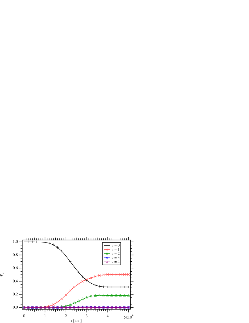
Figure 1: Projection of the time-dependent vibrational wave function of the CO molecule, interacting with a resonant laser pulse, on the first five vibrational eigenstates.

4.2 Atomic ion in a Paul trap

Let us now consider the three-dimensional problem of the motion of a charged atomic ion in a Paul trap [28, 29, 30]. These create a time-dependent quadrupolar field allowing, under the right conditions, the confinement of an ion.

The electric potential inside a Paul trap is of the form [29, 30]

$$\Phi(\mathrm{x},t)=\frac{U_{0}+V_{0}\cos\Omega t}{2d^{2}}\left(r^{2}-2z^{2}\right),$$ (26)

where $U_{0}$ is a static electric potential, $V_{0}$ the amplitude of an ac potential of frequency $\Omega$, and $r^{2}\equiv x^{2}+y^{2}$. The scale factor $d$ is obtained from $d^{2}=r_{0}^{2}+2z_{0}^{2}$, with $r_{0}$ the radial distance from the center of the trap to the ring electrode and $z_{0}$ the axial distance to an end cap (see refs. [29, 30] for more details). Considering an atomic ion of charge $Ze$, where $e$ is the elementary charge [21], we get the potential energy

$$V(\mathbf{x},t)=Ze\Phi(\mathrm{x},t).$$ (27)

For the simulation, we consider conditions similar to those of refs. [31, 32] and take a ¹³⁸Ba⁺ ion, $m=137.905232\ \mathrm{u}=2.28997005\times 10^{-25}\ \mathrm{kg}$ [33], in a trap with characteristics:

$$U_{0} =0\ \mathrm{V}$$

$$V_{0} =200\ \mathrm{V}$$

$$\Omega =2\pi\times 18\ \mathrm{MHz}$$

$$r_{0} =1.6\times 10^{-3}\ \mathrm{m}$$

$$z_{0} =r_{0}/\sqrt{2}$$

The initial state is taken as a Gaussian wave packet,

$$\psi_{\mathrm{i}}(x,y,z)=\left(\frac{2}{\pi}\right)^{3/4}\prod_{\xi=x,y,z}\frac{1}{\sqrt{\sigma_{\xi}}}\exp\left[\frac{\mathrm{i}}{\hbar}p_{\xi 0}\left(\xi-\xi_{0}\right)\right]\exp\left[-\frac{\left(\xi-\xi_{0}\right)^{2}}{\sigma_{\xi}^{2}}\right],$$ (28)

and we set

$$x_{0} =z_{0}=2\times 10^{-8}\ \mathrm{m}$$

$$y_{0} =1\times 10^{-8}\ \mathrm{m}$$

$$p_{x0} =1\times 10^{-27}\ \mathrm{kg\,m\,s}^{-1}$$

$$p_{y0} =p_{z0}=0$$

$$\sigma_{x} =\sigma_{y}=7.342\times 10^{-8}\ \mathrm{m}$$

$$\sigma_{z} =5.192\times 10^{-8}\ \mathrm{m}$$

Using $\texttt{nx}=\texttt{ny}=\texttt{nz}=512$ grid points, with the grid defined from $-1\times 10^{-6}\ \mathrm{m}$ to $1\times 10^{-6}\ \mathrm{m}$ along each Cartesian coordinate, we run the simulation for $\texttt{nt}=18\,500$ time steps of length $\Delta t=2\times 10^{-9}\ \mathrm{s}$, measuring the wave function every 10 time steps. The resulting trajectory of the ion is shown in fig. 2.

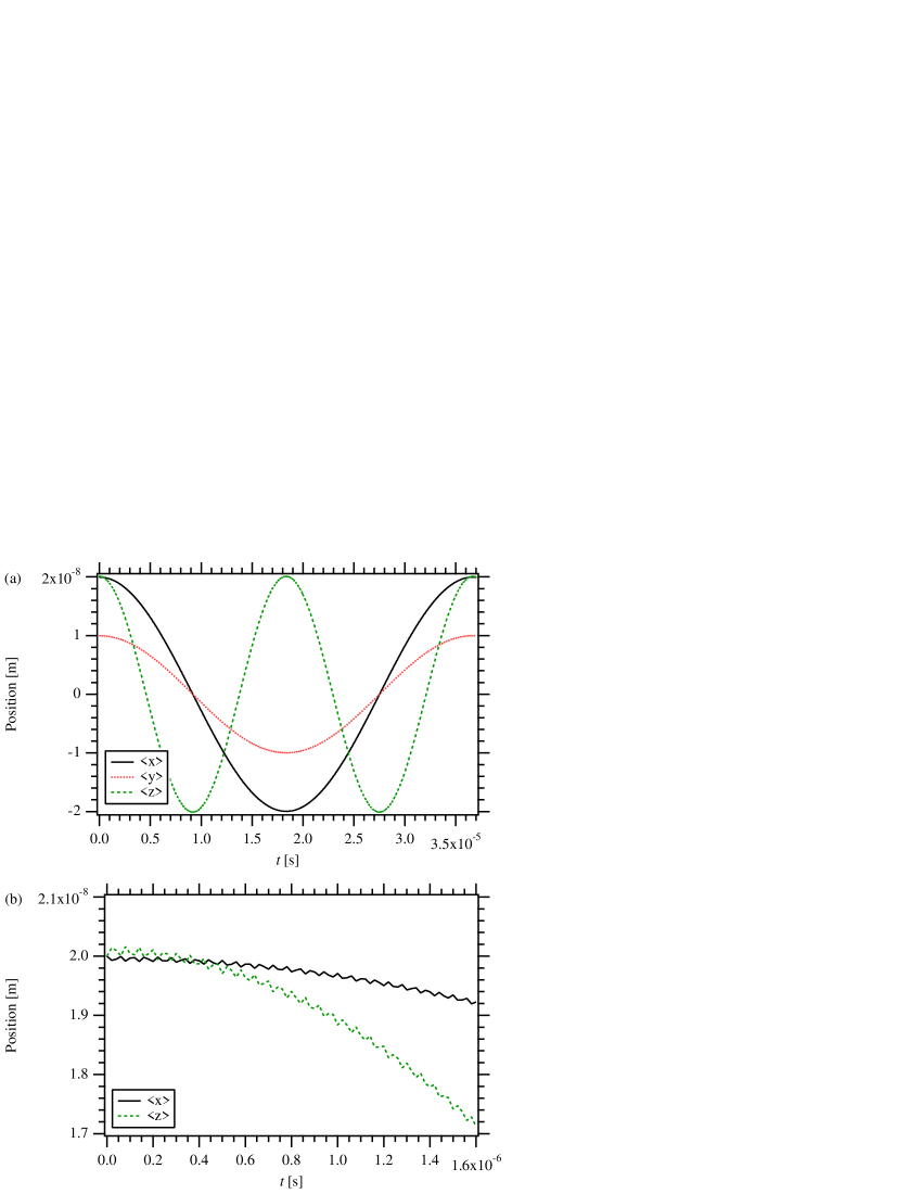
Figure 2: (a) Sample trajectory of the wave packet of a Ba⁺ ion in a Paul trap. The simulation is carried in three dimensions, and the expectation value of the position is plotted individually for each Cartesian coordinate. (b) Enlargement of panel (a), evidencing the micromotion of the ion at the frequency of the trapping potential.

References

- [1] http://gcc.gnu.org
- [2] http://www.fftw.org
- [3] http://www.mpi-forum.org
- [4] M. D. Feit, J. A. Fleck, Jr., A. Steiger, Solution of the Schrödinger equation by a spectral method, J. Comput. Phys. 47 (1982) 412–433.
- [5] M. D. Feit, J. A. Fleck, Jr., Solution of the Schrödinger equation by a spectral method II: Vibrational energy levels of triatomic molecules, J. Chem. Phys. 78 (1) (1983) 301–308.

References

- [1] V. S. Letokhov, Laser Control of Atoms and Molecules, Oxford University Press, Oxford, 2007.
- [2] M. Shapiro, P. Brumer, Principles of the Quantum Control of Molecular Processes, 2nd Edition, Wiley-VCH, New York, 2012.
- [3] J. A. Fleck Jr., J. R. Morris, M. D. Feit, Time-dependent propagation of high energy laser beams through the atmosphere, Appl. Phys. 10 (2) (1976) 129–160.
- [4] M. D. Feit, J. A. Fleck, Jr., A. Steiger, Solution of the Schrödinger equation by a spectral method, J. Comput. Phys. 47 (1982) 412–433.
- [5] M. D. Feit, J. A. Fleck, Jr., Solution of the Schrödinger equation by a spectral method II: Vibrational energy levels of triatomic molecules, J. Chem. Phys. 78 (1) (1983) 301–308.
- [6] A. D. Bandrauk, H. Shen, Improved exponential split operator method for solving the time-dependent Schrödinger equation, Chem. Phys. Lett. 176 (5) (1991) 428–432.
- [7] Y. I. Salamin, S. Hu, K. Z. Hatsagortsyan, C. H. Keitel, Relativistic high-power laser-matter interactions, Phys. Rep. 427 (2-3) (2006) 41–155.
- [8] C. M. Dion, S. Chelkowski, A. D. Bandrauk, H. Umeda, Y. Fujimura, Numerical simulation of the isomerization of HCN by two perpendicular intense IR laser pulses, J. Chem. Phys. 105 (1996) 9083–9092.
- [9] J. Javanainen, J. Ruostekoski, Symbolic calculation in development of algorithms: split-step methods for the Gross-Pitaevskii equation, J. Phys. A 39 (2006) L179–L184.
- [10] G. R. Mocken, C. H. Keitel, FFT-split-operator code for solving the Dirac equation in 2+1 dimensions, Comput. Phys. Commun. 178 (11) (2008) 868–882.
- [11] C. Cohen-Tannoudji, B. Diu, F. Laloë, Quantum Mechanics, Wiley, New York, 1992.
- [12] H.-P. Breuer, F. Petruccione, The theory of open quantum systems, Oxford University Press, Oxford, 2002.
- [13] P. Pechukas, J. C. Light, On the exponential form of time-displacement operators in quantum mechanics, J. Chem. Phys. 44 (10) (1966) 3897–3912.
- [14] S. D. Conte, C. de Boor, Elementary Numerical Analysis, 2nd Edition, McGraw-Hill, 1972.
- [15] C. Moler, C. Van Loan, Nineteen dubious ways to compute the exponential of a matrix, twenty-five years later, SIAM Rev. 45 (1) (2003) 3–49.
- [16] W. H. Press, S. A. Teukolsky, W. T. Vetterling, B. P. Flannery, Numerical Recipes in C, 2nd Edition, Cambridge University Press, Cambridge, 1992.
- [17] M. Frigo, S. G. Johnson, The design and implementation of FFTW3, Proc. IEEE 93 (2) (2005) 216–231, special issue on “Program Generation, Optimization, and Platform Adaptation”.
- [18] URL http://www.mpi-forum.org/
- [19] W. Gropp, E. Lusk, A. Skjellum, Using MPI : Portable Parallel Programming with the Message Passing Interface, MIT Press, Cambridge, MA, 1999.
- [20] URL http://www.fftw.org/
- [21] URL physics.nist.gov/constants
- [22] P. M. Morse, Diatomic molecules according to the wave mechanics. II. vibrational levels, Phys. Rev. 34 (1929) 57–64.
- [23] P. Atkins, R. Friedman, Molecular Quantum Mechanics, 5th Edition, Oxford University Press, Oxford, 2011.
- [24] K. P. Huber, G. Herzberg, Molecular Spectra and Molecular Structure: IV. Constans of Diatomic Molecules, Van Nostrand Reinhold, New York, 1979.
- [25] A. D. Bandrauk (Ed.), Molecules in Laser Fields, Dekker, New York, 1994.
- [26] J. E. Gready, G. B. Bacskay, N. S. Hush, Finite-field method calculations. IV. higher-order moments, dipole moment gradients, polarisability gradients and field-induced shifts in molecular properties: Application to N2, CO, CN-, HCN and HNC, Chem. Phys. 31 (1978) 467–483.
- [27] D. T. Colbert, W. H. Miller, A novel discrete variable representation for quantum mechanical reactive scattering via the s-matrix Kohn method, J. Chem. Phys. 96 (1992) 1982–1991.
- [28] W. Paul, Electromagnetic traps for charged and neutral particles, Rev. Mod. Phys. 62 (3) (1990) 531–540.
- [29] F. G. Major, V. N. Gheorghe, G. Werth, Charged Particle Traps: Physics and Techniques of Charged Particle Field Confinement, Springer, Berlin, 2005.
- [30] G. Werth, V. N. Gheorghe, F. G. Major, Charged Particle Traps II: Applications, Springer, Berlin, 2009.
- [31] W. Neuhauser, M. Hohenstatt, P. Toschek, H. Dehmelt, Optical-sideband cooling of visible atom cloud confined in parabolic well, Phys. Rev. Lett. 41 (1978) 233–236.
- [32] W. Neuhauser, M. Hohenstatt, P. Toschek, H. Dehmelt, Visual observation and optical cooling of electrodynamically contained ions, Appl. Phys. 17 (1978) 123–129.
-
[33]
NIST handbook of basic atomic
spectroscopic data.
URL http://www.nist.gov/pml/data/handbook/