Pre-main-sequence isochrones – II. Revising star and planet formation timescales
Abstract
We have derived ages for 13 young () star-forming regions and find they are up to a factor two older than the ages typically adopted in the literature. This result has wide-ranging implications, including that circumstellar discs survive longer () and that the average Class I lifetime is greater () than currently believed.
For each star-forming region we derived two ages from colour-magnitude diagrams. First we fitted models of the evolution between the zero-age main-sequence and terminal-age main-sequence to derive a homogeneous set of main-sequence ages, distances and reddenings with statistically meaningful uncertainties. Our second age for each star-forming region was derived by fitting pre-main-sequence stars to new semi-empirical model isochrones. For the first time (for a set of clusters younger than ) we find broad agreement between these two ages, and since these are derived from two distinct mass regimes that rely on different aspects of stellar physics, it gives us confidence in the new age scale. This agreement is largely due to our adoption of empirical colour- relations and bolometric corrections for pre-main-sequence stars cooler than .
The revised ages for the star-forming regions in our sample are – for NGC 6611 (Eagle Nebula; M 16), IC 5146 (Cocoon Nebula), NGC 6530 (Lagoon Nebula; M 8), and NGC 2244 (Rosette Nebula); for Ori, Cep OB3b, and IC 348; for Ori (Collinder 69); for NGC 2169; for NGC 2362; for NGC 7160; for Per (NGC 884); and for NGC 1960 (M 36).
keywords:
stars: evolution – stars: formation – stars: pre-main-sequence – stars: fundamental parameters – techniques: photometric – open clusters and associations: general – Hertzsprung-Russell and colour-magnitude diagrams1 Introduction
Robust and precise ages for young stars are a requirement for the advancement of our understanding of star and planet formation and evolution. These ages provide timescales with which to constrain the physical processes driving, for example, disc dissipation and planet formation (e.g. core accretion versus gravitational collapse; Pollack, 1984; Boss, 1997). Pre-main-sequence (pre-MS) ages are based on the gravitational contraction of young stellar objects (YSOs), which become increasingly faint as they contract towards the main-sequence (MS). It has been well documented that pre-MS ages are imprecise and contradictory being heavily model- (and even colour-) dependent (e.g. Naylor et al., 2002; Hartmann, 2003) with the derived ages differing by factors of up to 2 – 3 (e.g. White et al., 1999; Dahm, 2005; Hillenbrand, Bauermeister, & White, 2008).
Having highlighted the problems with the pre-MS evolutionary models, we have attempted, through a series of papers, to provide consistent pre-MS ages. In Mayne et al. (2007), pre-MS stars in a series of young star-forming regions (SFRs) were used to create a set of empirical isochrones. When plotted in absolute magnitude-intrinsic colour space these isochrones placed the clusters on a relative age ladder independent of theoretical assumptions (fiducial ages were assigned to a subset of these SFRs). The main problem with this work is that it suffered from a lack of self-consistent distance measurements, instead relying on heterogeneously derived literature estimates. To rectify this Mayne & Naylor (2008) used MS model isochrones to fit the young MS population of many of the clusters studied in Mayne et al. (2007) and derived self-consistent distances and extinctions. These revised distances, led to a subtle modification of the Mayne et al. (2007) pre-MS age scale. Although self-consistent, the Mayne et al. (2007) and Mayne & Naylor (2008) pre-MS age scale only provided relative ages. Whilst the low-mass stars in a young SFR are still on the pre-MS, the most massive objects have reached the MS, so in an effort to create an absolute age scale, Naylor (2009) used MS stars between the zero-age main-sequence (ZAMS) and terminal-age main-sequence (TAMS), in conjunction with the fitting statistic, to derive absolute ages. These MS ages were found to be a factor 1.5 – 2 times older than the pre-MS ages based on the Mayne et al. (2007) and Mayne & Naylor (2008) pre-MS age scale.
In contrast to the high level of model dependency in pre-MS evolutionary models, MS models have been shown to provide high levels of consistency (in both age and distance) between models from different groups (e.g. Mayne & Naylor, 2008; Naylor, 2009). It would seem, therefore, obvious to use MS ages, but these are imprecise compared with the pre-MS ages for two reasons. First, that the rate of change of the slope of the isochrone for a given age increment is subtle (i.e. is small, despite the precision in ). Second, in young SFRs only the most massive stars have evolved sufficiently to lie on the MS and therefore such ages are subject to large uncertainties caused by small number statistics. In terms of statistical and systematic uncertainties, pre-MS ages have small statistical but large systematic uncertainties, whereas for the MS ages the opposite is true. The approach we take in this paper, therefore, is to use the more precise pre-MS ages, but only after we have demonstrated why they differ from the MS ages, and brought them into broad agreement with the MS ages. Whilst previous studies have found either tentative evidence for agreement between the age scales for older stellar populations (; e.g. Lyra et al., 2006) or increasing disparity at younger ages (; e.g. Piskunov et al., 2004; Naylor, 2009), the recent study by Pecaut, Mamajek, & Bubar (2012) has demonstrated consistent pre-MS and MS ages for the Upper Sco subgroup of Scorpius-Centaurus based on a detailed analysis of B-, A-, F- and G-stars in the Hertzsprung-Russell (H-R) diagram.
To test whether further agreement between MS and pre-MS ages can be found for young () pre-MS clusters, we must address the main sources of uncertainty when attempting to fit pre-MS stellar populations with model isochrones. The primary issues affecting pre-MS isochrone fitting in CMDs are; i) photometric calibration of the data for what are very red stars, ii) transformation of the model isochrones from the theoretical H-R to the CMD plane, iii) incorporating the colour and gravity dependence of the interstellar extinction, and iv) the colour excesses in photometric data arising from the combined effects of stellar activity and circumstellar disc material.
The first two of these issues were explicitly addressed in Bell et al. (2012) (hereafter referred to as Paper 1). We demonstrated that the use of MS standards to transform photometric observations of young, very red pre-MS objects to a standard photometric system can introduce significant errors in the position of the pre-MS locus in CMD space. This is due to differences in the spectrum of a MS and pre-MS star of the same colour and can introduce an error of up to a factor of 2 in age for young () clusters (Bell et al., 2012). Hence, instead of the normal practice of transforming both photometric observations and theoretical models into a standard photometric system, it is crucial for precise photometric studies of pre-MS objects to leave the observations in their natural photometric system. Furthermore, Paper 1 tested several sets of pre-MS isochrones against a series of well-calibrated CMDs of the Pleiades over a contiguous wavelength range of and we showed that in optical colours no pre-MS model followed the observed Pleiades sequence at . This discrepancy was quantified in individual photometric bandpasses and showed that the model isochrones overestimated the flux by a factor of 2 at , with this difference decreasing as a function of increasing wavelength, becoming negligible at . This can also introduce an error up to a factor of 2 in age for clusters younger than (Bell et al., 2012).
The third issue to consider is the colour dependence of the interstellar reddening. Reddening estimates for a given cluster can be derived from fitting the higher mass stars with a model isochrone in the colour-colour diagram assuming a given reddening vector (that often neglects the colour and gravity dependency). This measured value is then applied to stars of all masses assuming a similar non-dependence on colour and gravity. This can inaccurately modify the shape of the pre-MS locus, especially if the target stars are highly reddened. Thus, to derive the reddening from high-mass stars in a colour-colour diagram requires a more sophisticated approach with reddening vectors that incorporate the colour and gravity dependence. To then apply this measured value to lower mass stars, the only self-consistent and homogenous method (assuming that spectra of each star are unavailable) is to create reddening and extinction grids based on atmospheric models, the appropriate system responses and a reliable representation of the interstellar extinction law. Neglecting these colour-dependent terms can introduce an error of in the derived true distance modulus (Mayne & Naylor, 2008), thereby translating into an error of per cent in the derived pre-MS age. If the extinction towards a given cluster is spatially variable, then this makes the process of deriving ages and distances more complicated. In some regions this may be due to patchy foreground extinction, but for many young SFRs () remnant gas and dust from the star formation process makes this issue more problematic still.
The final issue is which photometric bandpasses to adopt for constructing CMDs that minimise the colour excesses arising from processes including chromospheric activity, accretion, and circumstellar disc material. Accretion predominantly affects the flux shortward of the -band (Gullbring et al., 1998), whereas circumstellar disc material becomes significant for the near-infrared (near-IR) bandpasses (Lada & Adams, 1992). Lastly, Stauffer et al. (2003) showed that chromospheric activity in low-mass stars can result in an increased scatter in the and colours, whereas the colour remains unaffected. Hence, as a good compromise, we adopt the optical - and -bandpasses for this study, and investigate the pre-MS populations of our sample of SFRs using the CMD.
In this study we address, and account for, each of these issues to create a revised age scale for a sample of well-studied SFRs, and in doing so, largely remove the discrepancy between MS and pre-MS ages. In Section 2 we describe the data collection, reduction and photometric calibration, as well as the various youth diagnostics used to identify pre-MS objects. The stellar interior models, atmospheric models and the effects of reddening and extinction are discussed in Section 3, with the newly derived colour- and gravity-dependent reddening vectors explained. Section 4 describes the maximum-likelihood fitting technique, the model CMD, and the fitting of MS photometric data to derive reddenings, distances and ages. The creation of the semi-empirical pre-MS isochrones and the reddening and extinction grids are explained in Section 5. Section 6 describes the fitting of the pre-MS photometric data, with the literature sources used to identify pre-MS stars for our sample of SFRs given in Appendix A and a revised version of the maximum-likelihood fitting technique designed to deal with possible non-member contamination in the CMD discussed in Appendix B. The results from the MS and pre-MS data are brought together in Section 7 and the implications of these discussed in Section 8. Finally, our conclusions are given in Section 9. For readers interested in the final age, distance and reddening for each SFR, these results are shown in Table 8 in Section 7.1.
2 The Data
The observations presented were obtained using the 2.5-m Isaac Newton Telescope (INT) on La Palma at the same time as our Pleiades observations described in Paper 1. We refer the reader to Paper 1 for details of our observational techniques, photometric calibration, and data reduction. As in Paper 1, the astrometric calibration was provided using objects in the Two-Micron All-Sky Survey (2MASS, Cutri et al., 2003), with a rms of approximately for the fit of pixel positions as a function of RA and Dec.
It is important for what follows that our final catalogues are in the natural photometric system of the Wide-Field Camera (WFC) on the INT (hereafter INT-WFC) calibrated to the absolute AB photometric system (Oke & Gunn, 1983). In Paper 1 we adopted a clipping radius of the full-width at half maximum (FWHM) of the seeing, however, in these more crowded fields this was reduced to (for a full discussion see King et al. in preparation). Table 1 shows the central coordinates for each field-of-view and limiting magnitude in the INT-WFC bandpasses for our sample of SFRs.
| SFR | (J2000.0) | (J2000.0) | Limiting magnitude in bandpasses |
|---|---|---|---|
| Cep OB3b | 21.4, 23.4, 23.5, 23.2, 22.3 | ||
| Per | 21.4, 22.9, 22.9, 22.7, 21.9 | ||
| IC 348(1) | – , 22.0, 22.0, 22.1, 21.4 | ||
| IC 5146 | 21.4, 22.8, 22.9, 22.5, 21.6 | ||
| Ori A | 20.5, 22.6, 22.6, 22.6, 21.7 | ||
| Ori B | 20.6, 22.6, 22.5, 22.4, 21.6 | ||
| Ori C | 20.6, 22.8, 22.6, 22.6, 21.7 | ||
| Ori D | 20.8, 22.9, 22.6, 22.9, 21.9 | ||
| NGC 1960 | 19.0, 22.8, 22.8, 22.6, 21.8 | ||
| NGC 2169 | 21.7, 22.9, 22.8, 22.5, 21.8 | ||
| NGC 2244 | 21.4, 22.8, 22.7, 22.4, 21.5 | ||
| NGC 2362 | 21.2, 22.7, 22.5, 22.1, 21.2 | ||
| NGC 6530 | 20.3, 21.5, 21.5, 21.5, 20.8 | ||
| NGC 6611 | 20.5, 23.0, 22.4, 21.9, 21.0 | ||
| NGC 7160 | 19.0, 22.2, 22.3, 22.6, 22.0 | ||
| Ori A | 19.5, 22.8, 22.8, 22.6, 21.5 | ||
| Ori B(2) | – , 23.0, 22.8, 22.8, 21.6 | ||
| Ori C | 18.3, 22.8, 22.8, 22.5, 21.6 | ||
| Ori D(1) | – , 22.9, 22.7, 22.6, 21.4 |
For the field-of-view centred on IC 348, in all but the central CCD there were too few stars to create the profile correction necessary to correct the optimal photometry. Hence for stars in these regions aperture photometry was performed with the radius of the aperture matching that used in the case of the profile correction (15 pixels). The resultant fluxes were then processed in an identical manner to that in the standard reduction. The only difference is that the non-stellar flag ‘N’ (see Burningham et al., 2003) is now based on the ratio of the flux measured through an aperture of 7 pixels. To create the final optical photometric catalogue, all stars flagged ‘H’ (poor profile correction) in the optimally extracted catalogue were replaced with measurements based on the aperture photometric reduction.
For Cep OB3b, Per, IC 5146, and Ori A observations were taken on two separate nights for which there is a photometric solution. The two sets of observations were reduced separately and a normalisation procedure performed on the two optical photometric catalogues, so that the zero-point is the average of the two nights. As discussed in Naylor et al. (2002), the calculated zero-point shift is a good indicator of the internal consistency of the photometry, as well as the accuracy with which the profile corrections were performed. For regions where the normalisation procedure was used an accuracy of 2 – 3 per cent was found across all colours.
| SFR | Table number | Description | Source |
|---|---|---|---|
| Cep OB3b | 9 | Full catalogue | |
| 10 | Members | 1+2 (X-ray); 3 (Spectroscopic); 4 (H); 5 (Periodic variable) | |
| Per | 11 | Full catalogue | |
| 12 | Positionally isolated | ||
| IC 348 | 13 | Full catalogue | |
| 14 | Members | 6 (H); 7+8+9 (Spectroscopic); 10+11 (X-ray); 12+13 (Periodic variable) | |
| IC 5146 | 15 | Full catalogue | |
| 16 | Members | 14 (H); 15 (IR excess) | |
| Ori | 17 | Full catalogue | |
| 18 | Members | 16+17+18 (Spectroscopic); 19 (IR-excess); 20 (X-ray) | |
| NGC 1960 | 19 | Full catalogue | |
| 20 | Members | 21 (Spectroscopic) | |
| NGC 2169 | 21 | Full catalogue | |
| 22 | Members | 22 (Spectroscopic) | |
| NGC 2244 | 23 | Full catalogue | |
| 24 | Members | 23 (X-ray); 24 (IR excess) | |
| NGC 2362 | 25 | Full catalogue | |
| 26 | Members | 25 (Spectroscopic); 26 (IR excess); 27 (X-ray) | |
| NGC 6530 | 27 | Full catalogue | |
| 28 | Members | 28 (X-ray); 29 (Spectroscopic); 30 (Periodic variable) | |
| NGC 6611 | 29 | Full catalogue | |
| 30 | Members | 31 (X-ray); 32 (IR excess) | |
| NGC 7160 | 31 | Full catalogue | |
| 32 | Members | 33 (Spectroscopic and extinction); 34 (IR excess) | |
| Ori | 33 | Full catalogue | |
| 34 | Members | 35+36+37 (Spectroscopic); 38 (X-ray); 39 (Periodic variable) |
For the identification of pre-MS members we have used literature sources that use specific youth indicators to discriminate between them and older field stars. Appendix A discusses the adopted literature sources for each SFR, a summary of which is presented in Table 2. For each SFR we have typically used a range of membership criteria (e.g. X-ray, spectroscopic features, periodic variability, and IR excess) and these will each have an associated inherent bias.
To derive consistent pre-MS ages from CMDs of such populations it is vital that these biases be understood, and if possible minimised. In brief, IR excesses predominantly identify objects with circumstellar discs, X-rays are more likely to select stars that are not actively accreting, H is biased towards stars that are actively accreting, and periodic variability preferentially selects weak-lined T-Tauri stars (although classical T-Tauri stars can be identified if the temporal density of observations is sufficiently high; e.g. Littlefair et al., 2005). Members that have been selected via non-spectroscopic methods are more likely to suffer from foreground and background contamination. Spectroscopic indicators are probably the only unbiased diagnostic, however herein lies a subtle bias which can be introduced through a pre-selection of candidate targets. Full spectroscopic coverage of all stars in a given field-of-view is unfeasible and so a subset of stars is chosen, generally based on their position in CMD space. This therefore introduces an inherent bias into the observed subset of stars, however as demonstrated by the studies of Kenyon et al. (2005) and Burningham et al. (2005), even adopting a relatively conservative photometric selection does not exclude a statistically significant number of members, and hence the observed pre-MS locus is largely unbiased by such pre-selection.
All of the catalogues presented in this study are freely available from the Cluster Collaboration home page111http://www.astro.ex.ac.uk/people/timn/Catalogues/ and the CDS archive. Table 2 shows the full list of photometric catalogues, with a sample of the full photometric catalogue for Ori shown in Table 3. Figs. 8 – 16 showing CMDs in the INT-WFC photometric system, as well as the members catalogues (see Table 2), use data where stars variable from night-to-night have been replaced by the values from one night as described in Paper 1. For the data plotted in Figs. 8 – 16 we retain only those objects with uncertainties in both colour and magnitude of , however the full photometric catalogues include all identified sources.
| Field | ID | R.A. (J2000.0) | Dec. (J2000.0) | x | y | Flag | Flag | ||||
|---|---|---|---|---|---|---|---|---|---|---|---|
| 50.02 | 4 | 05 35 12.784 | +09 36 47.51 | 973.790 | 1426.059 | 8.148 | 0.010 | OS | 0.309 | 0.014 | SS |
| 54.03 | 70 | 05 35 13.200 | +10 14 24.79 | 991.198 | 929.162 | 8.221 | 0.010 | OS | 0.205 | 0.014 | SS |
2.1 Main-sequence literature data
| SFR | Source |
|---|---|
| Cep OB3b | Blaauw, Hiltner, & Johnson (1959) |
| Per | Johnson & Morgan (1955) |
| IC 348 | Harris, Morgan, & Roman (1954) |
| IC 5146 | Walker (1959) |
| Ori | Murdin & Penston (1977) |
| NGC 1960 | Johnson & Morgan (1953) |
| NGC 2169 | Hoag et al. (1961) |
| NGC 2244 | Johnson (1962) |
| NGC 2362 | Johnson & Morgan (1953) |
| NGC 6530 | Walker (1957) |
| NGC 6611 | Walker (1961) |
| NGC 7160 | Hoag et al. (1961) |
| Ori | Hardie, Heiser, & Tolbert (1964) |
| Greenstein & Wallerstein (1958); Guetter (1979) |
As the WFC saturates at magnitudes we were required to include literature data so that we could derive ages, distances and reddenings from the MS populations. To determine statistically meaningful parameters from these objects we require a significant mass range to; i) display measurable evolution between the ZAMS and TAMS and ii) derive robust reddening and distance measurements which can then be applied to the low-mass regime when fitting the pre-MS data. photometry provides us with the necessary information to derive all of these quantities. Reddenings can be calculated from fitting data in the colour-colour diagram and distances can be derived through the traditional MS fitting technique, utilising stars that have yet to turn off the ZAMS and begin their evolution towards the TAMS. Additionally, the upper region of the CMD is age sensitive, tracing out the evolution between the ZAMS and TAMS. Table 4 details the literature sources for the MS photometry for our sample of SFRs.
To maintain consistency within our photometric data, we used, whenever possible, the photoelectric photometry of Johnson and collaborators. These pioneering works defined and characterised the photometric system, and provide us with the levels of calibration and consistency required. Note that robust uncertainties are cited in many of the sources, however as the uncertainty in colour is always smaller than for the observed magnitude, we therefore treat the uncertainties as uncorrelated.
3 The Models
To derive parameters, such as age and distance, from fitting photometric data in CMDs we require model isochrones, which must be calibrated to the same photometric system as that of the data. Model isochrones are generated using stellar interior models that predict the bolometric luminosity (), effective temperature () and surface gravity (log) for a given mass. These quantities are then transformed into colours and magnitudes to compare to measured values. Colours are calculated using a colour- relation and magnitudes via bolometric corrections (BCs) to . Both relations can be derived by folding atmospheric models through the appropriate photometric filter responses and we describe the details of doing so in Appendix B of Paper 1. Here we describe our choice of interior and atmospheric models.
3.1 Pre-main-sequence models
The pre-MS interior models used in this study are the same as those adopted in Paper 1, namely those of Baraffe et al. (1998) with a solar-calibrated mixing-length parameter , D’Antona & Mazzitelli (1997) and Dotter et al. (2008) models (hereafter BCAH98 , DAM97 and DCJ08 respectively). Note that the interior models of Baraffe et al. (1998) with a general mixing-length parameter and Siess, Dufour, & Forestini (2000) are not used in this analysis as both models systematically overestimate stellar luminosities for masses and fail to match the observed Pleiades MS (see Paper 1).
3.2 Main-sequence models
We adopted the Geneva interior models of Lejeune & Schaerer (2001), specifically the basic ‘c’ grid (Schaller et al., 1992). The rate of change of and with time changes discontinuously at the TAMS, and as the grid of interior models is much coarser than that required, intermediate age models were created by temporally interpolating between existing calculations. For this an interpolation routine provided by the Geneva group was used to create a grid with spacing .
It should be noted that the Schaller et al. (1992) MS models do not consider the pre-MS evolutionary phase, but only that from the ZAMS onwards. The ages derived for our sample of SFRs are driven by the most massive stars i.e. those that have evolved significantly from the ZAMS, which, as the SFR ages, decrease in mass. For our oldest SFR (NGC 1960) the age is based on stars with spectral types of BII–III (see Johnson & Morgan, 1953), which, from the evolutionary models of Siess et al. (2000), have masses of and take to arrive on the ZAMS. Hence, although the Schaller et al. (1992) models do not include pre-MS evolution, the timescales involved are significantly shorter than the uncertainties on the derived ages themselves and therefore can be safely neglected.
3.3 Atmospheric models
The atmospheric models used are the same as those in Paper 1 and consist of phoenix BT-Settl models (Allard, Homeier, & Freytag, 2011)222http://phoenix.ens-lyon.fr/Grids/BT-Settl/ for and the Kurucz atlas9/ODFnew models (Castelli & Kurucz, 2004)333ftp://ftp.stsci.edu/cdbs/grid/ck04models for . Despite differences in the underlying physical assumptions and adopted parameters, we found that at the transitional all derived colours from both sets of models agreed to within .
To transform the MS interior models into the Johnson photometric system, we derived BCs using Eqn. B2 of Paper 1 and the standard responses of Bessell (1990b). To account for the fact that the photoelectric system is based on an energy integration method, Eqn. B2 of Paper 1 was modified so that the factor of in the integrands on the third term were removed, such that,
where is the total flux emergent at the stellar surface and all other symbols retain their original definitions (see Paper 1). For the solar values we used and (Bessell, Castelli, & Plez, 1998). To define and we required a Vega reference spectrum and for this we used the CALSPEC alpha_lyr_stis_005444http://www.stsci.edu/hst/observatory/cdbs/calspec.html spectrum with and all colours equal to zero. We hereafter refer to the transformed MS isochrones as the Geneva-Bessell isochrones.
In the MS interior models, some of the most luminous stars have associated log values that lie just below the range provided by the atmospheric models. In such cases, it was necessary to extrapolate the models by setting the colour equal to that of the nearest log. As the log dependence is very small at such , this extrapolation affects the model isochrone at level.
Note that the commonly referred to colour- relation can also be represented simply in terms of BCs as it is the difference in the BCs at a specific that explicitly defines the colour of the star i.e.
and so from now on the transformation from H-R to CMD space will be discussed in terms of the BC- relation.
3.4 Reddening vectors in the Bessell system
In broadband photometry, the effective wavelength of a given bandpass moves depending on the incident stellar flux distribution, and hence the colour (and gravity) of the star (see Bessell et al., 1998). This variation results in a non-linear reddening vector in the colour-colour diagram, which further depends, albeit to a lesser extent, on the intrinsic reddening of the observed source (Hiltner & Johnson, 1956; Wildey, 1963).
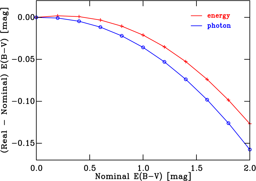
Whilst canonical linear reddening laws (such as the standard ; Johnson & Morgan, 1953) can be used to de-redden stars photometrically, our derived age is heavily dependent upon the subtle evolution between the ZAMS and TAMS, and therefore, for the level of precision required in this study it is important to understand how stars of varying colour move as a function of reddening in the colour-colour diagram. We can quantitatively model these reddening vectors by reddening the atmospheric models according to the parameterised extinction law of Cardelli, Clayton, & Mathis (1989) and folding them through the standard responses of Bessell (1990b). Note that we only use atmospheric models with intrinsic colours to derive the reddening vectors. The parameterised extinction law can be visualised in terms of a nominal (hereafter ) which represents the amount of intervening interstellar material between an observer and the object, but does not necessarily correspond precisely to the observationally measured value since this value will vary with the colour of the star.
To determine the relationship between the nominal and measured values we reddened the atmospheric models using the Cardelli et al. (1989) extinction law in steps of 0.2 from . For the value of the total-to-selective extinction ratio we adopted as an appropriate value for the diffuse interstellar medium (ISM). Measured values were inferred from the reddened atmospheric models at an intrinsic colour . Fig. 1 shows the difference between the nominal and measured as a function of and highlights the non-linear relation between the two quantities.
As discussed in Bessell (1990b), the Johnson colour is best reproduced through the use of the standard and bandpasses, however, the colour is best represented using the modified and responses (which account for increased atmospheric absorption; see Bessell, 1990b). Therefore, for both the calculated colours and reddening vectors we have used the and responses for the colour. The reddening vectors are,
and
where the dependence on both the colour of the star and the intrinsic reddening of the source are explicitly incorporated. These reddening vectors are accurate to within , however this degrades to at the limiting .
The value of is typically assumed to be a function of the line-of-sight towards a given object. Whereas in most cases it is appropriate to assume that , there is substantial evidence that this is not always the case and that for very young SFRs the reddening law may be significantly different. The effect of this on our results is discussed further in Section 4.2.3 for our sample of SFRs.
4 Fitting the young main-sequence
We used the fitting statistic555The fitting statistic software and implementation details are available at http://www.astro.ex.ac.uk/timn/tau-squared of Naylor & Jeffries (2006) and Naylor (2009) to derive ages, distances and reddenings from the MS populations of our sample of SFRs. The fitting statistic can be viewed as a generalisation of the statistic where both the model isochrone and the data are two-dimensional distributions (uncertainties in both colour and magnitude for the photometric data and a widening of the isochrone due to an intrinsic binary fraction). The best-fit model is found by minimising . We used the Geneva-Bessell models to fit the MS stars, with reddenings calculated using the colour-colour diagram, and ages and distances derived simultaneously using the CMD.
The shaded region in Fig. 2, and all subsequent figures showing photometric data fitted using , represents the two-dimensional model distribution. In this context, the model distributions are probability density distributions (the term in Eqn. 1 of Naylor & Jeffries, 2006) in CMD space obtained by applying binarity to a model isochrone at a given age. In all figures showing fitted data, for which a mean reddening was derived (see Section 4.2.1), the models have been adjusted to apparent colour-magnitude space using the measured and the reddening vector given in Section 3.4. For regions where the reddening was found to be spatially variable (see Section 4.2.2) the age and distance were calculated by fitting the photometric data in the de-reddened intrinsic colour-magnitude space.
4.1 The model CMD
We first created the probability distribution function to fit to the photometric data. The model CMD is created using a Monte Carlo method to simulate stars over a given mass range. An important part of our fitting method is that we include binaries, though as shown in Naylor & Jeffries (2006) for low-mass stars and Naylor & Mayne (2010) for high-mass stars the precise form of the mass-ratio distribution and binary fraction used is not crucial. For masses of and greater we followed the formalism of Naylor & Mayne (2010) and assumed an O-star binary fraction of 75 per cent. Of these, 25 percent are evenly distributed over , 75 per cent are evenly distributed over , and a lower restriction of is adopted. For masses below we adopted a binary fraction of 50 per cent and a uniform secondary distribution ranging from zero to the mass of the primary.
The mass function adopted does not have a significant impact on the best-fitting parameters (see (Naylor, 2009)), and so for each star a mass is drawn from a power law distribution () which results in a roughly even distribution of stars as a function of magnitude. If the star happens to be a binary the companion mass is assigned as described above. The interior model then assigns an , and log which can be converted into CMD space using the appropriate BC- relation. Binary companions that lie below the lower mass limit of the interior models are assumed to have a flux equal to zero and thus provide no contribution to the overall luminosity of the binary system.
4.2 Extinction fitting
Having established the importance of the reddening (see Section 3.4) we must first derive this, as changing this value will subsequently modify the age and distance derived by fitting the CMD. For this, we followed the two-step method as described in Mayne & Naylor (2008).
4.2.1 Uniform reddening
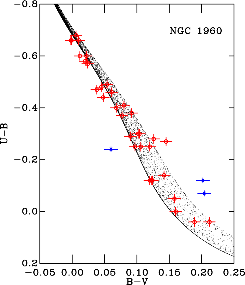
For each SFR a mean reddening was determined by fitting a model isochrone (which included an intrinsic binary fraction) using the reddening vector given in Eqn. 3.4. We used to find the best fitting extinction. An example of such a fit is shown in Fig. 2 for NGC 1960. Only stars defined as members by Johnson & Morgan (1953) and those bluewards of were used. We further removed three additional stars (Boden 50, 86 and 110) due to a combination of their positions in the colour-colour diagram and high values (see Fig. 2). For the remaining stars the best-fitting was 0.20.
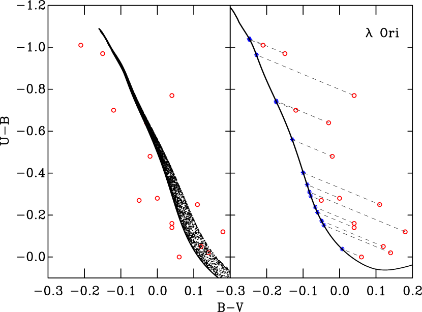
A second, less successful example of fitting the colour-colour diagram assuming a uniform reddening is shown in the left panel of Fig. 3 for the Ori association. Only stars identified as members by Murdin & Penston (1977) have been used. The best-fiting is 0.14, but as is clear from Fig. 3 the data show an unacceptable scatter about the fitted sequence. This conclusion is supported by the associated which is (as compared to 0.2 for NGC 1960). is exactly analogous to , giving the probability that a dataset resulting from observing a SFR whose parameters were those of the best-fit, would yield a value of which was greater than that actually obtained. In this case it is indicating that the model is an unacceptable fit to the data, implying the reddening is spatially variable across the Ori association.
Our adopted procedure, therefore, is to fit the data for all the SFRs with a uniform extinction model. If the best fitting extinction is adopted. In all such cases the uncertainties in were less than , and so are negligible in our analysis. If the fit is poor (i.e. ), we de-redden the stars individually using the method described below (see also the right panel of Fig. 3).
4.2.2 Variable reddening
To determine individual stellar reddenings we have used a revised Q-method. The Q-method is used to photometrically de-redden stars individually using the colour-colour diagram. Whilst we carry out this process numerically, Johnson & Morgan (1953) parameterised the intersection of a linear MS and linear reddening vectors to create an extinction independent colour, Q. As noted in Mayne & Naylor (2008), this can result in errors in the extinction of up to due to assuming a linear MS with an additional error of through the use of colour independent reddening vectors. We therefore fitted a straight line to the Geneva-Bessell model isochrone and incorporated the colour- and extinction-dependent reddening vector shown in Eqn. 3.4 to give
By replacing the original Q-method MS straight line with a line fitted to a section of the Geneva-Bessell model isochrone, it is necessary to assume a given age. Unlike the evolution of the MS in the CMD, the MS in the colour-colour diagram moves very little with age (see Mayne & Naylor, 2008). As a given sequence ages, stars of increasingly lower mass evolve away from the MS. Hence when using the revised Q-method to de-redden stars individually, it is important to ensure that any post-MS objects are not included as these will be incorrectly de-reddened and therefore occupy the wrong position in both the colour-colour and CMD.
Where possible, it is better to fit for a mean reddening using the technique. The revised Q-method implicitly assumes that all stars are either single-stars or equal-mass binaries and is thus unable to account for the scatter in CMD space as a result of binarity and photometric uncertainties. The effects of binarity are non-negligible. Although in colour-colour space the single-star and equal-mass binary sequences are co-incident, not knowing whether the star should lie on that sequence or somewhere in the unequal-mass binary region (see the unequal-mass binary distribution in Fig. 3) can affect the derived extinction on the level (Mayne & Naylor, 2008). This effect becomes more marked as one moves towards lower masses (redder colours) along the MS model isochrone.
4.2.3 Anomalous line-of-sight extinction
There have been numerous suggestions in the literature that the reddening law towards very young SFRs may differ from that characteristic of the normal ISM. Such anomalous reddenings may be caused by photoevaporation of small dust grains by nearby massive stars or grain growth in circumstellar environments (Cardelli & Clayton, 1988; van den Ancker et al., 1997), resulting in large values for the total-to-selective extinction ratio . It has been shown explicitly that there is an anomalous reddening law towards NGC 6611 (e.g. Hiltner & Morgan, 1969; Hillenbrand et al., 1993). Polarimetric observations by Orsatti, Vega, & Marraco (2000, 2006) have shown that the size of silicate and graphite dust grains in NGC 6611 might be larger than those in the typical ISM. Values of range from , with a typical value of (Hillenbrand et al., 1993).
We have therefore recalculated the reddening vectors (Eqns. 3.4 and 3.4) adopting this typical value of , and derived the MS age, distance and reddening for NGC 6611 under this assumption (see Table 5). Note, however, that due to possible variations in in NGC 6611 the distance derived in Section 4.3 based on MS fitting may (in the most extreme cases) be up to larger or smaller. The effects of this uncertainty in the derived distance are further discussed in Section 7.2.
4.3 Age and distance fitting
With a calculated mean reddening for a given SFR the next step is to redden the model isochrones so that they can be used to fit the data in the plane for distance and age. We used the calculated reddening vector shown in Eqn. 3.4 to create model isochrones at the appropriate reddening. For SFRs that showed variable reddening, and were hence de-reddened using the revised Q-method, the model isochrones were left in intrinsic space.
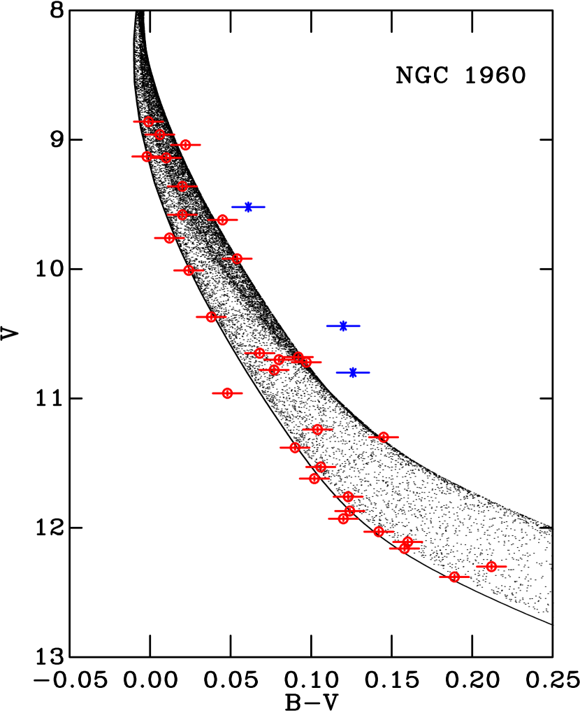
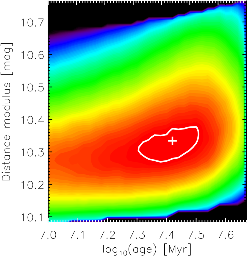
An example of fitting the CMD for age and distance simultaneously is shown in Fig. 4 for NGC 1960. After fitting for , we removed three stars (Boden 13, 47 and 48) based on a combination of their positions in the CMD and their associated values (see Fig. 4). We fitted the remaining stars and calculated an age of and a distance modulus with . Fig. 5 shows the corresponding age-distance grid for NGC 1960. The large cross defines the lowest within the grid and therefore the best-fitting values. The contour is at the 68 per cent level and defines the uncertainties in the derived age and distance. The best-fitting CMDs for the remainder of our sample of SFRs are shown in Fig. 6
| SFR | MS Age (Myr) | Distance modulus | ||||
|---|---|---|---|---|---|---|
| Best-fit | 68 per cent | Best-fit | 68 per cent | |||
| NGC 6611(1,2) | 4.6 | 3.9–6.0 | 11.38 | 11.08–11.44 | 0.17 | 0.71 (0.58) |
| Cep OB3b(1) | 6.0 | 3.8–6.6 | 8.78 | 8.70–8.84 | 0.26 | 0.89 (0.41) |
| NGC 6530(1) | 6.3 | 5.7–7.0 | 10.64 | 10.59–10.68 | 0.98 | 0.32 (0.23) |
| NGC 2244(1) | 6.6 | 5.8–7.4 | 10.70 | 10.67–10.75 | 0.70 | 0.43 (0.18) |
| Ori(1) | 8.7 | 4.7–13.4 | 8.05 | 7.99–8.11 | 0.16 | 0.05 (0.12) |
| Ori(1) | 10.0 | 8.9–11.0 | 8.02 | 7.99–8.06 | 0.49 | 0.11 (0.24) |
| NGC 2169 | 12.6 | 10.5–17.6 | 9.99 | 9.90–10.06 | 0.20 | 0.16 |
| NGC 2362 | 12.6 | 7.9–15.3 | 10.60 | 10.57–10.66 | 0.31 | 0.07 |
| NGC 7160(1) | 12.6 | 10.5–13.9 | 9.67 | 9.62–9.76 | 0.29 | 0.37 (0.37) |
| Per(1) | 14.5 | 12.8–16.7 | 11.80 | 11.77–11.86 | 0.49 | 0.52 (0.28) |
| NGC 1960 | 26.3 | 21.1–29.5 | 10.33 | 10.28–10.35 | 0.67 | 0.20 |
| IC 348(1,3) | – | – | 6.98 | 6.89–7.17 | – | 0.69 (0.52) |
| IC 5146(1,3) | – | – | 9.81 | 9.62–10.01 | – | 0.75 (0.61) |
The MS populations of both IC 348 and IC 5146 lack a sufficient number of evolved stars to constrain a MS age. Individual stars were de-reddened using a combination of the revised Q-method and spectral types to determine the best-fit solution. A photometric parallax distance for both SFRs was calculated in an identical manner to the fitting routine used for the other SFRs in our sample.
The ages, distances and reddenings for all SFRs derived using the Geneva-Bessell model isochrones are shown in Table 5. For SFRs where the reddening appears uniform, we show only the mean , whereas for SFRs with variable reddening we note the median and the full range in for all MS members in parentheses.
4.4 Discussion
In this section a self-consistent set of MS ages, distances and reddenings have been derived for a sample of young () SFRs to, in most cases, a higher level of precision than that existing in the literature, with statistically meaningful uncertainties in the derived ages and distances. It is instructive to place these new derivations in context by comparing them with previous determinations for these regions. Seven of the SFRs studied here have also been investigated by Naylor (2009). Comparing these results, the most obvious conclusions that can be drawn are; i) the best-fit MS ages presented in this study are, in all but one case, older than those in Naylor, ii) the distances derived here are consistent with those of Naylor, and iii) the associated values in this study are, in general, higher than those of Naylor, indicating that the models adopted in this study represent a better fit to the photometric data.
The older ages derived in this study are primarily due to adopting different atmospheric models to those of Naylor (2009), and to a lesser extent, to the use of colour- and extinction-dependent reddening vectors. The difference is most significant in the -band which affects the position of de-reddened stars and therefore the age required to best-fit the photometric data. Given that both the interior models and the photometric datasets used in this study and that of Naylor are the same, the fact that the associated values for the MS distance-age fits are higher in this study suggests that the revised model atmospheres provide a better fit to the data and consequently that the use of the updated atmospheric models is correct. Furthermore, it suggests that the conversion from H-R to CMD space derived in Section 3.3 represents an improved description of the Johnson photometric system compared to that of Bessell et al. (1998). Finally, it implies that the MS parameters derived in Section 4.3 are more robust than those of Naylor (2009).
5 Semi-empirical pre-main-sequence isochrones
As discussed in Section 3, BC- relations can be derived by folding the flux distribution from model atmospheres through the filter responses for the appropriate photometric system. However, it is well known that such a procedure overestimates the optical flux for stars cooler than , a result we quantified in Paper 1. This is thought to be because the model atmospheres have an incomplete description of the opacity in the optical. Given that the differences between the theoretical and empirical BCs can be as much as , corresponding to a factor 2 difference in age, it is clear we must use empirical BCs for lower than .
The usual source for empirical BCs has been observations of MS stars (e.g. Johnson, 1966; Schmidt-Kaler, 1982; Bessell, 1990a; Flower, 1996). The problem with such an approach for pre-MS fitting is that empirical BCs do not have any allowance for the difference in log between MS and pre-MS stars. According to the BCAH98 models the log of a star increases by almost between and reaching the ZAMS. This makes a difference of order to the BC in the -band predicted by the BT-Settl atmospheric models. Hence the difference in log is marginally significant (20 per cent in age), but equally importantly, if we fail to make some adjustment for log, there will be a discontinuity in our model isochrones at the point that we switch from theoretical to empirical BCs, and the size of that discontinuity will be age dependent.
Rather than using MS stars with their mix of metallicities, we follow Stauffer et al. (1998) and Jeffries, Thurston, & Hambly (2001) and use the Pleiades, whose metallicity is, to within the uncertainties, solar. We derive the empirical BC at each point along the Pleiades sequence of Bell et al. (2012), and then express this as a correction to the theoretical BC derived for the appropriate and log for that point in the sequence. As shown in Paper 1, the models fit the -band flux well, and so we chose this to fix the at each point in the sequence666Unlike other versions of this technique, this leaves us with a well defined mass scale for the younger clusters, tied to the Pleiades.. The result is a set of -dependent corrections to the BCs. We then return to the theoretical BC grid in and log and add the appropriate correction for the to each entry, irrespective of its log. This yields a set of log-dependent semi-empirical BCs. Note, that as demonstrated in Paper 1, we only apply corrections to the theoretical BC- relation up to as at higher the model isochrones match the observed shape of the Pleiades sequence.
The assumption of log independence in the correction to the BC is equivalent to assuming that the missing opacity has the same log dependence as the remaining opacity. Whilst such an assumption is far from unassailable, as the models give a difference in BC for the appropriate change in gravity of only , we need only a very crude log correction to push its effects below the level at which they matter. Furthermore, the assumption is tested by our fitting, where at least for stars older than we obtain good fits to the data (see Section 6).
5.1 Reddening and extinction for pre-main-sequence stars
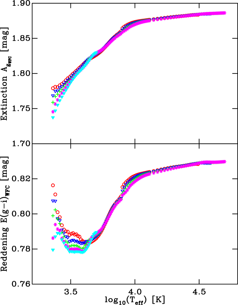
Fig. 7 shows how the calculated extinction and reddening, in the -band and colour respectively, vary as a function of for stars with for a . For hot stars () there is little variation, thus one can reliably model reddening vectors for stars in this regime that apply over a large (or equivalently spectral type) range. The same, however, is not true for cool stars where a difference in the extinction of and reddening of is calculated between stars with and . This not only demonstrates that applying the extinction and reddening derived from high-mass stars in a given SFR to those in the low-mass regime is incorrect, but furthermore that the same reddening vectors should not be used for all spectral types.
Without spectra for a large sample of objects in a given field-of-view, it is not possible to de-redden sources on an individual basis and then fit the model isochrones in the extinction-corrected CMD. Instead, the isochrone must be appropriately reddened and then applied to the photometric data. The only consistent and homogeneous way to redden the pre-MS model isochrones, as a function of , is to create extinction grids based on atmospheric models, the photometric system responses, and a description of the interstellar extinction law. The atmospheric models were reddened according to the parameterised extinction law of Cardelli et al. (1989) and folded through the calculated INT-WFC system responses (see Paper 1). The models were reddened in steps of 0.5 from , with the grids comprising extinction in all INT-WFC bandpasses as a function of and log (both of which come from the atmospheric models). Thus to redden a pre-MS model isochrone, the reddening derived from the more massive MS members is used to calculate a that represents the column density of interstellar material between the Earth and the star. This is then used to interpolate within the extinction grids for the extinction and reddening (difference in extinction between two bandpasses) for a star of given and log as defined by the pre-MS interior models. This process is then repeated for each point along the model isochrone.
6 Fitting the pre-main-sequence
Conceptually, there is no difference between fitting the pre-MS and MS populations of a given SFR using the fitting statistic. There are a couple of examples in the literature (e.g. Naylor & Jeffries, 2006; Cargile & James, 2010) where has been used to derive pre-MS ages by fitting the positions of probable low-mass members using model distributions (isochrones including an intrinsic binary fraction; see Section 4.1). In these examples, the clusters represent relatively old pre-MS populations () in which the pre-MS locus is well defined, and as such the age and distance were fitted simultaneously. These studies showed that the main contributor to the error budget in the age were uncertainties in the derived distance. This is unsurprising given the degeneracy between derived age and assumed distance when fitting pre-MS model isochrones to photometric data in CMDs.
As one moves to slightly younger populations (), the pre-MS locus, though still well-defined in CMD space, begins to exhibit an enhanced luminosity spread at a given colour, perhaps as a result of astrophysical processes in the form of, for example, enhanced variability arising from the inclusion of accreting objects in samples. This spread can, however, be exaggerated by the inclusion of non-members in the sample. Spectroscopic measurements are the only unbiased diagnostic, although, in many cases other diagnostics (e.g. X-ray emission, IR excess or H emission) have been used to differentiate between young SFR members and older field stars. As a result, these methods are more likely to include contamination from foreground and background objects than memberships based on purely spectroscopic methods. One way of ensuring that such non-members do not influence the derived age is to adopt a so-called soft-clipping approach, whereby data points with colours and magnitudes that lie several away from the observed sequence are assigned an arbitrary low probability as they are not well described by the model distribution (e.g. Naylor & Jeffries, 2006). In Appendix B a model dealing with such interlopers by modelling a background population of non-member stars in conjunction with the bona fide cluster members is introduced. The assumption of a uniform distribution of non-members is a poor description of the physical distribution, but as shown in Appendix B it does allow the correct best-fitting age to be derived, although it will result in incorrect uncertainties in that age. Practically, however, our uncertainty in the derived age is driven by the uncertainty in the distance from our MS fitting and so we derive the uncertainty in age by fitting at the two extremes of the distance estimate. In Section 6.1 this model is thus implemented and the fitting statistic is used to derive pre-MS ages for SFRs with MS ages .
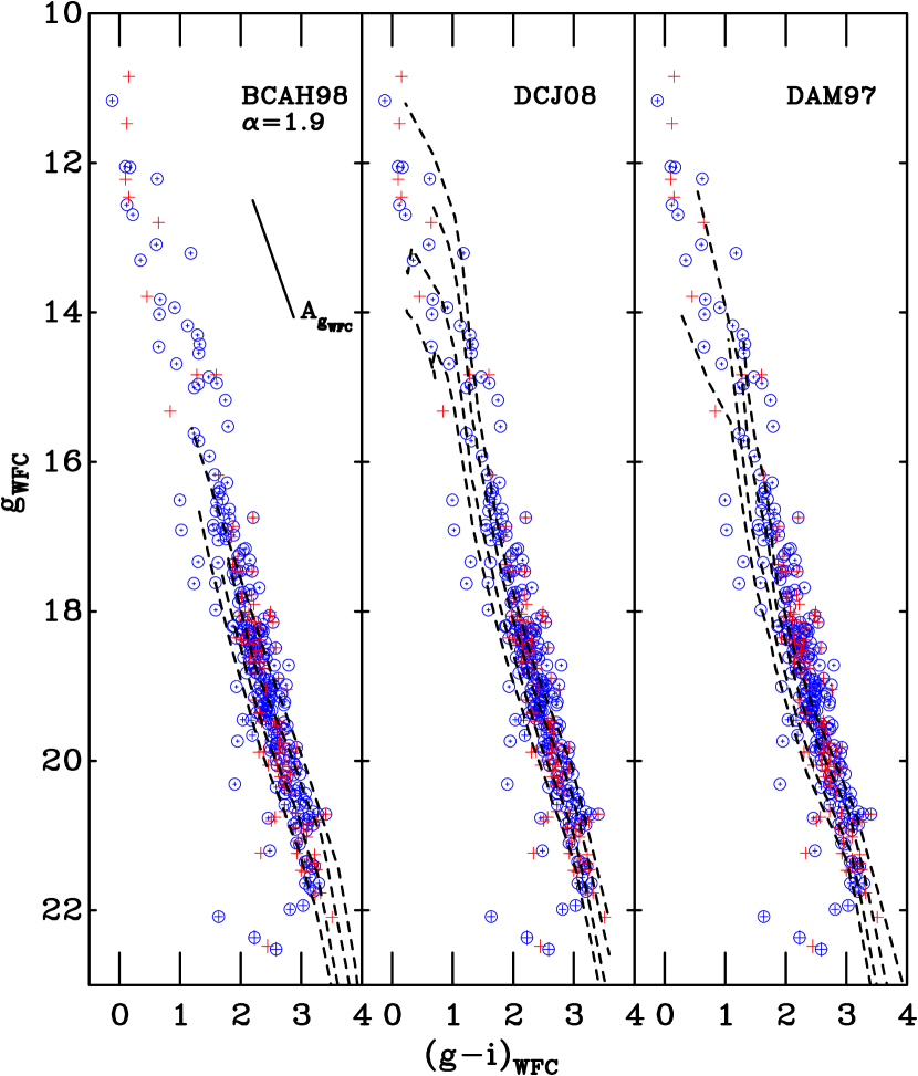
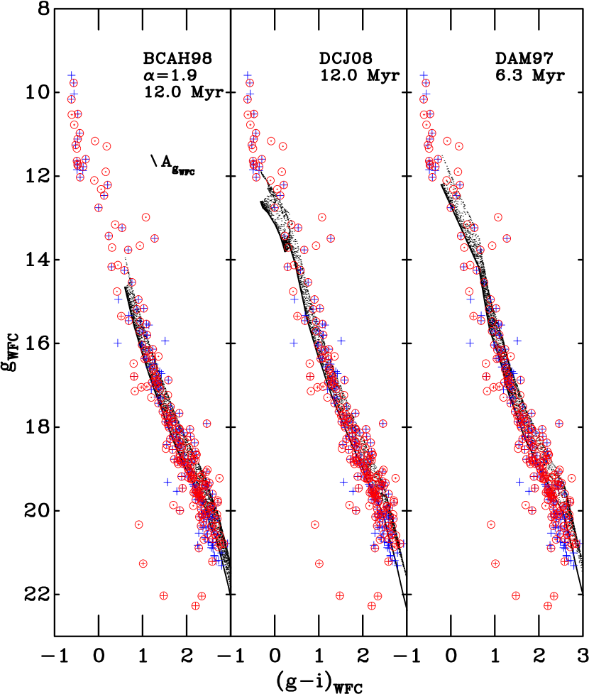
Moving to even younger ages () there are two effects which preclude us using fitting. First, Figs. 8–15 show that for some SFRs with MS ages the semi-empirical pre-MS isochrones do not match the shape of the observed pre-MS locus as well as in the case of the older, more evolved SFRs, with the models tending to cut through the pre-MS locus (see Fig. 8 where this is demonstrated explicitly for the three sets of pre-MS model isochrones using NGC 2244). Second, the observed luminosity spread in CMD space, at a given colour, becomes more pronounced (see Hartmann, 2001 for a discussion on the possible sources). It is apparent from CMDs of some of our SFRs that the observed luminosity spread can be as large as at a given colour, and so although the fitting statistic includes the effects of binarity, this alone is not enough to model the observed spread (see Fig. 9). Given that we have insufficient knowledge of what is causing the observed luminosity spreads in these SFRs (see Section 7.2) as well as lacking the additional data required to accurately model the effects of, for example, stellar variability and accretion, we only use the fitting statistic to derive absolute ages for SFRs where the luminosity spread is commensurate with the two-dimensional model distribution. For SFRs where the observed luminosity spread prohibits the use of the fitting statistic we are unable to derive absolute ages. In such cases, it is possible to a create a relative age ladder of SFRs based on common positions shared in CMD space when compared with a pre-MS model isochrone of a given age (see Fig. 9). Therefore, in Section 6.2 a subset of our sample of SFRs are assigned to such groups and nominal ages for each group discussed.
We have investigated whether using a different technique for SFRs younger than 7 or introduces a discontinuity in our age scale using Ori as an example. For this SFR we find that the fitting statistic derives an age of , whereas the nominal age is (dependent upon the choice of pre-MS model isochrone; see Table 7) and therefore we are confident that the final assigned ages are consistent across the sample and that no discontinuities have been introduced as a result of changing how the pre-MS age has been derived.
6.1 Pre-main-sequence ages derived using
Using the method detailed in the previous section, pre-MS ages have been calculated for the SFRs with MS ages using the fitting statistic in the CMD. The memberships listed in Appendix A have been used to select pre-MS member stars for each SFR.
To fit stars selected as pre-MS members, grids of model distributions were created for each set of interior models spanning a range of ages using the recalibrated BC- relation at the appropriate SFR reddening. For SFRs where we have derived individual star-by-star reddenings for the MS population using the revised Q-method, we adopt the median measured reddening. Although there is a distribution of reddenings due to variable extinction across a given region, the reddening vector in the CMD, and in the mass range we are interested in, lies almost parallel to the observed pre-MS locus and therefore applying a fixed reddening to the pre-MS model distributions does not significantly affect the derived age.
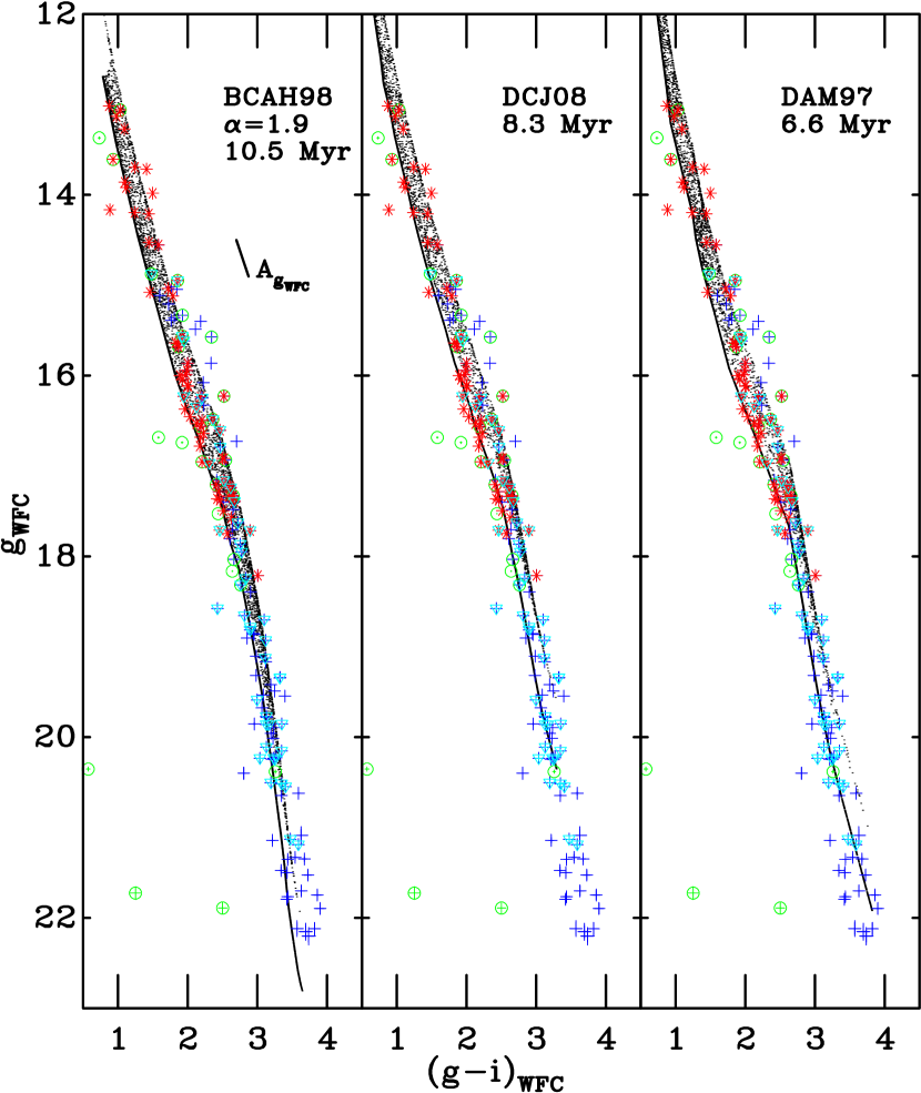
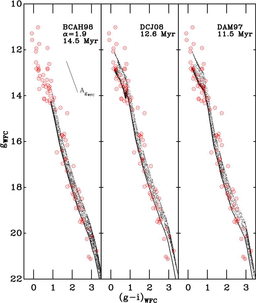
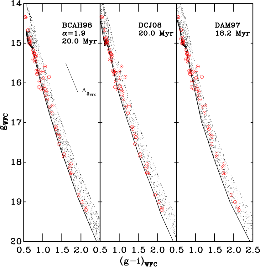
Figs. 10 – 14 shows the CMDs of stars selected as pre-MS members of Ori, NGC 2362, NGC 2169, NGC 7160, and NGC 1960 with the best-fitting BCAH98 , DCJ08 and DAM97 model distributions (including an intrinsic binary fraction of 50 per cent) overlaid at the best-fit MS distance. The largest source of uncertainty in the derived pre-MS age is attributable to the associated uncertainty in the assumed distance, therefore the uncertainty in the pre-MS age is calculated by deriving the corresponding age at the upper and lower distance uncertainty limits as defined by the 68 per cent confidence contour in the MS age-distance grid (see for example Fig. 5). The absolute pre-MS ages for SFRs with MS ages derived using the fitting statistic are shown in Table 6.
| SFR | Absolute Pre-MS Age (Myr) | |||||
|---|---|---|---|---|---|---|
| BCAH98 | DCJ08 | DAM97 | ||||
| Best-fit | 68 per cent | Best-fit | 68 per cent | Best-fit | 68 per cent | |
| Ori | 10.5 | 10.0–11.0 | 8.3 | 7.6–8.7 | 6.6 | 6.0–7.2 |
| NGC 2169 | 12.0 | 10.5–13.2 | 9.1 | 7.9–10.5 | 7.6 | 6.3–8.3 |
| NGC 2362 | 12.0 | 10.5–12.6 | 12.0 | 9.5–12.6 | 6.3 | 5.7–6.6 |
| NGC 7160 | 14.5 | 12.6–16.6 | 12.6 | 11.0–14.5 | 11.5 | 10.5–12.5 |
| NGC 1960 | 20.0 | 19.0–20.9 | 20.0 | 19.0–20.9 | 18.2 | 17.4–19.1 |
6.2 Nominal pre-main-sequence ages
6.2.1 Star-forming regions with main-sequence ages
For the reasons explained in the introduction to Section 6 we derive ages for this group of SFRs by comparing the positions of the observed sequences to a semi-empirical pre-MS single-star model isochrones of a given age. This could be performed by simply de-reddening the pre-MS loci using a given reddening vector and shifting vertically using the derived MS distance, thereby comparing the populations in the absolute magnitude-intrinsic colour plane (e.g. Mayne et al., 2007). However, as was shown in Section 5.1, the reddening and extinction for a given object depends upon its and therefore the reddening vector in the plane is not a fixed vector. As we do not have the necessary diagnostics for the low-mass pre-MS objects in our sample of SFRs, we are unable to de-redden these objects individually. Instead, we leave the sequence in the apparent magnitude-apparent colour plane and the model isochrone is instead reddened using the appropriate reddening and distance modulus for the SFR. By comparing the photometric data to the models in this way SFRs can be grouped in order of increasing age.
As the distance moduli to the SFRs cover a range of the mass regimes probed across the sample of SFRs varies. In addition, there are inherent lower and upper mass limits on the pre-MS interior models, which may further be restricted due to the lowest limit defined by the derived corrections (see Section 5). Of the model isochrones tested, it is clear that the BCAH98 and DCJ08 models represent the best-fit to the observed Pleiades MS for (see Paper 1). Due to the upper mass limit of on the BCAH98 models, the observed pre-MS loci are compared to a semi-empirical DCJ08 single-star model isochrone at an age of . The reason we adopt an age of is that, to within the uncertainties, the ages for SFRs with MS ages are all consistent with , and thus by adopting such an age, we are still assessing whether agreement is observed between age estimates in distinct mass regimes.
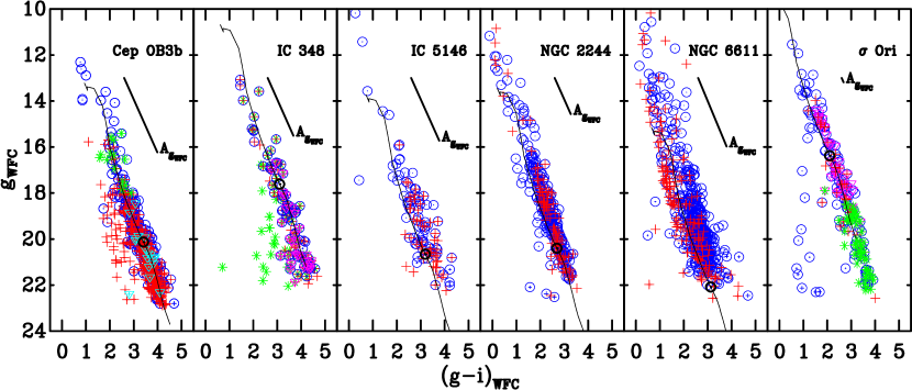
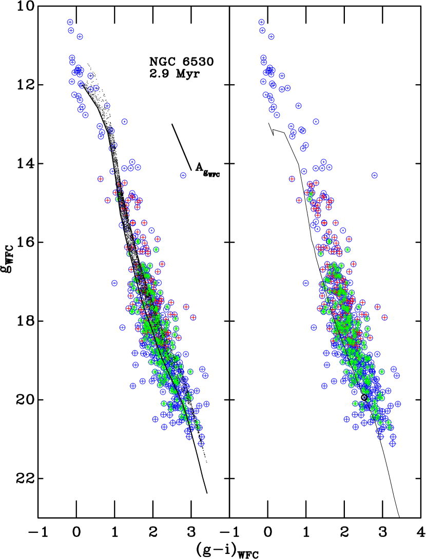
Figs. 9 and 15 shows the CMDs of stars selected as pre-MS members of Cep OB3b, IC 348, IC 5146, NGC 2244, NGC 6530, NGC 6611, and Ori with a semi-empirical DCJ08 single-star isochrone overlaid. It is clear that, for SFRs with MS ages , these can be separated into two distinct groups based on the comparison of the pre-MS populations with the model isochrone. In ascending age order these two groups comprise;
-
•
NGC 6611, IC 5146, NGC 6530, and NGC 2244 – for which the isochrone sits below the observed pre-MS locus,
-
•
Cep OB3b, Ori, and IC 348 – for which the isochrone sits approximately in the middle of the observed pre-MS locus.
| SFR | Nominal Pre-MS Age ( Myr) | ||
| BCAH98 | DCJ08 | DAM97 | |
| NGC 6611(1) | 2 | 1 | 0.5 |
| IC 5146 | 2 | 1 | 0.5 |
| NGC 6530 | 3 | 2 | 1 |
| NGC 2244 | 3 | 2 | 1 |
| Ori | 6 | 5 | 3 |
| IC 348 | 7 | 6 | 4 |
| Cep OB3b | 7 | 7 | 3 |
Due to the fact that, in some cases, the semi-empirical pre-MS isochrones do not follow the shape of the observed pre-MS locus (see for example Fig. 8), and that the mass ranges sampled are different due to the differences in the distance between the SFRs, a pre-MS age derived by simply laying an isochrone over the photometric data will be biased depending on which section of the sequence is fitted. Therefore, a more consistent approach is to estimate the pre-MS age of a given SFR by comparing the position of a model star of given mass (having applied the reddening and distance modulus as for the comparison with the semi-empirical DCJ08 single-star pre-MS model isochrone) with the approximate middle of the observed pre-MS locus. Such ages are termed nominal ages and estimated adopting a mass of . Table 7 shows the nominal pre-MS ages for the SFRs with MS ages .
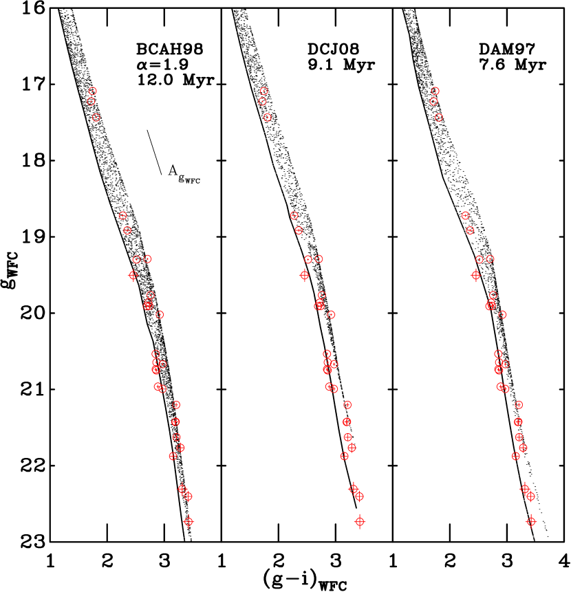
6.2.2 Per
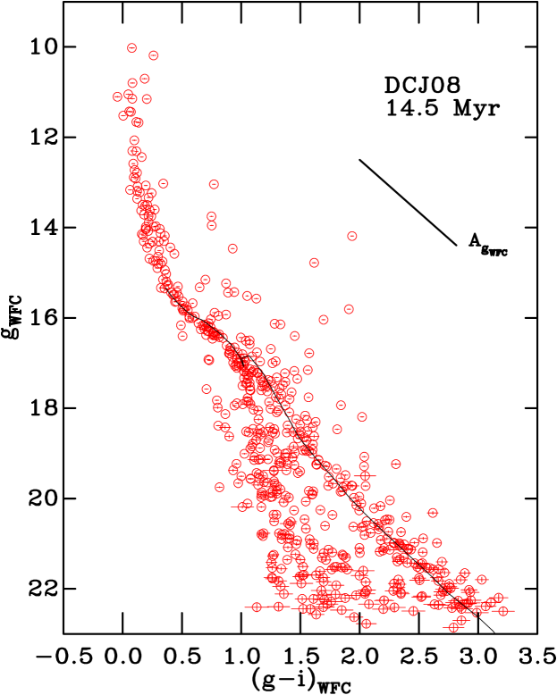
Per could not be fitted using the simple model that accounts for a non-member population as the fraction of non-members (introduced by the selection based purely on positions on the sky relative to the cluster centre; see Appendix A.2) was simply too high. Given the derived best-fit MS age of , one learns nothing by comparing the pre-MS locus with a pre-MS model isochrone. Therefore, in Fig. 16 the semi-empirical DCJ08 single-star model isochrone at an age of is overlaid adopting the best-fit MS distance modulus and reddened by the median value of according to the prescription described in Section 5.1.
From Fig. 16 it is apparent that the semi-empirical DCJ08 single-star model isochrone matches the shape of the observed pre-MS well across the entire colour range, as well as following the sequence across the pre-MS-MS transition. The nominal ages for Per based on the three semi-empirical pre-MS models are for both the BCAH98 and DCJ08 isochrones, and for the DAM97 isochrones. Thus, the consistency demonstrated for the other SFRs with MS ages is still evident for the BCAH98 and DCJ08 models, whereas for the DAM97 models the tendancy to predict a slightly younger age is again observed.
6.3 The effects of assumptions on the pre-main-sequence ages
When deriving ages from the pre-MS photometric data, either by using fitting to the full two-dimensional CMD distribution, or by comparing the sequence with a single-star model isochrone, we have made two main assumptions. First, for SFRs where we have identified the reddening to be spatially variable, we have adopted the median value for fitting the pre-MS. Second, we have assumed the same (solar) composition for all SFRs.
6.3.1 Differential reddening
In a CMD the reddening vector is roughly parallel to the pre-MS (see Fig. 15), much as in the commonly used CMD (e.g. Hillenbrand, 1997; Burningham et al., 2003). Thus the primary effect of variable extinction is to scatter stars along the isochrone. To test how far mis-measured extinction might affect our results, the NGC 7160 pre-MS data were fitted as described in Section 6.1, but using reddening that was 50 per cent larger than the median value () originally used. The reason we adopt NGC 7160 is that this SFR has the largest and most variable reddening of all the SFRs with MS ages . At the best-fit MS distance, the best-fit pre-MS age differs by only 5 per cent. The effect of a scatter will be considerably less than that of a global shift, thus the fact that we have adopted the median reddening for a given SFR, does not significantly affect the derived pre-MS ages.
6.3.2 Composition variations
In the pre-MS regime, we are unable to use sub- or super-solar metallicity pre-MS evolutionary models to derive ages because; i) the DAM97 pre-MS models are only available with a solar composition and ii) although the BCAH98 and DCJ08 models are available for a range of metallicities, we do not have the requisite photometric data in the INT-WFC system to calculate the empirical corrections to the theoretical BC- relation as we have done using the Pleiades for the solar metallicity case (see Section 5). In the MS regime, however, the Schaller et al. (1992) models do cover a range of metallicities and it is possible to investigate what effects adopting a different composition would have on the derived MS parameters.
As an example, we have investigated these effects using NGC 2244 as there is evidence that the metallicity for this SFR could be sub-solar (; see Paunzen et al., 2010). The reddening vectors and BC- relation were recalculated using the atlas9/ODFnew atmospheric models (the closest to the required sub-solar composition from the available grid). The Schaller et al. (1992) interior models (the closest to the sub-solar composition) were used to calculate the reddening, distance, and age as described in Section 4. A revised distance modulus was calculated, whereas both the age and reddening (both median and full range) were insensitive to changes in the metallicity. Hence, if the composition of NGC 2244 is indeed approximately , the distance modulus would be smaller. Whilst sub-solar composition pre-MS model isochrones, at a given age, are more luminous than solar metallicity models in CMD space, it is hard to quantify how the difference in the derived distance modulus would translate into an age difference in absolute terms when fitting the pre-MS population.
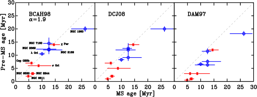
7 Comparing the main-sequence and pre-main-sequence ages
Having derived ages from the MS and pre-MS members for the sample of SFRs, it is now possible to bring these two age diagnostics together. In Sections 6.1 and 6.2 it was shown that the pre-MS ages for young SFRs are heavily model-dependent, even after recalibrating the transformation between theoretical H-R and observable CMD space using the observed colours of Pleiades members. Hence to choose between the various pre-MS age scales, in Fig. 17 we have plotted the MS ages against the pre-MS ages for our sample of SFRs.
The most obvious conclusion that can be drawn from Fig. 17 is that the DAM97 pre-MS age scale is inconsistent with the MS age scale across almost the entire sample. That the DAM97 models tend to predict younger pre-MS ages than other pre-MS models is not a new finding (see for example Dahm, 2005). For a given age, the DAM97 models predict pre-MS stars that are overluminous across a mass range of with respect to both the BCAH98 and DCJ08 models, resulting in an approximate difference of a factor of two in age through isochrone fitting for SFRs with ages .
The levels of agreement between the MS age scale and the pre-MS age scales of BCAH98 and DCJ08 are much higher than for the DAM97 models. For SFRs with pre-MS ages of (on the BCAH98 and DCJ08 scales) both models predict pre-MS ages that are generally consistent with the MS ages derived in Section 4.3. However, for the very youngest clusters () there remains a discrepancy between the two age diagnostics, with the MS ages being approximately a factor of 2 older than the pre-MS ages. The work presented in this paper has therefore removed the age discrepancy between the MS and pre-MS for all but the very youngest SFRs, a significant improvement over the result of Naylor (2009) where a factor 2 discrepancy was still observed at ages of . That we have found agreement between the MS and pre-MS ages (for SFRs with ages ), which are based on different mass regimes that rely on different aspects of stellar physics, instils confidence in the pre-MS ages derived using the BCAH98 and DCJ08 model isochrones.
This agreement between pre-MS and MS ages builds upon that already demonstrated by Pecaut et al. (2012). A detailed analysis of stars hotter than , which should therefore be comparable with our age scale, showed they were a factor of 2.5 less luminous compared with predictions for a old population by four sets of pre-MS evolutionary models. Deriving isochronal ages separately for B-, A-, F-, and G-type stars, as well as the M-type supergiant Antares, Pecaut et al. (2012) not only calculated consistent ages from the pre-MS and post-MS populations, but also increased the age of Upper Sco by approximately a factor of 2, calculating a revised mean age of . Thus these combined works have increased the number of SFRs with significantly revised ages to 14, thereby lending support to the claim of Pecaut et al. (2012) that similarly aged SFRs may be in need of further investigation and possible amendment.
7.1 Final assigned ages
Having demonstrated that the BCAH98 and DCJ08 and MS age scales are generally consistent, we are now in a position to assign the finalised age to each of the 13 SFRs in our sample. As discussed in Section 1, the MS ages are much more uncertain in a statistical sense but on average they confirm that the pre-MS ages, which are statistically much more precise but potentially have more systematic error, are on a reasonable scale. Given that the differences between the pre-MS ages derived using the BCAH98 and DCJ08 models, are typically of the order of , we adopt the mean of these two ages for a given SFR.
There is still the question of what age to assign for the youngest SFRs (pre-MS ages ). Given the uncertainties in the distance to each of the SFRs, the nominal ages given in Table 7 are consistent with two groups of clusters at ages of 2 and . For the group, the MS ages are consistent with the pre-MS nominal ages, and so our final assigned age for this group is . For the very youngest group, the MS ages () are approximately a factor of two greater than the pre-MS ages. For reasons we discuss in Section 7.2 we adopt an age of for this group. The resulting ages we propose should be used for these SFRs in further studies are given in Table 8.
| Age (Myr) | SFR | Distance modulus | |
| 2 | NGC 6611 (Eagle Nebula; M 16)(1,2) | 0.71 | |
| IC 5146 (Cocoon Nebula)(1) | 0.75 | ||
| NGC 6530 (Lagoon Nebula; M 8)(1) | 0.32 | ||
| NGC 2244 (Rosette Nebula)(1) | 0.43 | ||
| 6 | Ori(1) | 0.05 | |
| Cep OB3b(1) | 0.89 | ||
| IC 348(1) | 0.69 | ||
| 10 | Ori (Collinder 69)(1) | 0.11 | |
| 11 | NGC 2169 | 0.16 | |
| 12 | NGC 2362 | 0.07 | |
| 13 | NGC 7160(1) | 0.37 | |
| 14 | Per (NGC 884)(1) | 0.52 | |
| 20 | NGC 1960 (M 36) | 0.20 |
7.2 Discussion
On the balance of the evidence presented in Sections 4.3 and 6.2.1, how reasonable is the distinction between the and groups? Although it is statistically impossible to differentiate between these two groups based on their MS ages (all clustered around ) there is an obvious difference in the luminosity of the pre-MS locus between those SFRs where an isochrone of lies systematically below the observed pre-MS locus and those SFRs where the isochrone traces the approximate middle of the locus. Furthermore, there is a visible difference between the magnitude of the observed luminosity spread between the and groups. For a given colour, the spread in the group covers approximately , whereas in the group the observed spread is approximately a magnitude smaller. Note also that in the older SFRs this spread almost entirely vanishes and is explainable by the presence of binaries and higher order multiple systems.
The main difference between the absolute pre-MS ages derived using the fitting statistic and the nominal pre-MS ages is that the former include an intrinsic binary fraction whereas the latter do not and are solely based on comparison with a single-star model isochrone. Thus, there is a suggestion that the pre-MS ages for both the 2 and groups require a correction to account for binarity. The difference between the lower single-star and upper equal-mass binary envelopes in a coeval model isochrone is , and so if we naïvely assume the most extreme case (i.e. 50 per cent of stars are single and 50 per cent are in equal-mass binaries) this would necessitate that the single-star isochronal ages be increased by a factor that translates to a shift of fainter. For more realistic mass ratio distributions, however, this shift would be smaller. Adopting the most extreme case, such a shift would increase the pre-MS ages for the 2 and groups by an additional factor of . This would have the effect of decreasing the disparity between the MS and pre-MS ages for the group, whilst causing disagreement between the two ages for the group.
Such a shift appears unlikely given that at ages of we would expect to see evolved high-mass stars in SFRs like Cep OB3b, however these are not observed in the optical CMDs. Furthermore, the group represents the earliest visible stages of the star formation process and any shift would increase the age of these SFRs to , suggesting that only after such times do embedded protostars become optically visible.
Any possible quantification of the shift in the ages due to binarity are hampered by the underlying uncertainty in the causes of the observed luminosity spread and the resulting implications for the evolution of single- and binary-star systems (e.g. Preibisch, 2012). In addition, these young SFRs likely contain significant numbers of stars with circumstellar discs, thus further complicating the issue due to the effects of accreting objects observed with a range of accretion rates and viewing angles (see Mayne & Harries, 2010).
In Section 4.2.3 we briefly discussed the uncertainty associated with the distance derived from MS fitting arising from possible variations in towards very young SFRs. The revised ages given in Section 7.1 demonstrate that we have derived consistent ages from both the high-mass and low-mass populations for a range of SFRs down to ages of . There is still, however, disparity between these two ages for the very youngest SFRs (the so-called group) for which the pre-MS ages are approximately factors of between 2 and 3 younger. Given the degeneracy between age and distance in deriving ages using pre-MS evolutionary models, it would be interesting to note whether variations in as a function of age are observed. If this is the case, and the typical value of is larger in the youngest SFRs, then the derived distance would be smaller than that derived in Section 4.3 by a factor of . This could offer a simple solution to the disparity of the MS and pre-MS ages for the youngest SFRs as a decreased distance would necessitate an older age to fit a given photometric pre-MS locus in CMD space, however, further observational work is required in such SFRs to ascertain whether or not this is in fact the case.
We could improve on our work if we understood the observed luminosity spread as well as the problems associated with the evolutionary models and physical processes that affect the associated spectral energy distributions (SEDs) of young pre-MS stars. The models adopted in this study all assume that the mixing-length parameter is constant for all evolutionary stages and identical for all masses. Studies investigating whether this is a reasonable assumption (e.g. Ludwig, Freytag, & Steffen, 1999, 2008) have found that can vary as a function of spectral type, the effects of which would be more pronounced at earlier evolutionary phases where the stars are fully convective and the superadiabatic region is more extended. In addition to inadequacies in the theoretical models (see Baraffe et al., 2002), there are also physical processes that affect the SEDs associated with pre-MS stars, and these can be almost impossible to incorporate into evolutionary codes. An obvious example is the enhanced levels of activity observed on pre-MS stars. High levels of activity, presumably driven by intense surface magnetic fields, can inhibit convective flows at the stellar surface and result in starspots covering a large fraction of the photosphere. Thus the colours of young low-mass stars can be somewhat different than the colours of older stars of the same mass and (e.g. Stauffer et al., 2003). An additional consequence of the inhibited convective flows is that the radii and of stars with intense magnetic fields can differ from stars of a similar mass but with a much weaker magnetic field (e.g. Chabrier, Gallardo, & Baraffe, 2007; Yee & Jensen, 2010). These combined effects further complicate the transformation from H-R to CMD space i.e. for a star of given mass, age, metallicity, and log there is not a single conversion from, for example, to , but instead a range.
In addition to the effects discussed above, there is a fierce debate about whether on-going or early episodes of accretion can result in a marked alteration to the luminosity of very young () objects, when compared to the standard non-accreting models (e.g. Baraffe, Chabrier, & Gallardo, 2009; Hosokawa, Offner, & Krumholz, 2011). Short-lived phases of intense accretion during the early Class I phase of a YSO have been advocated as a possible explanation for the observed luminosity spreads in CMDs of young SFRs. This would naturally impact on the derived ages (and masses) for young objects derived from CMDs, however, this is further compounded by the fact that it is not the currently observed properties that ultimately affects the position of a given object in CMD space, but rather, the accretion history of that specific object. Observational evidence pertaining to effects on the luminosity evolution of young pre-MS objects as a result of accretion history has been reported by Littlefair et al. (2011), and therefore it is conceivable that a considerable portion of the observed luminosity spread in CMDs of young SFRs may be due to such variable accretion histories within a coeval stellar population.
8 Implications
In Section 7.1 a set of revised ages were assigned to a range of young SFRs. Two areas of pre-MS evolution that are heavily dependent upon the adopted ages are; i) the survival timescales for circumstellar discs and ii) the evolutionary timescales of YSOs. Therefore, in this section we discuss the implications of the revised age scale in terms of these two aspects.
8.1 Circumstellar disc lifetimes
Circumstellar discs appear to be a ubiquitous by-product of the star formation process and are a driving factor in the evolution of stars and planetary systems. Mid- to far-IR Spitzer observations of low-mass pre-MS stars indicate that by approximately 80 per cent of primordial discs have dissipated (e.g. Carpenter et al., 2006; Dahm & Hillenbrand, 2007), agreeing with estimates based on near-IR observations (e.g. Haisch, Lada, & Lada, 2001; Hillenbrand, 2005). These timescales are almost exclusively based on ages determined from pre-MS isochrone fitting to young stellar populations and thus any revision of pre-MS SFR ages will naturally alter the expected lifetime of circumstellar discs.

Fig. 18 shows the disc frequency of late-type stars (typically mid-K and later) with near-IR excess emission in different SFRs as a function of our revised age. Disc fractions have, in all but one case, been taken from studies based on Spitzer observations including NGC 6611 (Guarcello et al., 2007), IC 5146 (Harvey et al., 2008), NGC 2244 (Balog et al., 2007), Cep OB3b (Allen et al., 2012), NGC 2169 (Hernandez et al. in preparation), Ori (Hernández et al., 2007), IC 348 (Lada et al., 2006), Ori (Barrado y Navascués et al., 2007), NGC 2362 (Dahm & Hillenbrand, 2007), NGC 7160 (Sicilia-Aguilar et al., 2006), Per (Currie et al., 2010), and NGC 1960 (Smith & Jeffries, 2012). Note that in cases where both Spitzer and Haisch et al. (2001) disc fractions are available, those of Spitzer have been adopted as they are less likely to be affected by sensitivity issues, particularly in the -band (see Lyo et al., 2003).
The disc fraction associated with NGC 6530 comes from the study of Prisinzano et al. (2007) who use Two-Micron All-Sky Survey (2MASS) colour-colour diagrams and various Q-indices (analogous to the Johnson Q-index; see Damiani et al., 2006b) to determine stars with excess, which they attribute to circumstellar material. As demonstrated by Kenyon & Gómez (2001), -band photometry is almost essential for constraining the disc bearing population of a given sample of stars. The bandpasses do not extend to long enough wavelengths to unambiguously demonstrate the presence of circumstellar material, whereas observations at wavelengths provide a higher contrast relative to photospheric emission from the central star. Thus the value quoted by Prisinzano et al. (2007) should only be treated as an approximation.
Fig. 18 shows a remarkable correlation between our revised ages for the sample of SFRs and the associated circumstellar disc fraction, strengthening that originally identified by Haisch et al. (2001). The caveat, however, is that despite this correlation there are likely issues arising from; i) differences in the mass range sampled across the SFRs and ii) sensitivity issues for the latest spectral types. Recent evidence suggests that circumstellar disc dispersal timescales are dependent upon the mass of the star, with discs around lower mass stars surviving longer (e.g. Carpenter et al., 2006; Kennedy & Kenyon, 2009). Furthermore, it can be hard to unambiguously disentangle the disc emission from that of the stellar photosphere, especially for M dwarfs (e.g. Ercolano, Clarke, & Robitaille, 2009). Hence, as the spectral type range is unlikely to be identical for all SFRs, this could mean that such effects may modify the correlation. What is clear from Fig. 18 is that circumstellar discs appear to survive longer than previously believed, indicating a disc half-life of with approximately 80 per cent of stars having lost their discs on timescales of .
An important young SFR not included in our sample but that is commonly used to investigate the evolution of pre-MS processes is Upper Sco. This SFR, in addition to Ori, has been used as a benchmark for the study of circumstellar disc lifetimes and fractions. The Spitzer analysis of Carpenter et al. (2006) shows that Upper Sco has a disc fraction (in the same spectral type range as adopted above) of per cent, in good agreement with the disc fractions of both Ori and NGC 2362 (see Fig. 18). Furthermore, using H as a proxy for stars that are actively accreting, Barrado y Navascués et al. (2007) re-analysed the data of Dolan & Mathieu (2001) and found that per cent of stars are actively accreting in Ori (see also Sacco et al., 2008), compared with per cent in Upper Sco (Lodieu, Dobbie, & Hambly, 2011).
As discussed in Ayliffe & Bate (2009), there is a long-standing concern that the timescales required by numerical models to form a gas giant Jupiter-like planet (; Perri & Cameron, 1974; Pollack et al., 1996) may be larger than the observed circumstellar disc lifetimes (; Haisch et al., 2001). Hence the findings presented in this study offer a simple solution to this apparent discrepancy. If the SFRs used to measure the dissipation timescale of circumstellar discs are on average a factor of 2 older, then the discs survive for approximately twice as long and thus provide the necessary reservoirs to form gas giant planets on timescales.
8.2 Evolutionary lifetimes of young stellar objects
Having discussed the effects of the revised age scale in terms of circumstellar disc lifetimes, this naturally leads onto the lifetimes of different evolutionary stages of YSOs. The generally adopted method to derive such timescales is to use the number of objects in each class to establish relative lifetimes (e.g. Wilking, Lada, & Young, 1989). A recent study by Evans et al. (2009) proposed that if star formation is a continuous process with a duration larger than the age of Class II (classical T-Tauri stars), then relative YSO evolutionary lifetimes can be estimated by taking the ratio of objects in each class and multiplying by the adopted lifetime for a Class II object. Based on various studies of young SFRs (see references within Section 5.3 of Evans et al., 2009), a lifetime of was assigned to the Class II evolutionary phase, with the lifetimes of the other classes derived accordingly.
It is clear then that any revision to the pre-MS ages of young SFRs will have an impact on the adopted Class II lifetime used to calculate relative lifetimes for other YSO evolutionary phases. Whilst an in-depth discussion on how the relative ages are affected by the revised ages is beyond the scope of this study, Fig. 18 suggests that the adopted lifetime of Class II objects is likely underestimated. The ages shown in Table 8 are approximately a factor of 2 older than current ages for the same SFRs. Regions such as Ori, with two independent age determinations at (see also Upper Sco; Pecaut et al., 2012) which show that per cent of stars retain their optically thick circumstellar discs (indicative of Class II status) and that per cent of stars are still actively accreting, imply a longer Class II lifetime somewhere in the region of . Propagating this age to the earlier Class I lifetime, based on the number of YSOs presented in Evans et al. (2009) and ignoring environmental effects, indicates an average lifetime of , resulting in a lifetime that is considerably longer than most estimates (cf. ; Hatchell et al., 2007).
9 Conclusions
In this study we have used the stellar populations of 13 young SFRs to critically assess the ages derived using pre-MS isochrones in CMDs. The stages we have gone through to achieve this are as follows.
-
1.
We have derived a self-consistent set of ages, distances and reddenings (with typically higher precision than previous estimates and statistically meaningful uncertainties) by fitting the MS populations of our sample of SFRs with MS evolutionary models. For several of these SFRs, this represents the first parameter derivations in the literature based on a robust statistical fitting technique.
-
2.
We have created new semi-empirical pre-MS isochrones incorporating existing stellar interior models, an empirical BC- relation, and theoretical corrections for the dependence on log. These new isochrones have been used to calculate ages from the pre-MS populations of our sample of SFRs. We find that the ages derived using these semi-empirical isochrones are typically a factor of 2 older than current estimates.
-
3.
Comparing the various pre-MS age scales with the more reliable MS age scale, we find that the DAM97 models systematically underestimate the ages of young SFRs, whereas the scales of both the BCAH98 and DCJ08 models are generally consistent. Thus, we suggest that in an effort to create an absolute pre-MS age scale, either the BCAH98 or DCJ08 models should be adopted for this purpose.
-
4.
We still note a discrepancy between the MS and pre-MS ages for very young SFRs (MS age ) for which the MS ages are approximately factors of between 2 and 3 greater than the pre-MS ages. This mismatch in the ages could be attributed to a combination of inherent uncertainties in the evolutionary models (e.g. the treatment of convection) as well as physical processes that affect the colours of real stars that are not incorporated in the models. Furthermore, sources of systematic uncertainty due to possible variations in the value of for the youngest SFRs and the effects of binarity could contribute to this disparity.
-
5.
We have furthermore investigated the effects of the revised pre-MS age scale in terms of both circumstellar disc lifetimes and YSO evolutionary timescales. We conclude that circumstellar discs survive approximately twice as long as currently believed and that this could offer a practical solution to the apparent discrepancy that the time required to form planets is larger than the lifetime of discs around stars. In addition, we find that due to the revised ages, the typical Class I lifetime is also underestimated, with a significantly longer revised lifetime of suggested.
Acknowledgements
CPMB is funded by a UK Science and Technology Facilities Council (STFC) studentship. SPL is supported by an RCUK fellowship. The authors would like to thank Charles D. H. Williams for maintaining the Xgrid facilities at the University of Exeter which were used to reduce the photometric data presented in this study. We also thank the referee for useful comments and constructive suggestions that have greatly improved this work. This research has made use of data obtained at the Isaac Newton Telescope which is operated on the island of La Palma by the Isaac Newton Group (ING) in the Spanish Observatorio del Roque de los Muchachos of the Institutio de Astrofisica de Canarias. This research has made use of archival data products from the Two-Micron All-Sky Survey (2MASS), which is a joint project of the University of Massachusetts and the Infrared Processing and Analysis Center, funded by the National Aeronautics and Space Administration (NASA) and the National Science Foundation.
References
- Allard et al. (2011) Allard F., Homeier D., Freytag B., 2011, in Astronomical Society of the Pacific Conference Series, Vol. 448, 16th Cambridge Workshop on Cool Stars, Stellar Systems, and the Sun, Johns-Krull C., Browning M. K., West A. A., eds., p. 91
- Allen et al. (2012) Allen T. S., Gutermuth R. A., Kryukova E., Megeath S. T., Pipher J. L., Naylor T., Jeffries R. D., Wolk S. J., Spitzbart B., Muzerolle J., 2012, ApJ, 750, 125
- Ayliffe & Bate (2009) Ayliffe B. A., Bate M. R., 2009, MNRAS, 393, 49
- Balog et al. (2007) Balog Z., Muzerolle J., Rieke G. H., Su K. Y. L., Young E. T., Megeath S. T., 2007, ApJ, 660, 1532
- Baraffe et al. (1998) Baraffe I., Chabrier G., Allard F., Hauschildt P. H., 1998, A&A, 337, 403
- Baraffe et al. (2002) Baraffe I., Chabrier G., Allard F., Hauschildt P. H., 2002, A&A, 382, 563
- Baraffe et al. (2009) Baraffe I., Chabrier G., Gallardo J., 2009, ApJ, 702, L27
- Barrado et al. (2011) Barrado D., Stelzer B., Morales-Calderón M., Bayo A., Huélamo N., Stauffer J. R., Hodgkin S., Galindo F., Verdugo E., 2011, A&A, 526, A21
- Barrado y Navascués et al. (2004) Barrado y Navascués D., Stauffer J. R., Bouvier J., Jayawardhana R., Cuillandre J., 2004, ApJ, 610, 1064
- Barrado y Navascués et al. (2007) Barrado y Navascués D., Stauffer J. R., Morales-Calderón M., Bayo A., Fazzio G., Megeath T., Allen L., Hartmann L. W., Calvet N., 2007, ApJ, 664, 481
- Bell et al. (2012) Bell C. P. M., Naylor T., Mayne N. J., Jeffries R. D., Littlefair S. P., 2012, MNRAS, 424, 3178
- Bessell (1990a) Bessell M. S., 1990a, A&AS, 83, 357
- Bessell (1990b) Bessell M. S., 1990b, PASP, 102, 1181
- Bessell et al. (1998) Bessell M. S., Castelli F., Plez B., 1998, A&A, 333, 231
- Blaauw et al. (1959) Blaauw A., Hiltner W. A., Johnson H. L., 1959, ApJ, 130, 69
- Boss (1997) Boss A. P., 1997, Science, 276, 1836
- Burningham et al. (2003) Burningham B., Naylor T., Jeffries R. D., Devey C. R., 2003, MNRAS, 346, 1143
- Burningham et al. (2005) Burningham B., Naylor T., Littlefair S. P., Jeffries R. D., 2005, MNRAS, 356, 1583
- Cardelli & Clayton (1988) Cardelli J. A., Clayton G. C., 1988, AJ, 95, 516
- Cardelli et al. (1989) Cardelli J. A., Clayton G. C., Mathis J. S., 1989, ApJ, 345, 245
- Cargile & James (2010) Cargile P. A., James D. J., 2010, AJ, 140, 677
- Carpenter et al. (2006) Carpenter J. M., Mamajek E. E., Hillenbrand L. A., Meyer M. R., 2006, ApJ, 651, L49
- Castelli & Kurucz (2004) Castelli F., Kurucz R. L., 2004, in IAU Symposium, Vol. 210, Modelling of Stellar Atmospheres, Piskunov N. E., Weiss W. W., Gray D. F., eds., p. A20
- Chabrier et al. (2007) Chabrier G., Gallardo J., Baraffe I., 2007, A&A, 472, L17
- Cody & Hillenbrand (2010) Cody A. M., Hillenbrand L. A., 2010, ApJS, 191, 389
- Cohen et al. (2004) Cohen R. E., Herbst W., Williams E. C., 2004, AJ, 127, 1602
- Currie et al. (2010) Currie T., Hernandez J., Irwin J., Kenyon S. J., Tokarz S., Balog Z., Bragg A., Berlind P., Calkins M., 2010, ApJS, 186, 191
- Cutri et al. (2003) Cutri R. M., Skrutskie M. F., van Dyk S., et al., 2003, 2MASS Point Source Catalogue. Available at http://www.ipac.caltech.edu/2mass/, Cutri, R. M., et al., ed.
- Dahm (2005) Dahm S. E., 2005, AJ, 130, 1805
- Dahm & Hillenbrand (2007) Dahm S. E., Hillenbrand L. A., 2007, AJ, 133, 2072
- Damiani et al. (2004) Damiani F., Flaccomio E., Micela G., Sciortino S., Harnden Jr. F. R., Murray S. S., 2004, ApJ, 608, 781
- Damiani et al. (2006a) Damiani F., Micela G., Sciortino S., Huélamo N., Moitinho A., Harnden Jr. F. R., Murray S. S., 2006a, A&A, 460, 133
- Damiani et al. (2006b) Damiani F., Prisinzano L., Micela G., Sciortino S., 2006b, A&A, 459, 477
- D’Antona & Mazzitelli (1997) D’Antona F., Mazzitelli I., 1997, Mem. Soc. Astron. Italiana, 68, 807
- Dolan & Mathieu (1999) Dolan C. J., Mathieu R. D., 1999, AJ, 118, 2409
- Dolan & Mathieu (2001) Dolan C. J., Mathieu R. D., 2001, AJ, 121, 2124
- Dotter et al. (2008) Dotter A., Chaboyer B., Jevremović D., Kostov V., Baron E., Ferguson J. W., 2008, ApJS, 178, 89
- Ercolano et al. (2009) Ercolano B., Clarke C. J., Robitaille T. P., 2009, MNRAS, 394, L141
- Evans et al. (2009) Evans II N. J., Dunham M. M., Jørgensen J. K., Enoch M. L., Merín B., van Dishoeck E. F., Alcalá J. M., Myers P. C., Stapelfeldt K. R., Huard T. L., Allen L. E., Harvey P. M., van Kempen T., Blake G. A., Koerner D. W., Mundy L. G., Padgett D. L., Sargent A. I., 2009, ApJS, 181, 321
- Flower (1996) Flower P. J., 1996, ApJ, 469, 355
- Getman et al. (2006) Getman K. V., Feigelson E. D., Townsley L., Broos P., Garmire G., Tsujimoto M., 2006, ApJS, 163, 306
- Greenstein & Wallerstein (1958) Greenstein J. L., Wallerstein G., 1958, ApJ, 127, 237
- Guarcello et al. (2009) Guarcello M. G., Micela G., Damiani F., Peres G., Prisinzano L., Sciortino S., 2009, A&A, 496, 453
- Guarcello et al. (2007) Guarcello M. G., Prisinzano L., Micela G., Damiani F., Peres G., Sciortino S., 2007, A&A, 462, 245
- Guetter (1979) Guetter H. H., 1979, AJ, 84, 1846
- Gullbring et al. (1998) Gullbring E., Hartmann L., Briceño C., Calvet N., Muzerolle J., 1998, in Astronomical Society of the Pacific Conference Series, Vol. 154, Cool Stars, Stellar Systems, and the Sun, R. A. Donahue & J. A. Bookbinder, ed., p. 1709
- Haisch et al. (2001) Haisch Jr. K. E., Lada E. A., Lada C. J., 2001, ApJ, 553, L153
- Hardie et al. (1964) Hardie R. H., Heiser A. M., Tolbert C. R., 1964, ApJ, 140, 1472
- Harris et al. (1954) Harris D. L., Morgan W. W., Roman N. G., 1954, ApJ, 119, 622
- Hartmann (2001) Hartmann L., 2001, AJ, 121, 1030
- Hartmann (2003) Hartmann L., 2003, ApJ, 585, 398
- Harvey et al. (2008) Harvey P. M., Huard T. L., Jørgensen J. K., Gutermuth R. A., Mamajek E. E., Bourke T. L., Merín B., Cieza L., Brooke T., Chapman N., Alcalá J. M., Allen L. E., Evans II N. J., Di Francesco J., Kirk J. M., 2008, ApJ, 680, 495
- Hatchell et al. (2007) Hatchell J., Fuller G. A., Richer J. S., Harries T. J., Ladd E. F., 2007, A&A, 468, 1009
- Henderson & Stassun (2012) Henderson C. B., Stassun K. G., 2012, ApJ, 747, 51
- Herbig (1998) Herbig G. H., 1998, ApJ, 497, 736
- Herbig & Dahm (2002) Herbig G. H., Dahm S. E., 2002, AJ, 123, 304
- Hernández et al. (2007) Hernández J., Calvet N., Briceño C., Hartmann L., Vivas A. K., Muzerolle J., Downes J., Allen L., Gutermuth R., 2007, ApJ, 671, 1784
- Hillenbrand (1997) Hillenbrand L. A., 1997, AJ, 113, 1733
- Hillenbrand (2005) Hillenbrand L. A., 2005, in STSci Symposium Series, Vol. 19, A Decade of Discovery: Planets Around Other Stars, Livio M., ed.
- Hillenbrand et al. (2008) Hillenbrand L. A., Bauermeister A., White R. J., 2008, in Astronomical Society of the Pacific Conference Series, Vol. 384, 14th Cambridge Workshop on Cool Stars, Stellar Systems, and the Sun, G. van Belle, ed., p. 200
- Hillenbrand et al. (1993) Hillenbrand L. A., Massey P., Strom S. E., Merrill K. M., 1993, AJ, 106, 1906
- Hiltner & Johnson (1956) Hiltner W. A., Johnson H. L., 1956, ApJ, 124, 367
- Hiltner & Morgan (1969) Hiltner W. A., Morgan W. W., 1969, AJ, 74, 1152
- Hoag et al. (1961) Hoag A. A., Johnson H. L., Iriarte B., Mitchell R. I., Hallam K. L., Sharpless S., 1961, Publications of the U.S. Naval Observatory Second Series, 17, 1
- Hosokawa et al. (2011) Hosokawa T., Offner S. S. R., Krumholz M. R., 2011, ApJ, 738, 140
- Jeffries et al. (2006) Jeffries R. D., Maxted P. F. L., Oliveira J. M., Naylor T., 2006, MNRAS, 371, L6
- Jeffries et al. (2013) Jeffries R. D., Naylor T., Mayne N. J., Bell C. P. M., Littlefair S. P., 2013, MNRAS submitted
- Jeffries et al. (2007) Jeffries R. D., Oliveira J. M., Naylor T., Mayne N. J., Littlefair S. P., 2007, MNRAS, 376, 580
- Jeffries et al. (2001) Jeffries R. D., Thurston M. R., Hambly N. C., 2001, A&A, 375, 863
- Johnson (1962) Johnson H. L., 1962, ApJ, 136, 1135
- Johnson (1966) Johnson H. L., 1966, ARA&A, 4, 193
- Johnson & Morgan (1953) Johnson H. L., Morgan W. W., 1953, ApJ, 117, 313
- Johnson & Morgan (1955) Johnson H. L., Morgan W. W., 1955, ApJ, 122, 429
- Kennedy & Kenyon (2009) Kennedy G. M., Kenyon S. J., 2009, ApJ, 695, 1210
- Kenyon et al. (2005) Kenyon M. J., Jeffries R. D., Naylor T., Oliveira J. M., Maxted P. F. L., 2005, MNRAS, 356, 89
- Kenyon & Gómez (2001) Kenyon S. J., Gómez M., 2001, AJ, 121, 2673
- Kenyon & Hartmann (1995) Kenyon S. J., Hartmann L., 1995, ApJS, 101, 117
- Lada & Adams (1992) Lada C. J., Adams F. C., 1992, ApJ, 393, 278
- Lada et al. (2006) Lada C. J., Muench A. A., Luhman K. L., Allen L., Hartmann L., Megeath T., Myers P., Fazio G., Wood K., Muzerolle J., Rieke G., Siegler N., Young E., 2006, AJ, 131, 1574
- Lejeune & Schaerer (2001) Lejeune T., Schaerer D., 2001, A&A, 366, 538
- Linsky et al. (2007) Linsky J. L., Gagné M., Mytyk A., McCaughrean M., Andersen M., 2007, ApJ, 654, 347
- Littlefair et al. (2005) Littlefair S. P., Naylor T., Burningham B., Jeffries R. D., 2005, MNRAS, 358, 341
- Littlefair et al. (2011) Littlefair S. P., Naylor T., Mayne N. J., Saunders E., Jeffries R. D., 2011, MNRAS, 413, L56
- Littlefair et al. (2010) Littlefair S. P., Naylor T., Mayne N. J., Saunders E. S., Jeffries R. D., 2010, MNRAS, 403, 545
- Lodieu et al. (2011) Lodieu N., Dobbie P. D., Hambly N. C., 2011, A&A, 527, A24
- Ludwig et al. (2008) Ludwig H.-G., Caffau E., Kučinskas A., 2008, in IAU Symposium, Vol. 252, The Art of Modelling Stars in the 21st Century, Deng L., Chan K. L., eds., p. 75
- Ludwig et al. (1999) Ludwig H.-G., Freytag B., Steffen M., 1999, A&A, 346, 111
- Luhman et al. (2005a) Luhman K. L., Lada E. A., Muench A. A., Elston R. J., 2005a, ApJ, 618, 810
- Luhman et al. (2005b) Luhman K. L., McLeod K. K., Goldenson N., 2005b, ApJ, 623, 1141
- Luhman et al. (2003) Luhman K. L., Stauffer J. R., Muench A. A., Rieke G. H., Lada E. A., Bouvier J., Lada C. J., 2003, ApJ, 593, 1093
- Lyo et al. (2003) Lyo A., Lawson W. A., Mamajek E. E., Feigelson E. D., Sung E., Crause L. A., 2003, MNRAS, 338, 616
- Lyra et al. (2006) Lyra W., Moitinho A., van der Bliek N. S., Alves J., 2006, A&A, 453, 101
- Mayne & Harries (2010) Mayne N. J., Harries T. J., 2010, MNRAS, 409, 1307
- Mayne & Naylor (2008) Mayne N. J., Naylor T., 2008, MNRAS, 386, 261
- Mayne et al. (2007) Mayne N. J., Naylor T., Littlefair S. P., Saunders E. S., Jeffries R. D., 2007, MNRAS, 375, 1220
- Murdin & Penston (1977) Murdin P., Penston M. V., 1977, MNRAS, 181, 657
- Naylor (2009) Naylor T., 2009, MNRAS, 399, 432
- Naylor & Fabian (1999) Naylor T., Fabian A. C., 1999, MNRAS, 302, 714
- Naylor & Jeffries (2006) Naylor T., Jeffries R. D., 2006, MNRAS, 373, 1251
- Naylor & Mayne (2010) Naylor T., Mayne N. J., 2010, Highlights of Astronomy, 15, 763
- Naylor et al. (2002) Naylor T., Totten E. J., Jeffries R. D., Pozzo M., Devey C. R., Thompson S. A., 2002, MNRAS, 335, 291
- Ogura et al. (2002) Ogura K., Sugitani K., Pickles A., 2002, AJ, 123, 2597
- Oke & Gunn (1983) Oke J. B., Gunn J. E., 1983, ApJ, 266, 713
- Orsatti et al. (2000) Orsatti A. M., Vega E. I., Marraco H. G., 2000, A&AS, 144, 195
- Orsatti et al. (2006) Orsatti A. M., Vega E. I., Marraco H. G., 2006, AJ, 132, 1783
- Paunzen et al. (2010) Paunzen E., Heiter U., Netopil M., Soubiran C., 2010, A&A, 517, A32
- Pecaut et al. (2012) Pecaut M. J., Mamajek E. E., Bubar E. J., 2012, ApJ, 746, 154
- Perri & Cameron (1974) Perri F., Cameron A. G. W., 1974, Icarus, 22, 416
- Piskunov et al. (2004) Piskunov A. E., Belikov A. N., Kharchenko N. V., Sagar R., Subramaniam A., 2004, MNRAS, 349, 1449
- Pollack (1984) Pollack J. B., 1984, ARA&A, 22, 389
- Pollack et al. (1996) Pollack J. B., Hubickyj O., Bodenheimer P., Lissauer J. J., Podolak M., Greenzweig Y., 1996, Icarus, 124, 62
- Pozzo et al. (2003) Pozzo M., Naylor T., Jeffries R. D., Drew J. E., 2003, MNRAS, 341, 805
- Preibisch (2012) Preibisch T., 2012, Research in Astronomy and Astrophysics, 12, 1
- Preibisch & Zinnecker (2002) Preibisch T., Zinnecker H., 2002, AJ, 123, 1613
- Prisinzano et al. (2007) Prisinzano L., Damiani F., Micela G., Pillitteri I., 2007, A&A, 462, 123
- Prisinzano et al. (2005) Prisinzano L., Damiani F., Micela G., Sciortino S., 2005, A&A, 430, 941
- Röser et al. (2010) Röser S., Demleitner M., Schilbach E., 2010, AJ, 139, 2440
- Sacco et al. (2008) Sacco G. G., Franciosini E., Randich S., Pallavicini R., 2008, A&A, 488, 167
- Sanner et al. (2000) Sanner J., Altmann M., Brunzendorf J., Geffert M., 2000, A&A, 357, 471
- Sanz-Forcada et al. (2004) Sanz-Forcada J., Franciosini E., Pallavicini R., 2004, A&A, 421, 715
- Schaller et al. (1992) Schaller G., Schaerer D., Meynet G., Maeder A., 1992, A&AS, 96, 269
- Schmidt-Kaler (1982) Schmidt-Kaler T., 1982, in Landolt-Börnstein, Neue Serie VI/2b, 453, 15
- Sicilia-Aguilar et al. (2006) Sicilia-Aguilar A., Hartmann L., Calvet N., Megeath S. T., Muzerolle J., Allen L., D’Alessio P., Merín B., Stauffer J., Young E., Lada C., 2006, ApJ, 638, 897
- Sicilia-Aguilar et al. (2004) Sicilia-Aguilar A., Hartmann L. W., Briceño C., Muzerolle J., Calvet N., 2004, AJ, 128, 805
- Sicilia-Aguilar et al. (2005) Sicilia-Aguilar A., Hartmann L. W., Hernández J., Briceño C., Calvet N., 2005, AJ, 130, 188
- Siess et al. (2000) Siess L., Dufour E., Forestini M., 2000, A&A, 358, 593
- Slesnick et al. (2002) Slesnick C. L., Hillenbrand L. A., Massey P., 2002, ApJ, 576, 880
- Smith & Jeffries (2012) Smith R., Jeffries R. D., 2012, MNRAS, 420, 2884
- Stauffer et al. (2003) Stauffer J. R., Jones B. F., Backman D., Hartmann L. W., Barrado y Navascués D., Pinsonneault M. H., Terndrup D. M., Muench A. A., 2003, AJ, 126, 833
- Stauffer et al. (1998) Stauffer J. R., Schild R., Barrado y Navascues D., Backman D. E., Angelova A. M., Kirkpatrick J. D., Hambly N., Vanzi L., 1998, ApJ, 504, 805
- Uribe et al. (2002) Uribe A., García-Varela J., Sabogal-Martínez B., Higuera G. M. A., Brieva E., 2002, PASP, 114, 233
- van den Ancker et al. (1997) van den Ancker M. E., The P. S., Feinstein A., Vazquez R. A., de Winter D., Perez M. R., 1997, A&AS, 123, 63
- Walker (1957) Walker M. F., 1957, ApJ, 125, 636
- Walker (1959) Walker M. F., 1959, ApJ, 130, 57
- Walker (1961) Walker M. F., 1961, ApJ, 133, 438
- Wang et al. (2008) Wang J., Townsley L. K., Feigelson E. D., Broos P. S., Getman K. V., Román-Zúñiga C. G., Lada E., 2008, ApJ, 675, 464
- White et al. (1999) White R. J., Ghez A. M., Reid I. N., Schultz G., 1999, ApJ, 520, 811
- Wildey (1963) Wildey R. L., 1963, AJ, 68, 190
- Wilking et al. (1989) Wilking B. A., Lada C. J., Young E. T., 1989, ApJ, 340, 823
- Yee & Jensen (2010) Yee J. C., Jensen E. L. N., 2010, ApJ, 711, 303
Appendix A Pre-main-sequence literature memberships
Many of the SFRs investigated in this study lie in or near the Galactic plane and as such a CMD for a given field-of-view will contain a high number of field stars. Thus we must consider the issue of identifying and isolating bona fide pre-MS members.
Pre-MS stars exhibit several characteristics that highlight their youth and which can be used to differentiate between them and older field stars. These indicators only differentiate between different types of stellar populations and not between distinct young populations (see Jeffries et al., 2006). Where no literature memberships were available, we instead adopted an approach based on relative positions on the sky to identify possible members, however this has the obvious drawback of including a number of non-members in the selection.
A.1 Cep OB3b
X-ray members are from Naylor & Fabian (1999) and Getman et al. (2006) using the ROSAT PSPC and Chandra ACIS instruments respectively. We used a combination of both as the area covered by the ROSAT pointing is larger than the Chandra field-of-view. For stars common to both catalogues, we adopt the positions from the Chandra dataset due to the improved spatial resolution and sensitivity.
Spectroscopic members are taken from Pozzo et al. (2003). They took spectra of objects within an initial photometric cut made in the CMD, using a colour-colour diagram of optical counterparts to the Naylor & Fabian (1999) ROSAT sources to identify regions with a high fraction of probable members. Spectroscopic follow-up measurements provided lithium equivalent widths (), , and radial velocities. Memberships were assigned based on the comparison between individual radial velocities and the group mean, in addition to strong spectroscopic features. Additional H members are from Ogura et al. (2002) which comprise a subset of a Herbig-Haro object survey using a narrowband H filter.
Periodic variables are from an -band variability study by Littlefair et al. (2010). A recent Spitzer IRAC and MIPS study (Allen et al., 2012) has demonstrated that the young stars within the cluster are concentrated into two sub-clusters; an eastern sub-cluster near the Cep B molecular cloud and a western sub-cluster near the Cep F molecular cloud. The literature memberships listed above only cover the eastern sub-cluster, whereas the variability study of Littlefair et al. (2010) covers both sub-clusters. To not bias the selection of pre-MS members, the positions on the sky of the other literature sources were used to define a region within which variability members were isolated.
A.2 Per
There is a lack of bona fide pre-MS member diagnostics for Per. The so-called spectroscopically confirmed members of Currie et al. (2010) are not based on the presence of spectral features (e.g. Li I or H) but represent a sequence defined by a combined MS and pre-MS isochrone in the de-reddened -band magnitude versus spectral type diagram. The width of this sequence was determined by; i) the physical extent of the cluster, ii) binarity, and iii) uncertainties in the derived spectral types. Cross-correlation of the Currie et al. (2010) members with our optical photometric catalogue results in a poorly defined pre-MS locus with less than 10 stars occupying the single-star sequence at magnitudes .
Our photometric catalogue extends to and therefore stellar positions on the sky were instead used to choose an area that minimises foreground and background contamination (see Mayne et al., 2007). Stars brighter than lie bluewards of the contamination and thus represent a subset of the Per stellar population where the field star contamination is minimal. The positions of these stars were then overlaid on the positions of the entire photometric catalogue and circular positional selections from down to in increments of were made around the central cluster coordinates of (Mayne et al., 2007). The resulting sequence was visually inspected (by-eye) and the best results (fraction of candidate member-to-field stars) was found for a radius of . To ensure that the selection of the cluster centre was not biased, the positions of proper motion members from Uribe et al. (2002) and likely members based on spectral types from Slesnick, Hillenbrand, & Massey (2002) were also overlaid. In both cases, the central coordinates from each source were almost identical.
A.3 IC 348
members are taken from Herbig (1998) who carried out a wide-field grism spectrograph survey of the region, discarding stars with . Spectral types (through comparison with dwarf spectral standards) and extinctions were derived for 80 of these stars using follow-up spectroscopy. Additional spectroscopic members are taken from Luhman et al. (2003, 2005a, 2005b). Memberships were assigned using a combination of spectral types, spectral features (H, Na I, and K I), and positions within extinction-corrected CMDs.
X-ray members are from Preibisch & Zinnecker (2002) taken with the Chandra ACIS detector (supplemented with additional data from the Second ROSAT PSPC catalogue777http://ledas-www.star.le.ac.uk/rosat/rra/).
A.4 IC 5146
members are taken from Herbig & Dahm (2002) who conducted a wide-field grism spectrograph survey to identify emission stars to a limit of and limiting magnitude of . Only stars with and which lie above the Pleiades MS at a distance of as described in Herbig & Dahm (2002) were used.
Additional IR excess members are based on the Spitzer IRAC and MIPS photometry of Harvey et al. (2008). The identification of YSOs from Spitzer is generally based on some combination of IR excess in addition to a brightness limit (set by the limiting magnitude fainter than which extragalactic contamination becomes too high to reliably distinguish between objects). A combination of colour-colour diagrams and CMDs were used to identify predominantly Class I and Class II objects.
A.5 Ori
Li I abundance members come from Dolan & Mathieu (2001), extending the previous study of Dolan & Mathieu (1999). An initial photometric cut for stars with was made, with the probable members chosen based on their position relative to a isochrone in an CMD. Follow-up spectroscopic measurements were taken and was used as a youth indicator, where stars with were retained as members.
Additional spectroscopic members come from Barrado y Navascués et al. (2004) where optical photometry was combined with 2MASS observations to initially identify possible member candidates in CMD space. Follow-up spectroscopic observations were taken to measure . Memberships were assigned to those stars that satisfied both spectroscopic and photometric criteria. Later, Barrado y Navascués et al. (2007) used Spitzer IRAC photometry to identify probable low-mass members based on IR excess using IRAC colour-colour diagrams in conjunction with optical and IR CMDs. Further members are from the spectroscopic study of Sacco et al. (2008) who measured both and in addition to radial velocities. Final membership is based on a combination of individual candidate velocities that are consistent with the cluster dispersion, the presence of strong and the presence of emission.
X-ray members are taken from Barrado et al. (2011) observed using the XMM-Newton EPIC detector.
A.6 NGC 1960
Spectroscopic members are from an upcoming paper by Jeffries et al. (2013). Optical photometry was used to identify possible cluster members from their position in CMD space, selecting objects with . Spectroscopic observations were to identify the presence of Li I and derive radial velocities. Objects identified with strong Li I were cross-correlated against the PPMXL catalogue (Röser, Demleitner, & Schilbach, 2010) adopting the central cluster proper motion ( and ) as derived by Sanner et al. (2000). Those that were consistent within the uncertainties were retained as likely members.
A.7 NGC 2169
Spectroscopic members are from Jeffries et al. (2007) in which optical photometry was used to highlight possible cluster members from their position in CMD space. Follow-up spectroscopic observations were made to identify the presence of Li I and in addition to measuring radial velocities. A combination of all three diagnostics were used to assign final memberships.
A.8 NGC 2244
X-ray members are from Wang et al. (2008) taken with the Chandra ACIS instrument. Cross-correlation against existing photometric studies showed that, when plotted in a colour-colour diagram, the majority of the X-ray sources occupy a space indicative of discless Class III objects. A significant fraction of sources were also identified as having a -band excess and are thus believed to be pre-MS stars harbouring circumstellar discs.
Additional IR excess sources are taken from Balog et al. (2007) who use Spitzer IRAC and MIPS observations to identify the Class I and Class II population using IR colour-colour diagnostics.
A.9 NGC 2362
Spectroscopic members are taken from Dahm (2005). He used a wide-field survey to identify probable cluster members which lie above the ZAMS in the CMD. Spectroscopic follow-up on these objects was used to ascertain the presence of strong Li I and features. Spitzer IRAC photometry (Dahm & Hillenbrand, 2007) was used in conjunction with existing H emission data, optical and near-IR photometry, and moderate-resolution spectroscopy to identify the disc-bearing population.
X-ray members are from Damiani et al. (2006a) taken with the Chandra ACIS detector. They find that 88 per cent of the X-ray sources have optical counterparts that are good candidate low-mass pre-MS stars based on their position in the CMD.
A.10 NGC 6530
X-ray members are taken from the Chandra ACIS observations of Damiani et al. (2004). Prisinzano et al. (2005) used this data, in conjunction with optical photometry, to assign pre-MS status to approximately 90 per cent of the identified X-ray sources, based on their position in the CMD. Spectroscopic follow-up observations on a subset of cluster members was performed by Prisinzano et al. (2007) to identify , , and measure radial velocities. These were combined with the X-ray catalogue to compile a list of cluster members. Extinction-free Q-indices were used, in conjunction with optical and 2MASS photometry, to identify sources with near-IR excess (the H spectra were used to differentiate between CTTS and WTTS).
Periodic variables are from the wide-field, high-cadence -band variability study of Henderson & Stassun (2012).
A.11 NGC 6611
Members are taken from the studies of Guarcello et al. (2007, 2009). Guarcello et al. (2007) compiled a multiband photometric catalogue including measurements in the optical and near-IR 2MASS measurements. These were supplemented by Chandra ACIS X-ray observations (Linsky et al., 2007). Stars with circumstellar discs were identified using extinction-free Q-indices (Damiani et al., 2006b) using a combination of optical and near-IR colour indices. A lower Q-index limit corresponding to photospheric emission was computed using the MS colours of Kenyon & Hartmann (1995). Near-IR excess was identified on the basis that the Q-index is smaller than the photospheric limit by , where is the mean error in Q. Stars with circumstellar discs were then cross-correlated against the X-ray catalogue of Linsky et al. (2007). X-ray sources with neither an optical nor a 2MASS counterpart were not considered members. Furthermore, X-ray sources that appeared to lie in an area dominated by young foreground objects in a CMD were also classified as non-members. Guarcello et al. (2009) extended the membership list with Spitzer IRAC observations. Stars with circumstellar discs were identified using a combination of IRAC colour-colour diagrams and the extinction independent Q-indices of Guarcello et al. (2007).
A.12 NGC 7160
Members are based on the studies of Sicilia-Aguilar et al. (2004, 2005, 2006). An initial photometric cut was made in the CMD to rule out stars near or below the Siess et al. (2000) ZAMS, assuming an average extinction for all stars. This selection was further refined using optical variability. Spectroscopic measurements of and were used to assign memberships to probable candidates. The spectroscopic observations were used to calculate spectral types and extinction for these sources. Final membership is based on the standard deviation () from the average cluster extinction, which naturally relies on the adopted spectral typing and intrinsic colours. Retained members are those that lie within of the average extinction.
A.13 Ori
Spectroscopic members are taken from Kenyon et al. (2005) and Burningham et al. (2005). In Kenyon et al. (2005) a photometric cut was made to select stars lying close to a BCAH98 isochrone in the range in an CMD. Spectroscopic follow-up was used to measure , , and radial velocities. Membership was assigned on the basis that the radial velocity and the gravity sensitive Na I doublet measurements were coincident with the cluster mean, in addition that . Similarly, Burningham et al. (2005) initially used a photometric cut to select possible candidate members, however a broader selection (in terms of colour range for a given magnitude; see their Fig. 1) was chosen to compliment those already observed by Kenyon et al. (2005). Membership status was again based on radial velocities, and . It was found that the broader photometric selection included no more additional members than the previous study of Kenyon et al. (2005), suggesting that photometric selection techniques do not exclude significant numbers of bona fide members. Members from Kenyon et al. (2005) were only used if they satisfied all selection criteria, however only those with a membership probability greater than 80 per cent were used from Burningham et al. (2005). Additional spectroscopic members are from Sacco et al. (2008) who use the criteria described in Section A.5.
X-ray members are taken from Sanz-Forcada et al. (2004) using the XMM-Newton EPIC detector. Positions of X-ray sources have been cross-correlated against our optical photometric catalogue.
Periodic and aperiodic variability members are from Cody & Hillenbrand (2010) based on high-precision, high-cadence -band photometric monitoring.
As discussed in Jeffries et al. (2006), the pre-MS members of the Ori association are split into two kinematically distinct sub-groups of different ages differentiated by their heliocentric radial velocities. At declinations less than the region is dominated by members of Group 2 (as described in Jeffries et al., 2006). From the membership selections used above, all but six stars lie in this region (these have subsequently been removed).
Appendix B fitting – A model for dealing with possible non-member contamination
A CMD of a given SFR, even after isolating the pre-MS using youth indicators, may contain some contamination from foreground or background sources that have not been rejected from the selection process. Therefore, a prescription is needed to deal with a possible non-member population which may influence the derived age when fitting for a pre-MS age using the statistic. One way of dealing with this is to assume a certain fraction of the stars in a given pre-MS population (as defined by the youth indicators) are actually non-members.
Starting from the original definition of , as defined in Naylor & Jeffries (2006),
| (5) |
Now consider a model distribution that comprises two components; one representing the cluster member model distribution and the other signifying the non-member model distribution , such that , then Eqn. 5 becomes
| (6) |
In regions away from the cluster sequence, it is assumed that and is a constant i.e. the model is simply a uniform distribution comprised of non-member stars with no contribution from cluster members. Thus far from the sequence, for the point
due to the normalisation of the uncertainty function (see Naylor, 2009). This therefore defines a maximum value of , which we shall call , and the constant can be expressed as
| (8) |
Defining the fraction of the stars in the model CMD which are cluster members as , we can use the fact that the integral of the model distribution over the entire CMD is also unity (see Naylor, 2009), so can be written as
where is the area of the CMD. This can be re-arranged for a specific , which represents the fraction of stars in the model CMD which are members, such that
| (10) |
As way of an example, the model CMD for Ori extends approximately in and in . If we then assume that 80 per cent of the stars in the sample of pre-MS objects are members, then .
Practically, in the code, the integration from the brightest to the faintest star in the model CMD implies . This therefore modifies Eqn. 10, so that,
| (11) |
however provided that , the value of only changes by .
There are two distinct points which need to be addressed concerning the implementation of a uniform background contamination population; i) is the uniform contamination model distribution sufficient to model the non-uniform contaminating population and ii) does the fraction of the contamination model distribution, relative to the member stars, affect the derived age? To assess the effects of these points we used Ori as an example. Concerning the first point, the fainter and bluer contamination of Ori was isolated in CMD space. A random selection of this contaminating population was added to the catalogue of members (varying from per cent of the members) and the fitting statistic used to derive the pre-MS age for a given value of . The best-fit age was affected by less than 10 per cent as a result of increasing the contaminating population. For the second point, a fixed level of contamination was adopted and the value of varied from in steps of 1. For each value of , the pre-MS age was again derived and it was found that varying the level of the uniform background contamination also affects the best-fit age by less than 10 per cent. Hence, whilst adopting a uniform background distribution of contaminating stars is unrealistic, the model implementing this description is sufficiently robust to derive reliable ages.
It is worth mentioning that the prescription presented here is mathematically equivalent to the soft-clipping scheme discussed in the original description of by Naylor & Jeffries (2006), as well as being analogous to the clipping scheme in the statistic. The subtle difference is that whereas in the statistic, where data points that are clipped are assigned a zero probability, in the regime, these points are simply assigned a very low probability (equal to the constant ).