A simple, quantitative method to infer the minimum atmospheric height of small exoplanets

Abstract

Amongst the many hundreds of transiting planet candidates discovered by the Kepler mission, one finds a large number of candidates with sizes between that of the Earth and Neptune. The composition of these worlds is not immediately obvious with no Solar system analogue to draw upon and there exists some ambiguity as to whether a given candidate is a rocky super-Earth or a gas-enveloped mini-Neptune. The potential scientific value and observability of the atmospheres of these two classes of worlds varies significantly and given the sheer number of candidates in this size-range, there is evidently a need for a quick, simple metric to rank whether the planets have an extended atmosphere or not. In this work, we propose a way to calculate the “minimum atmospheric height” ($R_{\mathrm{MAH}}$) using only a planet’s radius and mass as inputs. We assume and exploit the boundary condition that the bulk composition of a solid/liquid super-Earth cannot be composed of a material lighter than that of water. Mass-radius loci above a pure-water composition planet correspond to $R_{\mathrm{MAH}}>0$. The statistical confidence of a planet maintaining an extended atmosphere can be therefore easily calculated to provide a simple ranking of target planets for follow-up observations. We also discuss how this metric can be useful in the interpretation of the spectra of observed planetary atmospheres.

1 Introduction

In recent years, the characterization of exoplanetary atmospheres has become of both increasing interest and feasibility thanks to the large number of confirmed exoplanets and a burgeoning number of instruments capable of measuring the associated effects (Tinetti & Beaulieu, 2009; Seager & Deming, 2010). Transit spectroscopy and emission spectroscopy have emerged as the most widely used techniques to this end, with observers constraining the chemical composition of the atmospheres of several worlds to date (e.g. Charbonneau et al. 2002; Tinetti et al. 2007; Bean et al. 2011; Sing et al. 2012). The very large number of exoplanets, more than 850 at the time of writing (www.exoplanet.eu; Schneider et al. 2011), and the resource-intensive nature of the required observations to measure exoplanetary atmospheres (e.g. Agol et al. 2010; Fraine et al. 2013) mean that observers are forced to select only the most promising exoplanets for further study. This selection is typically based on the simple premise of focusing on those exoplanets where one should expect to detect the largest signal-to-noise ratio, e.g., bright target stars and large-radius planets.

Increasingly, the study of small exoplanets ($R_{P}\lesssim 3$ $R_{\oplus}$) is becoming feasible, thanks to the discovery of transiting planets around small M-dwarf stars (Charbonneau et al., 2009) and the use of improved instrumentation (Berta et al., 2012). The study of the atmospheres of such small exoplanets will likely become increasingly prevalent as observers seek to push down to more telluric-like planets combined with the windfall of low-radius planets detected by Kepler (Batalha et al., 2013; Fressin et al., 2013; Dong & Zhu, 2012). Careful target selection for atmospheric characterization of these small exoplanets will therefore become crucial for future planned missions e.g. EChO (Tinetti et al., 2012).

One challenge with studying exoplanets with radii $R_{P}\simeq 1.5$-$3$ $R_{\oplus}$ is that such worlds straddle the boundary between rocky, terrestrial worlds (“super-Earths”) and small gaseous planets (“mini-Neptunes”). Naturally this classification has a significant impact on the prior probability of a detectable atmosphere and the interpretation of a spectrum. In traditional core accretion theory, runaway gas accretion is predicted for planetary embryos exceeding $\sim 10$ $M_{\oplus}$ (Pollack et al., 1996) leading to large hydrogen/helium-dominated atmospheres. Assuming a rocky/icy core, the $\sim 10$ $M_{\oplus}$ transition corresponds to $\sim 2$ $R_{\oplus}$ (Valencia et al., 2006). For this reason, Kepler’s recent discovery (Batalha et al., 2013) of a large population of small exoplanets with radii close to this transition ($R_{P}\simeq 1.5$-$3$ $R_{\oplus}$), along with the apparently smooth distribution across this regime, was not generally expected.

In any case, an inescapable conclusion is that distinguishing whether a specific exoplanet is a mini-Neptune or a rocky super-Earth is not possible with a radius measurement alone. Consequently, a catalogue of exoplanetary radii is insufficient for selecting targets for follow-up atmospheric characterization in the regime of $R_{P}\simeq 1.5$-$3$ $R_{\oplus}$.

Another challenge is that it has become evident that many degeneracies exist in the process of spectral retrieval (Benneke & Seager, 2012), particularly salient when the spectrum is relatively flat as in the case of GJ 1214b for example (Bean et al., 2011; Berta et al., 2012). Here, a flat spectrum can be considered consistent with either a low mean molecular weight atmosphere with clouds or a high mean molecular weight atmosphere yielding a low scale height. This invites the inclusion of additional priors to constrain the various models.

Despite the described pains of interpreting super-Earths/mini-Neptunes, there does exist at least one major advantage. Specifically, a considerable range of the expected internal pressures of such worlds are achievable in the laboratory (unlike Jovian worlds), meaning that the phase diagrams of the constituent molecules in the planet’s core can be empirically calibrated. Accessing these pressures (up to 100 GPa) has only recently been achievable and was utilized in the recent revised mass-radius relationship presented by Zeng & Sasselov (2013). Such mass-radius relationships impose at least two hard boundary conditions: i) a maximum $M_{P}$-$R_{P}$ contour for a pure-iron planet and ii) a minimum $M_{P}$-$R_{P}$ contour for a pure-water planet. In principle, it is not expected to find an object with a mass exceeding that of boundary condition i), except for exotic states of matter found in the core of stars/stellar remnants. In contrast, it is possible to find an object with a mass below that of boundary condition ii) but such an object must maintain an atmosphere. Several effects such as intense irradiation and dissolved gas may affect the robustness of boundary condition ii) and we will address these later in §4.

Here, we show how this low-density boundary condition set by the mass-radius relationship of super-Earths provides a simple way to infer the minimum atmospheric height (MAH) for an exoplanet by using just a precise measurement of the planet’s mass ($M_{P}$) and radius ($R_{P}$). This determination serves to both identify promising targets for follow-up atmospheric characterization as well as identifying implausible solutions derived from blind spectral retrieval. In §2, we outline a simple, quantitative method to infer the confidence of a small planet having an atmosphere and the minimum atmospheric height. In §3, we apply the technique to several examples including GJ 1214b. In §4, we discuss the potential applications and limitations of our method.

2 A Statistical Method to Infer the Minimum Atmospheric Height (MAH)

2.1 Method

The simple premise of our method is that any small planet found to have a mass and radius locating it beyond the boundary condition of a pure-water planet must maintain an atmosphere. More specifically, if we find $R_{P}>R_{P,\mathrm{H20}}(M_{P})$ then the minimum atmospheric height (MAH) is given by:

$$R_{\mathrm{MAH}}(R_{P},M_{P})=R_{P}-R_{P,\mathrm{H20}}(M_{P}).$$ (1)

In this expression, $M_{P}$ and $R_{P}$ are the observed planetary mass and radius and the latter should be be interpreted as the radius of the solid/liquid core of the planet plus any opaque atmosphere. The $R_{P,\mathrm{H20}}$ term denotes the theoretical radius of the planet composed purely from non-gaseous H₂O (given an observed mass $M_{P}$) and thus extends from the centre of the planet to the solid/liquid surface.

An important caveat is that if a planet does not violate this boundary condition, our method says nothing about whether the planet does or does not have an atmosphere.

A typical analysis of a recently discovered super-Earth/mini-Neptune includes a mass-radius plot showing the various contours for different potential compositions and a cross marking the position of the new found planet. Usually, the width and height of the cross denote the 68.3% quantile confidence range of the planet’s mass and radius, respectively. Consider that a planet resides slightly above the mass-radius contour of a 100% water planet. Using just the $M_{P}$- and $R_{P}$-axis error bars, one cannot reasonably estimate the confidence level of a planet being significantly above this contour, and thus maintaining an atmosphere. This is because the posterior joint probability distribution may be (and often is) non-Gaussian, correlated and/or multi-modal.

We propose calculating the term $R_{\mathrm{MAH}}$ using realizations of $M_{P}$-$R_{P}$ drawn from the posterior joint probability distribution of the system parameters. In doing so, we sample the possible parameters consistent with the data in a statistically appropriate way and collapse the two-dimensional array into a one-dimensional vector describing the quantity of interest.

2.2 Calculating $R_{P,\mathrm{H20}}(M_{P})$

In this work, we estimate $R_{P,\mathrm{H20}}(M_{P})$ by interpolating the tables of Zeng & Sasselov (2013). Fig. 1 shows the 100%-H₂0 mass-radius relation in solid blue. Realizations above this curve correspond to a positive $R_{\mathrm{MAH}}$. We calculate our interpolation by first selecting all $M_{P}$-$R_{P}$ entries in the Zeng & Sasselov (2013) catalogue corresponding to a 100%-H₂0 composition. Plotting $R_{P}$ as a function of $\log_{e}M_{P}$ (as shown in Fig. 1) reveals a smooth behaviour which may be fitted using a polynomial. We find that a seventh-order polynomial describes all of the features well and this function is supported over the range of masses provided in the Zeng & Sasselov (2013) catalogue for the 100%-H₂0 composition; specifically $4.86\times 10^{-4}$ $M_{\oplus}<M_{P}<4.86$ $M_{\oplus}$. The functional form of our interpolation is given by

$$(R_{P,\mathrm{H20}}/R_{\oplus})=\sum_{n=0}^{7}a_{n}[\log_{e}(M_{P}/M_{\oplus})]^{n},$$ (2)

where the $a_{n}$ coefficients are provided in Table 1, derived using a simple least squares regression.

Although the 100%-H₂0 contour is a valid boundary condition, one can consider it to be somewhat overly conservative. A commonly assumed maximum initial water content is 75% (e.g. Mordasini et al. 2009) and Marcus et al. (2010) have shown that giant impacts cannot increase the water fraction. A more realistic boundary condition, then, is to use 75%-H₂0-25%-MgSiO₃. We again find a seventh-order polynomial in $\log_{e}M_{P}$ well describes the corresponding model from Zeng & Sasselov (2013), as shown in Fig. 1 (see Table 1 for the corresponding coefficients and Table 2 for the supported range of this model).

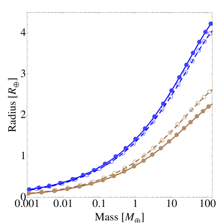
Figure 1: Mass-radius diagram showing the range of plausible phases for an atmosphere-less super-Earth (i.e. the boundary conditions), as derived from the model of Zeng & Sasselov (2013). Points taken from the model are shown as circles, along with our interpolation line shown overlaid. Blue is that of a 100%-H₂0 planet, blue-dashed is 75%-H₂0-25%-MgSiO₃, brown is 100%-Fe and brown-dashed is 75%-Fe-25%-MgSiO₃.

Table 1: Polynomial coefficients derived for the interpolation functions of the super-Earth mass-radius boundary conditions. Each column denotes a different composition, where we describe $(R_{P}/R_{\oplus})=\sum_{n=0}^{7}a_{n}[\log_{e}(M_{P}/M_{\oplus})]^{n}$.

Parameter	100%-H20	75%-H20-25%-MgSiO3	75%-Fe-25%-MgSiO3	100%-Fe
$a_{0}$	$+1.409\times 10^{+0}$	$+1.346\times 10^{+0}$	$+8.633\times 10^{-1}$	$+7.714\times 10^{-1}$
$a_{1}$	$+3.942\times 10^{-1}$	$+3.797\times 10^{-1}$	$+2.522\times 10^{-1}$	$+2.180\times 10^{-1}$
$a_{2}$	$+5.015\times 10^{-2}$	$+4.669\times 10^{-2}$	$+3.040\times 10^{-2}$	$+2.485\times 10^{-2}$
$a_{3}$	$+2.513\times 10^{-3}$	$+1.992\times 10^{-3}$	$+9.476\times 10^{-4}$	$+6.916\times 10^{-4}$
$a_{4}$	$-4.557\times 10^{-4}$	$-3.469\times 10^{-4}$	$-2.628\times 10^{-4}$	$-2.037\times 10^{-4}$
$a_{5}$	$-9.717\times 10^{-5}$	$-7.638\times 10^{-5}$	$-4.463\times 10^{-5}$	$-3.366\times 10^{-5}$
$a_{6}$	$-3.900\times 10^{-6}$	$-6.315\times 10^{-6}$	$-3.001\times 10^{-6}$	$-2.271\times 10^{-6}$
$a_{7}$	$+1.777\times 10^{-7}$	$-1.981\times 10^{-7}$	$-7.668\times 10^{-8}$	$-5.882\times 10^{-8}$

Table 2: Supported range of our interpolation model, based on the extrema of the models computed by Zeng & Sasselov (2013).

Parameter	100%-H20	75%-H20-25%-MgSiO3	75%-Fe-25%-MgSiO3	100%-Fe
$M_{P,\mathrm{min}}$ $[M_{\oplus}]$	$4.854\times 10^{-4}$	$6.197\times 10^{-5}$	$6.454\times 10^{-6}$	$6.144\times 10^{-6}$
$M_{P,\mathrm{max}}$ $[M_{\oplus}]$	$4.864\times 10^{+2}$	$3.393\times 10^{+2}$	$1.397\times 10^{+2}$	$1.321\times 10^{+2}$

2.3 Confidence of $R_{\mathrm{MAH}}>0$

Using Equation 1, one may compute the posterior distribution of $R_{P,\mathrm{H20}}$ and then $R_{\mathrm{MAH}}$. From this latter distribution, one may easily compute the confidence of the planet in question maintaining an atmosphere, under the model assumptions. This is done by evaluating the number of realizations which yield $R_{\mathrm{MAH}}>0$:

$$\mathrm{P}(R_{\mathrm{MAH}}>0)=\frac{\mathrm{\#}\,\,\mathrm{realizations}\,\,\mathrm{where}\,\,R_{\mathrm{MAH}}>0}{\mathrm{\#}\,\,\mathrm{realizations}\,\,\mathrm{total}}.$$ (3)

3 Examples

3.1 GJ 1214b

As a pedagogical example, we consider here perhaps the most well-characterized small exoplanet to date, GJ 1214b. Originally discovered by Charbonneau et al. (2009), this 2.8 $R_{\oplus}$ planet orbits a nearby M4.5 dwarf and consequently there exists a considerable literature of observations for this system, spanning transits, high resolution stellar spectra, radial velocities and parallaxes (Anglada-Escudé et al., 2013). The planet has also been studied extensively using transit spectroscopy in the quest to identify molecular absorption features (e.g. Bean et al. 2011; Désert et al. 2011; Berta et al. 2012).

Although the system continues to be intensively observed and thus the physical parameters of this system are likely to be refined in the near future, we provide here an applied example of the minimum atmospheric heigh (MAH) calculation to the planet GJ 1214b. The most recent and comprehensive attempt to derive self-consistent parameters for the planet and host star comes from Anglada-Escudé et al. (2013), who combined an updated trigonometric parallax, medium infrared spectroscopy, re-analysed HARPS radial velocities, the photometric catalogue and a suite of transit measurements in their analysis.

After obtaining the posterior joint probability distribution of the system parameters (personal communication), we computed $R_{\mathrm{MAH}}$ using Equation 1 for a sample of $10^{5}$ realizations drawn from the ensemble. For computing $R_{P,\mathrm{H20}}(M_{P})$, we assumed the boundary condition associated with a 75%-H₂0-25%-MgSiO₃ composition from Zeng & Sasselov (2013). Table 3 provides the results of our analysis.

We find that 97.2% (2.2 $\sigma$) of realizations yield an $M_{P}$-$R_{P}$ location inconsistent with a super-Earth planet lacking an atmosphere, as shown in Fig. 2 and 3. We note that using a 100%-H₂0 composition boundary condition slightly reduces this to 94.6%. The minimum atmospheric height (MAH) of GJ 1214b is found to be $R_{\mathrm{MAH}}=0.54_{-0.24}^{+0.21}$ $R_{\oplus}$ (quoting the median and $\pm 34.1$% quantiles), which translates to $19.7_{-7.9}^{+6.1}$% of the total planetary radius.

Rogers & Seager (2010) pointed out that the reported mass and radius (together with the quoted uncertainties) of GJ 1214b from Charbonneau et al. (2009) suggest that the object almost surely has a gas atmosphere layer. Here, we have quantified the credibility of this inference by using the full joint posterior probability density function for mass and radius. GJ 1214b has an equilibrium temperature in the vicinity of $\sim$400—550 K, depending on its Bond albedo. If the atmosphere is convective and nearly adiabatic from roughly the transit radius to the base of the gas envelope (at $R\approx 2.25R_{\oplus}$), then the adiabatic compression results in an extremely hot envelope base if the atmosphere is significantly heavier than an H/He composition. The observed featureless transit spectrum (Bean et al. 2010; Bean et al. 2011; Berta et al. 2012 — although note that Croll et al. 2011 found that the transit spectrum was not featureless) suggests either a high mean molecular weight atmosphere or, if the composition is H/He, a high cloud layer masking the features that would otherwise be seen due to the large scale height (Miller-Ricci et al., 2009). Our analysis cautions against drawing any definitive conclusions about chemical composition from a featureless spectrum for this planet, given the current joint posterior for mass and radius. The best-fitting mass and radius values do suggest (if the spectrum is featureless) that either clouds in an H/He atmosphere or a small scale height due to heavy composition (e.g., H₂O) prevent observable variations with wavelength in the transit radius; but, as is clear in Fig. 2, solutions requiring arbitrarily little atmosphere remain consistent with the radial velocity and transit data, if the bulk composition is fairly light (pure water or water+silicate).

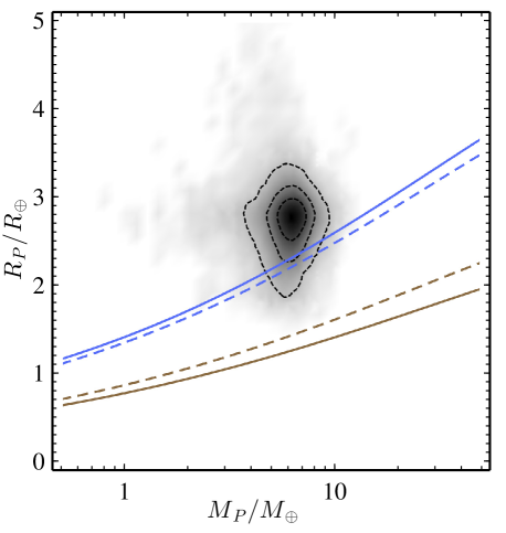
Figure 2: Zoomed-in version of Fig. 1 with the joint posterior distribution of GJ 1214b from Anglada-Escudé et al. (2013) shown overlaid. The three contours correspond to one, two and three-sigma confidence intervals. 97.2% (2.2 $\sigma$) of the points lie above the dashed blue line and thus are inconsistent with an atmosphere-less super-Earth.

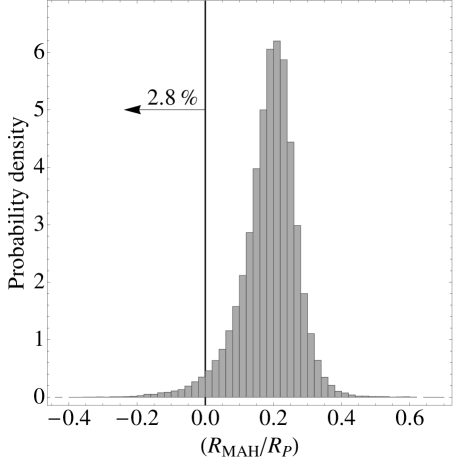
Figure 3: Marginalized posterior distribution of the minimum atmospheric height ($R_{\mathrm{MAH}}$) normalized by the planetary radius for GJ 1214b. Using the joint posteriors of Anglada-Escudé et al. (2013), the interior structure models of Zeng & Sasselov (2013) and Equation 1, we find $(R_{\mathrm{MAH}}/R_{P})=0.197_{-0.079}^{+0.061}$ and a 97.2% confidence that the planet maintains an extended atmosphere.

3.2 Other examples

We briefly comment that Neptune and Uranus both yield a positive $R_{\mathrm{MAH}}$, which is consistent with the estimate core-sizes of these worlds (see Table 3).

We also demonstrate the MAH calculation on four other exoplanet examples. KOI-142b is a planet detected by the transit technique and confirmed through transit timing variations (TTV) (Nesvorny et al., 2013) and is somewhat larger than that what might be typically associated with a “small” exoplanet. It is perhaps not surprising then that we find that the planet unambiguously has an atmosphere (posteriors obtained through personal communication).

Similarly, the planet Kepler-36c (Carter et al., 2012) has a radius close to that of Neptune but a lower mass and we find that every single posterior sample supports an extended atmosphere using $R_{\mathrm{MAH}}$. However, the other planet in the system, Kepler-36b, is significantly smaller at $\sim 1.5$ $R_{\oplus}$ with a mass of $\sim 4.5$ $M_{\oplus}$. In sharp contrast to Kepler-36c, we find every single posterior sample yields a negative $R_{\mathrm{MAH}}$. This planet is therefore an example of where the minimum atmospheric height method says nothing about whether this world does or does not have an atmosphere, as discussed earlier in §2.1.

Finally, we consider Kepler-22b which was detected by Borucki et al. (2012) and is similar in radius to GJ 1214b but lies in the habitable-zone of the host star. Determining whether the planet has a gaseous envelope or not is therefore particularly important due to the potential for habitability. The current radial velocity measurements for this system only place an upper limit on the planetary mass, limiting our ability to measure $R_{\mathrm{MAH}}$. Using posteriors from the recent re-analysis of Kipping et al. (2013), which includes more transit data, we find that planet straddles the boundary condition evenly and is consistent with either a water-world or water-world with a gas envelope.

Table 3: Example calculations of the minimum atmospheric height (MAH) for several planets. For Solar System planets we quote the equatorial radius and assume sphericity, as is done for exoplanets.

Planet	$M_{P}$ [$M_{\oplus}]$	$R_{P}$ [$R_{\oplus}]$	$\rho_{P}$ [g cm-3]	$R_{\mathrm{MAH}}$ [$R_{\oplus}]$	$(R_{\mathrm{MAH}}/R_{P})$	$\mathrm{P}(R_{\mathrm{MAH}}>0)$ [%]
GJ-1214b	$6.19_{-0.80}^{+0.80}$	$2.75_{-0.24}^{+0.18}$	$1.66_{-0.38}^{+0.56}$	$+0.54_{-0.24}^{+0.21}$	$+0.197_{-0.079}^{+0.061}$	$97.2$
KOI-142b	$6.6_{-6.1}^{+5.9}$	$4.23_{-0.39}^{+0.30}$	$0.48_{-0.45}^{+0.54}$	$+2.07_{-0.65}^{+1.00}$	$+0.47_{-0.12}^{+0.26}$	$>99.9$
Kepler-22b	$6.9_{-6.2}^{+20.9}$	$2.396_{-0.181}^{+0.088}$	$2.4_{-2.2}^{+7.5}$	$+0.11_{-0.87}^{+1.04}$	$+0.05_{-0.37}^{+0.44}$	$54.5$
Kepler-36b	$4.46_{-0.27}^{+0.34}$	$1.487_{-0.035}^{+0.034}$	$7.47_{-0.59}^{+0.72}$	$-0.537_{-0.047}^{+0.042}$	$-0.362_{-0.038}^{+0.034}$	$<0.01$
Kepler-36c	$8.09_{-0.45}^{+0.60}$	$3.682_{-0.056}^{+0.052}$	$0.891_{-0.045}^{+0.065}$	$+1.327_{-0.053}^{+0.049}$	$+0.361_{-0.012}^{+0.009}$	$>99.99$
Neptune	17.147	3.883	1.64	+1.08	+0.277	-
Uranus	14.536	4.007	1.27	+2.71	+0.325	-
Earth	1.000	1.000	5.52	-0.35	-0.350	-

4 Discussion

In this short paper, we have presented a simple, quantitative method to infer the minimum atmospheric height of an atmosphere (MAH) for an exoplanet using just a precise (and accurate) mass and radius measurement. In cases where the the $R_{\mathrm{MAH}}>0$ with high confidence, one infers the presence of an exoplanet atmosphere without ever taking a spectrum of the planet.

We envision that this metric will aid in the interpretation of exoplanet transit spectra by providing an additional boundary condition. For a given interior mass and radius ($M_{P}^{\rm int}$ and $R_{P}^{\rm int}$), and a given total mass and (transit) radius ($M_{P}$ and $R_{P}$), there are various possible atmospheric compositions. Imposing the constraint that the atmosphere should not be denser than the interior implies that some possible chemical compositions of the atmosphere are disallowed. Loosely speaking, one can think of a maximum mean molecular weight $\mu_{\rm max}$ for each possible “boundary condition” vector $\mathbf{B}=(M_{P}^{\rm int},R_{P}^{\rm int},M_{P},R_{P},T_{\rm eq})$, where $T_{\rm eq}$ is the atmospheric temperature at the transit radius. However, determining $\mu_{\rm max}[\mathbf{B}]$ would require a specific equation of state for each possible composition. In principle, the information in Fig. 2, for the example of GJ 1214b, is sufficient to allow for a calculation of $\mu_{\rm max}$, but this exercise is beyond the scope of this paper. But it seems clear that, as has been appreciated previously for GJ 1214b, light (H/He) and moderately heavy (e.g., H₂O) atmospheres are consistent with the data but, since the atmosphere appears to be $\sim$20% the radius of the planet, compositions much heavier than H₂O are disfavoured.

The simplicity and observationally “cheap” nature of determining $R_{\mathrm{MAH}}$ makes the metric attractive for general use within the exoplanet community. However, we do caution here that there are several limitations to appreciate when interpreting the minimum atmospheric height. Most importantly, the determination is fundamentally a model-dependent one, where in this work we used the models of Zeng & Sasselov (2013). Their model results rely on the most recent equations of states and experimental or theoretically determined properties of the bulk planetary materials. These will undoubtedly improve in the future and some dramatic surprises cannot be excluded, though appear unlikely. However, as far as our proposed method is concerned, it is trivial to replace this model with whatever mass-radius relation one prefers.

Considering the mass range of super-Earths, the boundary condition of a minimum contour of a pure-water planet, might still undergo significant correction in the planet models. Apart from the trivial uncertainty due to not knowing what is the maximum allowable water fraction (from formation and evolution), there is little understanding of the amount of mixing that could occur between a water and a H/He envelope (e.g. Nettelmann et al. 2011). It is likely that this occurs at a particular narrow range of pressures, and hence will be dependent on planetary mass, introducing additional structure in the mass-radius diagram.

Aside from aiding in the interpretation of exoplanetary spectra, our metric provides a quick and cost-effective method to assist in the selection and planning of follow-up atmospheric characterization for exoplanets. This is particularly important in light of the burgeoning catalogue of exoplanets and the upcoming planned missions for exoplanet characterization such as EChO (Tinetti et al., 2012). It should be trivial for observers to calculate $R_{\mathrm{MAH}}$ from their parameter posteriors (using Equation 1, Equation 2 and coefficients from Table 1) and thus provide a statistically meaningful statement regarding the presence of an extended atmosphere, which will surely aid in the selection and planning of follow-up observations.

References

- Agol et al. (2010) Agol, E., Cowan, N. B., Knutson, H. A., Deming, D., Steffen, J. H., Henry, G. W. & Charbonneau, D., 2010, ApJ, 721, 1861
- Anglada-Escudé et al. (2013) Anglada-Escudé, G., Rojas-Ayala, b., Boss, A. P., Weinberger, A. J. & Lloyd, J. P., 2013, A&A, 551, 48
- Batalha et al. (2013) Batalha, N. M. et al., 2013, ApJS, 204, 24
- Bean et al. (2010) Bean, J. L., Miller-Ricci Kempton, E., & Homeier, D. 2010, Nature, 468, 669
- Bean et al. (2011) Bean, J. L. et al., 2011, ApJ, 743, 92
- Benneke & Seager (2012) Benneke, B. & Seager, S., 2012, ApJ, 753, 100
- Berta et al. (2012) Berta, Z. K. et al., 2012, ApJ, 747, 35
- Borucki et al. (2012) Borucki, W. J. et al., ApJ, 745, 120
- Carter et al. (2012) Carter, J. A. et al., 2012, Science, 337, 667
- Charbonneau et al. (2002) Charbonneau, D., Brown, T. M., Noyes, R. W. & Gilliland, R. L., 2002, ApJ, 568, 377
- Charbonneau et al. (2009) Charbonneau, D. et al., 2009, Nature, 462, 891
- Croll et al. (2011) Croll, B., Albert, L., Jayawardhana, R., Miller-Ricci Kempton, E., Fortney, J. J., Murray, N., & Neilson, H. 2011, ApJ, 736, 78
- Désert et al. (2011) Désert, J.-M. et al., 2011, ApJ, 731, 40
- Dong & Zhu (2012) Dong, S. & Zhu, ApJ, submitted (astro-ph/1212.4853)
- Fraine et al. (2013) Fraine, J. D. et al., 2013, ApJ, 765, 127
- Fressin et al. (2013) Fressin, F. et al., 2013, ApJ, 766, 81
- Kipping et al. (2013) Kipping, D. et al., 2013, ApJ, submitted (astro-ph/1306.1530)
- Marcus et al. (2010) Marcus, R. A., Sasselov, D., Stewart, S. & Hernquist, L., 2010, ApJ, 719, 45
- Miller-Ricci et al. (2009) Miller-Ricci, E., Seager, S., & Sasselov, D. 2009, ApJ, 690, 1056
- Mordasini et al. (2009) Mordasini, C., Alibert, Y. & Benz, W., 2009, A&A, 501, 1139
- Nesvorny et al. (2013) Nesvorny, D. et al., 2013, ApJ, submitted (astro-ph/1304.4283)
- Nettelmann et al. (2011) Nettelmann, N., Fortney, J. J., Kramm, U. & Redmer, R., 2011, ApJ, 733, 2
- Pollack et al. (1996) Pollack, J. B., Hubickyj, O., Bodenheimer, P., Lissauer, J. J., Podolak, M., Greenzweig, Y., 1996, Icarus, 124, 62
- Schneider et al. (2011) Schneider J., Dedieu C., Le Sidaner P., Savalle R., Zolotukhin I., 2011, A&A, 532, A79
- Rogers & Seager (2010) Rogers, L. A. & Seager, S. 2010, ApJ, 716, 1208
- Seager & Deming (2010) Seager, S. & Deming, D., 2010, A&A, 48, 631
- Sing et al. (2012) Sing, D. K. et al., 2012, MNRAS, 426, 1663
- Tinetti et al. (2007) Tinetti, G. et al., 2007, Nature, 448, 169
- Tinetti & Beaulieu (2009) Tinetti, G. & Beaulieu, J. P., 2009, Proc. IAU Symposium No. 253, Queloz, D., Sasselov, D., Torres, M., & Holman, M., eds., p. 231
- Tinetti et al. (2012) Tinetti, G. et al., 2012, Exp. Astron., 34, 311
- Valencia et al. (2006) Valencia, D., O’Connell, R. & Sasselov, D., 2006, Icarus, 181, 545
- Zeng & Sasselov (2013) Zeng, L. & Sasselov, D., 2013, PASP, 125, 227
- Schneider et al. (2011) Schneider, J., Dedieu, C., Le Sidaner, P., Savalle, R., & Zolotukhin, I. 2011, A&A, 532, A79