Electrical control of phonon mediated spin relaxation rate in semiconductor quantum dots: the Rashba vs the Dresselhaus spin-orbit couplings

Abstract

In symmetric quantum dots (QDs), it is well known that the spin-hot spot (i.e., the cusp-like structure due to the presence of degeneracy near the level or anticrossing point) is present for the pure Rashba case but is absent for the pure Dresselhaus case [Phys. Rev. Lett. 95, 076805 (2005)]. Since the Dresselhaus spin-orbit coupling dominates over the Rashba spin-orbit coupling in GaAs and GaSb QDs, it is important to find the exact location of the spin-hot spot or the cusp-like structure even for the pure Dresselhaus case. In this paper, for the first time, we present analytical and numerical results that show that the spin-hot spot can also be seen for the pure Dresselhaus spin-orbit coupling case by inducing large anisotropy through external gates. At or nearby the spin-hot spot, the spin transition rate enhances and the decoherence time reduces by several orders of magnitude compared to the case with no spin-hot spot. Thus one should avoid such locations when designing QD spin based transistors for the possible implementation in quantum logic gates, solid state quantum computing and quantum information processing. It is also possible to extract the exact experimental data (Phys. Rev. Lett. 100, 046803 (2008)) for the phonon mediated spin-flip rates from our developed theoretical model.

I Introduction

Manipulation of a single electron spin with the application of gate controlled electric fields in a confined semiconductor QDs is a promising way for developing spin based quantum logic gates, spin memory devices for various quantum information processing applications. Loss and DiVincenzo (1998); Awschalom et al. (2002); Hanson et al. (2005); Kroutvar et al. (2004); Elzerman et al. (2004); Glazov et al. (2010); Climente et al. (2007); Pietiläinen and Chakraborty (2006); Chakraborty and Pietiläinen (2005); Nowak and Szafran (2011, 2009, 2010) Sufficiently short gate operation time combined with long decoherence time is one of the requirements for quantum computing. Golovach et al. (2004); Wang et al. (2011); Loss and DiVincenzo (1998) When a qubit is operated on by a classical bit, then its decay time is given by a spin relaxation time which is also supposed to be longer than the minimum time required to execute one quantum gate operation. Golovach et al. (2004); Awschalom et al. (2002); Amasha et al. (2008); Bandyopadhyay (2000); Fujisawa et al. (2001) Long spin relaxations have been measured experimentally in both symmetric and asymmetric QDs. Amasha et al. (2008); Elzerman et al. (2004); Kroutvar et al. (2004) Balocchi et. al. Balocchi et al. (2011) have recently measured larger spin relaxation times ($\mathrm{30~{}ns}$) in GaAs QDs. More specifically, both isotropic and anisotropic spin relaxations can be tuned with spin orbit coupling by choosing the growth direction parallel to the crystallographic axis [001], [110] and [111] of III-V zinc blend semiconductor QDs. Glazov et al. (2010); Balocchi et al. (2011); Griesbeck et al. (2012); Olendski and Shahbazyan (2007) In addition to the lengthening spin coherence time, the electric field tuning of spin relaxation forms the basis for turning the spin current on and off in some spin transistor proposals that can help to initialize electron spin based quantum computers. Bandyopadhyay (2000); Flatté (2011) These experimental studies confirm that the manipulation of spin-flip rates mediated by phonons due to spin-orbit coupling is an important ingredient for the design of robust spintronics logic devices. The spin-orbit coupling is mainly dominated by the Rashba Bychkov and Rashba (1984) and the linear Dresselhaus Dresselhaus (1955) terms in III-V semiconductor QDs. Prabhakar and Raynolds (2009); Prabhakar et al. (2010); de Sousa and Das Sarma (2003); Prabhakar et al. (2012); Folk et al. (2001); Fujisawa et al. (2001, 2002); Hanson et al. (2003); Pryor and Flatté (2006, 2007); Nowak et al. (2011) The Rashba spin-orbit coupling arises from structural inversion asymmetry along the growth direction while the Dresselhaus spin-orbit coupling arises from the bulk inversion asymmetry of the crystal lattice. Bychkov and Rashba (1984); Dresselhaus (1955)

In Ref. Bulaev and Loss, 2005a, b, the authors report that the cusp-like structure in the phonon mediated spin transition rate can be seen for the pure Rashba case. For the pure Dresselhaus case, the spin transition rate is a monotonous function of the magnetic fields and QDs radii. Since the Dresselhaus spin-orbit coupling dominates over the Rashba spin-orbit coupling in some materials such as GaAs and GaSb QDs, Prabhakar et al. (2010) it is important to find the exact location of spin-hot spot or the cusp-like structure even for the pure Dresselhaus case. The cusp like structure implies shorter spin relaxation and decoherence time which is hazardous for spin based applications such as quantum logic gates, solid state quantum computing and quantum information processing. For these applications, the spin-hot spot in the phonon mediated spin relaxation rate is something to avoid during the design of QD spin based transistors. Very recently, the authors in Ref. Yang et al., measured the spin-hot spot in the phonon mediated spin relaxation rate in Silicon QDs with the application of tuning very weak spin orbit coupling when Zeeman energy and valley splittings induce degeneracy. At the spin-hot spot in Silicon QDs, the dramatic rate enhancement decreases the decoherence time which is not supposed to be the ideal location for the qubit operation. Peng et al. (2013); Koh et al. (2012); Shi et al. (2012); Prance et al. (2012) In this paper, we obtain new analytical and numerical results for the behavior of the spin relaxation rate in anisotropic III-V semiconductor QDs. For the first time, we show the spin-hot spot in the phonon mediated spin transition rate can be seen for the pure Dresselhaus case by creating large anisotropy through external gates. Note that such location (spin-hot spot) is hazardous for quantum computing and quantum information processing, and must therefore be avoided during the design of spin based transistors.

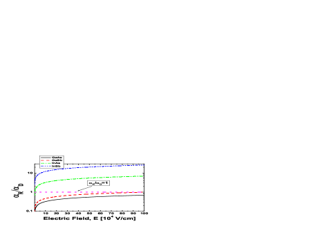
Figure 1: (Color online) Interplay between Rashba-Dresselhaus spin-orbit coupling vs the applied electric field along the z-direction. The Rashba spin-orbit coupling is seen to dominate in InAs and InSb QDs whereas the Dresselhaus spin-orbit coupling is seen to dominate in GaAs and GaSb QDs.

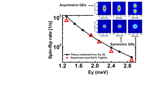
Figure 2: (Color online) Relaxation rate vs anisotropy in QDs. We choose $B=3~{}T$, $\ell_{0}=10~{}nm$, $\lambda_{R}=\lambda_{D}=1.7~{}\mu m$ and $a=5$. Here we define $\lambda_{R}=\hbar^{2}/m\alpha_{R}$, $\lambda_{D}=\hbar^{2}/m\alpha_{D}$, $E_{x}=\hbar\omega_{0}\sqrt{a}$ and $E_{y}=\hbar\omega_{0}\sqrt{b}$. The choice of these parameters mimics the experimentally reported values in Ref. Amasha et al., 2008. It can be seen that the theoretically obtained spin relaxation rate is in excellent agreement with the experimentally reported values in Ref. Amasha et al., 2008. For symmetric QDs, (lower panel, inset plot), we chose $a=b=5$.

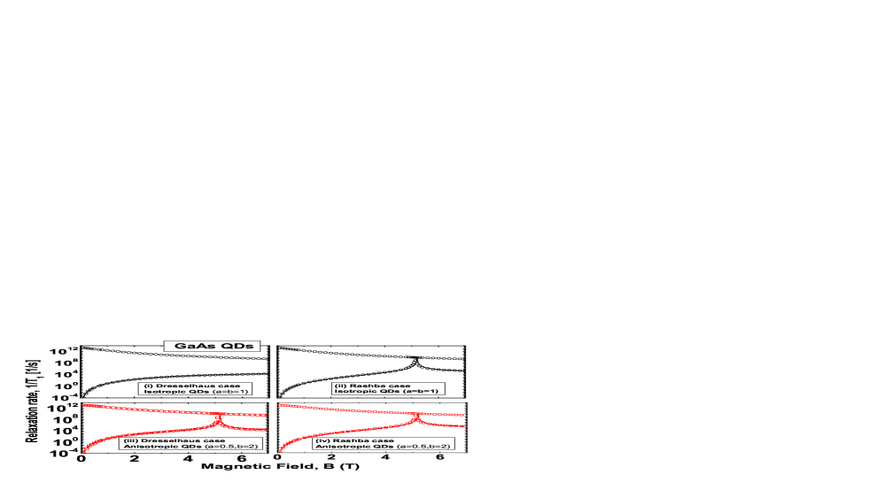
Figure 3: (Color online) Contributions of the Rashba and the Dresselhaus spin-orbit couplings to the phonon induced spin-flip rate as a function of magnetic fields. Material constants are chosen the same as in Fig. 1, but $\hbar\omega_{0}=1.1~{}meV$ and $\lambda_{R}=\lambda_{D}=8\mu m$. Solid lines (blue) are obtained from Eq. 17. Open circles and squares are obtained numerically from Eq. 16 by an exact diagonalization scheme implemented via Finite Element Method. com Notice that a cusp-like structure can be seen for the pure Dresselhaus case in asymmetric QDs (Fig. 2 (iii), $a\neq b$), but not for symmetric QDs (Fig. 2 (i), $a=b$). Also, the spin-flip rate vanishes like $B^{5}$ (see Eq. 25). Fig. 2(i) is Loss et. al. proposal for symmetric QDs (see Ref. Bulaev and Loss, 2005a). Fig. 2(iii) is our proposal for asymmetric QDs. We also expect a similar cusp-like structure for the pure Dresselhaus case with heavy holes in asymmetric QDs which is different from Ref. Bulaev and Loss, 2005a.

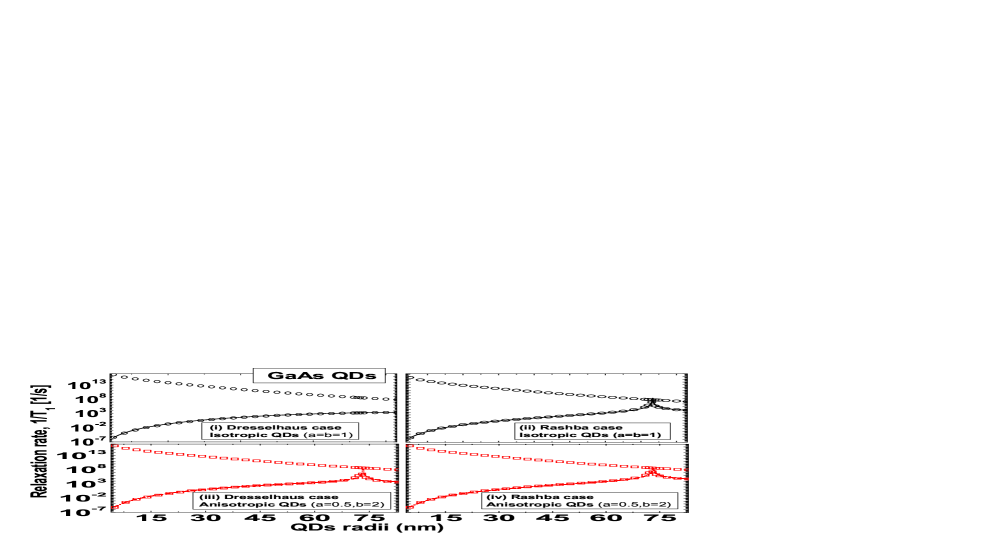
Figure 4: (Color online) Same as Fig. 2 but $1/T_{1}$ vs $\ell_{0}$. Here we chose, $B=1T$. Again, notice the cusp-like structure can only be seen for the pure Dresselhaus case in asymmetric QDs (Fig. 3 (iii), $a\neq b$) but not for symmetric QDs (Fig. 3 (i), $a=b$). Also, the spin-flip rate vanishes like $\ell_{0}^{8}$ (see Eq. 25).

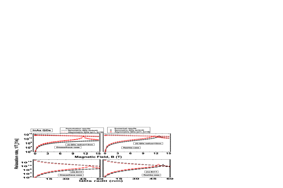
Figure 5: (Color online) Same as Figs. 2 and 3 but for InAs QDs. We chose $E=10^{5}~{}V/cm$. Again, notice the cusp-like structure can also be seen for the pure Dresselhaus case in asymmetric QDs $(a\neq b)$, but not for symmetric QDs $(a=b$).

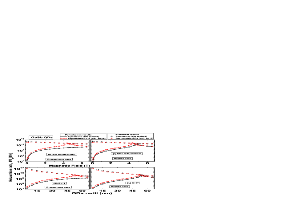
Figure 6: (Color online) Same as Fig. 2 and 3, but for GaSb QDs. We chose $E=10^{5}~{}V/cm$. Again, notice the cusp-like structure can also be seen for the pure Dresselhaus case in asymmetric QDs $(a\neq b)$, but not for symmetric QDs $(a=b$).

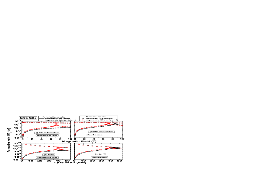
Figure 7: (Color online) Same as Fig. 2 and 3 but for InSb QDs. We chose $E=10^{4}~{}V/cm$. Again, notice the cusp-like structure can also be seen for the pure Dresselhaus case in asymmetric QDs $(a\neq b)$, but not for symmetric QDs $(a=b$).

The paper is organized as follows. In section II, we develop a theoretical model for anisotropic spin relaxation mediated by piezo-phonons that will allow us to investigate the interplay between the Rashba and the linear Dresselhaus spin-orbit couplings in QDs. In section III, we provide details of the diagonalization technique used for finding the energy spectrum and the matrix elements of the phonon mediated spin transition rate in QDs. In section IV, we plot both isotropic and anisotropic spin relaxation rates vs. magnetic fields and QDs radii for the pure Rashba and the pure Dresselhaus case in III-V semiconductor materials of zinc blend structure such as GaAs, GaSb, InAs and InSb. Finally, in section V, we summarize our results.

II Theoretical Model

We consider 2D anisotropic semiconductor QDs in the presence of a magnetic field along the growth direction. The total Hamiltonian of an electron in anisotropic QDs including spin-orbit interactions can be written as de Sousa and Das Sarma (2003); Khaetskii and Nazarov (2000); Bulaev and Loss (2005a) $H=H_{xy}+H_{so}$, where $H_{so}=H_{R}+H_{D}$ is the Hamiltonian associated with the Rashba-Dresselhaus spin-orbit couplings and $H_{xy}$ is the Hamiltonian of the electron in anisotropic QDs. $H_{xy}$ can be written as

$$H_{xy}={\frac{\vec{P}^{2}}{2m}}+{\frac{1}{2}}m\omega_{o}^{2}(ax^{2}+by^{2})+{\frac{1}{2}}g_{o}\mu_{B}\sigma_{z}B,$$ (1)

where $\vec{P}=\vec{p}+e\vec{A}$ is the kinetic momentum operator, $\vec{p}=-i\hbar(\partial_{x},\partial_{y},0)$ is the canonical momentum operator, $\vec{A}=B\left(-y\sqrt{b},x\sqrt{a},0\right)/\left(\sqrt{a}+\sqrt{b}\right)$ is the vector potential in the asymmetric gauge, $m$ is the effective mass, $\mu_{B}$ is the Bohr magneton, $\vec{\sigma}=\left(\sigma_{x},\sigma_{y},\sigma_{z}\right)$ are the Pauli spin matrices, $g_{0}$ is the bulk g-factor, $\omega_{0}=\hbar/(m\ell_{0}^{2})$ is the parabolic confining potential and $\ell_{0}$ is the radius of the QDs. The energy spectrum of $H_{xy}$ can be written as de Sousa and Das Sarma (2003); Prabhakar et al. (2011)

$$\varepsilon^{0}_{n_{+},n_{-},\pm}=\left(n_{+}+n_{-}+1\right)\hbar\omega_{+}+\left(n_{+}-n_{-}\right)\hbar\omega_{-}\pm\frac{\Delta}{2},\\$$ (2)

where $\omega_{\pm}=\frac{1}{2}\left[\omega_{c}^{2}+\omega_{0}^{2}\left(\sqrt{a}\pm\sqrt{b}\right)^{2}\right]^{1/2}$, $\Delta=g_{0}\mu_{B}B$ and $n_{\pm}$ are the eigenvalues of the Fock-Darwin number operators $a_{\pm}^{\dagger}a_{\pm}$. Here, $a_{\pm}$ and $a_{\pm}^{\dagger}$ are usual annihilation and creation operators. Also, we label the Fock-Darwin states as $|n_{+},n_{-},\pm\rangle$ with $\pm$ being the eigenvalues of the Pauli spin matrix along z-direction. de Sousa and Das Sarma (2003); Prabhakar and Raynolds (2009)

Finally, $H_{so}$ can be written as de Sousa and Das Sarma (2003)

$$H_{so}=\frac{\alpha_{R}}{\hbar}\left(\sigma_{x}P_{y}-\sigma_{y}P_{x}\right)+\frac{\alpha_{D}}{\hbar}\left(-\sigma_{x}P_{x}+\sigma_{y}P_{y}\right),$$ (3)

where

$$\alpha_{R}=\gamma_{R}eE,~{}~{}\alpha_{D}=0.78\gamma_{D}\left(\frac{2meE}{\hbar^{2}}\right)^{2/3}.$$ (4)

Here $\gamma_{R}$ and $\gamma_{D}$ are the Rashba and Dresselhaus spin-orbit coefficients. In Fig. 1, we have plotted the contribution of the Rashba-Dresselhaus spin-orbit coupling ($\alpha_{R}/\alpha_{D}$) with the variation of applied electric fields ($E$) along the z-direction. It can be seen that the Rashba spin-orbit coupling dominates in InAs and InSb QDs whereas the Dresselhaus spin-orbit coupling dominates in GaAs and GaSb QDs. In section IV we will focus our investigation on the phonon mediated spin-relaxation in both symmetric and asymmetric QDs.

The Hamiltonian (3) can be written in terms of raising and lowering operators as

$$H_{so} = \alpha_{R}\left(1+i\right)\left[b^{1/4}\kappa_{+}\left(s_{+}-i\right)a_{+}+b^{1/4}\kappa_{+}\left(s_{-}+i\right)a_{-}+a^{1/4}\eta_{-}\left(i-s_{-}\right)a_{+}+a^{1/4}\eta_{-}\left(i+s_{+}\right)a_{-}\right]$$ (5)

$$+\alpha_{D}\left(1+i\right)\left[a^{1/4}\kappa_{-}\left(i-s_{-}\right)a_{+}+a^{1/4}\kappa_{-}\left(i+s_{+}\right)a_{-}+b^{1/4}\eta_{+}\left(-i+s_{+}\right)a_{+}+b^{1/4}\eta_{+}\left(i+s_{-}\right)a_{-}\right]+H.c.,~{}~{}~{}~{}~{}~{}$$

where

$$s_{\pm}=\frac{\omega_{+}}{\omega_{c}\left(\frac{b}{a}\right)^{\frac{1}{4}}}\left[\sqrt{\frac{b}{a}}-1\pm\left[\frac{\omega_{c}^{2}\sqrt{\frac{b}{a}}}{\omega_{+}^{2}}+\left(1-\sqrt{\frac{b}{a}}\right)^{2}\right]^{\frac{1}{2}}\right],~{}~{}~{}$$ (6)

$$\kappa_{\pm}=\frac{1}{2\left(s_{+}-s_{-}\right)}\left\{\frac{1}{\ell}\sigma_{x}\pm i\frac{eB\ell}{\hbar}\left(\frac{1}{\sqrt{a}+\sqrt{b}}\right)\sigma_{y}\right\},~{}~{}~{}~{}$$ (7)

$$\eta_{\pm}=\frac{1}{2\left(s_{+}-s_{-}\right)}\left\{\frac{1}{\ell}\sigma_{y}\pm i\frac{eB\ell}{\hbar}\left(\frac{1}{\sqrt{a}+\sqrt{b}}\right)\sigma_{x}\right\},~{}~{}~{}~{}$$ (8)

H.c. represents the Hermitian conjugate, $\ell=\sqrt{\hbar/m\Omega}$ is the hybrid orbital length and $\Omega=\sqrt{\omega_{0}^{2}+\omega_{c}^{2}/\left(\sqrt{a}+\sqrt{b}\right)^{2}}$.

At low electric fields and small QDs radii, we treat the Hamiltonian associated with the Rashba and linear Dresselhaus spin-orbit couplings as a perturbation. Using second order non degenerate perturbation theory, the energy spectrum of the two lowest electron spin states in QDs (for details, see Ref. Prabhakar et al., 2011) is given by

$$\varepsilon_{0,0,+}=\hbar\varpi_{+}-\frac{\alpha_{R}^{2}\xi_{+}+\alpha_{D}^{2}\varsigma_{+}}{\hbar\omega_{x}-\Delta}-\frac{\alpha_{R}^{2}\varsigma_{-}+\alpha_{D}^{2}\xi_{-}}{\hbar\omega_{y}-\Delta},$$ (9)

$$\varepsilon_{0,0,-}=\hbar\varpi_{-}-\frac{\alpha_{R}^{2}\varsigma_{+}+\alpha_{D}^{2}\xi_{+}}{\hbar\omega_{x}+\Delta}-\frac{\alpha_{R}^{2}\xi_{-}+\alpha_{D}^{2}\varsigma_{-}}{\hbar\omega_{y}+\Delta},$$ (10)

where $\varpi_{\pm}=\omega_{+}\pm\omega_{z}/2$, $\omega_{z}=\Delta/\hbar$ is the Zeeman frequency, $\omega_{x}=\omega_{+}+\omega_{-}$, and $\omega_{y}=\omega_{+}-\omega_{-}$. Also,

$$\xi_{\pm}=\frac{1}{2(s_{+}-s_{-})}\left\{\pm\frac{1}{s_{\pm}}\alpha^{2}_{\pm}+2\alpha_{\pm}\beta_{\pm}\mp\frac{1}{s_{\mp}}\beta^{2}_{\pm}\right\},$$ (11)

$$\varsigma_{\pm}=\frac{1}{2(s_{+}-s_{-})}\left\{\pm\frac{1}{s_{\pm}}\alpha^{2}_{\mp}-2\alpha_{\mp}\beta_{\mp}\mp\frac{1}{s_{\mp}}\beta^{2}_{\mp}\right\},$$ (12)

$$\alpha_{\pm}=a^{1/4}\left\{\frac{1}{\ell}\pm\frac{eB\ell}{\hbar}\frac{1}{\left(\sqrt{a}+\sqrt{b}\right)}\right\},$$ (13)

$$\beta_{\pm}=b^{1/4}\left\{\frac{1}{\ell}\pm\frac{eB\ell}{\hbar}\frac{1}{\left(\sqrt{a}+\sqrt{b}\right)}\right\}.$$ (14)

We now turn to the calculation of the phonon induced spin relaxation rate at absolute zero temperature between two lowest energy states in QDs. Following Ref. Prabhakar et al., 2012; de Sousa and Das Sarma, 2003; Khaetskii and Nazarov, 2000, 2001, the interaction between electron and piezo-phonon can be written Gantmakher and Levinson (1987)

$$u^{\mathbf{q}\alpha}_{ph}\left(\mathbf{r},t\right)=\sqrt{\frac{\hbar}{2\rho V\omega_{\mathbf{q}\alpha}}}e^{i\left(\mathbf{q\cdot r}-\omega_{q\alpha}t\right)}eA_{\mathbf{q}\alpha}b^{{\dagger}}_{\mathbf{q}\alpha}+H.c.,$$ (15)

where $\rho$ is the crystal mass density and $V$ is the volume of the QD. $b^{{\dagger}}_{\mathbf{q}\alpha}$ creates an acoustic phonon with wave vector $\mathbf{q}$ and polarization $\hat{e}_{\alpha}$, where $\alpha=l,t_{1},t_{2}$ are chosen as one longitudinal and two transverse modes of the induced phonon in the dots. $A_{\mathbf{q}\alpha}=\hat{q}_{i}\hat{q}_{k}e\beta_{ijk}e^{j}_{\mathbf{q}\alpha}$ is the amplitude of the electric field created by phonon strain, where $\hat{\mathbf{q}}=\mathbf{q}/q$ and $e\beta_{ijk}=eh_{14}$ for $i\neq k,i\neq j,j\neq k$. The polarization directions of the induced phonon are $\hat{e}_{l}=\left(\sin\theta\cos\phi,\sin\theta\sin\phi,\cos\theta\right)$, $\hat{e}_{t_{1}}=\left(\cos\theta\cos\phi,\cos\theta\sin\phi,-\sin\theta\right)$ and $\hat{e}_{t_{2}}=\left(-\sin\phi,\cos\phi,0\right)$. Based on the Fermi Golden Rule, the phonon induced spin transition rate in the QDs is given by de Sousa and Das Sarma (2003); Khaetskii and Nazarov (2001)

$$\frac{1}{T_{1}}=\frac{2\pi}{\hbar}\int\frac{d^{3}\mathbf{q}}{\left(2\pi\right)^{3}}\sum_{\alpha=l,t}\arrowvert M\left(\mathbf{q}\alpha\right)\arrowvert^{2}\delta\left(\hbar s_{\alpha}\mathbf{q}-\varepsilon_{f}+\varepsilon_{i}\right),$$ (16)

where $s_{l}$,$s_{t}$ are the longitudinal and transverse acoustic phonon velocities in QDs. The matrix element $M\left(\mathbf{q}\alpha\right)=\langle\psi_{i}|u^{\mathbf{q}\alpha}_{ph}\left(\mathbf{r},t\right)|\psi_{f}\rangle$ with the emission of one phonon $\mathbf{q}\alpha$ has been calculated perturbatively and numerically. Khaetskii and Nazarov (2001); Stano and Fabian (2006); com Here $|\psi_{i}\rangle$ and $|\psi_{f}\rangle$ correspond to the initial and finial states of the Hamiltonian $H$. Based on second order non degenerate perturbation theory, after long algebraic tranformations, we have:

$$\frac{1}{T_{1}}=c\left(|M_{x}|^{2}+|M_{y}|^{2}\right),$$ (17)

where

$$c=\frac{2\left(eh_{14}\right)^{2}\left(g\mu_{B}B\right)^{3}}{35\pi\hbar^{4}\rho}\left(\frac{1}{s^{5}_{l}}+\frac{4}{3}\frac{1}{s^{5}_{t}}\right),~{}~{}~{}~{}~{}~{}~{}$$ (18)

$$M_{x}=\frac{\left(is_{-}+1\right)\Xi_{1}\left(\hbar\omega_{x}+\Delta\right)+\left(-is_{-}+1\right)\Xi_{3}\left(\hbar\omega_{x}-\Delta\right)}{a^{1/4}\left[\left(\hbar\omega_{x}\right)^{2}-\Delta^{2}\right]}$$

$$+\frac{\left(-is_{+}+1\right)\Xi_{2}\left(\hbar\omega_{y}+\Delta\right)+\left(is_{+}+1\right)\Xi_{4}\left(\hbar\omega_{y}-\Delta\right)}{a^{1/4}\left[\left(\hbar\omega_{y}\right)^{2}-\Delta^{2}\right]},~{}~{}~{}~{}~{}~{}~{}$$ (19)

$$M_{y}=\frac{\left(is_{+}+1\right)\Xi_{1}\left(\hbar\omega_{x}+\Delta\right)+\left(-is_{+}+1\right)\Xi_{3}\left(\hbar\omega_{x}-\Delta\right)}{b^{1/4}\left[\left(\hbar\omega_{x}\right)^{2}-\Delta^{2}\right]}$$

$$+\frac{\left(is_{-}-1\right)\Xi_{2}\left(\hbar\omega_{y}+\Delta\right)+\left(-is_{-}-1\right)\Xi_{4}\left(\hbar\omega_{y}-\Delta\right)}{b^{1/4}\left[\left(\hbar\omega_{y}\right)^{2}-\Delta^{2}\right]},~{}~{}~{}~{}~{}~{}$$ (20)

$$\Xi_{1}=\frac{\ell}{2\left(s_{+}-s_{-}\right)^{2}}\left[\alpha_{R}\left\{\left(s_{+}+i\right)\beta_{+}+\left(1-is_{-}\right)\alpha_{+}\right\}+\alpha_{D}\left\{\left(-s_{-}-i\right)\alpha_{-}+\left(-1+is_{+}\right)\beta_{-}\right\}\right],~{}~{}~{}~{}$$ (21)

$$\Xi_{2}=\frac{\ell}{2\left(s_{+}-s_{-}\right)^{2}}\left[\alpha_{R}\left\{\left(s_{-}-i\right)\beta_{+}+\left(1+is_{+}\right)\alpha_{+}\right\}+\alpha_{D}\left\{\left(s_{+}-i\right)\alpha_{-}+\left(1+is_{-}\right)\beta_{-}\right\}\right],~{}~{}~{}~{}$$ (22)

$$\Xi_{3}=\frac{\ell}{2\left(s_{+}-s_{-}\right)^{2}}\left[\alpha_{R}\left\{\left(s_{+}-i\right)\beta_{-}+\left(-1-is_{-}\right)\alpha_{-}\right\}+\alpha_{D}\left\{\left(-s_{-}+i\right)\alpha_{+}+\left(1+is_{+}\right)\beta_{+}\right\}\right],~{}~{}~{}~{}$$ (23)

$$\Xi_{4}=\frac{\ell}{2\left(s_{+}-s_{-}\right)^{2}}\left[\alpha_{R}\left\{\left(s_{-}+i\right)\beta_{-}+\left(-1+is_{+}\right)\alpha_{-}\right\}+\alpha_{D}\left\{\left(s_{+}+i\right)\alpha_{+}+\left(-1+is_{-}\right)\beta_{+}\right\}\right].~{}~{}~{}~{}$$ (24)

In the above expression, we use $c=c_{l}I_{xl}+2c_{t}I_{xt}$, where $c_{\alpha}=\frac{q^{2}e^{2}}{\left(2\pi\right)^{2}\hbar^{2}s_{\alpha}}|\varepsilon_{q\alpha}|^{2}$, $|\varepsilon_{q\alpha}|^{2}=\frac{q^{2}\hbar}{2\rho\omega_{q\alpha}}$ and $q=\frac{g\mu_{B}B}{\hbar s_{\alpha}}$. Also, $g=\frac{\varepsilon_{0,0,-}-\varepsilon_{0,0,+}}{\mu_{B}B}$ is the Land$\acute{e}$ $g$-factor. For longitudinal phonon modes, Khaetskii and Nazarov (2001); Golovach et al. (2004) we have $|A_{q,l}|^{2}=36h_{14}^{2}\cos^{2}\theta\sin^{4}\theta\sin^{2}\phi\cos^{2}\phi$ and thus we find $I_{xl}=16\pi h^{2}_{14}/35$. For transverse phonon modes, we have $|A_{q,t}|^{2}=2h_{14}^{2}\left[\cos^{2}\theta\sin^{2}\theta+\sin^{4}\theta\left(1-9\cos^{2}\theta\right)\sin^{2}\phi\cos^{2}\phi\right]$ and thus we find $I_{xt}=32\pi h^{2}_{14}/105$.

For isotropic QDs ($a=b=1$, $s_{+}=1$ and $s_{-}=-1$), the spin relaxation rate is given by

$$\frac{1}{T_{1}}=\frac{2\left(eh_{14}\right)^{2}\left(g\mu_{B}B\right)^{3}}{35\pi\hbar^{4}\rho}\left(\frac{1}{s^{5}_{l}}+\frac{4}{3}\frac{1}{s^{5}_{t}}\right)\left(|M_{R}|^{2}+|M_{D}|^{2}\right),$$ (25)

where $M_{R}$ and $M_{D}$ are the coefficients of matrix elements associated with the Rashba and Dresselhaus spin-orbit couplings in QDs and are given by

$$M_{R}=\frac{\alpha_{R}}{\sqrt{2}\hbar\Omega}\left[\frac{1}{1-\frac{\Delta}{\hbar\left(\Omega+\frac{\omega_{c}}{2}\right)}}-\frac{1}{1+\frac{\Delta}{\hbar\left(\Omega-\frac{\omega_{c}}{2}\right)}}\right],$$ (26)

$$M_{D}=\frac{\alpha_{D}}{\sqrt{2}\hbar\Omega}\left[\frac{1}{1+\frac{\Delta}{\hbar\left(\Omega+\frac{\omega_{c}}{2}\right)}}-\frac{1}{1-\frac{\Delta}{\hbar\left(\Omega-\frac{\omega_{c}}{2}\right)}}\right].$$ (27)

Since $\Delta=g_{0}\mu_{B}B$ is negative for GaAs and InAs QDs, we see the degeneracy only appears in the Rashba case (see the 2nd term of Eq. 26) and the degeneracy is absent in the Dresselhaus case. The degeneracy in the Rashba case induces the level crossing point and cusp-like structure in the spin-flip rate in QDs. The spin relaxation rate for isotropic QDs can be written in a more convenient form as

$$\frac{1}{T_{1}} = \frac{2\left(eh_{14}\right)^{2}\left(g\mu_{B}B\right)^{3}}{35\pi\hbar^{4}\rho}\left(\frac{1}{s^{5}_{l}}+\frac{4}{3}\frac{1}{s^{5}_{t}}\right)\frac{2\Delta^{2}m^{4}}{\hbar^{8}}$$ (28)

$$\left(\alpha_{R}^{2}+\alpha_{D}^{2}\right)\ell_{0}^{8}\left[1+O\left(\omega_{c}/\omega_{o}\right)^{2}\right].$$

From Eq. 28, it is clear that the spin-flip rate vanishes like $B^{5}$ and $\ell_{0}^{8}$ (see Ref. de Sousa and Das Sarma, 2003).

Table 1: The material constants used in our calculations are taken from Refs. Cardona et al., 1988; de Sousa and Das Sarma, 2003

Parameters	GaAs	InAs	$GaSb$	InSb
$g_{0}$	-0.44	-15	$-7.8$	-50.6
m	0.067	0.0239	$0.0412$	0.0136
$\gamma_{R}~{}[{\AA}^{2}]$	4.4	110	$33$	500
$\gamma_{D}~{}[eV{\AA}^{3}]$	26	130	$187$	228
$eh_{14}~{}[10^{-5}erg/cm]$	2.34	0.54	$1.5$	0.75
$s_{l}~{}[10^{5}cm/s]$	5.14	4.2	$4.3$	3.69
$s_{t}~{}[10^{5}cm/s]$	3.03	2.35	$2.49$	2.29
$\rho~{}[g/cm^{3}]$	5.3176	5.667	$5.6137$	5.7747

III Computational Method

We suppose that a QD is formed at the center of a $400\times 400~{}\mathrm{nm^{2}}$ geometry. Then we diagonalize the total Hamiltonian $H$ numerically using the Finite Element Method. com The geometry contains $24910$ elements. Since the geometry is much larger compared to the actual lateral size of the QD, we impose Dirichlet boundary conditions, find the eigenvalues, eigenfunctions and the matrix elements $M\left(\mathbf{q}\alpha\right)$ of the total Hamiltonian $H$. From Figs. 2 to  7, the analytically obtained spin-flip rates from Eq. 17 (solid and dashed-dotted lines) are seen to be in excellent agreement with the numerical values (open circles and squares). The material constants are taken from table 1.

IV Results and Discussions

In Fig. 2, we compare theoretically obtained spin-flip rates from Eq. 17 to the experimentally reported values in Ref. Amasha et al., 2008. Theoretical and experimental data are in excellent agreement. Inset plots (from left to right) show realistic in-plane wavefunctions of QDs for the spin states $|0,0,+1/2\rangle$, $|0,0,-1/2\rangle$ and $|0,1,+1/2\rangle$. It can be seen that anisotropy breaks the in-plane rotational symmetry. As a result, we find that the in-plane wavefunction of anisotropic QDs for the states $|0,1,+1/2\rangle$ split into two which has a direct consequence on inducing accidental degeneracy even for the pure Dresselhaus spin-orbit coupling case in the phonon mediated spin flip rate. This will be separately discussed from Figs. 3 to 7.

In Fig. 3 (i) we see that the cusp-like structure is absent (i.e., the spin-flip rate is a monotonous function of the magnetic field) for the pure Dresselhaus case in symmetric QDs. However in Fig. 3(iii) we see that the cusp-like structure is present for the pure Dresselhaus case in asymmetric QDs. In Fig. 4, again we see that the cusp-like structure is absent in isotropic QDs ($a=b$) but is present in anisotropic QDs ($a\neq b$) for the pure Dresselhaus case. The cusp-like structure in anisotropic QDs is thus due to the fact that the anisotropy induces the accidental degeneracy in the matrix elements ($M\left(\mathbf{q}\alpha\right)$) near the level crossing or anticrossing point. The accidental degeneracy point where the cusp-like structure appears is referred to as the spin-hot spot while tuning on the spin-orbit coupling removes the degeneracy. Stano and Fabian (2006) Thus, we apply degenerate perturbation theory and the energy spectrum of the unperturbed spin states $|0,0,-\rangle$ and $|0,1,+\rangle$ for anisotropic QDs are given by

$$\varepsilon^{0}_{0,0,-}=\frac{3}{2}\hbar\omega_{+}-\frac{1}{2}\hbar\omega_{-}+\left[\alpha_{R}^{2}\xi_{-}+\alpha_{D}^{2}\zeta_{-}\right]^{1/2},$$ (29)

$$\varepsilon^{0}_{0,1,+}=\frac{3}{2}\hbar\omega_{+}-\frac{1}{2}\hbar\omega_{-}-\left[\alpha_{R}^{2}\xi_{-}+\alpha_{D}^{2}\zeta_{-}\right]^{1/2}.$$ (30)

We have substituted Eqs. 29 and 30 into 17 and found the spin-flip rate at the level crossing point from Figs. 2 to 7. Lifting the degeneracy with the application of spin-orbit couplings mixes spin up and spin down states where the phonon mediated spin transition rate between states of opposite magnetic moment will involve spin flips with a much more enhanced probability compared to the normal states. For example, the spin-hot spot for the pure Dresselhaus case in symmetric GaAs QDs (Figs. 3 (i) and  4 (i)) can not be observed while tuning the anisotropy ($a\neq b$), however can be observed at $B=5.1~{}T$ and $\ell_{0}=69~{}nm$ as shown in Figs. 3 (iii) and  4 (iii), respectively. Notice that the spin-flip rates of the pure Dresselhaus case found near the spin-hot spot in Figs. 3 (iii) and  4 (iii) are $6$ orders of magnitude larger than those values found in Figs. 3 (i) and 4(i). This result (i.e., the spin-hot spot in asymmetric QDs for the pure Dresselhaus case yet to be experimentally verified) provides small relaxation and decoherence time which should be avoided during the design of spin based transistors for the possible implementation in quantum logic gates, quantum computing and quantum information processing. From Figs. 4 to 7, we investigated the spin relaxation rate in InAs, GaSb and InSb QDs. Analyzing all plots, the spin-hot spot and associated cusp-like structure can be seen in the pure Dresselhaus spin-orbit coupling case in anisotropic QDs ($a\neq b$).

V Conclusions

We have shown that the anisotropy breaks the in-plane rotational symmetry. As a result, we found that the cusp-like structure (i.e., where the spin-hot spot) is present in the phonon mediated spin transition rate in anisotropic QDs for the pure Dresselhaus spin-orbit coupling case. In contrast, for isotropic QDs, the spin transition rate is a monotonous function of magnetic fields and QDs radii (i.e., where the spin-hot spot is absent) for the pure Dresselhaus spin-orbit coupling case. These results (yet to be experimentally verified) provide new information for finding the spin hot-spot in anisotropic spin relaxation for the pure Dresselhaus case during the design of QD spin transistors. At or nearby the spin-hot spot, the relaxation and decoherence time are smaller by several orders of magnitude. One should avoid such locations during the design of QD spin based transistors for the possible implementation in quantum logic gates, quantum computing and quantum information processing.

VI Acknowledgements

This work has been supported by Natural Science and Engineering Research Council (Canada) and Canada Research Chair programs. The authors acknowledge the Shared Hierarchical Academic Research Computing Network (SHARCNET) community and Dr. Philip James Douglas Roberts for the helpful and technical support.

References

- Loss and DiVincenzo (1998) D. Loss and D. P. DiVincenzo, Phys. Rev. A 57, 120 (1998).
- Awschalom et al. (2002) D. D. Awschalom, D. Loss, and N. Samarth, Semiconductor Spintronics and Quantum Computation (Springer, Berlin, 2002).
- Hanson et al. (2005) R. Hanson, L. H. W. van Beveren, I. T. Vink, J. M. Elzerman, W. J. M. Naber, F. H. L. Koppens, L. P. Kouwenhoven, and L. M. K. Vandersypen, Phys. Rev. Lett. 94, 196802 (2005).
- Kroutvar et al. (2004) M. Kroutvar, Y. Ducommun, D. Heiss, M. Bichler, D. Schuh, G. Abstreiter, and J. J. Finley, Nature 432, 81 (2004).
- Elzerman et al. (2004) J. M. Elzerman, R. Hanson, L. H. Willems van Beveren, B. Witkamp, L. M. K. Vandersypen, and L. P. Kouwenhoven, Nature 430, 431 (2004).
- Glazov et al. (2010) M. Glazov, E. Sherman, and V. Dugaev, Physica E: Low-dimensional Systems and Nanostructures 42, 2157 (2010).
- Climente et al. (2007) J. I. Climente, A. Bertoni, G. Goldoni, M. Rontani, and E. Molinari, Phys. Rev. B 75, 081303 (2007).
- Pietiläinen and Chakraborty (2006) P. Pietiläinen and T. Chakraborty, Phys. Rev. B 73, 155315 (2006).
- Chakraborty and Pietiläinen (2005) T. Chakraborty and P. Pietiläinen, Phys. Rev. Lett. 95, 136603 (2005).
- Nowak and Szafran (2011) M. P. Nowak and B. Szafran, Phys. Rev. B 83, 035315 (2011).
- Nowak and Szafran (2009) M. P. Nowak and B. Szafran, Phys. Rev. B 80, 195319 (2009).
- Nowak and Szafran (2010) M. P. Nowak and B. Szafran, Phys. Rev. B 81, 235311 (2010).
- Golovach et al. (2004) V. N. Golovach, A. Khaetskii, and D. Loss, Phys. Rev. Lett. 93, 016601 (2004).
- Wang et al. (2011) X. Wang, L. S. Bishop, J. Kestner, E. Barnes, K. Sun, and S. Das Sarma, Nat Commun 3, 997 (2011).
- Amasha et al. (2008) S. Amasha, K. MacLean, I. P. Radu, D. M. Zumbühl, M. A. Kastner, M. P. Hanson, and A. C. Gossard, Phys. Rev. Lett. 100, 046803 (2008).
- Bandyopadhyay (2000) S. Bandyopadhyay, Phys. Rev. B 61, 13813 (2000).
- Fujisawa et al. (2001) T. Fujisawa, Y. Tokura, and Y. Hirayama, Phys. Rev. B 63, 081304 (2001).
- Balocchi et al. (2011) A. Balocchi, Q. H. Duong, P. Renucci, B. L. Liu, C. Fontaine, T. Amand, D. Lagarde, and X. Marie, Phys. Rev. Lett. 107, 136604 (2011).
- Griesbeck et al. (2012) M. Griesbeck, M. M. Glazov, E. Y. Sherman, D. Schuh, W. Wegscheider, C. Schüller, and T. Korn, Phys. Rev. B 85, 085313 (2012).
- Olendski and Shahbazyan (2007) O. Olendski and T. V. Shahbazyan, Phys. Rev. B 75, 041306 (2007).
- Flatté (2011) M. E. Flatté, Physics 4, 73 (2011).
- Bychkov and Rashba (1984) Y. A. Bychkov and E. I. Rashba, J. Phys. C: Solid State Phys. 17, 6039 (1984).
- Dresselhaus (1955) G. Dresselhaus, Phys. Rev. 100, 580 (1955).
- Prabhakar and Raynolds (2009) S. Prabhakar and J. E. Raynolds, Phys. Rev. B 79, 195307 (2009).
- Prabhakar et al. (2010) S. Prabhakar, J. Raynolds, A. Inomata, and R. Melnik, Phys. Rev. B 82, 195306 (2010).
- de Sousa and Das Sarma (2003) R. de Sousa and S. Das Sarma, Phys. Rev. B 68, 155330 (2003).
- Prabhakar et al. (2012) S. Prabhakar, R. V. N. Melnik, and L. L. Bonilla, Applied Physics Letters 100, 023108 (2012).
- Folk et al. (2001) J. A. Folk, S. R. Patel, K. M. Birnbaum, C. M. Marcus, C. I. Duruöz, and J. S. Harris, Phys. Rev. Lett. 86, 2102 (2001).
- Fujisawa et al. (2002) T. Fujisawa, D. G. Austing, Y. Tokura, Y. Hirayama, and S. Tarucha, Nature 419, 278 (2002).
- Hanson et al. (2003) R. Hanson, B. Witkamp, L. M. K. Vandersypen, L. H. W. van Beveren, J. M. Elzerman, and L. P. Kouwenhoven, Phys. Rev. Lett. 91, 196802 (2003).
- Pryor and Flatté (2006) C. E. Pryor and M. E. Flatté, Phys. Rev. Lett. 96, 026804 (2006).
- Pryor and Flatté (2007) C. E. Pryor and M. E. Flatté, Phys. Rev. Lett. 99, 179901 (2007).
- Nowak et al. (2011) M. P. Nowak, B. Szafran, F. M. Peeters, B. Partoens, and W. J. Pasek, Phys. Rev. B 83, 245324 (2011).
- Bulaev and Loss (2005a) D. V. Bulaev and D. Loss, Phys. Rev. Lett. 95, 076805 (2005a).
- Bulaev and Loss (2005b) D. V. Bulaev and D. Loss, Phys. Rev. B 71, 205324 (2005b).
- (36) C. Yang, A. Rossi, R. Ruskov, N. Lai, F. Mohiyaddin, S. Lee, C. Tahan, G. Klimeck, A. Morello, and A. Dzurak, arXiv:1302.0983 .
- Peng et al. (2013) W. Peng, Z. Aksamija, S. A. Scott, J. J. Endres, D. E. Savage, I. Knezevic, M. A. Eriksson, and M. G. Lagally, Nat Commun 4, 1339 (2013).
- Koh et al. (2012) T. S. Koh, J. K. Gamble, M. Friesen, M. A. Eriksson, and S. N. Coppersmith, Phys. Rev. Lett. 109, 250503 (2012).
- Shi et al. (2012) Z. Shi, C. B. Simmons, J. R. Prance, J. K. Gamble, T. S. Koh, Y.-P. Shim, X. Hu, D. E. Savage, M. G. Lagally, M. A. Eriksson, M. Friesen, and S. N. Coppersmith, Phys. Rev. Lett. 108, 140503 (2012).
- Prance et al. (2012) J. R. Prance, Z. Shi, C. B. Simmons, D. E. Savage, M. G. Lagally, L. R. Schreiber, L. M. K. Vandersypen, M. Friesen, R. Joynt, S. N. Coppersmith, and M. A. Eriksson, Phys. Rev. Lett. 108, 046808 (2012).
- (41) Comsol Multiphysics version 3.5a (www.comsol.com).
- Khaetskii and Nazarov (2000) A. V. Khaetskii and Y. V. Nazarov, Phys. Rev. B 61, 12639 (2000).
- Prabhakar et al. (2011) S. Prabhakar, J. E. Raynolds, and R. Melnik, Phys. Rev. B 84, 155208 (2011).
- Khaetskii and Nazarov (2001) A. V. Khaetskii and Y. V. Nazarov, Phys. Rev. B 64, 125316 (2001).
- Gantmakher and Levinson (1987) V. F. Gantmakher and Y. B. Levinson, Carrier Scattering in Metals and Semiconductor (North-Holland, Amsterdam, 1987).
- Stano and Fabian (2006) P. Stano and J. Fabian, Phys. Rev. B 74, 045320 (2006).
- Cardona et al. (1988) M. Cardona, N. E. Christensen, and G. Fasol, Phys. Rev. B 38, 1806 (1988).