A convenient implementation of the overlap between arbitrary Hartree-Fock-Bogoliubov vacua for projection

Abstract

Overlap between Hartree-Fock-Bogoliubov(HFB) vacua is very important in the beyond mean-field calculations. However, in the HFB transformation, the $U,V$ matrices are sometimes singular due to the exact emptiness ($v_{i}=0$) or full occupation ($u_{i}=0$) of some single-particle orbits. This singularity may cause some problem in evaluating the overlap between HFB vacua through Pfaffian. We found that this problem can be well avoided by setting those zero occupation numbers $u_{i},v_{i}$ to some tiny values denoted by $\varepsilon(>0)$, which numerically satisfies $1+\varepsilon^{2}=1$ (e.g., $\varepsilon=10^{-8}$ when using the double precision data type). This treatment does not change the HFB vacuum state because $u_{i}^{2},v_{i}^{2}=\varepsilon^{2}$ are numerically zero relative to 1. Therefore, for arbitrary HFB transformation, we say that the $U,V$ matrices can always be nonsingular. From this standpoint, we present a new convenient Pfaffian formula for the overlap between arbitrary HFB vacua, which is especially suitable for symmetry restoration. Testing calculations have been performed for this new formula. It turns out that our method is reliable and accurate in evaluating the overlap between arbitrary HFB vacua.

1 Introduction

The Hartree-Fock-Bogoliubov (HFB) approximation has been a great success in understanding interacting many-body quantum systems in all fields of physics. However, the beyond mean-field effects (e.g., the nuclear vibration and rotation) are missing in the HFB calculations. Methods that go beyond mean-field, such as the Generator Coordinate Method(GCM) and the projection method, are expected to take those missing effects into consideration and present better description of the many-body quantum system. In the beyond mean-field calculations, operator matrix elements and overlaps between multi-quasiparticle HFB states are basic blocks. These matrix elements and overlaps can be evaluated using the generalized Wick’s theorem (GWT)[1, 2], or equivalently using Pfaffian [3, 4, 5, 6, 7], or using the compact formula in Ref.[8]. However, in the efficient calculations (e.g., see [5]), all of the matrix elements and overlaps require the value of the overlap between HFB vacua.

Thus, the reliable and accurate evaluation of the overlap between HFB vacua is very important for the stability and the efficiency of the beyond mean-field calculations. Especially in cases near to the Egido pole [9], the overlap between HFB vacua is very tiny, and a small error could lead to a large uncertainty of the matrix elements. In the past, numerical calculations of the overlap were performed with the Onishi formula [10]. Unfortunately, the Onishi formula leaves the sign of the overlap undefined due to the square root of a determinant. Several efforts have been made to overcome this sign problem [11, 12, 13, 14, 15, 16]. In 2009, Robledo proposed a different overlap formula with the Pfaffian rather than the determinant [17]. This formula completely solves the sign problem but requires the inversion of the matrix $U$ in the Bogoliubov transformation. To avoid the singularity of $U$, the formula for the limit when several orbits are fully occupied is given in Ref. [18]. Simultaneously, the limit when some orbits are exact empty was also considered to reduce the computational cost. Meanwhile, various Pfaffian formulae for the overlap between HFB vacua have been proposed by several authors [3, 6, 7]. In Ref. [7], the overlap formula does not require the inversion of $U$, but the empty orbits in the Fock space should be omitted.

In practical calculation, one should first identify the singularity of the matrices $U$ and $V$ in the Bogoliubov transformation. This can be easily tested with the Bloch-Messiah theorem (see details in Ref. [19]). The matrices $U$ and $V$ can be decomposed as $U=D\bar{U}C$ and $V=D^{*}\bar{V}C$. Here, $D$ and $C$ are unitary matrices. $\bar{U}$ and $\bar{V}$ refer to the BCS-transformation and are constructed from the occupation numbers $u_{i},v_{i}$ with $0\leq u_{i},v_{i}\leq 1$ and $u_{i}^{2}+v_{i}^{2}=1$ (see Eq. (7.9) and Eq. (7.12) in Ref.[19]). The limits of fully occupied ($u_{i}=0,v_{i}=1$) and fully empty ($u_{i}=1,v_{i}=0$) levels have been carefully treated in Refs. [6, 7, 18] to avoid the collapse of the overlap computation.

However, we note that in most realistic cases the $v_{i}$’s can be extremely close to 0 or 1 but not exact 0 or 1. Strictly speaking, these levels with such extreme emptiness or occupation should be considered but may lead to exotic values ( extremely huge or extremely tiny) of the Pfaffian in the proposed formulae. What is worse, the Pfaffian values are easily out of the scope of the double precision data type and cause the computation collapsed.

Careful treatment must be made to avoid such data overflow. In this paper, we implement an accurate and reliable calculation for the overlap between arbitrary HFB vacua in a unified way. For the cases of ($u_{i}=1,v_{i}=0$) and ($u_{i}=0,v_{i}=1$), we treat them as the cases of ($u_{i}=1,v_{i}=\varepsilon$) and ($u_{i}=\varepsilon,v_{i}=1$), respectively. The tiny quantity $\varepsilon>0$ is chosen such that $\varepsilon^{2}$ should be numerical zero relative to 1 in the practical calculation. In other words, $\varepsilon$ should numerically satisfy $1+\varepsilon^{2}=1$. Under this condition, $\varepsilon$ may be chosen as large as possible so that the calculated Pfaffian values are not necessarily too huge or too tiny. For instance, one can choose $\varepsilon=10^{-8}$ when using double precision. Because $v_{i}^{2}(u_{i}^{2})=\varepsilon^{2}$ is actually zero relative to $u_{i}^{2}(v_{i}^{2})=1$ in practical calculations, this treatment does not change the HFB vacuum at all. Therefore, without losing the generality, we assume that all levels in the Fock space are partly occupied, but some of their $u_{i},v_{i}$ values are allowed to be extremely close to 0 or 1. Ideally, $U,V$ are nonsingular in our assumption, and we can derive a new formula for the overlap between the HFB vacua based on the work of Bertsch and Robledo [7]. This formula is especially convenient for the symmetry restoration. Numerical calculations have been carried out for heavy nuclear system to test the precision of the new formula by comparing with the Onishi formula.

In section 2, the formalism of the new overlap formula is given. Section 3 provides an example of numerical calculation. A summary is given in section 4.

2 The overlap between the HFB vacua

We denote $\hat{c}^{\dagger}_{i}$ and $\hat{c}_{i}$ as the creation and annihilation operators defined in an $M$-dimensional Fock-space. The Hartree-Fock-Bogoliubov(HFB) transformation is

$$\left(\begin{array}[]{c}\hat{\beta}\\ \hat{\beta}^{\dagger}\end{array}\right)=\left(\begin{array}[]{cc}U^{\dagger}&V^{\dagger}\\ V^{T}&U^{T}\end{array}\right)\left(\begin{array}[]{c}\hat{c}\\ \hat{c}^{\dagger}\end{array}\right).$$ (1)

Here, we assume $U$ and $V$ are nonsingular matrices, and their shapes are $M\times M$. The HFB vacuum (unnormalized) can be written as

$$|\phi\rangle=\hat{\beta}_{1}\hat{\beta}_{2}...\hat{\beta}_{M}|-\rangle,$$ (2)

where $|-\rangle$ is the true vacuum. By definition, one has

$$\hat{\beta}_{i}|\phi\rangle=0\quad\mathrm{for}\quad 1\leq i\leq M.$$ (3)

The second HFB vacuum $|\phi^{\prime}\rangle$ is defined in the same way, but the prime, ‘^′’, is attached to the corresponding symbols to show difference.

The overlap between $|\phi\rangle$ and$|\phi^{\prime}\rangle$ is given by

$$\langle\phi|\phi^{\prime}\rangle = \langle-|\hat{\beta}^{\dagger}_{M}\hat{\beta}^{\dagger}_{M-1}...\hat{\beta}^{\dagger}_{1}\hat{\beta}^{\prime}_{1}\hat{\beta}^{\prime}_{2}...\hat{\beta}^{\prime}_{M}|-\rangle$$ (4)

$$= s_{M}\langle-|\hat{\beta}^{\dagger}_{1}\hat{\beta}^{\dagger}_{2}...\hat{\beta}^{\dagger}_{M}\hat{\beta}^{\prime}_{1}\hat{\beta}^{\prime}_{2}...\hat{\beta}^{\prime}_{M}|-\rangle,$$

where, $s_{M}=(-1)^{[M(M-1)/2]}$. If $M$ is even, $s_{M}=(-1)^{M/2}$. Following the technique of Bertsch and Robledo [7], one can obtain

$$\langle\phi|\phi^{\prime}\rangle = s_{M}\mathrm{pf}\left(\begin{array}[]{cc}V^{T}U&V^{T}V^{\prime*}\\ -V^{\prime\dagger}V&U^{\prime\dagger}V^{\prime*}\end{array}\right).$$ (7)

The shape of the matrix in Eq. (7) is $2M\times 2M$, and no empty levels are omitted. For the norm overlap $\langle\phi|\phi\rangle$, it is real and positive. From Eq.(7) and the Bloch-Messiah theorem, one can get

$$\langle\phi|\phi\rangle=s_{M}\mathrm{pf}\left(\begin{array}[]{cc}V^{T}U&V^{T}V^{*}\\ -V^{\dagger}V&U^{\dagger}V^{*}\end{array}\right)=\prod_{i=1}^{M/2}v_{i}^{2}.$$ (10)

Denoting $\prod_{i=1}^{M/2}v_{i}$ by $\mathfrak{N}$, the normalized quasi-particle vacuum, $|\psi\rangle$, can be written as

$$|\psi\rangle=\frac{|\phi\rangle}{\mathfrak{N}}.$$ (11)

Then, one finds that

$$\langle\psi|\psi^{\prime}\rangle=\frac{s_{M}}{\mathfrak{NN^{\prime}}}\mathrm{pf}\left(\begin{array}[]{cc}V^{T}U&V^{T}V^{\prime*}\\ -V^{\prime\dagger}V&U^{\prime\dagger}V^{\prime*}\end{array}\right).$$ (14)

In the symmetry restoration, the general rotational operator, involving the spin and particle number projection, may be written as

$$\hat{\mathbb{R}}(\Xi)=\hat{R}(\Omega)e^{-i\hat{N}\phi_{n}}e^{-i\hat{Z}\phi_{p}},$$ (15)

where $\hat{R}(\Omega)$ is the rotation operator, and $\Omega$ refers to the three Euler angles $\alpha,\beta,\gamma$. $e^{-i\hat{N}\phi_{n}}$ and $e^{-i\hat{Z}\phi_{p}}$ are ‘gauge’ rotational operators induced by the neutron and proton number projection. $\hat{N}$ and $\hat{Z}$ are neutron and proton number operators, respectively. $\phi_{n}$ and $\phi_{p}$ are ”gauge” angles for neutron and proton, respectively. $\Xi$ refers to $(\Omega,\phi_{n},\phi_{p})$. The matrix element $\langle\psi|\hat{\mathbb{R}}(\Xi)|\psi^{\prime}\rangle$ needs to be calculated. Let’s define the general rotation transformation for symmetry restoration,

$$\hat{\mathbb{R}}(\Xi)\left(\begin{array}[]{cc}\hat{c}\\ \hat{c}^{\dagger}\end{array}\right)\hat{\mathbb{R}}^{\dagger}(\Xi)=\left(\begin{array}[]{cc}\mathbb{\mathbb{D}}^{\dagger}(\Xi)&0\\ 0&\mathbb{\mathbb{D}}^{T}(\Xi)\end{array}\right)\left(\begin{array}[]{cc}\hat{c}\\ \hat{c}^{\dagger}\end{array}\right),$$ (22)

where $\mathbb{D}_{ij}(\Xi)=\langle i|\hat{\mathbb{R}}(\Xi)|j\rangle$, and $|i(j)\rangle=\hat{c}^{\dagger}_{i(j)}|-\rangle$. The $\mathbb{D}(\Xi)$ matrix has the dimension $M\times M$. One can get

$$\hat{\mathbb{R}}(\Xi)\left(\begin{array}[]{cc}\hat{\beta}^{\prime}\\ \hat{\beta}^{\prime\dagger}\end{array}\right)\hat{\mathbb{R}}^{\dagger}(\Xi)=\mathcal{D}(\Xi)\left(\begin{array}[]{cc}\hat{c}\\ \hat{c}^{\dagger}\end{array}\right),$$ (27)

where

$$\mathcal{D}(\Xi)=\left(\begin{array}[]{cc}[\mathbb{D}(\Xi)U^{\prime}]^{\dagger}&[\mathbb{D}^{*}(\Xi)V^{\prime}]^{\dagger}\\ {[\mathbb{D}^{*}(\Xi)V^{\prime}]^{T}}&{[\mathbb{D}(\Xi)U^{\prime}]^{T}}\end{array}\right).$$ (30)

By comparing Eq.(27) with Eq.(1), one can obtain the rotated overlap by replacing $U^{\prime}$ and $V^{\prime}$ in Eq.(14) with $\mathbb{D}(\Xi)U^{\prime}$ and $\mathbb{D}^{*}(\Xi)V^{\prime}$, respectively. Thus

$$\mathbb{N}_{\mathrm{pf}}(\Xi)=\langle\psi|\hat{\mathbb{R}}(\Xi)|\psi^{\prime}\rangle=\frac{s_{M}}{\mathfrak{NN^{\prime}}}\mathrm{pf}[\mathcal{M}(\Xi)],$$ (31)

where

$$\mathcal{M}(\Xi)=\left(\begin{array}[]{cc}V^{T}U&V^{T}\mathbb{D}(\Xi)V^{\prime*}\\ -V^{\prime\dagger}\mathbb{D}^{T}(\Xi)V&U^{\prime\dagger}V^{\prime*}\end{array}\right).$$ (32)

This formula is essentially the same as the one proposed by Bertsch and Robledo [7], but we will transform it into a new form. Supposing that there is a $\Xi_{0}$ satisfying $\mathbb{N}_{\mathrm{pf}}(\Xi_{0})\neq 0$, we have

$$\frac{\mathbb{N}_{\mathrm{pf}}(\Xi)}{\mathbb{N}_{\mathrm{pf}}(\Xi_{0})} = \frac{\mathrm{pf}[\mathcal{M}(\Xi)]}{\mathrm{pf}[\mathcal{M}(\Xi_{0})]}=\frac{\mathrm{pf}\left[P\mathcal{M}(\Xi)P^{T}\right]}{\mathrm{pf}\left[P\mathcal{M}(\Xi_{0})P^{T}\right]}$$ (33)

$$= \frac{\mathrm{pf}[\mathcal{W}(\Xi)]}{\mathrm{pf}[\mathcal{W}(\Xi_{0})]},$$

where

$$\mathcal{W}(\Xi)=\left(\begin{array}[]{cc}[U^{\prime}V^{\prime-1}]^{\dagger}&-\mathbb{D}^{T}(\Xi)\\ \mathbb{D}(\Xi)&UV^{-1}\end{array}\right),$$ (36)

and $P$ is

$$P=\left(\begin{array}[]{cc}0&(V^{\prime\dagger})^{-1}\\ (V^{T})^{-1}&0\end{array}\right).$$ (39)

Therefore, one can get

$${\mathbb{N}_{\mathrm{pf}}(\Xi)}=\mathcal{C}{\mathrm{pf}[\mathcal{W}(\Xi)]},$$ (40)

where, the coefficient $\mathcal{C}$ is actually independent of $\Xi_{0}$, and can be written as

$$\mathcal{C}=\frac{\mathbb{N}_{\mathrm{pf}}(\Xi_{0})}{\mathrm{pf}[\mathcal{W}(\Xi_{0})]}=\frac{s_{M}}{\mathfrak{NN^{\prime}}\mathrm{det}P}={s_{M}\Delta\mathfrak{NN^{\prime}}}.$$ (41)

Here, $\Delta$ is a phase determined by

$$\Delta=\mathrm{det}D^{*}\mathrm{det}D^{\prime}\mathrm{det}C\mathrm{det}C^{\prime*}.$$ (42)

In Eq.(40), we have used the Bloch-Messiah theorem and the following equation

$$\mathrm{det}P=\mathrm{det}[(V^{\prime\dagger})^{-1}]\mathrm{det}[(V^{T})^{-1}].$$ (43)

Eq.(40) looks more convenient to be implemented and may save some computing time in contrast to Eq.(31), where extra evaluation of $V^{T}\mathbb{D}(\Xi)V^{\prime*}$ is required for each mesh point in the integral of projection.

For comparison, let us present a brief introduction of the overlap of the Onishi formula [10]. The unitary transformation of the quasi-particles under rotation $\hat{\mathbb{R}}(\Xi)$ can be written as

$$\hat{\mathbb{R}}(\Xi)\left(\begin{array}[]{cc}\hat{\beta}^{\prime}\\ \hat{\beta}^{\prime\dagger}\end{array}\right)\hat{\mathbb{R}}^{\dagger}(\Xi)=\left(\begin{array}[]{cc}\mathbb{X}(\Xi)&\mathbb{Y}(\Xi)\\ \mathbb{Y}^{*}(\Xi)&\mathbb{X}^{*}(\Xi)\end{array}\right)\left(\begin{array}[]{cc}\hat{\beta}\\ \hat{\beta}^{\dagger}\end{array}\right),$$ (50)

where

$$\mathbb{X}(\Xi) = U^{\prime\dagger}\mathbb{D}^{\dagger}(\Xi)U+V^{\prime\dagger}\mathbb{D}^{T}(\Xi)V,$$

$$\mathbb{Y}(\Xi) = U^{\prime\dagger}\mathbb{D}^{\dagger}(\Xi)V^{*}+V^{\prime\dagger}\mathbb{D}^{T}(\Xi)U^{*}.$$ (51)

The Onishi formula is then expressed as (see Ref.[20]),

$$\mathbb{N}_{\mathrm{Onishi}}(\Xi)=\langle\psi|\hat{\mathbb{R}}(\Xi)|\psi^{\prime}\rangle$$ (52)

$$= (\pm)\sqrt{\mathrm{det}[\mathbb{X}(\Xi)]}e^{-i(M_{n}\phi_{n}+M_{p}\phi_{p})/2},$$

where $M_{n}$ and $M_{p}$ are the numbers of neutron and proton orbits in the Fock space, respectively. The value of $\mathrm{det}[\mathbb{X}(\Xi)]$ is a complex number, and the sign of the square root is left undefined. Extra efforts must be made to determine the sign before the application of the Onishi formula. For instance, in the Projected Shell Model [21] without particle number projection, the overlap between the BCS vacua is real and positive, thus there is no sign ambiguity and the Onishi formula works.

3 Numerical test of the overlap formulae

Although the sign problem is solved in Eq.(31) and Eq.(40), one can imagine that $\mathfrak{N}$, $\mathfrak{N}^{\prime}$ are extremely tiny numbers by definition. Thus $\mathrm{pf}[\mathcal{M}(\Xi)]$ is also very tiny, but $\mathrm{pf}[\mathcal{W}(\Xi)]$ should be huge. Numerical accuracy of Eqs. (31) and (40) needs to be carefully tested. It is believed that the Onishi formula is accurate except for its undetermined sign. So, it is helpful to compare the numerical values of the overlaps using Eq.(31), Eq.(40) and Eq.(52).

To demonstrate the accuracy and the reliability of the Eqs. (31) and (40), numerical calculations are performed for the typical example of the deformed heavy nucleus ²²⁶Th. For projection, we should take $|\psi\rangle=|\psi^{\prime}\rangle$, and then $\Delta=1$.

The $U,V$ matrices are obtained from the Nilsson+BCS method. The single particle levels are generated from the Nilsson Hamiltonian with the standard parameters [22]. The single-particle model space contains 5 neutron major shells with $N=$4-8 and 5 proton major shells with $N=$3-7, i.e., the Fock space has 145 neutron levels ($M_{n}=290$) and 110 proton levels ($M_{p}=220$). The numbers of the active neutrons and protons are 96 and 70, respectively. The quadrupole deformation is taken to be $\epsilon_{2}=0.2$. Here, we only consider the axial symmetry for simplicity.

In the no pairing case, the BCS vacuum becomes a pure slater determinant, which is a challenge for Eq.(40) because all $v_{i}$’s above the Fermi surface are zero. Consequently, $\mathfrak{N}=0$ and $\mathcal{W}(\Xi)$ is meaningless due to the singularity of $V$. Here, we use the double precision data type and set $v_{i}=\varepsilon=10^{-8}$ for those $v_{i}=0$ orbits to avoid the collapse of calculation. Therefore we have

$$\langle\phi_{n}|\phi_{n}\rangle=(10^{-16})^{\frac{290-96}{2}}=10^{-1552},$$

$$\langle\phi_{p}|\phi_{p}\rangle=(10^{-16})^{\frac{220-70}{2}}=10^{-1200},$$

where, $|\phi_{n}\rangle$ and $|\phi_{p}\rangle$ are BCS vacua for neutrons and protons, respectively, and $|\phi\rangle=|\phi_{n}\rangle|\phi_{p}\rangle$. The tiny numbers $10^{-1552}$ and $10^{-1200}$ are too far out of the scope of the double precision data ($\sim 10^{\pm 307}$). To avoid the data overflow, we multiply the tiny variable by $10^{200}$ several times until the scaled absolute value falls into the interval $[10^{-200},10^{200}]$. In other words, we use a number $y$ and an integer number $k$ to express a tiny number $x$ through $x=y\times(10^{-200})^{k}$. If $x$ is a huge number, then $k$ is negative.

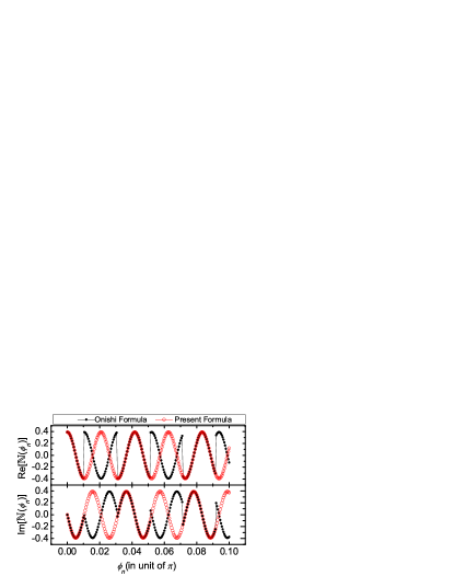
Figure 1: (Color online) Overlaps of the ground state neutron slater determinant for ²²⁶Th as functions of $\phi_{n}$ with Euler angles $\alpha=\gamma=0^{\circ},\beta=10^{\circ}$, calculated with present formula [Eq.(40)] and the Onishi formula [Eq.(52) with ‘+’ sign]. Re$[\mathbb{N}(\phi_{n})]$ and Im$[\mathbb{N}(\phi_{n})]$ are the real and imaginary parts of the overlap.

However, for the Onishi formula of Eq.(52), we do not need to change $v_{i}=0$ to $v_{i}=\varepsilon$. The overlaps for the neutron part, calculated with Eq.(40) and Eq.(52), are compared in Fig.1. The curves of Eq.(40) are continuous, but the sign uncertainty of Eq.(52) causes the discontinuity. However, if one copies the sign of Eq.(40) to Eq.(52), one can compare numerical difference between Eq.(40) and Eq.(52) using the following quantity, $R$,

$$R=\left|\frac{\mathbb{N}_{\mathrm{Onishi}}(\phi_{n})}{\mathbb{N}_{\mathrm{pf}}(\phi_{n})}-1\right|.$$ (53)

In all calculations, we found that $R<10^{-12}$ with double precision. This confirms that a small change of $v_{i}$ from zero to $\varepsilon$ almost does not affect numerical accuracy. However, it is crucial to keep Eq.(40) valid. Yet notice that $\mathbb{N}_{\mathrm{pf}}(\Xi)$ in Eq.(40) is obtained from a product of tiny and giant numbers. The same calculations have also been done with Eq.(31), and we also get $R<10^{-12}$. Thus we have presented an alternative way of using Eq.(31), where we set $v_{i}=\varepsilon$ for those empty orbits rather than omitting them[7].

Once the overlap is available, it is straightforward to perform the symmetry restoration. The deformed BCS vacuum of ²²⁶Th has been projected onto good particle number and spin. Therefore, one can test how precise the numerical calculations with Eq.(40) satisfy

$$\sum_{N,Z,I}\langle\psi|\hat{P}^{N}\hat{P}^{Z}\hat{P}^{I}_{00}|\psi\rangle=1,$$ (54)

where $\hat{P}^{N}$, $\hat{P}^{Z}$, and $\hat{P}^{I}_{MK}$ are neutron-number, proton-number, and spin projection operators, respectively. For the above vacuum state without pairing (i.e. the ground state slater determinant), the particle numbers of both neutrons and protons are good. Indeed, our particle number projection (using 16 mesh points in the integral) shows that $\langle\psi_{n}|\hat{P}^{N}|\psi_{n}\rangle=1$ ($N=96$), or 0 ($N\neq 96$) with numerical errors less than $10^{-13}$. Calculations for the protons also have the same accuracy. This again shows the reliability of Eq. (40). Angular momentum projection is also performed on the same state in addition to the particle number projection. The amplitude of $\langle\psi|\hat{P}^{N}\hat{P}^{Z}\hat{P}^{I}_{00}|\psi\rangle$ with ($N=96,Z=70$) is plotted as a function of spin $I$ in Fig.2. In the integral of the spin projection, 100 mesh points are taken, and the range of spin is $0\leq I\leq 70$, and we indeed reproduced Eq.(54) with numerical error around $10^{-12}$.

Figure 2: The amplitude of projection, $\langle\psi|\hat{P}^{N}\hat{P}^{Z}\hat{P}^{I}_{00}|\psi\rangle$, as a function of spin $I$ at $N=96$ and $Z=70$ using Eq.(40). $|\psi\rangle$ is the axially deformed BCS vacuum but without pairing.

We also have tested Eq.(40) in the projection of the triaxially deformed vacuum with normal pairing, which seems more convenient to use Eq.(40). With the present method, similar accuracy has also been achieved.

4 Summary

Following the strategy of Bertsch and Robledo [7], we have proposed a new formula of the overlap between HFB vacua by using the Pfaffian identity and assuming that the inverse of the $V$ matrix exists. This formula is especially convenient and efficient in the symmetry restoration, and has the same high accuracy as the Onishi formula as well as the correct sign. The reliability of the present formula has been tested by carrying out the calculations of the overlap and the quantum number projection for the heavy nucleus ²²⁶Th. In the testing calculations, one has to be faced with two numerical problems: (1) The extreme (huge or tiny) quantities are certainly encountered, and we have properly treated this situation to avoid data overflow (see the text). (2) For those empty orbits with $v_{i}=0$, which make Eq.(40) invalid, one can change $v_{i}$ to a small quantity $\varepsilon(>0)$ to avoid the singularity of $V$ matrix. It turns out that such treatments work very well. Testing calculations have confirmed that the present formula is even applicable to the pure slater determinant without losing the numerical accuracy. Thus it is promising that Eq.(40) may be applicable in evaluating the overlap between arbitrary HFB vacua.

Acknowledgements Z. G. thanks Prof. Y. Sun and Dr. F. Q. Chen for the stimulating and fruitful discussions. The authors acknowledge support from the National Natural Science Foundation of China under Contract Nos. 11175258, 11021504 and 11275068.

References

• [1] R. Balian and E. Brezin, Nuovo Cimento B 64 (1969) 37.
• [2] K. Hara, S. Iwasaki, Nucl. Phys. A 332 (1979) 61.
• [3] M. Oi, T. Mizusaki, Phys. Lett. B 707 (2012) 305.
• [4] T. Mizusaki, M. Oi, Phys. Lett. B 715 (2012) 219.
• [5] T. Mizusaki, M. Oi, Fang-Qi Chen, Yang Sun, Phys. Lett. B 725 (2013) 175.
• [6] B. Avez, M. Bender, Phys. Rev. C. 85 (2012) 034325.
• [7] G.F. Bertsch and L.M. Robledo, Phys. Rev. Lett. 108 (2012) 042505.
• [8] S. Perez-Martin and L.M. Robledo, Phys. Rev. C 76 (2007) 064314.
• [9] M. Anguiano, J.L. Egido, L.M. Robledo, Nucl. Phys. 696 (2001) 467.
• [10] N. Onishi and S. Yoshida, Nucl. Phys. 80 (1966) 367.
• [11] K. NeergΓ₯rd and E. WΓΌst, Nucl. Phys. A 402 (1983) 311.
• [12] Q. Haider and D. Gogny, J. Phys. G: Nucl. Part. Phys. 18 (1992) 993.
• [13] F. DΓΆnau, Phys. Rev. C 58 (1998) 872.
• [14] M. Bender and Paul-Henri Heenen, Phys. Rev. C 78 (2008) 024309.
• [15] K. Hara, A. Hayashi and P. Ring, Nucl. Phys. A 385 (1982) 14.
• [16] M. Oi and N. Tajima, Phys. Lett. B 606 (2005) 43.
• [17] L.M. Robledo, Phys. Rev. C 79 (2009) 021302(R).
• [18] L.M. Robledo, Phys. Rev. C 84 (2011) 014307.
• [19] P. Ring and P. Schuck, The Nuclear Many-Body Problem, Springer-Verlag, 1980.
• [20] K.W. Schmid, Prog. Part. Nucl. Phys. 52 (2004) 565.
• [21] K. Hara and Y. Sun, Int. J. Mod. Phys. E 4 (1995) 637.
• [22] T. Bengtsson and I. Ragnarsson, Nucl. Phys. A 436 (1985) 14.