A Convergence Theorem for the Graph Shift-type Algorithms

Abstract

Graph Shift (GS) algorithms are recently focused as a promising approach for discovering dense subgraphs in noisy data. However, there are no theoretical foundations for proving the convergence of the GS Algorithm. In this paper, we propose a generic theoretical framework consisting of three key GS components: simplex of generated sequence set, monotonic and continuous objective function and closed mapping. We prove that GS algorithms with such components can be transformed to fit the Zangwill’s convergence theorem, and the sequence set generated by the GS procedures always terminates at a local maximum, or at worst, contains a subsequence which converges to a local maximum of the similarity measure function. The framework is verified by expanding it to other GS-type algorithms and experimental results.

1 Introduction

The Graph Shift (GS) Algorithm[15] is a newly proposed algorithm in seeking the dense subgraph (also known as graph mode) and has received many attentions in machine learning and data mining area. As its tremendous advantages in removing the noise points in learning the dense subgraph, it is popularly used in image processing areas such as common pattern matching [14][23], computer vision area such as object tracking[21][3][13][20], cluster analysis[15], etc. Also, its low computation time and memory complexity make the realisty application feasible and attracted, especially in large-scale data size case. However, little theoretical work has been done to strengthen the solidness of the algorithm except for empirical demonstration, and to be honestly speaking, the correctness of the result always lays in doubt without theoretical guarantees.

The GS Algorithm originates from the the Dominant Sets and Pairwise Clustering(DSPC) Algorithm[16][17], which treated the dense subgraph discovery problem as a constrained optimization problem and gave a solid definition on the so-called "dominant set", i.e., dense subgraph. Further modifies the existing DSPC procedure, the GS Algorithm adds a neighborhood expansion procedure to reinforce the learning result. By iteratively employing the Replicator Dynamics and the new added "Neighborhood Expansion", the GS Algorithm claims to find the local maximum of the constraint objective function after finite number of iterations and further empirically demonstrates the claim.

However, to the best of our knowledge, none of the existing theoretical work has been done to certify the claim, nor does issues including the objective functions’ behavior during the procedures, the stopping criteria. All of the above issues are closely related to one thing: the GS Algorithms’ convergence property. That is to say, we need to ensure that the generated sequence set is convergent or at least contains a convergent subsequence set. It is certainly crucial to have a theoretical analysis about the GS Algorithm’s convergence before we can confidently utilize it.

Convergence theorem of algorithms has been a long-time discussion topic since decades ago in literature, including the ones with an iterative sequence set. Take the fuzzy $c$-means algorithm(FCM) for instance. The original strict proof is Provided by Bedzek [2][8], who employed the Zangwill’s theory [22][6] to establish the sequence’s convergence property. Hoppner[10] proved the convergence of the axis-parallel variant of the Gustafson-Kessel’s algorithm[7] by applying the Banach’s classical contraction principle[11], which is the general case of FCM. Groll[5] used the equivalence between the original and reduced FCM criteria, and conducted a new and more direct derivation of the convergence properties of FCM algorithms. Besides these, Selim[18] treated the k-means clustering problem as a nonconvex mathematical program and provided a rigorous proof of the finite convergence of the K-means-type algorithms.

It may be intuitive that the FCM’s convergence discussion could be applied to the GS Algorithm for both of them operating on an iterative set. However, it is not straightforward in implementation as the hardness of capturing GS Algorithm’s complex characters. To address this problem, we provide a theoretical analysis of the algorithm. We start with the understanding of principal characteristics of the GS Algorithm by breaking it down into three key components, including generated sequence set, objective function and mapping, and then propose a framework to map such components to the conditions required in the Zangwill’s theorem. We find that the mapped GS Algorithm can then perfectly match with the key requirements in the Zangwill’s theorem. The convergence theorem for the GS Algorithm is then brought about.

Furthermore, a definition of the so-called "GS-type algorithm" is then given to provide us with a general view of algorithms with similar properties. More importantly, we build up a systematic learning on them by analyzing the objective functions’ behaviors and observing their interesting resulting in the implemental results. We illustrate the proposed convergence theorem in terms of proving both the the GS Algorithm [15] and the DSPC Algorithm [17], and confirm with the experimental results.

After all, our contributions here are listed as follows:

1. We theoretically analyze the convergence behavior of the GS Algorithm.

2. We have proven both the GS Algorithm and the DSPC Algorithm terminates a local maximum value, or at least contains a subsequence which converges to a local maximum.

3. A convergence proof framework is builded to make a better generalization of our work.

The paper is organized as follows. Section 2 introduces the principle of the GS Algorithm and also a details description of it. In Section 3, we first introduce the Zangwill’s convergence theorem, and then extracts three key components in the GS Algorithm, mapping them to the Zangwill’s properties. Section 4 discusses the convergence of the GS Algorithm and also analyzes some features of the algorithm. We extend the convergence proof to other GS-type algorithms and build up a framework in Section 5. Experiments are conducted in Section 6 to verify the convergence theorem and behavior. Conclusions and future work can be found in Section 7.

2 Preliminaries

2.1 Rationale of the GS Algorithm

The basic principle of the Graph Shift Algorithm is set forth in the work of [15]. In the perspective of graph mining, the GS Algorithm aims at searching each vertex’s dense "nearer" subgraph with strong internal closeness. Two procedures of Replicator Dynamics and Neighborhood Expansion are recursively employed on each vertex sequentially to reach the goal. The former largely shrinks the identified subgraph, and the later expands the existing subgraph, both shift towards a local graph mode.

In [15][17], a probabilistic coordinate on Graph $G$ is defined as a mapping: $X:V\to\Delta^{n}$, where $\Delta^{n}=\{\boldsymbol{x}\in R^{n}:\boldsymbol{x}_{i}\geq 0,i\in\{1,\cdots,n\}~{}\textrm{and}~{}|\boldsymbol{x}|_{1}=1\}$, the support of $\boldsymbol{x}\in\Delta^{n}$ is the indices of all non-zero components, denoted as $\delta(\boldsymbol{x})=\{i|\boldsymbol{x}_{i}\neq 0\}$, corresponding to a subgraph $G_{\delta(\boldsymbol{x})}$, and $\boldsymbol{x}_{i}$ denotes node $i$’s attendance in the subgraph $G_{\delta(\boldsymbol{x})}$ to some extent.

The algorithm operates on an affinity matrix $A=(a_{ij})^{n\times n}$, in which $a_{ij}$ measures the similarity between node $i$ and node $j$. Then subgraph $G_{\delta(\boldsymbol{x})}$’s internal similarity is expressed as:

$$g(\boldsymbol{x}):=a(\boldsymbol{x},\boldsymbol{x})=\sum_{i,j=1}^{n}a_{ij}\boldsymbol{x}_{i}\boldsymbol{x}_{j}=\boldsymbol{x}^{T}A\boldsymbol{x}.$$ (1)

Accordingly, a local maximum solver of $g(\boldsymbol{x})$ can be taken to represent the desired dense subgraph. The identification of such local maximum regions is equivalent to solving the following quadratic optimization problem:

$$\left\{\begin{array}[]{lc}\textrm{maximize}&g(\boldsymbol{x})=\boldsymbol{x}^{T}A\boldsymbol{x}\\ \textrm{subject to}&\boldsymbol{x}\in\Delta^{n}\end{array}\right.$$ (2)

2.2 Mapping definition

We begin the discussion with a formal definition on the Graph Shift Algorithm and its corresponding mapping. These clear predefined related concepts would facilitate much on the problem statement and understanding.

In general, the GS Algorithm defines a mapping $T_{m}:\Delta^{n}\to\Delta^{n}$ to get the iterative sequence set as:

$$\boldsymbol{x}^{(k)}=T_{m}(\boldsymbol{x}^{(k-1)})=\cdots=(T_{m})^{(k)}(\boldsymbol{x}^{(0)});k=1,2,\cdots.$$ (3)

Where $\boldsymbol{x}^{(0)}$ is an initial starting point, and superscripts in parentheses correspond to the iteration number. Therefore, the problem of this paper is whether or not the iterative sequence set $\{\boldsymbol{x}^{(k)}\}_{k=1}^{\infty}$ generated by $T_{m}$ converges to a local maximum solver of problem (Equation (2)).

Specifying the mapping $T_{m}$ more clearly will be both necessary and of great help in analyzing this question. Accordingly, $T_{m}$, the combination of Replicator Dynamics procedure $(B^{m_{k}})$ and Neighborhood Expansion procedure$(C)$, is broken down as:

$$T_{m}:=B^{m_{k}}\circ C.$$ (4)

In Equation (4), $B^{m_{k}}$ represents the $k$-th ($k\leq m$) Replicator Dynamics procedure; $m_{k}$ corresponds to transformation $B$’s number in the $k$-th Replicator Dynamics procedure when a subgraph’s mode is reached in this procedure (this result is actually a special case of Theorem 3); $B$ is the transformation expressed as:

$$\begin{split}B:&\Delta^{n}\to\Delta^{n},\boldsymbol{x}(l_{k})\to\boldsymbol{x}(l_{k}+1)\\ =&(\frac{\omega_{1}(l_{k})\boldsymbol{x}_{1}(l_{k})}{\sum_{i=1}^{n}\omega_{i}(l_{k})\boldsymbol{x}_{i}(l_{k})},\cdots,\frac{\omega_{n}(l_{k})\boldsymbol{x}_{n}(l_{k})}{\sum_{i=1}^{n}\omega_{i}(l_{k})\boldsymbol{x}_{i}(l_{k})}).\end{split}$$ (5)

In Equation (5), $\omega_{i}(l_{k})=(A\boldsymbol{x}(l_{k}))_{i}=\sum_{j=1}^{n}a_{ij}\boldsymbol{x}_{j}(l_{k})$, $i\in\{1,\cdots,n\}$, $l_{k}\in\{1,\cdots,m_{k}-1\}$.

$C$ is the Neighborhood Expansion procedure, denoted as:

$$\boldsymbol{x}^{(k+1)}=\boldsymbol{x}^{(k)}+\Delta\boldsymbol{x}=\boldsymbol{x}^{(k)}+t^{*}\boldsymbol{b}.$$ (6)

Details of $t^{*}$ and $\boldsymbol{b}$ are explained in Appendix A.

2.3 Detail Procedure and Stopping Criteria

The GS Algorithm[15] is an iterative process through the loop in seeking the dense subgraph starting from each vertex in the graph, with the pseudo-code shown below illustrating the whole process.

0:  $A^{n\times n}$, Affinity matrix of the whole data set with the diagonal value 0;$\{\boldsymbol{x}=\{\boldsymbol{x}_{i}\}_{i=1^{n}}\},$ initial starting points, usually taken as $\{\boldsymbol{e}=\{\boldsymbol{e}_{i}\}_{i=1^{n}}\}$

1:  for i=1,…n do

2:     do Replicator Dynamics(Equation (5)) of $\boldsymbol{x}_{i}$

3:     if (result $\boldsymbol{x}$ is the mode of graph) then

4:        go to step 11

5:     end if

6:     do Neighborhood Expansion(Equation (6)) of $\boldsymbol{x}_{i}$

7:     if (result $\boldsymbol{x}$ is the mode of graph) then

8:        go to step 11

9:     end if

10:  end for

11:  return  the belonging clusters $\boldsymbol{c}=\{\boldsymbol{c}_{i}\}_{i=1}^{n}$ corresponding to the starting points $\boldsymbol{x}=\{\boldsymbol{x}_{i}\}_{i=1}^{n}$.

The stopping criteria of the algorithm , or the solution set of the problem (Equation (2)) is set to satisfy the Karush-Kuhn-Tucker (KKT) condition [12]:

$$\Gamma:=\{\boldsymbol{x}\in\Delta~{}|~{}\boldsymbol{x}~{}\textrm{satisfies}~{}(A\boldsymbol{x})_{i}\left\{\begin{array}[]{cc}=\lambda,&i\in\sigma(\boldsymbol{x});\\ \leq\lambda,&i\notin\sigma(\boldsymbol{x}).\end{array}\right.\}.$$ (7)

Here $(A\boldsymbol{x})_{i}$ is the $i$-th component of $A\boldsymbol{x}$; $\lambda$ is one Lagrange multiplier. $\sigma(\boldsymbol{x})=\{i\in\{1,\cdots,n\}|\boldsymbol{x}_{i}\neq 0\}$ corresponds to the subgraph as defined above.

As stated above, the GS Algorithm is implemented on each vertex’s evolving process by recursively using the Replicator Dynamics procedure and Neighborhood Expansion Procedure, until it reaches the desired solution, i.e., satisfying KKT condition (Equation (7)) to each of the starting vertices.

3 Mapping from the GS Algorithm to the Zangwill’s Theorem

The Zangwill’s convergence theorem [22][6] is fundamental in terms of proving the convergence of iterative sets for its general applicability. In this section, we build up the mapping from the GS principle to the Zangwill’s convergence theorem.

3.1 Zangwill’s Convergence Theorem

Definitions and lemmas are introduced before we present the Zangwill’s convergence theorem.

Definition 1

A point-to-set mapping $\Omega$ from set $X$ to power set $Y$ is defined as $\Omega:X\to P(Y)$, which associates a subset of $Y$ with each point in $X$, $P(Y)$ denotes the power set of $Y$.

Definition 2

Given a function $f$ and an element $c$ of the domain $I$, $f$ is said to be continuous at the point $c$ if the following holds: for every $\varepsilon>0$, there exists a $\eta>0$ such that for all $x\in I$, $|x-c|<\eta\Rightarrow|f(x)-f(c)|<\varepsilon$.

Definition 3

A point-to-set mapping $\Omega:X\to P(Y)$ is said to be closed at a point $\boldsymbol{x}^{*}$ in $X$ if $\{\boldsymbol{x}^{(m)}\}\subset X$ and $\boldsymbol{x}^{(m)}\to\boldsymbol{x}^{*},\boldsymbol{y}^{(m)}\in\Omega(\boldsymbol{x}^{(m)})$ and $\boldsymbol{y}^{(m)}\to\boldsymbol{y}^{*}$ imply that $\boldsymbol{y}^{*}\in\Omega(\boldsymbol{x}^{*})$.

The following Lemma 1 is induced by integrating a continuous function with a point-to-set mapping:

Lemma 1

Let $C:M\to V$ be a function and $B:V\to P(V)$ be a point-to-set mapping. Assume $C$ is continuous at $\omega^{*}$ and $B$ is closed at $C(\omega^{*})$, then the point-to-set mapping $A=B\circ C:M\to P(V)$ is closed at $\omega^{*}$.

The composition of continuous functions is still a continuous function, we have Lemma 2:

Lemma 2

Given two continuous functions: $f:I\to J(\subset\boldsymbol{r}),g:J\to\boldsymbol{R}$, the composition $g\circ f:I\to\boldsymbol{R},x\mapsto g(f(x))$ is continuous.

Accordingly, the Zangwill’s convergence theorem is described below.

Theorem 1

Given an algorithm on $X$, $\boldsymbol{x}^{(0)}\in X$, assume the sequence $\{\boldsymbol{x}^{(k)}\}_{k=1}^{\infty}$ is generated which satisfies

$$\boldsymbol{x}^{(k+1)}\in\boldsymbol{A}(\boldsymbol{x}^{(k)})$$ (8)

For a given solution set $\Gamma\subset X$ of an algorithm, if the following three properties holds:

The Zangwill’s convergence theorem provide a feasible direction to verify one algorithm’s convergence behavior, especially ones with iterative implementations. With its general flexibility, it has been applied widely to prove the convergence of algorithms with similar properties, including clustering and optimization research. Amongst all the iterative algorithms, here we are interested, in particular, in monotonic algorithms.

3.2 Mapping

Retrospective to the conditions in Zangwill’s theorem, we further break down the GS Algorithm and abstract the following characteristics from it (detailed verification will be given later):

1), Simplex of generated sequence set

The candidate solution sequence set $\{\boldsymbol{x}^{(k)}\}_{k=0}^{\infty}$ generated by the mapping $T_{m}$ lies in $\Delta^{n}=\{\boldsymbol{x}\in R^{n}:\boldsymbol{x}_{i}\geq 0$ and $|\boldsymbol{x}|_{1}=1\}$, i.e., the standard $n$-simplex of $R^{n}$ in any step $k$ ($k\leq m$);

2), Monotonic and continuous objective function

The objective function $g(\boldsymbol{x})=\boldsymbol{x}^{T}A\boldsymbol{x}$ is continuous and strictly increases during the mapping $T_{m}$ according to the Propositions 2-4.3 (see Section 4);

3), Closed mapping

The mapping $T_{m}=B^{m_{k}}\circ C$ is closed during each procedure in accordance to Propositions 4.4-4.5 (see Section 4) at all points of the generated sequence set.

These three properties are also the key components in one algorithm, that is to say, with these vital feature requirements clearly prescribed, the algorithm is fixed into a predefined framework, including the generated sequence set defining the scope of the variables, the objective function’s behavior describing the algorithm mapping’s efforts towards the setting goal and mapping itself with restricted property.

Table 1. depicts the one-to-one correspondence similarities between these two more clearly.

Table 1: Mapping between GS Algorithm and Zangwill’s Theorem

the GS Algorithm		the Zangwill’s theorem
${Simplex}$	$\thicksim$	${Compact}$
${Monotonic}$	$\thicksim$	${Decreasing}$
${Closed}$	$\thicksim$	${Closed}$

4 Convergence of the GS Algorithm

Several propositions are declared before analyzing deeply into the convergence behavior of the GS Algorithm, all focus on the three properties as we discussed in Section 2. Detailed proofs of these propositions are given in Appendix B-E.

The GS Algorithm’s stable solution set is compact according to Proposition 1.

Proposition 1

The sequence set $\{\boldsymbol{x}^{(k)}\}_{k=0}^{\infty}\subset S$ generated by the mapping $T_{m}=B^{m_{k}}\circ C$ is a compact set.

Propositions 2-4.3 discuss the monotonicity of $g(\boldsymbol{x})$ under the mapping $T_{m}=B^{m_{k}}\circ C$, as discussed about the monotonicity of the GS Algorithm’s main characteristics.

Proposition 2

The objective function $f(\boldsymbol{x})=\boldsymbol{x}^{T}\boldsymbol{A}\boldsymbol{x}$ strictly increases along any nonconstant trajectory of Equation (5) when $\boldsymbol{x}\in X/\Gamma$.

Proposition 3

The objective function $f(\boldsymbol{x})=\boldsymbol{x}^{T}\boldsymbol{A}\boldsymbol{x}$ strictly increases along the neighborhood expansion operation of Equation (6).

Proof 4.2.

It can be derived from the definition of $\Delta\boldsymbol{x}$ in Appendix B.

Proposition 4.3.

$g(x)=\boldsymbol{x}^{T}A\boldsymbol{x}$ is a function both continuous and strictly increasing during the mapping $T_{m}=B^{m_{k}}\circ C$ when $\boldsymbol{x}\in X/\Gamma$, but just increasing if $\boldsymbol{x}\in\Gamma$.

Propositions 4.4-4.5 validate the closed mapping property of the GS Algorithm.

Proposition 4.4.

The mapping $C$ is closed on all points of $X\backslash\Gamma$.

Proposition 4.5.

The mapping $T_{m}=B^{m_{k}}\circ C$ is closed on $X/\Gamma$.

Proof 4.6.

According to the definition of $B$ (Equation (5)), it is continuous on $X/\Gamma$. C is closed on $X/\Gamma$ as per Proposition 4.4. According to Lemma 1, $T_{m}$ is closed on $X/\Gamma$.

With the above preparations, we have the following Theorem 2.

Theorem 4.7.

Let $A=(a_{ij})^{(n\times n)}$ be a similarity matrix with diagonal values 0, $T_{m}$, $\Gamma$ be defined as Equation $(\ref{t_eq7})$, Equation $(\ref{t_eq3})$, and $\boldsymbol{x}^{(0)}$ be an arbitrary initial starting point, then either the iteration sequence $\{\boldsymbol{x}^{(r)}\}$ ($r=1,2,\ldots$) terminates at a point $\boldsymbol{x}^{*}$ in the solution set $\Gamma$ or there is a subsequence converging to a point in $\Gamma$.

Proof 4.8.

Taking $\hat{g}(\boldsymbol{x})=-g(\boldsymbol{x})=-\boldsymbol{x}^{T}A\boldsymbol{x}$ as the continuous function $Z$ and $T_{m}$ as the algorithm mapping $A$ in Theorem 1. Proposition 1 shows that the sequence set $\{\boldsymbol{x}^{(k)}\}_{k=1}^{\infty}$ generated by $T_{m}$ is a compact set. $\hat{g}(\boldsymbol{x})$ is continuous and strict decreasing as the continuity and strict increasing characteristic of $g(\boldsymbol{x})$ in the trajectory of $T_{m}$ are proven by Proposition 4.3. Proposition 4.5 asserts $T_{m}$ is closed on $x/\Gamma$ ($\Gamma$ is the solution set defined in Equation (7)). According to the Zangwill’s convergence theory, Theorem 2 holds as all three properties are satisfied.

This result gives us the theoretical guarantees to the various applications of the GS Algorithm and ensure to reach at least a local maximum of the objective function after finite number of algorithm’s mapping implementations.

5 Convergence for Other GS-type Algorithms

We expand the proposed GS convergence theorem’s proof to other GS-type algorithms. Take the Dominant Sets and Pairwise Clustering (DSPC) Algorithm [17] as an example, for it is the origin method of the GS Algorithm. The DSPC Algorithm shares the same goal as the GS Algorithm in terms of finding dense subgraphs, i.e., dominant sets $\sigma(\boldsymbol{x})$. Their implementations are mostly similar, however differentiates in whether selecting the neighborhood expansion or not, the GS Algorithm does but the DSPC Algorithm does not.

The detail implementation of the DSPC Algorithm could refer to [17], due to the simiplicy, we ignore it here and focus on its convergence behavior. The DSPC Algorithm consists of three key components, holding similar properties to the GS Algorithm, however, differing in minor places.

1), Simplex of generated sequence set

The sequence set $\{\boldsymbol{x}^{(k)}\}_{k=0}^{\infty}$ generated by mapping $B$ always lies in $\Delta^{n}$;

2), Monotonic and continuous objective function

The objective function $g(\boldsymbol{x})=\boldsymbol{x}^{T}A\boldsymbol{x}$ is continuous and strictly increasing during the mapping $B$;

3), Continuous mapping

The mapping $B$ is continuous.

Table 2 further displays the relationship between the DSPC Algorithm, the GS Algorithm and the Zangwill’s theorem.

Table 2: GS-type algorithms and Zangwill’s theorem’s mapping

DSPC Algorithm		GS Algorithm		Zangwill’s theorem
$Simplex$	$\thicksim$	$Simplex$	$\thicksim$	$Compact$
${Monotonic}$	$\thicksim$	${Monotonic}$	$\thicksim$	$Decreasing$
${Continuous}$	$\thicksim$	${Closed}$	$\thicksim$	$Closed$

A convergence proof has been provided for the continuous version of the DSPC Algorithm in [19]. Here some related propositions are first introduced. Then we discuss the convergence property of its discrete-time version by involving the Zangwill’s convergence theorem.

Proposition 5.9.

The sequence set $\{\boldsymbol{x}^{(k)}\}_{k=0}^{\infty}\subset S$ generated by the mapping $B^{m_{k}}$ is a compact set.

For its proof, refer to Appendix B.

Proposition 5.10.

If a mapping $f:S\to T$ is continuous on $S$, then $f$ is closed on $S$.

Theorem 5.11.

Let $A=(a_{ij})^{(n\times n)}$ be a similarity matrix with diagonal values 0, $B$ be defined as Equation $(\ref{t_eq8})$, and $\boldsymbol{x}^{(0)}$ be an arbitrary initial starting point, then either the iteration sequence $\{\boldsymbol{x}^{(r+1)}=B(\boldsymbol{x}^{(r)})\},(r=1,2,\ldots)$ terminates at a point $\boldsymbol{x}^{*}$ in the solution set $\Gamma$ or there is a subsequence converging to a point in $\Gamma$.

Proof 5.12.

Taking $\hat{g}(\boldsymbol{x})=-g(\boldsymbol{x})=-\boldsymbol{x}^{T}A\boldsymbol{x}$ as the continuous function $Z$ and $B$ as the algorithm mapping $A$ in Theorem 1. Proposition 5.9 shows that the sequence set $\{\boldsymbol{x}^{(k)}\}_{k=1}^{\infty}$ generated by $B$ is a compact set. $\hat{g}(\boldsymbol{x})$ is continuous and strict decreasing according to the continuity and strict increase of $g(\boldsymbol{x})$ in the trajectory of $T_{m}$ are proven in Proposition 2. Proposition 5.10 asserts $B$ is closed on $x/\Gamma$, while $\Gamma$ is the solution set defined in in Equation (7). According to the Zangwill’s convergence theory, Theorem 3 holds.

There are many similarities shared between these two algorithms’ proving process, along with their similar properties. Thus, we can propose a Zangwill’s theorem-based convergence framework for the "similar algorithms". Firstly, the so-called "GS-type algorithm" is defined referring to what we called "similar algorithms".

Definition 5.13.

An algorithm is a GS-type algorithm if and only if it satisfies the conditions on three key components: simplex of generated sequence set, monotonic and continuous objective function and closed mapping.

We provide a flowchart (Fig. 1) to illustrate our prooving process in details. It presents a guideline proving the convergence of GS-type algorithms step by step. (1) Break down the GS-type algorithm into three parts: generated set, objective function and mapping. (2) Check if these three parts all satisfy the corresponding requirements. Any part unsatisfied is regarded as unsuitable for applying this framework, otherwise it is convergent.

Figure 1: Proving framework for GS-type algorithm convergence

Among the two processes in Fig. 1, properties verification is usually the difficult part, especially the objective function’s monotonic behavior. We will further discuss its behavior in the Section 6.

6 Experimental Verification

The GS Algorithm and the DSPC Algorithm are all implemented in MATLAB2011b. Our experiments are conducted on an Acer Aspire 4720Z laptop having an Intel Pentium DualCoreT2330(1.6GHz, 533MHz FSB, 1MB L2 cache), with 2GB DDR2 RAM, using LINUX operating system.

6.1 Experimental Settings

Since GS-type algorithms manipulate data based on a similarity matrix, we construct a similarity matrix instead of real data sets with its element values uniformly sampling within the interval $[0,1]$, and the matrix dimensionality scaling from $100$ to $3000$. Also, we consider cases in which the matrices are fully dense matrices (FDM), partially dense matrices (PDM), and block tridiagonal matrices (BTM).

Initial starting point $\boldsymbol{x}$ can be randomly chosen or be the single vertice $\{I_{i},i=1,\cdots,n.\}$. In our experiments, we use the single vertice with the same as [14]. We test the GS Algorithm [15] as well as the DSPC Algorithm [17]. Each algorithm runs for three times to obtain an averaged performance. We verify the proposed the GS Algorithm convergence theory through experiments and focus on testing convergence performance. The number of transformations ($m_{k}$) in Replicator Dynamics, the whole iteration number ($m$), running time ($T$), and average iteration running time ($t=T/m$) are presented to evaluate the convergence performance.

Table 3: the GS Algorithm and the DSPC Algorithm’s testing results

the GS Algorithm							the DSPC Algorithm
Case	Scale	$m_{k}$	$m$	$T(s)$	$t(s)$	S.R.(%)1	Case	Scale	$m_{k}$	$T(s)$	S.R.(%)1
FDM	100	1228.5	2.52	0.12	0.05	100.0	FDM	100	953.2	0.14	100.0
	500	1297.3	2.96	0.40	0.14	100.0		500	1298.5	0.37	100.0
	1000	1101.7	3.75	1.01	0.27	100.0		1000	1604.2	1.10	100.0
	1500	1401.2	3.24	3.87	1.19	100.0		1500	1469.6	4.25	100.0
	2000	1575.4	3.49	20.00	5.73	100.0		2000	1448.1	18.61	100.0
	3000	1511.4	3.56	50.15	14.09	100.0		3000	1785.3	56.20	100.0
PDM	100	236.3	2.22	0.02	0.01	26.1	PDM	100	203.3	0.02	26.7
	500	285.9	2.24	0.08	0.04	26.2		500	299.6	0.07	26.3
	1000	275.4	2.38	0.20	0.09	26.4		1000	326.7	0.15	26.4
	1500	275.9	2.40	0.94	0.39	26.4		1500	338.2	0.55	26.3
	2000	348.1	2.41	3.32	1.38	26.3		2000	288.8	2.11	26.4
	3000	332.9	2.50	7.75	3.10	26.3		3000	389.3	6.85	26.3
BTM	100	794.9	2.16	0.06	0.03	22.0	BTM	100	717.6	0.05	22.0
	500	1185.3	2.65	0.31	0.12	22.0		500	1177.7	0.28	22.0
	1000	1221.6	2.67	0.68	0.25	22.0		1000	1130.8	0.74	22.0
	1500	1198.6	2.97	2.96	1.00	22.0		1500	1226.5	2.63	22.0
	2000	1289.9	3.02	13.57	4.50	22.1		2000	1417.8	13.24	22.0
	3000	1406.2	3.13	38.55	12.34	22.0		3000	1517.4	38.16	22.0

• S.R. refers to the sparse rate, the proportion of the number of non-zero elements to the number of whole elements.

6.2 Objective function behavior

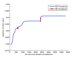
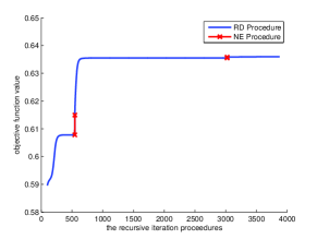
Figure 2: Vertex 71(left), 231(middle) and 265(right)’s objective functions’ behaviors(For better view, please see color pdf.)

Fig. 2 depicts the behaviors of three representative vertices’ corresponding objective function in the GS Algorithm under the PDM case and 500 scale, along with the candidate solution evolving. The $X$-axis represents the evolving process times , and the $Y$-axis stands for the objective function’s value. To be fairly compare the performance, we take $B$ and $C$’s time as equal. Thus, the rate of evolving time is $m_{k}:1$ between Replicator Dynamics and Neighborhood Expansion in the $k$-th iteration, according to Equation (4).

From these three vertices’ evolving behaviors, we can see all the three vertices reach a local maximum value. The objective function’s value kept increasing with the evolving process, which is in accordance with the Proposition 4.3. This is perfectly matched with the theorem we have proposed.

When the curve first starting from the Replicator Dynamics, it always produces a steep increasing trends in the first few steps and then turn to a gentle curve in the last. What is more, when encounters the Neighborhood Expansion procedure, it always produce a huge jump comparing to the flat curve in the Replicator Dynamics. This is because the Neighborhood Expansion procedure is one that pulling the candidate solution from one local dense subgraph towards the dense graph and the dense value will change much with the subgraph changes.

Also, we can notice that most of the evolving time is the Replicator Dynamics, denoting that most of the calculations were done in Replicator Dynamics, i.e., searching the dense subgraph.

6.3 Convergence performance

The convergence performance of the GS Algorithm and the DSPC Algorithm depends on many factors: scale of the affinity matrix, matrix structure, element value, etc. We test different scenarios by changing the scale of matrix and the sparseness of matrix. The scenarios and results are given in Table 3.

The experimental results presented in the GS Algorithm and the DSPC Algorithm are a little different for their different mapping definitions, with the former being $T_{m}=B^{m_{k}}\circ C$ and the later being $B$.

The results show that both the GS Algorithm and the DSPC Algorithm converge under the cases with FDM, PDM and BTM. In each case, transformation $B$’s number $m_{k}$ and iteration $T_{m}$’s number $m$ increase slowly when matrix’s scaling grows, sometimes even with a small drop, e.g., in FDM case of the GS Algorithm, $m_{k}$’s values in the third row and $m$’s value in the fourth row are both smaller than the previous ones although matrices’ scale increases. What is more, when the matrice’s scale is 3000, which is 30 times of the first one’s scale in each case, its $m_{k}$ and $m$’s values are less than 2 times larger. This indicates that if the dense rate of the matrix is fixed, the computational cost is always under control even though the matrices’ scale increases.

Also, the GS Algorithm’s transformation number, iteration number and running time all decrease when the matrix becomes sparser, the same with the DSPC Algorithm’s transformation number and running time. This indicates that if we incorporate prior information and setting the unrelated nodes’ similarity value as 0, then we can save much computational cost in the application. However, both of the two Algorithms performs worse on the block tridiagonal matrices case compared to the partially dense matrices case, even with a smaller sparse rate. This is due to the fact that block tridiagonal matrices’ calculation is quite similar to the one of smaller scale with full dense matrices. As shown above, it is heavily computational loaded.

7 Conclusions and Future work

Graph Shift (GS) Algorithm shows great advantage on efficiently dealing with noisy data, however no theoretical outcome has been reported about its algorithm behavior and what is more, its convergence proof. In this paper, we have proposed a generic theoretical framework to prove the convergence of GS-type algorithms. A GS-type Algorithm consists of three key components: simplex of generated sequence set, monotonic and continuous objective function and closed mapping. They are mapped to the Zangwill’s convergence theorem’s three key conditions. Consequently, the convergence of the GS Algorithm is proved by applying the Zangwill convergence theorem.

We have shown that the framework can be applied to GS-type algorithms, as well as the Dominant set and pairwise clustering (DSPC) Algorithm. Experimental results on both the GS Algorithm and the DSPC Algorithm certified that they both converge under different scenarios in terms of the scale of the affinity matrix, the transformation number, and the iteration number.

However, this paper limits the generated sequence set under the simplex case, more work will be done to expand it to other compact set. What is more, Banach’s contraction theory and optimization methods on nonconvex mathematical program are being considered in our problem so as to suit in a more general case.

Appendix A Definition of $\Delta\boldsymbol{x}$

According to [15], $\Delta\boldsymbol{x}=t^{*}\boldsymbol{b}$, $t^{*}$ and $\boldsymbol{b}$ are defined as:

$$\boldsymbol{b}=\left\{\begin{array}[]{cc}-\boldsymbol{x}_{i}s&i\in\sigma(\boldsymbol{x});\\ v_{i},&i\notin\sigma(\boldsymbol{x}).\end{array}\right.$$ (9)

$$t^{*}=\left\{\begin{array}[]{cc}\frac{1}{s},&\textrm{if}~{}\lambda s^{2}+2s\zeta-\omega\leq 0\\ \textrm{min}(\frac{1}{s},\frac{\zeta}{\lambda s^{2}+2s\zeta-\omega}),&\textrm{if}~{}\lambda s^{2}+2s\zeta-\omega>0\end{array}\right.$$ (10)

where

$$v_{i}=\left\{\begin{array}[]{cc}0,&i\in\sigma(\boldsymbol{x})\\ \textrm{max}(a(\boldsymbol{x},I_{i})-g(\boldsymbol{x}),0),&i\notin\sigma(\boldsymbol{x})\end{array}\right.$$ (11)

$$s=\sum_{i\notin\sigma(\boldsymbol{x})}v_{i},\zeta=\sum_{i\notin\sigma(\boldsymbol{x})}v_{i}^{2},\omega=\sum_{i,j}v_{i}a_{ij}v_{j}.$$ (12)

$g(\boldsymbol{x}+\Delta\boldsymbol{x})-g(\boldsymbol{x})=-(\lambda s^{2}+2s\zeta-\omega)t^{2}+2\zeta t$. When $\lambda s^{2}+2s\zeta-\omega\leq 0$, $g(\boldsymbol{x}+\Delta\boldsymbol{x})-g(\boldsymbol{x})\geq 0$; When $\lambda s^{2}+2s\zeta-\omega<0$, $t^{*}$ always lies in the interval $[0,\frac{2\zeta}{\lambda s^{2}+2s\zeta-\omega}]$, which are the two solutions of $g(\boldsymbol{x}+\Delta\boldsymbol{x})-g(\boldsymbol{x})=0$, this leads to $g(\boldsymbol{x}+\Delta\boldsymbol{x})-g(\boldsymbol{x})>0$.

Appendix B Proof of Proposition 1

Proof B.14.

To prove that the sequence set $\{\boldsymbol{x}_{(k)}\}_{k=0}^{\infty}\subset S$ is compact is equivalent to prove that the set is bounded and closed. Since $(\boldsymbol{x}_{1},\boldsymbol{x}_{2},\cdots,\boldsymbol{x}_{n})$ are all located in $[0,1]$, the $\boldsymbol{x}$ value space is bounded. Also, from Equation (5), $\boldsymbol{e}_{i}=(0,...,1,...,0)$, which means the $i$-th component of $\boldsymbol{x}$ is 1 and the others are 0, we can denote $\boldsymbol{x}(t)$ as:

$$\boldsymbol{x}(t)=\sum_{i=1}^{n}\boldsymbol{e}_{i}\cdot\frac{\boldsymbol{x}(t-1)_{i}(A\boldsymbol{x}_{i}(t-1))}{\boldsymbol{x}(t-1)^{T}A\boldsymbol{x}(t-1)}$$ (13)

Since $\sum_{i=1}^{n}\frac{\boldsymbol{x}(t-1)_{i}(A\boldsymbol{x}_{i}(t-1))}{\boldsymbol{x}(t-1)^{T}A\boldsymbol{x}(t-1)}=1$ and $0\leq\frac{\boldsymbol{x}(t-1)_{i}(A\boldsymbol{x}_{i}(t-1))}{\boldsymbol{x}(t-1)^{T}A\boldsymbol{x}(t-1)}\leq 1,i=1,\ldots,n.$. Adding $\Delta\boldsymbol{x}$ (defined in Appendix A) still holds the expression $\boldsymbol{x}(t)=\sum_{i=1}^{n}\boldsymbol{e}_{i}\cdot y_{i},\sum_{i=1}^{n}y_{i}=1$, thus $\boldsymbol{x}(t)$ is in the convex hull of $S$, so it is closed. Therefore, the sequence set $\{\boldsymbol{x}_{(k)}\}_{k=0}^{\infty}\subset S$ is both bounded and closed.

Appendix C Proof of Proposition 2

Proof C.15.

This proposition is known in mathematical biology as the fundamental theory of natural selection [9] and, in its original form, we can trace it back to [4].

We can also prove that Proposition 2 is a special case of Baum-Eagon inequality ([1]). We denote $x_{i}$ as $x_{i}=\prod_{j=1}^{n}x_{j}^{\mu_{ij}}$, here $\mu_{ij}=\left\{\begin{array}[]{cc}1,&i=j;\\ 0,&i\neq j.\end{array}\right.$. Thus we wish to prove that when $\boldsymbol{x}(t)\notin\Gamma$:

$$\begin{split}g(x)=&x^{T}Ax=\sum_{i=1}^{n}\omega_{i}x_{i}=\sum_{i=1}^{n}\omega_{i}\prod_{j=1}^{n}x_{j}^{\mu_{ij}}\\ &<\sum_{i=1}^{n}\omega_{i}\prod_{j=1}^{n}J(x_{j})^{\mu_{ij}}.\end{split}$$ (14)

From Hölder inequation and $x_{i}^{2}=x_{i}\cdot\prod_{j=1}^{n}x_{j}^{\mu_{ij}}$, we can get the result as:

$$\begin{split}g(x)&=\sum_{i=1}^{n}\{\omega_{i}\cdot\prod_{j=1}^{n}J(x_{j})^{\mu_{ij}}\}^{\frac{1}{2}}\times\{\omega_{i}^{\frac{1}{2}}x_{i}\prod_{j=1}^{n}(\frac{1}{J(x)})^{\frac{\mu_{ij}}{2}}\}\\ &\leq\{\sum_{i=1}^{n}\omega_{i}\prod_{j=1}^{n}J(x_{j})^{\mu_{ij}}\}^{\frac{1}{2}}\times\{\sum_{i=1}^{n}\omega_{i}x_{i}\prod_{j=1}^{n}(\frac{x_{j}}{J(x_{j})})^{\mu_{ij}}\}^{\frac{1}{2}}\end{split}$$ (15)

Equality holds if and only if $\forall p,q\in\{1,\cdots,n\}$,

$$\begin{split}&\frac{\{\omega_{p}\cdot\prod_{j=1}^{n}J(x_{j})^{\mu_{{p}j}}\}^{\frac{1}{2}}}{\omega_{p}^{\frac{1}{2}}x_{p}\prod_{j=1}^{n}(\frac{1}{J(x)})^{\frac{\mu_{{p}j}}{2}}}=\frac{\{\omega_{q}\cdot\prod_{j=1}^{n}J(x_{j})^{\mu_{{q}j}}\}^{\frac{1}{2}}}{\omega_{q}^{\frac{1}{2}}x_{q}\prod_{j=1}^{n}(\frac{1}{J(x)})^{\frac{\mu_{{q}j}}{2}}}\\ \iff&\frac{J(x_{p})}{x_{p}}=\frac{J(x_{q})}{x_{q}}\iff\omega_{p}=\omega_{q}\end{split}$$ (16)

Using the inequality of geometric and arithmetic means to the double products of the second brace, we can conclude:

$$\begin{split}&\sum_{i=1}^{n}\omega_{i}x_{i}\prod_{j=1}^{n}(\frac{x_{j}}{J(x_{j})})^{{\mu_{ij}}}\leq\sum_{i=1}^{n}\omega_{i}x_{i}\sum_{j=1}^{n}{\mu_{ij}}\cdot\frac{x_{j}}{J(x_{j})}\\ &=\sum_{i=1}^{n}\omega_{i}x_{i}\sum_{j=1}^{n}\mu_{ij}x_{j}\cdot\frac{\sum_{k=1}^{n}\omega_{k}x_{k}}{\omega_{j}x_{j}}\\ &=\sum_{k=1}^{n}\omega_{k}x_{k}\cdot\sum_{j=1}^{n}x_{j}\cdot\frac{\sum_{i=1}^{n}\omega_{i}x_{i}\cdot\mu_{ij}}{\omega_{j}x_{j}}\\ &=\sum_{k=1}^{n}\omega_{k}x_{k}\cdot\sum_{j=1}^{n}x_{j}=\sum_{k=1}^{n}\omega_{k}x_{k}.\end{split}$$ (17)

Equality holds if and only if $\forall p,q\in\{1,\cdots,n\}$,

$$\frac{x_{p}}{J(x_{p})}=\frac{x_{p}}{J(x_{p})}~{}\iff~{}\omega_{p}=\omega_{q}.$$ (18)

Here the last equation succeed because $\omega_{i}x_{i}\cdot\mu_{ij}=\omega_{j}x_{j}$ if and only if $j=i$, otherwise it is $0$, and $\sum_{j=1}^{n}x_{j}=1.$

we put the result into the second braces, and get

$$\begin{split}&\sum_{i=1}^{n}\omega_{i}x_{i}\leq\{\sum_{i=1}^{n}\omega_{i}\prod_{j=1}^{n}J(x_{j})^{\mu_{ij}}\}^{\frac{1}{3}}\times\{\sum_{i=1}^{n}\omega_{i}x_{i}\}^{\frac{2}{3}}\\ \iff&\{\sum_{i=1}^{n}\omega_{i}x_{i}\}^{\frac{1}{3}}\leq\{\sum_{i=1}^{n}\omega_{i}\prod_{j=1}^{n}J(x_{j})^{\mu_{ij}}\}^{\frac{1}{3}}\\ \iff&\sum_{i=1}^{n}\omega_{i}x_{i}\leq\sum_{i=1}^{n}\omega_{i}\prod_{j=1}^{n}J(x_{j})^{\mu_{ij}}\end{split}$$ (19)

Equality holds if and only if $\omega_{i}=\omega_{j},\forall i,j\in\{1,\cdots,n\}$. It is the situation contained by the solution set $\Gamma$.
Thus, the function $g(x)=\boldsymbol{x}^{t}A\boldsymbol{x}$ is strictly increasing along any nonconstant trajectory of (5) when $\boldsymbol{x}\in X/\Gamma$.

Appendix D Proof of Proposition 4

Proof D.16.

The continuity of $g(\boldsymbol{x})=\boldsymbol{x}^{T}A\boldsymbol{x}$ is obvious. We here discuss the increasing monotonicity. From Equation (4), we have

$$g(\boldsymbol{x})\leq g(C(\boldsymbol{x}))<g(B\circ C(\boldsymbol{x}))=g(T_{m}(\boldsymbol{x}))$$ (20)

Appendix E Proof of Proposition 5

Proof E.17.

If $\boldsymbol{x}^{0}\in X$, then $\boldsymbol{x}^{n}\to\boldsymbol{x}^{0}$ and $\boldsymbol{y}^{n}\to\boldsymbol{y}^{0}$ when $n\to\infty$. Consequently $\boldsymbol{y}^{n}\in C(\boldsymbol{x}^{n})$, indicating that

$$\boldsymbol{y}^{n}=\boldsymbol{x}^{n}+\Delta\boldsymbol{x}^{n}$$ (21)

and we need to prove that

$$\boldsymbol{y}^{0}=C(\boldsymbol{x}^{0})=\boldsymbol{x}^{0}+\Delta\boldsymbol{x}^{0}.$$ (22)

This lies in two situations:

1. $\boldsymbol{x}^{0}$ is in $\Gamma$, thus $\Delta\boldsymbol{x}^{0}\ =0$.

2. $\boldsymbol{x}^{0}$ is in $X\backslash\Gamma$.

For situation (2), as $\boldsymbol{x}^{n}\to\boldsymbol{x}^{0}$ and $\boldsymbol{y}^{n}\to\boldsymbol{y}^{0}$, we can find a large $N$ such that $\forall\varepsilon>0,\exists n>N,~{}\textrm{so that}~{}|\boldsymbol{x}^{n}-\boldsymbol{x}^{0}|<\varepsilon,|\boldsymbol{y}^{n}-\boldsymbol{y}^{0}|<\varepsilon$. Consequently, we have

$$\begin{split}&|\boldsymbol{y}^{0}-C(\boldsymbol{x}^{0})|\leq|\boldsymbol{y}^{0}-\boldsymbol{y}^{n}|+|\boldsymbol{y}^{n}-C(\boldsymbol{x}^{n})|+|C(\boldsymbol{x}^{n})\\ &-C(\boldsymbol{x}^{0})|\leq\varepsilon+|\boldsymbol{x}^{n}-\boldsymbol{x}^{0}|+|\Delta\boldsymbol{x}^{0}-\Delta\boldsymbol{x}^{n}|\\ &\leq 2\varepsilon+|\Delta\boldsymbol{x}^{0}-\Delta\boldsymbol{x}^{n}|\\ \end{split}$$ (23)

According to Lemma 2 and the definitions of $\boldsymbol{b}$ and $t$, it is a continuous mapping on $\boldsymbol{x}$, this results in that $\forall\varepsilon>0,\exists\delta$ such that $|\Delta\boldsymbol{x}^{0}-\Delta\boldsymbol{x}^{n}|\leq\varepsilon$. So, $\forall\varepsilon>0$, if $N_{1}$ is big enough, $n>N_{1},|\boldsymbol{x}^{n}-\boldsymbol{x}^{0}|<$min$(\varepsilon/3,\delta)$, $|\boldsymbol{y}^{n}-\boldsymbol{y}^{0}|<\varepsilon/3$, then

$$|\boldsymbol{y}^{0}-C(\boldsymbol{x}^{0})|\leq\varepsilon$$ (24)

Hence $\boldsymbol{y}^{0}=C(\boldsymbol{x}^{0})$, and $C$ is closed on $X\backslash\Gamma$.

References

- [1] L. Baum and J. Eagon. An inequality with applications to statistical estimation for probabilistic functions of markov processes and to a model for ecology. Bull. Amer. Math. Soc, 73(3):360–363, 1967.
- [2] J. Bezdek. A convergence theorem for the fuzzy isodata clustering algorithms. Pattern Analysis and Machine Intelligence, IEEE Transactions on, (1):1–8, 1980.
- [3] T. Chen, S. Jiang, L. Chu, and Q. Huang. Detection and location of near-duplicate video sub-clips by finding dense subgraphs. In Proceedings of the 19th ACM international conference on Multimedia, pages 1173–1176. ACM, 2011.
- [4] R. Fisher. The genetical theory of natural selection. 1930.
- [5] L. Groll and J. Jakel. A new convergence proof of fuzzy -means. Fuzzy Systems, IEEE Transactions on, 13(5):717–720, 2005.
- [6] A. Gunawardana and W. Byrne. Convergence theorems for generalized alternating minimization procedures. The Journal of Machine Learning Research, 6:2049–2073, 2005.
- [7] D. Gustafson and W. Kessel. Fuzzy clustering with a fuzzy covariance matrix. In Decision and Control including the 17th Symposium on Adaptive Processes, 1978 IEEE Conference on, volume 17, pages 761–766. IEEE, 1978.
- [8] R. Hathaway, J. Davenport, and J. Bezdek. Relational duals of the -means clustering algorithms. Pattern recognition, 22(2):205–212, 1989.
- [9] J. Hofbauer and K. Sigmund. Evolutionary games and population dynamics. Cambridge University Press, 1998.
- [10] F. Hoppner and F. Klawonn. A contribution to convergence theory of fuzzy -means and derivatives. Fuzzy Systems, IEEE Transactions on, 11(5):682–694, 2003.
- [11] V. Istratescu. Fixed point theory an introduction, volume 7. Kluwer Academic Print on Demand, 2002.
- [12] H. W. Kuhn and A. W. Tucker. Nonlinear programming. In Proceedings, Second Berkeley Symposium in Mathematical Statistics and Probability, J. Neyman, editor. University of California Pres, Berkeley, Calif, pages 481–92, 1951.
- [13] X. Li, A. Dick, H. Wang, C. Shen, and A. van den Hengel. Graph mode-based contextual kernels for robust svm tracking. In Computer Vision (ICCV), 2011 IEEE International Conference on, pages 1156–1163. IEEE, 2011.
- [14] H. Liu and S. Yan. Common visual pattern discovery via spatially coherent correspondences. In Computer Vision and Pattern Recognition (CVPR), 2010 IEEE Conference on, pages 1609–1616. IEEE, 2010.
- [15] H. Liu and S. Yan. Robust graph mode seeking by graph shift. In International Conference on Machine Learning, 2010.
- [16] M. Pavan and M. Pelillo. A new graph-theoretic approach to clustering and segmentation. In Computer Vision and Pattern Recognition, 2003. Proceedings. 2003 IEEE Computer Society Conference on, volume 1, pages I–145. IEEE, 2003.
- [17] M. Pavan and M. Pelillo. Dominant sets and pairwise clustering. Pattern Analysis and Machine Intelligence, IEEE Transactions on, 29(1):167–172, 2007.
- [18] S. Selim and M. Ismail. K-means-type algorithms: a generalized convergence theorem and characterization of local optimality. Pattern Analysis and Machine Intelligence, IEEE Transactions on, (1):81–87, 1984.
- [19] J. Weibull. Evolutionary game theory. The MIT press, 1997.
- [20] X. Yang, H. Liu, and L. Jan Latecki. Contour-based object detection as dominant set computation. Pattern Recognition, 2011.
- [21] J. Yuan, G. Zhao, Y. Fu, Z. Li, A. Katsaggelos, and Y. Wu. Discovering thematic objects in image collections and videos. Image Processing, IEEE Transactions on, (99):1–1, 2011.
- [22] W. Zangwill. Nonlinear programming: a unified approach. Prentice-Hall international series in management. Prentice-Hall, 1969.
- [23] J. Zhao, J. Ma, J. Tian, J. Ma, and D. Zhang. A robust method for vector field learning with application to mismatch removing. In Computer Vision and Pattern Recognition (CVPR), 2011 IEEE Conference on, pages 2977–2984. IEEE, 2011.