Constructing New Realisable Lists from Old in the NIEP

Abstract

Given a list of complex numbers $\sigma:=(\lambda_{1},\lambda_{2},\ldots,\lambda_{m})$, we say that $\sigma$ is realisable if $\sigma$ is the spectrum of some (entrywise) nonnegative matrix. The Nonnegative Inverse Eigenvalue Problem (or NIEP) is the problem of categorising all realisable lists.

Given a realisable list $(\rho,\lambda_{2},\lambda_{3},\ldots,\lambda_{m})$, where $\rho$ is the Perron eigenvalue and $\lambda_{2}$ is real, we find families of lists

$$(\mu_{1},\mu_{2},\ldots,\mu_{n}),$$

for which

$$(\mu_{1},\mu_{2},\ldots,\mu_{n},\lambda_{3},\lambda_{4},\ldots,\lambda_{m})$$

is realisable. In addition, given a realisable list

$$(\rho,\alpha+i\beta,\alpha-i\beta,\lambda_{4},\lambda_{5},\ldots,\lambda_{m}),$$

where $\rho$ is the Perron eigenvalue and $\alpha$ and $\beta$ are real, we find families of lists $(\mu_{1},\mu_{2},\mu_{3},\mu_{4}),$ for which

$$(\mu_{1},\mu_{2},\mu_{3},\mu_{4},\lambda_{4},\lambda_{5},\ldots,\lambda_{m})$$

is realisable.

AMS classification: 15A18, 15A29

Keywords: Nonnegative matrices, Nonnegative Inverse Eigenvalue Problem, Companion matrix

1 Introduction

We denote the spectrum of a matrix $A$ by $\sigma(A)$. We say that $A$ is nonnegative if it is entrywise nonnegative and in this case we write $A\geq 0$. In general, if $A,B\in\mathbb{R}^{n\times n}$ or $y,z\in\mathbb{R}^{n}$, we will use notation such as $A\geq B$ or $y\geq z$ if the inequalities hold entrywise. For a list of complex numbers $\sigma:=(\lambda_{1},\lambda_{2},\ldots,\lambda_{n})$, we define $s_{m}(\sigma):=\sum_{i=1}^{n}\lambda_{i}^{m}$. $I_{n}$ denotes the $n\times n$ identity matrix.

We call $\sigma$ realisable if there exists a nonnegative matrix $A$ with spectrum $\sigma$ and in this case, we say that $A$ realises $\sigma$. The Nonnegative Inverse Eigenvalue Problem (or NIEP) is the problem of categorising all realisable lists.

We begin by stating some well-known necessary conditions for a list to be realisable. Let $\sigma:=(\lambda_{1},\lambda_{2},\ldots,\lambda_{n})$ be the spectrum of a nonnegative matrix $A$. Then

1. $\sigma$ is closed under complex conjugation, i.e. $\overline{\sigma}:=\left(\overline{\lambda_{1}},\overline{\lambda_{2}},\ldots,\overline{\lambda_{n}}\right)=\sigma;$

2. $\max_{i}|\lambda_{i}|\in\sigma;$

3. $s_{m}(\sigma)\geq 0$ for every positive integer $m$;

4. $s_{k}(\sigma)^{m}\leq n^{m-1}s_{km}(\sigma)$ for all positive integers $k$ and $m$.

Condition (i) follows from the fact that the characteristic polynomial of $A$ has real coefficients. Condition (ii) says that the spectral radius of $A$, $\rho$ say, is an eigenvalue of $A$. This result forms part of the well-known Perron-Frobenius theory of nonnegative matrices. The eigenvalue $\rho$ is known as the Perron eigenvalue of $A$ and the corresponding eigenvector is known as the Perron eigenvector. We will always write the Perron eigenvalue as the first entry in a realisable list. Condition (iii) follows from the fact that $s_{m}(\sigma)$ is the trace of $A^{m}$. The inequalities in (iv) are called the JLL conditions. They were proved by Loewy and London [10] and independently by Johnson [5].

We denote by $e$ the vector of appropriate size with every entry equal to 1, i.e. $e:=[\begin{array}[]{cccc}1&1&\cdots&1\end{array}]^{T}$. The following useful result—due to Johnson [5]—allows us to assume without loss of generality that the Perron eigenvector of a realising matrix is $e$. A proof can also be found in [4].

Lemma 1.1.

[5] Let $A$ be a nonnegative matrix with Perron eigenvalue $\rho$. Then there exists a nonnegative matrix $B$, cospectral with $A$, satisfying $Be=\rho e$.

In the case where all eigenvalues but the Perron have nonpositive real parts, the NIEP has been completely solved by Laffey and Šmigoc [8]:

Theorem 1.2.

[8] Let $\rho\geq 0$ and let $\lambda_{2},\lambda_{3},\ldots,\lambda_{n}$ be complex numbers such that $\mathrm{Re}\,\lambda_{i}\leq 0$ for all $i=2,3,\ldots,n$. Then the list $\sigma=(\rho,\lambda_{2},\lambda_{3},\ldots,\lambda_{n})$ is the spectrum of a nonnegative matrix if and only if the following conditions are satisfied:

1. $\sigma$ is closed under complex conjugation;

2. $s_{1}(\sigma)\geq 0$;

3. $s_{1}(\sigma)^{2}\leq ns_{2}(\sigma)$.

Furthermore, when the above conditions hold, $\sigma$ may be realised by a matrix of the form $G+\gamma I_{n}$, where $G$ is a nonnegative companion matrix with trace zero and $\gamma$ is a nonnegative scalar.

Remark.

The condition that $\mathrm{Re}\,\lambda_{i}\leq 0$ for all $i=2,3,\ldots,n$ in Theorem 1.2 can be relaxed to $\mathrm{Re}\,\lambda_{i}\leq s_{1}(\sigma)/n$. To see this, note that the quantity

$$ns_{2}(\sigma)-s_{1}(\sigma)^{2}$$

is unchanged by subtracting a scalar from $\sigma$, i.e.

$$ns_{2}(\rho-\delta,\lambda_{2}-\delta,\ldots,\lambda_{n}-\delta)-s_{1}(\rho-\delta,\lambda_{2}-\delta,\ldots,\lambda_{n}-\delta)^{2}\\ =ns_{2}(\rho,\lambda_{2},\ldots,\lambda_{n})-s_{1}(\rho,\lambda_{2},\ldots,\lambda_{n})^{2}$$

for all $\delta\in\mathbb{C}$ and hence if $(\rho,\lambda_{2},\ldots,\lambda_{n})$ satisfies (i)–(iii), then so does $(\rho-s_{1}(\sigma)/n,\lambda_{2}-s_{1}(\sigma)/n,\ldots,\lambda_{n}-s_{1}(\sigma)/n)$.

The results in this paper fall into the category of constructing new realisable lists from known realisable lists. We give some earlier results of this type below. Guo [4] gave the following theorem regarding the perturbation of a realisable list:

Theorem 1.3.

[4] If $(\rho,\lambda_{2},\lambda_{3},\ldots,\lambda_{n})$ is realisable, where $\rho$ is the Perron eigenvalue and $\lambda_{2}$ is real, then

$$(\rho+\delta,\lambda_{2}\pm\delta,\lambda_{3},\lambda_{4},\ldots,\lambda_{n})$$

is realisable for all $\delta\geq 0$.

To generalise Theorem 1.3 to the perturbation of non-real eigenvalues, we have the following theorem. Result (1) is due to Laffey [6] and an alternative proof can be found in [3]. Result (2) is due to Guo and Guo [3].

Theorem 1.4.

If $(\rho,\alpha+i\beta,\alpha-i\beta,\lambda_{4},\lambda_{5},\ldots,\lambda_{n})$ is realisable, where $\rho$ is the Perron eigenvalue and $\alpha$ and $\beta$ are real, then for all $\delta\geq 0$, the lists

$$(\rho+2\delta,\alpha-\delta+i\beta,\alpha-\delta-i\beta,\lambda_{4},\lambda_{5},\ldots,\lambda_{n})$$ (1)

and

$$(\rho+4\delta,\alpha+\delta+i\beta,\alpha+\delta-i\beta,\lambda_{4},\lambda_{5},\ldots,\lambda_{n})$$ (2)

are realisable.

Šmigoc [11] gives a different kind of perturbation, in which the Perron eigenvalue of a realisable list may be replaced by a new list:

Theorem 1.5.

[11] Let $(\rho,\lambda_{2},\lambda_{3},\ldots,\lambda_{m})$ be realisable, where $\rho$ is the Perron eigenvalue and let $(\mu_{1},\mu_{2},\ldots,\mu_{n})$ be the spectrum of a nonnegative matrix with a diagonal element greater than or equal to $\rho$. Then

$$(\mu_{1},\mu_{2},\ldots,\mu_{n},\lambda_{2},\lambda_{3},\ldots,\lambda_{m})$$

is realisable.

In [12], Šmigoc gives a construction to replace both the Perron eigenvalue and another real eigenvalue:

Theorem 1.6.

[12] Let $(\rho,\lambda_{2},\lambda_{3},\ldots,\lambda_{m})$ be realisable, where $\rho$ is the Perron eigenvalue and $\lambda_{2}$ is real. Let $a$ and $t_{1}$ be any nonnegative numbers and let $t_{2}$ be any real number such that $|t_{2}|\leq t_{1}$. Then

$$(\mu_{1},\mu_{2},\mu_{3},\lambda_{3},\lambda_{4},\ldots,\lambda_{m})$$

is realisable, where $\mu_{1},\mu_{2},\mu_{3}$ are the roots of the polynomial

$$w(x)=(x-\rho)(x-\lambda_{2})(x-a)-(t_{1}+t_{2})x+t_{1}\lambda_{2}+t_{2}\rho.$$

In Section 2, we expand on the work done in [12] by presenting some new lists which may replace the eigenvalues $\rho$ and $\lambda_{2}$. In Section 3, we give a construction which allows us to replace the Perron eigenvalue and a complex conjugate pair of eigenvalues, i.e. given a realisable list

$$(\rho,\alpha+i\beta,\alpha-i\beta,\lambda_{4},\lambda_{5},\ldots,\lambda_{m}),$$

where $\rho$ is the Perron eigenvalue and $\alpha$ and $\beta$ are real, we find some conditions on the list $(\mu_{1},\mu_{2},\mu_{3},\mu_{4})$ which imply that

$$(\mu_{1},\mu_{2},\mu_{3},\mu_{4},\lambda_{4},\lambda_{5},\ldots,\lambda_{m})$$

is realisable.

To this end, we begin by giving a Lemma from [12], which is the foundation of this work:

Lemma 1.7.

[12] Let the following assumptions hold:

1. $Y$ is an invertible matrix with a partition $Y=\left[\begin{array}[]{cc}Y_{1}&Y_{2}\end{array}\right],$ where $Y_{1}$ is an $m\times p$ matrix and $Y_{2}$ is an $m\times m_{1}$ matrix with $p+m_{1}=m$;

2. $B$ is an $m\times m$ matrix such that

   $$Y^{-1}BY=\left[\begin{array}[]{cc}C&E\\ 0&F\end{array}\right]$$

   for a $p\times p$ matrix $C$ and an $m_{1}\times m_{1}$ matrix $F$;

3. $M$ is an $n\times n$ matrix with a principal submatrix $C$, partitioned in the following way:

   $$M=\left[\begin{array}[]{cc}A&K\\ L&C\end{array}\right],$$

   where $A$ is an $n_{1}\times n_{1}$ matrix and $p+n_{1}=n$;

4. $K=HY_{1}$ for an $n_{1}\times m$ matrix $H$.

Then for matrices

$$N=\left[\begin{array}[]{cc}A&H\\ Y_{1}L&B\end{array}\right]\;\;\text{and}\;\;Z=\left[\begin{array}[]{cc}I_{n_{1}}&0\\ 0&Y\end{array}\right],$$

we have

$$Z^{-1}NZ=\left[\begin{array}[]{ccc}A&K&HY_{2}\\ L&C&E\\ 0&0&F\end{array}\right].$$

In particular, Lemma 1.7 produces a matrix $N$ with spectrum $\sigma(N)=(\sigma(M),\sigma(F))$. In order to apply this construction to the NIEP, it is necessary to determine when the matrix $N$ produced in this way is nonnegative. In [12], Šmigoc gives the following answer to this question:

For an $m\times p$ matrix $Y_{1}$, we define the sets:

$$\mathcal{L}(Y_{1}):=\{l\in\mathbb{R}^{p}:Y_{1}l\geq 0\}$$

and

$$\mathcal{K}(Y_{1}):=\{k\in\mathbb{R}^{p}:k^{T}=h^{T}Y_{1}\text{ for some nonnegative }h\in\mathbb{R}^{m}\}.$$

For a $p\times p$ matrix $C$ and an $m\times p$ matrix $Y_{1}$, we define $\mathcal{M}_{n}(Y_{1},C)$ to be the set of all $n\times n$ matrices

$$M=\left[\begin{array}[]{cc}A&K\\ L&C\end{array}\right],$$

such that $A$ is an $n_{1}\times n_{1}$ nonnegative matrix, $n=n_{1}+p$, every column of $L$ lies in $\mathcal{L}(Y_{1})$ and the transpose of every row of $K$ lies in $\mathcal{K}(Y_{1})$.

Theorem 1.8.

[12] Let the assumptions (i)–(iv) in Lemma 1.7 hold. Assume also that $B$ is nonnegative, that the Perron eigenvalue of $B$ lies in $\sigma(C)$ and that $M\in\mathcal{M}_{n}(Y_{1},C)$. Then the matrix $N$ of the lemma is nonnegative, i.e. the list $(\sigma(M),\sigma(F))$ is realisable by a nonnegative matrix with principal submatrices $A$ and $B$.

Theorem 1.8 provides a method of producing new realisable lists from old. With $p=1$, it allows us to replace the Perron eigenvalue of a known realisable list, for example as in Theorem 1.5. The $p=1$ case has been dealt with in detail in [11]. With $p=2$, it allows us to replace the Perron eigenvalue and another real eigenvalue, for example as in Theorem 1.6. The $p=2$ case is dealt with in [12] and we give further results in Section 2. With $p=3$, Theorem 1.8 allows us to replace the Perron eigenvalue and a complex conjugate pair of eigenvalues (see Section 3).

2 A $p=2$ construction

In this section, given a realisable list $(\rho,\lambda_{2},\lambda_{3},\ldots,\lambda_{m})$, where $\rho$ is the Perron eigenvalue and $\lambda_{2}$ is real, we present some lists $(\mu_{1},\mu_{2},\ldots,\mu_{n})$ such that $(\mu_{1},\mu_{2},\ldots,\mu_{n},\lambda_{3},\lambda_{4},\ldots,\lambda_{m})$ is realisable. This corresponds to letting $p=2$ in Lemma 1.7.

In [12], Šmigoc characterises $\mathcal{L}(Y_{1})$ and $\mathcal{K}(Y_{1})$ for the $p=2$ case. Using Lemma 1.1, we may assume without loss of generality that the eigenvector corresponding to $\rho$ is $e$. Let $z$ be a real eigenvector corresponding to $\lambda_{2}$ and let $z_{\mathrm{max}}$ and $z_{\mathrm{min}}$ denote the maximal and minimal entries of $z$, respectively. In [12], Section 4, Šmigoc shows that we may assume $z_{\mathrm{max}}>0$ and $z_{\mathrm{min}}\leq 0$. She then gives the following characterisations of $\mathcal{L}(Y_{1})$ and $\mathcal{K}(Y_{1})$:

Proposition 2.1.

[12] If $z_{\mathrm{max}}>0$ and $z_{\mathrm{min}}<0$, then

$$\mathcal{L}(Y_{1})=\left\{\left[\begin{array}[]{c}l_{1}\\ l_{2}\end{array}\right]:-\frac{l_{1}}{z_{\mathrm{max}}}\leq l_{2}\leq-\frac{l_{1}}{z_{\mathrm{min}}}\right\}.$$

If $z_{\mathrm{max}}>0$ and $z_{\mathrm{min}}=0$, then

$$\mathcal{L}(Y_{1})=\left\{\left[\begin{array}[]{c}l_{1}\\ l_{2}\end{array}\right]:-\frac{l_{1}}{z_{\mathrm{max}}}\leq l_{2}\text{ and }l_{1}\geq 0\right\}.$$

Proposition 2.2.

[12]

$$\mathcal{K}(Y_{1})=\left\{\left[\begin{array}[]{c}k_{1}\\ k_{2}\end{array}\right]:z_{\mathrm{min}}k_{1}\leq k_{2}\leq z_{\mathrm{max}}k_{1}\right\}.$$

We now give our $p=2$ construction.

Lemma 2.3.

Let the following assumptions hold:

1. the list $\sigma_{0}:=(\rho,\lambda_{2},\lambda_{3},\ldots,\lambda_{m})$ is realisable, where $\rho$ is the Perron eigenvalue, $\lambda_{2}$ is real and $\rho\neq\lambda_{2}$;

2. $C^{\prime}$ is a $2\times 2$ matrix of the form

   $$C^{\prime}:=\left[\begin{array}[]{cc}\gamma&1\\ b_{2}&b_{1}+\gamma\end{array}\right],$$

   where $b_{1}$ is real, $\gamma=(\rho+\lambda_{2}-b_{1})/2\geq 0$ and $b_{2}=\left((\rho-\lambda_{2})^{2}-b_{1}^{2}\right)/4$;

3. $K^{\prime}:=[\begin{array}[]{cc}f&g\end{array}]$, where $f,g\in\mathbb{R}^{n-2}$, $g\geq 0$ and $f\geq(\gamma-\lambda_{2})g$;

4. $L^{\prime}:=\left[\begin{array}[]{c}c^{T}\\ d^{T}\end{array}\right]$, where $c,d\in\mathbb{R}^{n-2}$, $c\geq 0$ and $d\geq(\rho-\gamma)c$;

5. $A$ is an $(n-2)\times(n-2)$ nonnegative matrix;

6. $M^{\prime}$ is the $n\times n$ matrix defined by

   $$M^{\prime}:=\left[\begin{array}[]{cc}A&K^{\prime}\\ L^{\prime}&C^{\prime}\end{array}\right].$$

Then the list $(\sigma(M^{\prime}),\lambda_{3},\lambda_{4},\ldots,\lambda_{m})$ is realisable.

Proof.

Let $B$ be a nonnegative matrix with spectrum $\sigma_{0}$. As in the construction of Lemma 1.7, let $Y$ be an invertible matrix such that

$$Y^{-1}BY=\left[\begin{array}[]{cc}C&*\\ 0&*\end{array}\right],$$

where

$$C:=\left[\begin{array}[]{cc}\rho&0\\ 0&\lambda_{2}\end{array}\right].$$

By Lemma 1.1, we may assume without loss of generality that the Perron eigenvector of $B$ is $e$. Let $z$ be a real eigenvector of $B$ corresponding to $\lambda_{2}$, appropriately scaled so that $z_{\mathrm{max}}=1$ and $z_{\mathrm{min}}\leq 0$ (see the discussion preceding Proposition 2.1) and let us write $Y=[\begin{array}[]{cc}Y_{1}&Y_{2}\end{array}]$, where $Y_{1}=[\begin{array}[]{cc}e&z\end{array}]$.

Note that the definitions of $\gamma$ and $b_{2}$ assure $\sigma(C^{\prime})=(\rho,\lambda_{2}).$ Therefore, since $\rho$ and $\lambda_{2}$ are distinct, we may diagonalise $C^{\prime}$. Indeed, $X^{-1}C^{\prime}X=C$, where

$$X:=\left[\begin{array}[]{cc}1&1\\ \rho-\gamma&\lambda_{2}-\gamma\end{array}\right]\>\text{ and }\>X^{-1}=\frac{1}{\rho-\lambda_{2}}\left[\begin{array}[]{cc}-\lambda_{2}+\gamma&1\\ \rho-\gamma&-1\end{array}\right].$$

Now define

$$K:=K^{\prime}X=\left[\begin{array}[]{cc}f+(\rho-\gamma)g&f+(\lambda_{2}-\gamma)g\end{array}\right],$$

$$L:=X^{-1}L^{\prime}=\frac{1}{\rho-\lambda_{2}}\left[\begin{array}[]{c}(-\lambda_{2}+\gamma)c^{T}+d^{T}\\ (\rho-\gamma)c^{T}-d^{T}\end{array}\right]$$

and

$$M:=\left[\begin{array}[]{cc}A&K\\ L&C\end{array}\right].$$

We will show that $M\in\mathcal{M}_{n}(Y_{1},C)$ and that $M$ and $M^{\prime}$ are similar (and hence cospectral). The result will then follow by Theorem 1.8.

To see that $M\in\mathcal{M}_{n}(Y_{1},C)$, we first note that since $g\geq 0$ and $f\geq(\gamma-\lambda_{2})g\geq(\gamma-\rho)g$, we have

$$z_{\mathrm{min}}\left(f+(\rho-\gamma)g\right)\leq 0\leq f+(\lambda_{2}-\gamma)g\leq f+(\rho-\gamma)g$$

and hence, by Proposition 2.2, the transpose of every row of $K$ lies in $\mathcal{K}(Y_{1})$. Similarly, since $c\geq 0$ and $d\geq(\rho-\gamma)c\geq(\lambda_{2}-\gamma)c$, we have that

$$-\left((-\lambda_{2}+\gamma)c+d\right)\leq(\rho-\gamma)c-d\leq 0\leq-\frac{1}{z_{\mathrm{min}}}\left((-\lambda_{2}+\gamma)c+d\right),$$

where the right-most inequality holds provided $z_{\mathrm{min}}\neq 0$. Then, by Proposition 2.1, every column of $L$ lies in $\mathcal{L}(Y_{1})$.

Therefore, we have shown that $M\in\mathcal{M}_{n}(Y_{1},C)$. Finally, it is easy to see that $M$ and $M^{\prime}$ are similar:

$$M=\left[\begin{array}[]{cc}I&0\\ 0&X\end{array}\right]^{-1}M^{\prime}\left[\begin{array}[]{cc}I&0\\ 0&X\end{array}\right].\qed$$

In the proof of Lemma 2.3, we have shown that $M^{\prime}$ is similar to a matrix in $\mathcal{M}_{n}(Y_{1},C)$. In the applications of this lemma, we will choose $A$, $K^{\prime}$ and $L^{\prime}$ in such a way that $M^{\prime}$ has a structure which makes its characteristic polynomial easy to compute. Several such structured matrices—such as companion matrices, doubly companion matrices and block companion matrices—have been studied in the context of the NIEP, for example by Friedland, Laffey, Šmigoc and Cronin [2], [9], [1] and indeed, the form of the matrix $C^{\prime}$ in Lemma 2.3 has been chosen with such matrices in mind.

For example, letting

$$A=\left[\begin{array}[]{cccc}\gamma&1&&\\ &\gamma&\ddots&\\ &&\ddots&1\\ &&&\gamma\end{array}\right],$$ (3)

$d\geq 0$, $f=[\begin{array}[]{ccccc}0&0&\cdots&0&1\end{array}]^{T}$ and $c=g=0$, the matrix $M^{\prime}$ becomes a companion matrix plus a scalar and as such, the characteristic polynomial of $M^{\prime}$ is easy to write down. The case where $M^{\prime}$ is a companion matrix plus a scalar is developed formally in Theorem 2.6.

Alternatively, keeping $c$, $d$, $f$ and $g$ as above, but setting

$$A=\left[\begin{array}[]{ccccccc}\gamma&1&&&&&\\ &\ddots&\ddots&&&&\\ &&\gamma&1&&&\\ &*&\cdots&*&1&&\\ &&&&\gamma&\ddots&\\ &&&&&\ddots&1\\ &&&&&&\gamma\\ \end{array}\right],$$

the matrix $M^{\prime}$ becomes a 2-block companion matrix plus a scalar.

Taking $f$, $g$ and $d$ as above, $c=[\begin{array}[]{ccccc}*&0&0&\cdots&0\end{array}]^{T}$ and

$$A=\left[\begin{array}[]{cccc}*&1&&\\ &\gamma&\ddots&\\ \vdots&&\ddots&1\\ &&&\gamma\end{array}\right],$$

then $M^{\prime}$ becomes a doubly companion matrix plus a scalar.

Example 2.4.

Let $\sigma$ be any list such that $(8,2,\sigma)$ is realisable. In Lemma 2.3, let us take $\rho=8$, $\lambda_{2}=2$, $b_{1}=10$ and $n=4$. It is easily verified that the matrices

$$K^{\prime}:=\left[\begin{array}[]{cc}0&0\\ 1&0\end{array}\right],\>\>L^{\prime}:=\left[\begin{array}[]{cc}42&0\\ 336&28\end{array}\right]\>\text{ and }\>A:=\left[\begin{array}[]{cc}0&1\\ 3&0\end{array}\right]$$

satisfy the hypotheses of the lemma and the matrix $M^{\prime}$ of the lemma then becomes

$$M^{\prime}=\left[\begin{array}[]{cccc}0&1&0&0\\ 3&0&1&0\\ 42&0&0&1\\ 336&28&-16&10\end{array}\right].$$

$M^{\prime}$ is a doubly companion matrix with characteristic polynomial

$$w(x) = x^{4}-10x^{3}+13x^{2}-40x+36$$

$$= (x-9)(x-1)(x^{2}+4)$$

and hence the list $(9,1,2i,-2i,\sigma)$ is realisable.

Example 2.5.

Let $\sigma$ be any list such that $(8,-2,\sigma)$ is realisable. In Lemma 2.3, take $\rho=8$, $\lambda_{2}=-2$, $b_{1}=6$ and $n=7$. Then the matrix

$$M^{\prime}=\left[\begin{array}[]{cc}A&K^{\prime}\\ L^{\prime}&C^{\prime}\end{array}\right]=\left[\vbox{\hbox{\kern-1.15198pt\raise 0.0pt\hbox{\kern 77.50008pt}\kern 0.0pt\vbox{}\kern-1.15198pt}}\right]$$

satisfies the hypotheses of the lemma. $M^{\prime}$ is an example of a 2-block companion matrix. Its characteristic polynomial is

$$w(x)=\frac{1}{29}\left(29x^{2}-203x-266\right)\left(x^{4}+64\right)(x+1)$$

and hence the list

$$(8.128\ldots,-1.128\ldots,2+2i,2-2i,-2+2i,-2-2i,-1,\sigma)$$

is realisable.

Theorem 2.6.

Let the list $\sigma_{0}:=(\rho,\lambda_{2},\lambda_{3},\ldots,\lambda_{m})$ be realisable, where $\rho$ is the Perron eigenvalue, $\lambda_{2}$ is real and $\rho\neq\lambda_{2}$. Let $b_{1}$ be any real number such that

$$\gamma:=\frac{\rho+\lambda_{2}-b_{1}}{2}\geq 0,$$ (4)

let

$$b_{2}:=\frac{(\rho-\lambda_{2})^{2}-b_{1}^{2}}{4}$$ (5)

and let $b_{3},b_{4},\ldots,b_{n}$ be any nonnegative numbers. Then the list

$$(\mu_{1},\mu_{2},\ldots,\mu_{n},\lambda_{3},\lambda_{4},\ldots,\lambda_{m})$$

is realisable, where $\mu_{1},\ldots,\mu_{n}$ are the roots of the polynomial

$$w(x):=(x-\gamma)^{n}-b_{1}(x-\gamma)^{n-1}-b_{2}(x-\gamma)^{n-2}-\cdots-b_{n-1}(x-\gamma)-b_{n}.$$

Proof.

In Lemma 2.3, let $A$ be as in (3) and let $d=[\begin{array}[]{cccc}b_{n}&b_{n-1}&\cdots&b_{3}\end{array}]^{T}$, $f=[\begin{array}[]{ccccc}0&0&\cdots&0&1\end{array}]^{T}$ and $c=g=0$. Then, note that $M^{\prime}-\gamma I_{n}$ becomes a companion matrix (where $M^{\prime}$ is defined in the statement of the lemma) and as such it has characteristic polynomial $w(x+\gamma)$. Hence $M^{\prime}$ has characteristic polynomial $w(x)$. ∎

Example 2.7.

Let $\sigma$ be any list such that $(4,2,\sigma)$ is realisable. Taking $\rho=4$ and $\lambda_{2}=2$ in Theorem 2.6, let us choose $n=4$, $b_{1}=6$, $b_{3}=10$ and $b_{4}=25$. Then, the polynomial $w(x)$ of the theorem becomes

$$w(x) = x^{4}-6x^{3}+8x^{2}-10x-25$$

$$= (x-5)(x^{2}-2x+5)(x+1)$$

and so the list $(5,1+2i,1-2i,-1,\sigma)$ is realisable.

At this point, we wish to use Theorem 1.2 in conjunction with Theorem 2.6 to produce a class of spectra which may replace the eigenvalues $\rho$ and $\lambda_{2}$; however, Theorem 1.2 deals with realisation by matrices of the form $G+\gamma I_{n}$, where $G$ has trace zero and so applying this directly would correspond to taking $b_{1}=0$ in Theorem 2.6. With this in mind, we will present a slight modification of Theorem 1.2, in which we examine realisation by a matrix of the form $G+\gamma I_{n}$, where $G$ may have nonzero trace. First, we will require a lemma from [8]:

Lemma 2.8.

[8] Let $b_{1}\geq 0$ and let $(\lambda_{2},\lambda_{3},\ldots,\lambda_{n})$ be a list of complex numbers, closed under complex conjugation and with nonpositive real parts. Set $\rho:=b_{1}-\lambda_{2}-\lambda_{3}-\cdots-\lambda_{n}$ and

$$f(x):=(x-\rho)\prod_{i=2}^{n}(x-\lambda_{i})=x^{n}-b_{1}x^{n-1}-b_{2}x^{n-2}-\cdots-b_{n}.$$

Then $b_{2}\geq 0$ implies $b_{i}\geq 0$ for all $i=3,4,\ldots,n$.

Theorem 2.9.

Let $\sigma:=(\rho,\lambda_{2},\lambda_{3},\ldots,\lambda_{n})$ be realisable, where $\rho$ is the Perron eigenvalue and $\mathrm{Re}\,\lambda_{i}\leq 0$ for all $i=2,3,\ldots,n$. Then for any nonnegative number $b_{1}$ with $b_{1}\leq s_{1}(\sigma)$ and $(n-1)b_{1}^{2}\leq ns_{2}(\sigma)-s_{1}(\sigma)^{2}$, $\sigma$ may be realised by a matrix of the form $G+\gamma I_{n}$, where $G$ is a nonnegative companion matrix with trace $b_{1}$ and $\gamma$ is a nonnegative scalar.

Proof.

Since $\sigma$ is realisable, note that $s_{1}(\sigma)\geq 0$ and the JLL condition $s_{1}(\sigma)^{2}\leq ns_{2}(\sigma)$ holds. Choose any nonnegative $b_{1}$ such that $b_{1}\leq s_{1}(\sigma)$ and $(n-1)b_{1}^{2}\leq ns_{2}(\sigma)-s_{1}(\sigma)^{2}$. Let $\gamma:=(s_{1}(\sigma)-b_{1})/n$,

$$\sigma^{\prime}:=(\rho-\gamma,\lambda_{2}-\gamma,\lambda_{3}-\gamma,\ldots,\lambda_{n}-\gamma)$$

and

$$g(x):=(x-\rho+\gamma)\prod_{i=2}^{n}(x-\lambda_{i}+\gamma).$$

It is clear from the definition of $\gamma$ that $s_{1}(\sigma^{\prime})=b_{1}$. Therefore, we may write $g(x)$ as

$$g(x)=x^{n}-b_{1}x^{n-1}-b_{2}x^{n-2}-\cdots-b_{n}.$$

Now, the elements of $\sigma^{\prime}$ are the roots of $g$ and hence, using Newton’s Identities for the roots of a polynomial, we have that

$$b_{2} = \frac{1}{2}\left(s_{2}(\sigma^{\prime})-b_{1}^{2}\right)$$

$$= \frac{1}{2}\left(s_{2}(\sigma)-2\gamma s_{1}(\sigma)+n\gamma^{2}-b_{1}^{2}\right)$$

$$= \frac{1}{2n}\left(ns_{2}(\sigma)-s_{1}(\sigma)^{2}-(n-1)b_{1}^{2}\right)$$

$$\geq 0.$$

The complex numbers $\lambda_{2}-\gamma,\lambda_{3}-\gamma,\ldots,\lambda_{n}-\gamma$ have nonpositive real parts and hence by Lemma 2.8, $b_{i}\geq 0$ for all $i=3,4,\ldots,n$. Therefore, the companion matrix of $g$, $G$ say, is nonnegative, has trace $b_{1}$ and has spectrum $\sigma^{\prime}$. It follows that $G+\gamma I_{n}$ has spectrum $\sigma$. ∎

Remark.

Similarly to the remark following Theorem 1.2, we note that, in the proof of Theorem 2.9, it was only required that $\lambda_{2}-\gamma,\lambda_{3}-\gamma,\ldots,\lambda_{n}-\gamma$ have nonpositive real parts. Therefore, the condition that $\mathrm{Re}\,\lambda_{i}\leq 0$ for all $i=2,3,\ldots,n$ in the statement of the theorem can be relaxed to $\mathrm{Re}\,\lambda_{i}\leq(s_{1}(\sigma)-b_{1})/n$.

Theorem 2.10.

Let $\sigma_{0}:=(\rho,\lambda_{2},\lambda_{3},\ldots,\lambda_{m})$ be realisable, where $\rho$ is the Perron eigenvalue, $\lambda_{2}$ is real and $\rho\neq\lambda_{2}$. Let

$$(n-2)\max\{0,\lambda_{2}\}\leq\delta\leq\frac{1}{2}(n-2)(\rho+\lambda_{2})$$ (6)

and let $\mu:=(\mu_{1},\mu_{2},\ldots,\mu_{n})$ be a list of complex numbers, closed under complex conjugation, with $\mu_{1}\geq 0$ and $\text{Re}\,\mu_{i}\leq\delta/(n-2)$ for all $i=2,3,\ldots,n$. Assume also that

$$s_{1}(\mu)=\rho+\lambda_{2}+\delta$$ (7)

and

$$s_{2}(\mu)=\rho^{2}+\lambda_{2}^{2}+\frac{\delta^{2}}{n-2}.$$ (8)

Then the list $(\mu_{1},\mu_{2},\ldots,\mu_{n},\lambda_{3},\lambda_{4},\ldots,\lambda_{m})$ is realisable.

Proof.

We will show that $\mu$ is the spectrum of a nonnegative matrix of the form

$$\left[\vbox{\hbox{\kern-1.15198pt\raise 0.0pt\hbox{\kern 64.3332pt}\kern 0.0pt\vbox{}\kern-1.15198pt}}\right],$$ (9)

where $\gamma$ and $b_{2}$ satisfy (4) and (5), respectively. The result will then follow by Theorem 2.6.

To see that $\mu$ is realisable, from Theorem 1.2 and the remark that follows it, it suffices to check that $s_{1}(\mu)^{2}\leq ns_{2}(\mu)$ and that $\text{Re}\,\mu_{i}\leq s_{1}(\mu)/n$ for all $i=2,3,\ldots,n$. For the first of these two conditions, consider $ns_{2}(\mu)-s_{1}(\mu)^{2}$ as a quadratic in $\delta$:

$$ns_{2}(\mu)-s_{1}(\mu)^{2}=\frac{2}{n-2}\delta^{2}-2(\rho+\lambda_{2})\delta+(n-1)(\rho^{2}+\lambda_{2}^{2})-2\rho\lambda_{2}.$$

The coefficient of $\delta^{2}$ in this quadratic is positive and its discriminant is

$$-\frac{4n\left(\rho-\lambda_{2}\right)^{2}}{n-2}<0.$$

Therefore, as required, $ns_{2}(\mu)-s_{1}(\mu)^{2}>0$ for all real $\delta$. For the second condition, let

$$b_{1}:=\rho+\lambda_{2}-\frac{2\delta}{n-2}.$$ (10)

For all $\delta$ satisfying (6), we have $0\leq b_{1}\leq s_{1}(\mu)$ and equations (7) and (10) then give

$$\text{Re}\,\mu_{i}\leq\frac{\delta}{n-2}=\frac{s_{1}(\mu)-b_{1}}{n}\leq\frac{s_{1}(\mu)}{n},$$

as required and so $\mu$ is realisable.

Furthermore, since

$$(n-2)\lambda_{2}\leq\delta\leq\frac{1}{2}(n-2)(\rho+\lambda_{2})\leq(n-2)\rho,$$

we have that

$$ns_{2}(\mu)-s_{1}(\mu)^{2}-(n-1)b_{1}^{2}=\frac{2n\left(\delta-(n-2)\lambda_{2}\right)\left((n-2)\rho-\delta\right)}{(n-2)^{2}}\geq 0,$$

so $b_{1}$ satisfies the conditions imposed on it by Theorem 2.9. Hence, by Theorem 2.9 and the remark that follows it, $\mu$ may be realised by a nonnegative matrix of the form (9) and so $\mu_{1},\mu_{2},\ldots,\mu_{n}$ are the roots of a polynomial of the form

$$w(x):=(x-\gamma)^{n}-b_{1}(x-\gamma)^{n-1}-b_{2}(x-\gamma)^{n-2}-\cdots-b_{n-1}(x-\gamma)-b_{n},$$

where

$$\gamma=\frac{s_{1}(\mu)-b_{1}}{n}.$$ (11)

So it remains to show that $\gamma$ and $b_{2}$ satisfy (4) and (5). To see this, consider the list

$$\mu^{\prime}:=(\mu_{1}-\gamma,\mu_{2}-\gamma,\ldots,\mu_{n}-\gamma)$$

and the polynomial

$$w^{\prime}(x):=x^{n}-b_{1}x^{n-1}-b_{2}x^{n-2}-\cdots-b_{n-1}x-b_{n}.$$

The elements of $\mu^{\prime}$ are the roots of $w^{\prime}$ and so, using Newton’s Identities for the roots of a polynomial, we have that

$$b_{2} \>=\>\frac{1}{2}\left(s_{2}(\mu^{\prime})-b_{1}^{2}\right)$$

$$\>=\>\frac{1}{2}\left(s_{2}(\mu)-2\gamma s_{1}(\mu)+n\gamma^{2}-b_{1}^{2}\right).$$ (12)

Now, by eliminating $\delta$ from (7) and (10), we see that

$$s_{1}(\mu)=\frac{n(\rho+\lambda_{2})-(n-2)b_{1}}{2}$$ (13)

and by eliminating $\delta$ from (8) and (10), we have

$$s_{2}(\mu)=\rho^{2}+\lambda_{2}^{2}+\frac{1}{4}(n-2)\left(\rho+\lambda_{2}-b_{1}\right)^{2}.$$ (14)

Substituting (13) in (11), we obtain (4) (the fact that $\gamma$ is nonnegative is easily seen from (10)) and then, substituting (13), (14) and (4) into (12) gives (5).

Finally, from Theorem 2.6, we conclude that

$$(\mu_{1},\mu_{2},\ldots,\mu_{n},\lambda_{3},\lambda_{4},\ldots,\lambda_{m})$$

is realisable. ∎

Example 2.11.

Let $\sigma$ be any list such that $(1,0,\sigma)$ is realisable. Letting $\rho=1$, $\lambda_{2}=0$, $n=4$ and $\delta=0$ in Theorem 2.10, we see that the list $(\mu_{1},\mu_{2},\mu_{3},\mu_{4},\sigma)$ is also realisable, provided $\mu_{1}\geq 0$, $(\mu_{2},\mu_{3},\mu_{4})$ is closed under complex conjugation, $\text{Re}\,\mu_{2},\text{Re}\,\mu_{3},\text{Re}\,\mu_{4}\leq 0$ and $\sum_{i=1}^{4}\mu_{i}=\sum_{i=1}^{4}\mu_{i}^{2}=1$. For example,

$$\left(\frac{1+\sqrt{5}}{2},\frac{1-\sqrt{5}}{2},i,-i,\sigma\right)$$

is realisable.

Example 2.12.

Let $\sigma$ be any list such that $(1,-1,\sigma)$ is realisable. Letting $\rho=1$, $\lambda_{2}=-1$ and $\delta=0$ in Theorem 2.10, we have that for any $n\geq 3$, the list

$$(\rho,\underbrace{-\lambda,-\lambda,\ldots,-\lambda}_{n-1\text{ eigenvalues}},\sigma)$$

is realisable, where

$$\rho:=\sqrt{\frac{2(n-1)}{n}}\>\text{ and }\>\lambda:=\sqrt{\frac{2}{n(n-1)}}.$$

Alternatively (again taking $\delta=0$), for any $m\in\mathbb{N}$, Theorem 2.10 also gives that the list

$$\left(\sqrt{2},\underbrace{-\frac{1}{\sqrt{2}m}\pm\frac{1}{\sqrt{2}m}i,\ldots,-\frac{1}{\sqrt{2}m}\pm\frac{1}{\sqrt{2}m}i}_{m\text{ pairs}},\sigma\right)$$

is realisable.

Remark.

In Examples 2.11 and 2.12, it was possible to construct a new realisable list with the same trace as the original list. This was made possible by the fact that $\lambda_{2}\leq 0$ in both cases and thus we could choose $\delta=0$ in Theorem 2.10; however, even when $\lambda_{2}>0$, it may be possible to preserve the trace of the original spectrum using Theorem 2.6 (see Example 2.7).

3 A $p=3$ construction

In this section, we let $p=3$ in Lemma 1.7. For ease of calculation of the characteristic polynomial of $M$, we will confine our attention to the case where $n_{1}=1$ and so $M$ is a $4\times 4$ matrix. In this case, we seek to replace the eigenvalues $\rho,\alpha+i\beta,\alpha-i\beta$ of a realisable list with eigenvalues $\mu_{1},\mu_{2},\mu_{3},\mu_{4}$, where $\sigma(M)=(\mu_{1},\mu_{2},\mu_{3},\mu_{4})$.

Theorem 3.1.

Let the list $\sigma_{0}:=(\rho,\alpha+i\beta,\alpha-i\beta,\lambda_{4},\lambda_{5},\ldots,\lambda_{m})$ be realisable, where $\rho$ is the Perron eigenvalue, $\alpha$ is real and $\beta>0$. Let $a$, $t$, and $\eta$ be any real numbers satisfying $a,t\geq 0$ and $0<\eta\leq 1$. Then the list

$$\sigma_{1}:=(\mu_{1},\mu_{2},\mu_{3},\mu_{4},\lambda_{4},\lambda_{5},\ldots,\lambda_{m})$$

is realisable, where $\mu_{1},\mu_{2},\mu_{3},\mu_{4}$ are the roots of the polynomial

$$q(x):=(x-\rho)\left((x-\alpha)^{2}+\beta^{2}\right)(x-a)-t\left((x-\alpha)((1+\eta)x-\alpha-\eta\rho)+\beta^{2}\right).$$ (15)

Proof.

Let the assumptions (i) and (ii) in Lemma 1.7 hold, where $B$ is a nonnegative matrix with spectrum $\sigma_{0}$ and

$$C=\left[\begin{array}[]{ccc}\rho&0&0\\ 0&\alpha&\beta\\ 0&-\beta&\alpha\end{array}\right].$$

By Lemma 1.1, we may assume without loss of generality that the eigenvector corresponding to $\rho$ is $e$ and so we may write

$$Y_{1}=\left[\begin{array}[]{ccc}e&u&v\\ \end{array}\right],$$

where $u$ and $v$ are real vectors and $u\pm iv$ are eigenvectors corresponding to the eigenvalues $\alpha\pm i\beta$, respectively. We may also assume that

$$\eta=u_{1}^{2}+v_{1}^{2}=\max_{i}(u_{i}^{2}+v_{i}^{2}).$$

To see this, suppose instead that $\tau=u_{k}^{2}+v_{k}^{2}=\max_{i}(u_{i}^{2}+v_{i}^{2})$. Then we may replace $B$ by $PBP^{T}$ and $Y$ by $PYD$, where $P$ is the permutation matrix obtained by swapping rows 1 and $k$ of $I_{m}$ and $D$ is the diagonal matrix

$$D:=\left[\begin{array}[]{ccccccc}1&&&&&&\\ &\sqrt{\eta/\tau}&&&&&\\ &&\sqrt{\eta/\tau}&&&&\\ &&&1&&&\\ &&&&1&&\\ &&&&&\ddots&\\ &&&&&&1\end{array}\right].$$

Now consider the matrix

$$M:=\left[\vbox{\hbox{\kern-1.15198pt\raise 0.0pt\hbox{\kern 35.88852pt}\kern 0.0pt\vbox{}\kern-1.15198pt}}\right].$$

For all $i=1,2,\ldots,m$, the Cauchy-Schwarz inequality gives

$$|u_{i}u_{1}+v_{i}v_{1}|\leq\sqrt{(u_{i}^{2}+v_{i}^{2})(u_{1}^{2}+v_{1}^{2})}\leq\eta\leq 1$$

and therefore $-(u_{i}u_{1}+v_{i}v_{1})\leq 1$. Now, since $1+u_{i}u_{1}+v_{i}v_{1}$ is precisely the $i^{\mathrm{th}}$ component of the vector

$$Y_{1}\left[\begin{array}[]{c}1\\ u_{1}\\ v_{1}\end{array}\right],$$

we see that

$$\left[\begin{array}[]{c}1\\ u_{1}\\ v_{1}\end{array}\right]\in\mathcal{L}(Y_{1}).$$

Furthermore, since

$$\left[\begin{array}[]{ccc}t&tu_{1}&tv_{1}\end{array}\right]=\left[\begin{array}[]{ccccc}t&0&0&\cdots&0\end{array}\right]Y_{1},$$

we have that

$$\left[\begin{array}[]{ccc}t&tu_{1}&tv_{1}\end{array}\right]\in\mathcal{K}(Y_{1}).$$

Therefore $M\in\mathcal{M}_{n}(Y_{1},C)$ and so by Theorem 1.8, the list

$$(\sigma(M),\lambda_{4},\ldots,\lambda_{m})$$

is realisable.

Finally, the characteristic polynomial of $M$ is

$$q(x)=(x-\rho)\left((x-\alpha)^{2}+\beta^{2}\right)(x-a)\\ -t\left((x-\alpha)\left(\left(1+u_{1}^{2}+v_{1}^{2}\right)x-\alpha-\left(u_{1}^{2}+v_{1}^{2}\right)\rho\right)+\beta^{2}\right),$$

which, after the substitution $u_{1}^{2}+v_{1}^{2}=\eta$, becomes the polynomial mentioned in the statement of the theorem. ∎

Example 3.2.

Consider the list

$$\sigma_{0}:=(26,-12+2i,-12-2i,-1+14i,-1-14i).$$

We have $s_{1}=0$ and $s_{2}=566$, so $\sigma_{0}$ is realisable by Theorem 1.2. Applying Theorem 3.1 with $\rho=26$, $\alpha=-12$, $\beta=2$, $a=0$, $\eta=1$ and $t=550$, we obtain the new realisable list

$$(42.7876\ldots,5.17729\ldots,-11.9818\ldots,-33.9831\ldots,-1+14i,-1-14i).$$

If desired, we may use three applications of Theorem 1.3 to round off these numbers and produce

$$(43,5,-12,-34,-1+14i,-1-14i).$$

Like $\sigma_{0}$, this list is extreme in the sense that it is not realisable for any smaller Perron eigenvalue (it has trace 0).

In order to see what type of spectra may be obtained from Theorem 3.1, we need to analyse the polynomial $q(x)$ in (15). First, we note that for $t=0$, $\sigma_{1}$ differs from $\sigma_{0}$ only by the addition of the nonnegative eigenvalue $a$. Therefore, in what follows, we will always assume that $a\leq\rho$ and hence $\rho$ will remain the Perron eigenvalue of $\sigma_{1}$ after the addition of $a$ to the list. We will now examine how $\sigma_{1}$ varies as we increase $t$.

To investigate the roots of $q(x)$, it is convenient to label

$$f(x) = (x-\rho)\left((x-\alpha)^{2}+\beta^{2}\right)(x-a),$$

$$g(x) = (x-\alpha)((1+\eta)x-\alpha-\eta\rho)+\beta^{2},$$

so that $q(x)=f(x)-tg(x)$. As $t$ approaches infinity, the quadratic, linear and constant terms of $q(x)$ become increasingly dominated by those of $-tg(x)$ and therefore two of the roots of $q(x)$, say $\mu_{+}$ and $\mu_{-}$, will approach those of $g(x)$; however, as $\eta$ tends to zero, $g(x)\rightarrow(x-\alpha)^{2}+\beta^{2}$ and so for small $\eta$, the eigenvalues $\alpha\pm i\beta$ of $\sigma_{0}$ will exhibit little variation as $t$ increases. Therefore, from now on, we will always assume that $\eta=1$. Under this assumption, we rewrite:

$$g(x) =\beta^{2}+(x-\alpha)(2x-\alpha-\rho),$$

$$q(x) =(x-\rho)\left((x-\alpha)^{2}+\beta^{2}\right)(x-a)-t\left(\beta^{2}+(x-\alpha)(2x-\alpha-\rho)\right)$$ (16)

and the roots of $g(x)$ become

$$\lambda_{+} \>:=\>\frac{1}{4}\left(\rho+3\alpha+\sqrt{(\rho-\alpha)^{2}-8\beta^{2}}\right),$$

$$\lambda_{-} \>:=\>\frac{1}{4}\left(\rho+3\alpha-\sqrt{(\rho-\alpha)^{2}-8\beta^{2}}\right).$$ (17)

We now examine how the Perron eigenvalue of $\sigma_{1}$ depends on $t$. Let $s\geq 0$. Substituting $\rho+s$ for $x$ in (16) and solving for $t$ yields

$$t=\frac{s(\rho+s-a)\left(\beta^{2}+(\rho+s-\alpha)^{2}\right)}{\beta^{2}+(\rho+s-\alpha)(\rho+2s-\alpha)},$$ (18)

so we see that for large $s$, $s\sim\sqrt{t}$.

To sum up, let us denote the roots of $q(x)$ by $\rho+s,\mu_{+},\mu_{-},\psi$, where $\rho+s$ is the Perron eigenvalue of $\sigma_{1}$ and $\psi$ is the remaining real root. We have observed that $s\rightarrow\infty$ and $|\mu_{\pm}-\lambda_{\pm}|\rightarrow 0$ as $t\rightarrow\infty$. Finally, we note that the matrix $M$ in the proof of Theorem 3.1 has trace $\rho+2\alpha+a$ (i.e. $\mathrm{trace}(\sigma_{1})=\mathrm{trace}(\sigma_{0})+a$) and in particular, this trace is independent of $t$. Thus, we must have that $\psi\rightarrow-\infty$ as $t\rightarrow\infty$ and $\psi\sim-\sqrt{t}$ for large $t$.

Since two of the eigenvalues of the spectrum $\sigma_{1}$ converge to $\lambda_{\pm}$ as $t$ increases, it is useful to examine how $\lambda_{\pm}$ depend on the initial eigenvalues $\rho$ and $\alpha\pm i\beta$. Consider the following conditions:

$$\rho\geq\alpha+2\sqrt{2}\beta;$$ (19)

$$\alpha<0\text{ and }\rho\geq-(\alpha^{2}+\beta^{2})/\alpha;$$ (20)

$$\rho\geq-3\alpha.$$ (21)

From the formulae for $\lambda_{\pm}$ (17), we see that $\lambda_{+}$ and $\lambda_{-}$ are real when (19) holds and complex otherwise. Assuming $\lambda_{+}$ and $\lambda_{-}$ are real, they have different sign ($\lambda_{-}\leq 0\leq\lambda_{+}$) when (20) holds and the same sign otherwise. Assuming $\lambda_{+}$ and $\lambda_{-}$ are real and have equal sign, $\lambda_{+},\lambda_{-}\geq 0$ when (21) holds and $\lambda_{+},\lambda_{-}\leq 0$ otherwise. Figure 1 illustrates these various possibilities.

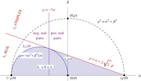
Figure 1: Dependence of $\lambda_{+}$ and $\lambda_{-}$ on $\rho$, $\alpha$ and $\beta$

In general, the roots of $q(x)$ are complicated functions of $\rho,\alpha,\beta,a$ and $t$, but there is a situation where these formulae may be simplified. Let us consider the case where (19) holds and either (20) or (21) holds. This case corresponds to the shaded region of Figure 1. Under these assumptions, $\lambda_{+}\geq 0$ and this allows us to set $a=\lambda_{+}$. Hence $x-\lambda_{+}$ becomes a factor of $q(x)$. Similarly to the substitution made in (18), we may then specify a value of $t$ which forces the remaining cubic polynomial to have the root $\rho+s$ and we may then factor out $x-\rho-s$. Finally, the remaining quadratic may be solved, giving the following result:

Proposition 3.3.

Let the list $(\rho,\alpha+i\beta,\alpha-i\beta,\lambda_{4},\lambda_{5},\ldots,\lambda_{m})$ be realisable, where $\rho$ is the Perron eigenvalue, $\alpha$ is real and $\beta>0$. Assume also that either (20) holds or both (19) and (21) hold. Then for all $s\geq 0$, the list

$$(\rho+s,\mu_{+},\mu_{-},\lambda_{+},\lambda_{4},\lambda_{5},\ldots,\lambda_{m})$$

is realisable, where

$$\mu_{\pm}=\\ \alpha-\frac{s}{2}\pm\frac{1}{2}\sqrt{\frac{s(s-2\alpha)^{2}+\left(s^{2}-4s\alpha-4\beta^{2}\right)\rho+\left(4\beta^{2}+s(3s-4\alpha+4\rho)\right)\lambda_{-}}{\left(s+\rho-\lambda_{-}\right)}}$$

and $\lambda_{+}$ and $\lambda_{-}$ are defined in (17).

Proof.

From the preceding discussion, it suffices to show that (20) implies (19). Indeed

$$\frac{\alpha^{2}+\beta^{2}}{-\alpha}-(\alpha+2\sqrt{2}\beta)=\frac{(\sqrt{2}\alpha+\beta)^{2}}{-\alpha}\geq 0.\qed$$

Example 3.4.

Let $\sigma$ be any list such that

$$\sigma_{0}:=(6,-2+2\sqrt{2}i,-2-2\sqrt{2}i,\sigma)$$

is realisable. Substituting $\rho=6$, $\alpha=-2$ and $\beta=2\sqrt{2}$ in Proposition 3.3, we have that for any $s\geq 0$, the list $\sigma_{1}=(\rho+s,\mu_{-},\mu_{+},0,\sigma)$ is realisable, where

$$\mu_{\pm}:=\frac{1}{2}\left(-4-s\pm\sqrt{16+8s+s^{2}-\frac{288}{6+s}}\right).$$ (22)

In particular, taking $s=2$, we have that $(8,-3,-3,0,\sigma)$ is realisable.

This example is reminiscent of the kind of perturbation given in Theorem 1.4, except that we have also perturbed the imaginary part of the original complex conjugate pair $-2\pm 2\sqrt{2}i$. In fact, using a combination of Proposition 3.3 and Theorem 1.4, it is possible to show that

$$(8,-3+ib,-3-ib,0,\sigma)$$ (23)

is realisable for all $0\leq b\leq 2\sqrt{2}$. To see this, let us label the expression under the square root in (22) as

$$h(s):=16+8s+s^{2}-\frac{288}{6+s}.$$

Since $h(0)=-32\leq-4b^{2}\leq 0=h(2)$ and $h$ is continuous on $[0,2]$, there exists $s_{0}\in[0,2]$ such that $h(s_{0})=-4b^{2}$. Then, taking $s=s_{0}$ gives the realisable list

$$\left(6+s_{0},-2-\frac{s_{0}}{2}+ib,-2-\frac{s_{0}}{2}-ib,0,\sigma\right).$$

Finally, letting $\delta=1-s_{0}/2$ in (1), we may produce (23).

We finish this section with an example for which the limiting eigenvalues $\lambda_{+}$ and $\lambda_{-}$ are complex:

Example 3.5.

Let $\sigma$ be any list for which $\sigma_{0}=(2,i,-i,\sigma)$ is realisable. Applying Theorem 3.1 with $a=0$, $\eta=1$ and $t=1$ produces the realisable spectrum

$$(2.4710\ldots,0.1868\ldots+(0.6666\ldots)i,0.1868\ldots-(0.6666\ldots)i,-0.8445\ldots,\sigma).$$

$t=5$ gives

$$(3.8755\ldots,0.4100\ldots+(0.5573\ldots)i,0.4100\ldots-(0.5573\ldots)i,-2.6954\ldots,\sigma).$$

$t=500$ gives

$$(32.1356\ldots,0.499\ldots+(0.5007\ldots)i,0.499\ldots-(0.5007\ldots)i,-31.1336\ldots,\sigma),$$

illustrating the convergence of two of the eigenvalues of $\sigma_{1}$ to $\lambda_{\pm}=1/2\pm(1/2)i$.

References

[1]
Anthony Cronin.
Characterizing the Spectra of Nonnegative Matrices.
PhD thesis, School of Mathematical Sciences, University College
Dublin, 2012.
[2]
Shmuel Friedland.
On an inverse problem for nonnegative and eventually nonnegative
matrices.
Israel Journal of Mathematics, 29(1):43–60, 1978.
[3]
Siwen Guo and Wuwen Guo.
Perturbing non-real eigenvalues of non-negative real matrices.
Linear Algebra and its Applications, 426(1):199 – 203, 2007.
[4]
Wuwen Guo.
Elgenvalues of nonnegative matrices.
Linear Algebra and its Applications, 266(0):261 – 270, 1997.
[5]
Charles R. Johnson.
Row stochastic matrices similar to doubly stochastic matrices.
Linear and Multilinear Algebra, 10(2):113–130, 1981.
[6]
Thomas J. Laffey.
Perturbing non-real eigenvalues of nonnegative real matrices.
ELA. The Electronic Journal of Linear Algebra [electronic
only], 12:73–76, 2004.
[7]
Thomas J. Laffey and Eleanor Meehan.
A characterization of trace zero nonnegative matrices.
Linear Algebra and its Applications, 302/303(0):295 – 302,
1999.
[8]
Thomas J. Laffey and Helena Šmigoc.
Nonnegative realization of spectra having negative real parts.
Linear Algebra and its Applications, 416(1):148 – 159, 2006.
(Special Issue devoted to the Haifa 2005 conference on matrix
theory).
[9]
Thomas J. Laffey and Helena Šmigoc.
Structured matrices in the nonnegative inverse eigenvalue problem.
In Mathematical Papers in Honor of Eduardo Marques de Sá,
volume 39. Textos de Matemática, 2007.
[10]
Raphael Loewy and David London.
A note on an inverse problem for nonnegative matrices.
Linear and Multilinear Algebra, 6(1):83–90, 1978.
[11]
Helena Šmigoc.
The inverse eigenvalue problem for nonnegative matrices.
Linear Algebra and its Applications, 393(0):365 – 374, 2004.
(Special Issue on Positivity in Linear Algebra).
[12]
Helena Šmigoc.
Construction of nonnegative matrices and the inverse eigenvalue
problem.
Linear and Multilinear Algebra, 53(2):85–96, 2005.