Boundary rigidity with partial data
Abstract.
We study the boundary rigidity problem with partial data consisting of determining locally the Riemannian metric of a Riemannian manifold with boundary from the distance function measured at pairs of points near a fixed point on the boundary. We show that one can recover uniquely and in a stable way a conformal factor near a strictly convex point where we have the information. In particular, this implies that we can determine locally the isotropic sound speed of a medium by measuring the travel times of waves joining points close to a convex point on the boundary.
The local results lead to a global lens rigidity uniqueness and stability result assuming that the manifold is foliated by strictly convex hypersurfaces.
1. Introduction and main results
Travel time tomography deals with the problem of determining the sound speed or index of refraction of a medium by measuring the travel times of waves going through the medium. This type of inverse problem, also called the inverse kinematic problem, arose in geophysics in an attempt to determine the substructure of the Earth by measuring the travel times of seismic waves at the surface. We consider an anisotropic index of refraction, i.e., a sound speed depending on the direction. The Earth is generally isotropic. However, more recently it has been realized, by measuring these travel times, that the inner core of the Earth exhibits anisotropic behavior with the fast direction parallel to the Earth’s spin axis, see [5]. In the human body, muscle tissue is anisotropic. As a model of anisotropy, we consider a Riemannian metric . The problem is to determine the metric from the lengths of geodesics joining points on the boundary.
This leads to the general question of whether given a compact Riemannian manifold with boundary one can determine the Riemannian metric in the interior knowing the boundary distance function joining points on the boundary , with . This is known as the boundary rigidity problem. Of course, isometries preserve distance, so that the boundary rigidity problem is whether two metrics that have the same boundary distance function are the same up to isometry fixing the boundary. Examples can be given of manifolds that are not boundary rigid. Such examples show that the boundary rigidity problem should be considered under some restrictions on the geometry of the manifold. The most usual of such restrictions is simplicity of the metric. A Riemannian manifold (or the metric ) is called simple if the boundary is strictly convex (positive second fundamental form) and any two points are joined by a unique minimizing geodesic. Michel conjectured [21] that every simple compact Riemannian manifold with boundary is boundary rigid.
Simple surfaces with boundary are boundary rigid [29]. In higher dimensions, simple Riemannian manifolds with boundary are boundary rigid under some a-priori constant curvature on the manifold or special symmetries [2], [13]. Several local results near the Euclidean metric are known [39], [19], [3]. The most general result in this direction is the generic local (with respect to the metric) one proven in [41]. Surveys of some of the results can be found in [16], [42], [8].
In this paper, we consider the boundary rigidity problem in the class of metrics conformal to a given one and with partial (local) data, that is, we know the boundary distance function for points on the boundary near a given point. Partial data problems arise naturally in applications since in many cases one doesn’t have access to the whole boundary. We prove the first result on the determination of the conformal factor locally near the boundary from partial data without assuming analyticity. We develop a novel method to attack partial data non-linear problems that will likely have other applications.
We now describe the known results with full data on the boundary. Let us fix the metric and let be a positive smooth function on the compact manifold with boundary . The problem is whether we can determine from Notice that in this case the problem is not invariant under changes of variables that are the identity at the boundary so that we expect to be able to recover under appropriate a-priori conditions. This was proven by Mukhometov in two dimensions [23], and in [24] in higher dimensions for the case of simple metrics. Of particular importance in applications is the case of an isotropic sound speed that is when we are in a bounded domain of Euclidean space and is the Euclidean metric. This is the isotropic case. This problem was considered by Herglotz [14] and Wieckert and Zoeppritz [51] for the case of a spherical symmetric sound speed. They found a formula to recover the sound speed from the boundary distance function assuming . Notice that this condition is equivalent to the existence of a strictly convex foliation and is more general than simplicity, see Section 6.
From now on we will call the function . Below, is related to .
The partial data problem, that we will also call the local boundary rigidity problem111It is local in the sense that is known locally and depends on locally; the term local has been used before to indicate that the metric is a priori close to a fixed one., in this case is whether knowledge of the distance function on part of the boundary determines the sound speed locally. Given another smooth , here and below we define , and in the same way but related to . We prove the following uniqueness result:
Theorem 1.1.
Let , let , be smooth and let be strictly convex with respect to both and near a fixed . Let for , on near . Then in near .
As mentioned earlier, this is the only known result for the boundary rigidity problem with partial data except in the case that the metrics are assumed to be real-analytic [19]. The latter follows from determination of the jet of the metric at a convex point from the distance function known near
The boundary rigidity problem is closely connected to the lens rigidity one. To define the latter, we first introduce the manifolds , defined as the sets of all vectors with , unit in the metric , and pointing outside/inside . We define the scattering relation
| (1) |
in the following way: for each , , where are the exit point and direction, if exist, of the maximal unit speed geodesic in the metric , issued from . Let
be its length, possibly infinite. If , we call non-trapping. The maps together are called lens relation (or lens data).
The lens rigidity problem is whether the scattering relation (and possibly, ) determine (and the topology of ) up to an isometry as above. The lens rigidity problem with partial data for a sound speed is whether we can determine the speed near some from known near the unit sphere considered as a subset of , i.e., for vectors with base points close to and directions pointing into close to ones tangent to . For general metrics, we want to recover isometric copies of the metrics locally, as above.
We assume that is strictly convex at w.r.t. . Then the boundary rigidity and the lens rigidity problems with partial data are equivalent: knowing near is equivalent to knowing in some neighborhood of . The size of that neighborhood however depends on a priori bounds of the derivatives of the metrics with which we work. This equivalence was first noted by Michel [21], since the tangential gradients of on give us the tangential projections of and , see also [38, sec. 2]. Note that local knowledge of is not needed for the lens rigidity problem222If is given only, then the problem is called scattering rigidity in some works, and in fact, can be recovered locally from either or , see for example the proof of Theorem 5.2.
Vargo [50] proved that real-analytic manifolds satisfying an additional mild condition are lens rigid. Croke has shown that if a manifold is lens rigid, a finite quotient of it is also lens rigid [8]. He has also shown that the torus is lens rigid [4]. G. Uhlmann and P. Stefanov have shown lens rigidity locally near a generic class of non-simple manifolds [44]. In a recent work, Guillarmou [12] proved that in two dimensions, one can determine from the lens relation the conformal class of the metric if the trapped set is hyperbolic and there are no conjugate points. He also proved deformation lens rigidity in higher dimensions under the same assumptions. The only result we know for the lens rigidity problem with incomplete (but not local) data is for real-analytic metric and metric close to them satisfying the micolocal condition in the next sentence [44]. While in [44], the lens relation is assumed to be known on a subset only, the geodesics issued from that subset cover the whole manifold and their conormal bundle is required to cover . In contrast, in this paper, we have localized information.
We state below an immediate corollary of our main result for this problem. For the partial data problem instead of assuming locally, we can assume that in a neighborhood of . To reduce this problem to Theorem 1.1 directly, we need to assume first that on near to make the definition of independent of the choice of the speed but in fact, one can redefine the lens relation in a way to remove that assumption, see [44].
Theorem 1.2.
Let , , be as in Theorem 1.1 with on near . Let near . Then in near .
Remark 1.1.
The theorem or its corollary does not preclude the existence of an infinite set of speeds all having the same boundary distance function (or lens data) in , where is some fixed small set but not coinciding in any fixed neighborhood of . In principle, this may happen when the maximal neighborhood of , which can be covered with strictly convex surfaces, which continuously deform , shrinks when . Then the theorem does not imply existence of a fixed neighborhood of , where all speeds are equal. If one assumes that a priori, the sound speeds have uniformly bounded derivatives of some finite order near , this situation does not arise, and this case is covered by Theorem 5.2 below.
The linearization of the boundary rigidity and lens rigidity problem is the tensor tomography problem, i.e., recovery of a tensor field up to “potential fields” from integrals along geodesics joining points on the boundary. It has been extensively studied in the literature for both simple and non-simple manifolds [22, 11, 26, 27, 28, 30, 32, 34, 36, 40, 43, 46, 1]. See the book [33] and [28] for a recent survey. The local tensor tomography problem has been considered in [17] for functions and real-analytic metrics and in [18] for tensors of order two and real-analytic metrics. Those results can also be thought of as support theorems of Helgason type. The only known results for the local problem for smooth metrics and integrals of functions is [49].
Now we use a layer stripping type argument to obtain a global result which is different from Mukhometov’s for simple manifolds.
Definition 1.1.
Let be a compact Riemannian manifold with boundary. We say that satisfies the foliation condition by strictly convex hypersurfaces if is equipped with a smooth function which level sets , with some are strictly convex viewed from for , is non-zero on these level sets, and and has empty interior.
The statement of the global result on lens rigidity is as follows:
Theorem 1.3.
Let , let , be smooth and equal on , let be strictly convex with respect to both and . Assume that can be foliated by strictly convex hypersurfaces for . Then if on , we have in .
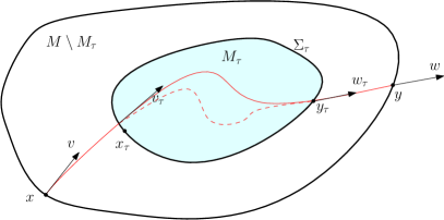
A more general foliation condition under which the theorem would still hold is formulated in [45], see also Definition 5.1 below. In particular, does not need to be and one can have several such foliations with the property that the closure of their union is . If we can foliate only some connected neighborhood of , we would get there. Next, it is enough to require that is simple (or that it is included in a simple submanifold), see the proof of Theorem 1.3 and Figure 2, to prove in first, and then use Mukhometov’s results to complete the proof. The class of manifolds we get in this way is larger than the simple ones, and can have conjugate points.
Speeds not necessarily radial (with the Euclidean metric) under the condition considered by Herglotz and Wieckert and Zoeppritz satisfy the foliation condition of the theorem, see also Section 6. Other examples of non-simple metrics that satisfy the condition are the tubular neighborhood of a closed geodesic in negative curvature. These have trapped geodesics. It follows from the result of [31], that manifolds with no focal points satisfy the foliation condition. It would be interesting to know whether this is also the case for simple manifolds. As it was mentioned earlier, manifolds satisfying the foliation condition are not necessarily simple.
The linearization of the non-linear problem with partial data considered in Theorem 1.1 was considered in [49], where uniqueness and stability were shown. This corresponds to integrating functions along geodesics joining points in a neighborhood of . The method of proof of Theorem 1.1 relies on using an identity proven in [39] to reduce the problem to a ”pseudo-linear” one: to show uniqueness when one integrates the function and its derivatives on the geodesics for the metric joining points near , with weight depending non-linearly on both and . Notice that this is not a proof by linearization, and unlike the problem with full data, an attempt to do such a proof by linearization is connected with essential difficulties. The proof of uniqueness for this linear transform follows the method of [49] introducing an artificial boundary and using Melrose’ scattering calculus. In section 2, we do the reduction to a “pseudo-linear problem”, and in section 3, we show uniqueness for the ”pseudo-linear” problem. In section 4, we finish the proofs of the main theorems.
We also prove Hölder conditional stability estimates related to the uniqueness theorems above. In case of data on the whole boundary, such an estimate was proved in [41, section 7] for simple manifolds and metrics not necessarily conformal to each other. Below, the norm is defined in a fixed coordinate system. The next theorem is a local stability result, corresponding to the local uniqueness result in Theorem 1.1.
Theorem 1.4.
There exists and with the following property. For any , , and , there exists and with the property that for any two positive , with
| (2) |
and for any neighborhood of on , we have the stability estimate
| (3) |
for some neighborhood of in .
In Theorem 5.2, we prove a Hölder conditional stability estimates of global type as well, which can be considered as a “stable version” of Theorem 1.3.
The plan of the paper is as follows. The reduction to a pseudo-linear problem is done in Section 2. In Section 3, we present linear analysis using the scattering calculus. The main result there is Proposition 3.3, which is of its own interest as well. The proofs of the three uniqueness theorems are in Section 4. In Section 5, we prove the local stability result in Theorem 1.4 and the global Theorem 5.2. As an application of our results, we revisit the class of speeds studied by Herglotz [14] and Wieckert & Zoeppritz [51] in Section 6 without assuming that they are radial and we prove that they are lens rigid. In particular, we show that their condition (59) is equivalent to the requirement that the Euclidean spheres are strictly convex for the metric ; therefore, it is a foliation condition.
Acknowledgments. We would like to thank Christopher Croke for pointing out an error in the formulation of Theorem 1.3 in an earlier version of the paper and for helpful comments.
2. Reducing the non-linear problem to a pseudo-linear one
We recall the known fact [19] that one can determine the jet of at any boundary point at which is convex (not necessarily strictly) from the distance function known near . For a more general result not requiring convexity, see [44]. Since the result in [19] is formulated for general metrics, and the reconstruction of the jet is in boundary normal coordinates, we repeat the proof in this (simpler) situation of recovery a conformal factor. As in [19], we say that is convex near , if for any two distinct points , close enough to , there exists a geodesic joining them such that its length is and all the interior of belongs to the interior of . Of course, strict convexity (positive second fundamental form at ) implies convexity.
Lemma 2.1.
Let and be smooth and let be convex at with respect to and . Let near . Then on near for any multiindex .
Proof.
Let be a neighborhood of on such that for any , we have the property guaranteeing convexity at . Let be a boundary normal coordinate related to ; i.e., , and in . We can complete to a local coordinate system , where parameterizes near .
It is enough to prove
| (4) |
For , this follows easily by taking the limit in , ; and this can be done for any . Let be the first value of for which (4) fails. Without loss of generality, we may assume that it fails at , and at . Then in , . Consider the Taylor expansion of w.r.t. with close enough to . We get in some neighborhood of in minus the boundary.
Now, let be a minimizing geodesic in the metric connecting and when as well, close enough to , see also [19]. Let be the geodesic ray transform of the tensor field defined as an integral of along . All geodesics here are parameterized by a parameter in rather than being unit speed, and therefore the transform is parameterized differently than usual one. Then by what we proved above. On the other hand,
because minimizes integrals of along curves connecting and . This a contradiction. ∎
The starting point is an identity in [39]. We will repeat the proof.
Let , be two vector fields on a manifold (which will be replaced later with ). Denote by the solution of , , and we use the same notation for with the corresponding solution are denoted by . Then we have the following simple statement.
Lemma 2.2.
For any and any initial condition , if and exist on the interval , then
| (5) |
Proof.
Set
Then
The proof of the lemma would be complete by the fundamental theorem of calculus
if we show the following
| (6) |
Indeed, (6) follows from
after setting , . ∎
Let , be two speeds. Then the corresponding metrics are , and . The corresponding Hamiltonians and Hamiltonian vector fields are
and the same ones related to . We used the notation .
We change the notation at this point. We denote points in the phase space , in a fixed coordinate system, by . We denote the bicharacteristic with initial point by .
Then we get the identity already used in [39]
| (7) |
We can naturally think of the scattering relation and the travel time as functions on the cotangent bundle instead of the tangent one. Then we get the following.
Proposition 2.1.
Assume
| (8) |
for some . Then
2.1. Linearization near and Euclidean
As a simple exercise, let , and linearize for near first under the assumption that outside an open region . Then
| (9) |
and we get the following formal linearization of (7)
| (10) |
where
| (11) |
Notice that we would get the same thing if we replace in (7) by . We integrate over the whole line because the integrand vanishes outside the interval . The last components of (10) imply
| (12) |
Now, assume that this holds for all . Then , and since on , we get .
2.2. The general case
We take the second -dimensional component on (7) and use the fact that on the bicharacteristics related to . We assume that both geodesics extend to . We want to emphasize that the bicharacteristics on the energy level , related to , do not necessarily stay on the same energy level for the Hamiltonian . We get
| (13) |
for any for which (8) holds. As before, we integrate over because the support of the integrand vanishes for (for that, we extend the bicharacteristics formally outside so that they do not come back ). Write
to get
| (14) |
One of terms on the r.h.s. above involves which equals on the bicharacteristics of on the level .
Introduce the exit times defined as the minimal (and the only) so that . They are well defined near , if is strictly convex at . We need to write as a function of . We have
Then we get, with as in (11),
| (15) |
for any bicharacteristic (related to the speed ) in our set, where
| (16) |
A major inconvenience with this representation is that the exit time function (recall that we assume strong convexity) becomes singular at . More precisely, the normal derivative w.r.t. when is tangent to has a square root type of singularity. On the other hand, we have some freedom to extend the flow outside since we know that the jets of and at are the same near : therefore, any smooth local extension of is also a smooth extension of . Then for any close enough to , the bicharacteristics originating from it will be identical once they exit but are still close enough to it. Similarly, instead of starting from , we could start at points and codirections close to it, but away from .
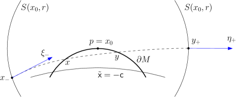
With this in mind, we push the boundary away a bit. Let represent the point near which we work, in a fixed coordinate system. Extend smoothly near . Let be the sphere in the metric centered at with radius . For with in the geodesic ball , redefine to be the travel time from to . Let be the set of all points on and incoming unit directions so that the corresponding geodesic in the metric is close enough to one tangent to at . Similarly, let be the set of such pairs with outgoing directions. Redefine the scattering relation locally to act from to , and redefine similarly, see Figure 1. Then under the assumptions of Theorem 1.2, and on . We can apply the construction above by replacing locally by . The advantage we have now is that on , the travel time is non-singular. Equalities (15), (16) are preserved then.
We now have
| (17) |
Then by the strict convexity,
| (18) |
2.3. A new linear problem
The arguments above lead to the following linear problem:
Problem. Assume (15) holds with some supported in , for all geodesics close to the ones originating from (i.e. initial point and all unit initial co-directions tangent to ). Assume that is strictly convex at w.r.t. the speed . Assume (18). Is it true that near ?
We show below in Proposition 3.3, that the answer is affirmative. Note that this reduces the original non-linear problem to a linear one but this is not a linearization. Then Theorem 1.2 follows from it. On the other hand, Theorem 1.2 is not equivalent to that problem because the weight there has a specific structure, thus Proposition 3.3 is a more general statement.
3. Linear analysis
We first recall the setting introduced in [49] in our current notation. There the scalar X-ray transform along geodesics was considered, namely for ,
where is the geodesic with lift to having starting point . Here is assumed to have a strictly convex boundary, which can be phrased as the statement that if is a defining function for , then whenever . One then considers a point , and another function , denoted in [49] by , such that , , and the level sets of near the are strictly concave when viewed from the superlevel sets (which are on the side of when talking about the -level set with ), i.e. if , namely if . For , we denote by ; we assume that is such that is compact on , and the concavity assumption holds on . Then it was shown that the X-ray transform restricted to such that leaves with both endpoints on (i.e. at ) is injective if is sufficiently small, and indeed one has a stability estimate for in terms of on exponentially weighted spaces.
To explain this in detail, let be the boundary defining function of the artificial boundary, , that we introduced; indeed it is convenient to work in , a manifold extending across the boundary, extending to smoothly, and defining as the extension of , so is a smooth manifold with boundary, with only the artificial boundary being a boundary face. Then one writes relative to a product decomposition of near . The concavity condition becomes that for whose -component vanishes,
with a new , see the discussion preceding Equation (3.1) in [49]. For , , , one considers the map
defined for a function on . This differs from [49] in that the weight differs by from the weight used in [49]; this simply has the effect of removing an in [49, Proposition 3.3], as compared to the proposition stated below. If is sufficiently small, or instead has sufficiently small support, for , only integrates over points in such that leaves with both endpoints on , i.e. over corresponding to -local geodesics – the set of the latter is denoted by . We refer to the discussion around [49, Equation (3.1)] for more detail, but roughly speaking the concavity of the level sets of means that the geodesics that are close to being tangent to the foliation, with ‘close’ measured by the distance from the artificial boundary, , then they cannot reach (or reach again, in case they start there) without reaching for some fixed ; notice that the geodesics involved in the integration through a point on the level set make an angle with the tangent space of the level set due to the compact support of . Then we consider the map . The main technical result of [49], whose notation involving the so-called scattering Sobolev spaces and scattering pseudodifferential operators is explained below, was:
Proposition 3.1.
Further, if is sufficiently small, then for suitable choice of with , , is elliptic in on a neighborhood of .
Shrinking further if needed, satisfies the estimate
| (19) |
for supported in .
We now briefly explain the role of the so-called scattering pseudodifferential operators and the corresponding Sobolev spaces (which are typically used to study phenomena ‘at infinity’) in our problem (where there is no obvious ‘infinity’); we refer to [49, Section 2] for a more thorough exposition. These concepts were introduced by Melrose, [20], in a general geometric setting, but on these operators actually correspond to a special case of Hörmander’s Weyl calculus [15], also studied earlier by Shubin [37] and Parenti [25]. So consider the reciprocal spherical coordinate map, , with (unit sphere), and map . This map is a diffeomorphism onto its range, and it provides a compactification of (the so called radial or geodesic compactification) by adding as infinity to , to obtain , which is now diffeomorphic to a ball. Now for general above, we may regard, at least locally333That is, possibly at the cost of shrinking it; in fact all concepts below are essentially local within , thus even in full generality one can reduce scattering objects to (conic regions near infinity in) this way, much as standard Sobolev spaces and pseudodifferential operators are so reduceable to subsets of with compact closure also as a coordinate chart in , and thus obtain an identification of with a region intersection , thus our artificial boundary corresponds to infinity at . In particular, notions from can now be transferred to a neighborhood of our artificial boundary. Since the relevant vector fields on are generated by translation invariant vector fields, which are complete under the exponential map, the transferred analysis replaces the incomplete geometry of standard vector fields on by a complete one. Concretely, these vector fields, when transferred, become linear combinations of and , with smooth coefficients. In particular, these are the vector fields with respect to which Sobolev regularity is measured. Thus, is the so-called scattering Sobolev space, which is locally, under the above identification, just the standard weighted Sobolev space , see [49, Section 2], while is Melrose’s scattering pseudodifferential algebra, which locally, again under this identification, simply corresponds to quantizing symbols with on , see again [49, Section 2] for more detail. Note that ellipticity in this algebra, called full ellipticity, is both in the sense as and , i.e. modulo symbols one order lower and with an extra order of decay as .
Notice that (19) implies the estimate
for the unconjugated operator, valid when is supported in . Rewriting as , this gives that for , ,
see the discussion in [49] after Lemma 3.6.
After this recollection, we continue by generalizing (15) to regard the functions and entering into it as independent unknowns, while restricting the transform to the region of interest . So let be defined by
where is the geodesic with lift to having starting point . Let . This is a vector valued version of the geodesic X-ray transform considered in [49], and described above, sending functions on with values in to functions with values in . We then define as a map from -valued functions on to valued functions on by
as in [49]; this is a diagonal operator: . Then we consider the map , and in addition to the properties mentioned above in the scalar setting, we are also interested in continuity properties in terms of the background data, such as in the background metric as well as the function . Recall that the map
| (20) |
is a local diffeomorphism, and similarly for in which takes the place of ; see the discussion around [49, Equation (3.2)-(3.3)]; indeed this is true for more general curve families. Here is the blow-up of at the diagonal , which essentially means the introduction of spherical/polar coordinates, or often more conveniently projective coordinates, about it. Concretely, writing the (local) coordinates from the two factors of as ,
| (21) |
give (local) coordinates on this space. Note that when are given by geodesics of a metric just -near a fixed background metric , as maps, depend continuously on in the topology.
In order to consider continuity properties in in a -neighborhood of a fixed function , it is convenient to use the map to identify a neighborhood of with a neighborhood of the origin in . Thus, for fixed, but being -close to , on this fixed background , the pulled pack metrics depend continuously on as maps ; this normalizes to be simply the first coordinate function on . Correspondingly, below, the continuous dependence, of all objects discussed, on (in the topology) is automatic: what is meant always is that by pull-back to the resulting objects, living on fixed domains such as , depend continuously on and , which follows from the continuous dependence of these objects on . Since we do not want to overburden the notation, we do not write this pull-back explicitly.
The main technical result here is:
Proposition 3.2.
For , let
Then , and the map is continuous from the topology to the Fréchet topology of .
Further, if is sufficiently small and (18) holds, then for suitable choice of with , , if we write , with corresponding to the first component, the last components, in the domain space, then is elliptic in in a neighborhood of .
Remark 3.1.
Notice that ellipticity being an open condition, this means that there exists such that if , then the same works for all -close to .
Further, in view of the paragraph preceding the proposition, the map is continuous from the topology to the Fréchet topology of , where the latter is understood to actually stand for via the identifications discussed above.
Proof.
This is simply a vector valued version of [49, Proposition 3.3] and [49, Lemma 3.6], recalled above in Proposition 3.1. In particular, to show , it suffices to show that is a matrix of pseudodifferential operators , , , depending continously on . But for , with being completely analogous, has the form
The only difference from [49, Proposition 3.3] then is the presence of the weight factor
It is convenient to rewrite this via the metric identification, say by , in terms of tangent vectors. Changing the notation for the flow, in our coordinates , writing now
for the lifted geodesic ,
replaces As in [49, Proposition 3.3] one rewrites the integral in terms of coordinates on the left and right factors of (i.e. one explicitly expresses the Schwartz kernel), using that the map of (20) is a local diffeomorphism, and similarly for ; we again refer to the discussion around [49, Equation (3.2)-(3.3)]. Further,
is a smooth map (depending continuously on in the respective topologies) so composing it with from the right, one can re-express the integral giving away from the boundary as
as in [49, Equation (3.7)], with a smooth function of the indicated variables (thus smooth on ), depending continuously on in the respective topologies, and with
with , bounded below by a positive constant, a weight factor, and where is written as . Recall from [49, Section 2] that coordinates on Melrose’s scattering double space, on which the Schwartz kernels of elements of are conormal to the diagonal, near the lifted scattering diagonal, are (with )
Further, it is convenient to write coordinates on in the region of interest (see the beginning of the paragraph of Equation (3.10) in [49]), namely (the lift of) , as
with the norms being Euclidean norms,444This is an example of partial projective coordinates for a blow-up. instead of (21); we write in terms of these. Note that these are . Then, similarly, near the boundary as in [49, Equation (3.13)], one obtains the Schwartz kernel
| (22) | ||||
with the density factor smooth, positive, depending continuously on in the respective topologies, at . Here
are valid coordinates on the blow-up of the scattering diagonal in555This is another example of partial projective coordinates for a blow-up. , , which is the case automatically on the support of the kernel due to the argument of , cf. the discussion after [49, Equation(3.12)], so the argument of is smooth on this blown up space still depending continuously on in the respective topologies. We can evaluate this argument: for instance, by [49, Equation(3.10)],
with smooth, while the subsequent equation in the same location gives
with smooth; here both and depend continuously on in the respective topologies. This proves the first part of the proposition as in [49, Proposition 3.3].
To prove the second part, note that in view of (22) (which just needs to be evaluated at ), [49, Lemma 3.5] is replaced by the statement that the boundary principal symbol of in is twice the -Fourier transform of
| (23) |
while for it is twice the -Fourier transform of
with defined analogously to . (Recall that is the component of , and the convexity assumption on is that is positive; see [49] above Equation (3.1).) For , see (18), the invertibility of the principal symbol, with values in matrices, of the principal symbol of follows when is chosen as in [49, Lemma 3.6], for it is times the boundary symbol in [49, Lemma 3.6] times the identity matrix. In general, due to the perturbation stability of the property of invertibility, the same follows for sufficiently small. ∎
Corollary 3.1.
With the notation of Proposition 3.2, there is such that if , then satisfies the estimate
| (24) |
for supported in , with the constant uniform in . Further, fixing , there exist and and such that can be taken uniform for -close to a reference in , and the estimate holds even for supported in (in place of ).
Remark 3.2.
As in the case of the preceding proposition, the dependence on is also continuous, i.e. by possibly increasing , can be taken uniform for -close to a reference and -close to a reference .
Proof.
By the density of elements of in supported in , it suffices to consider to prove (24).
Consider , . Let be elliptic and invertible (one can e.g. locally identify with ; then on the Fourier transform side multiplication by works). Thus, , with acting diagonally on , is in , depending continuously, in the Fréchet topology of pseudodifferential operators, on in , and is elliptic in locally in a neighborhood of . This implies, as presented in [49] after Lemma 3.6 (without the uniform discussion on ), relying on the arguments at the end of Section 2 there, that there exist and such that if is -close to in , then if is sufficiently small then satisfies
| (25) |
for supported in . Here is the space relative to a non-degenerate scattering density — the latter are equivalent to the lifted Lebesgue measure from , thus are bounded multiples of .
We recall the essential part of this argument briefly. One considers the whole family of domains , which can be identified with each other locally in the region of interest by the maps , i.e. simply translation in the -coordinate, so instead of considering a family of spaces with an operator on each of them, one can consider a fixed space, denote this by , with a continuous (in ) family of operators, , namely ; these depend continuously on in the Fréchet sense discussed above. Notice that we are interested in the region666If we are interested in the region , , within , with to be specified, we take e.g. in the discussion below, and the desired continuous with , and in this case with on , still exists. , and that there is a continuous function on with and on . Correspondingly, in the translated space, on the image of ; notice that this region shrinks as goes to . On the other hand, there is a fixed open set , a neighborhood of , on which the operators are elliptic in for . Let be a compact subset of , still including a neighborhood of , be identically on a neighborhood of . Then the elliptic parametrix construction (which is local, and uniform in by the continuity) produces a parametrix family , , where only, but , uniformly in , depending continuously on in the Fréchet topologies. Then (multiplying the parametrix identity by from left and right and applying to ) for supported in , . Now, the Schwartz kernel of is Schwartz, i.e. is bounded by for any , uniformly in . (Here we write, say, the Schwartz kernel relative to scattering densities, but as is arbitrary, this makes little difference.) For , let be supported, say, in , identically near the region ; one may assume that on by making small. Then, by Schur’s lemma, , acting say on (i.e. the -space relative to scattering densities) is bounded by for any . Thus, there is such that is invertible for on . (Notice here that this requires the smallness of a seminorm of in the Fréchet topology of pseudodifferential operators; the continuity discussed above means that that this requires the -closeness of to for some .) In particular, for supported in , so , , so inverting the factor on the left and then undoing the transformation gives the desired conclusion (25).
Thus, with , we have, with all norms being -norms,
By (25), , . On the other hand, , as elements of are -bounded. (By the continuity of the map from to in the appropriate Fréchet topologies, again there is such that is uniform when is -close to .) Using the Cauchy-Schwartz inequality, for ,
Thus, the last three terms are bounded by in absolute value, so we conclude that, with ,
| (26) |
completing the proof of the corollary if .
The general case follows via conjugating by an elliptic, invertible, element of , which is thus an isomorphism from to . Note that such a conjugation does not change the principal symbol, thus the ellipticity. ∎
We now remark that the even simpler setting of the scalar transform with a positive weight on , , which was not considered in [49], and which can be considered a special case of with simply replaced by . Thus, for consistency with the above notation, let be the weight on induced by the metric identification, and let
Then the above argument gives that . If at , the weight is independent of the momentum variable , it further gives that is elliptic in a neighborhood of . More generally, a modification of the argument of [49] due to H. Zhou [52] allows one to show that the principal symbol is fully elliptic in in the scattering sense merely assuming that is positive (but not the independence condition just mentioned). To see this, one has to Fourier transform (23) in with replaced by . The -Fourier transform is unaffected by the presence of , and gives, as in [49, Equation (3.16)],
Replacing with a Gaussian, , , which does not have compact support, but an approximation argument (in symbols of order ) will give this desired property, one can compute that this is, up to a constant factor,
We need to compute the Fourier transform in . Following [52], one expresses this in polar coordinates in :
which in turn becomes, up to a constant factor,
The integrand is now positive, which gives the desired ellipticity at . (One also needs to check the ellipticity as ; this is standard, see [49, 52].) One proceeds with an approximation argument as in [49, 52] to complete the proof of the ellipticity. Thus, the above argument gives the estimate
As discussed in [49] after Lemma 3.6, this yields the following corollary:
Corollary 3.2.
The weighted scalar transform with a positive weight on , with the associated weight on ,
satisfies that for there is such that for , , , we have
We now return to the actual case of interest and apply Corollary 3.1 with , . If we show that (uniformly in , which are indeed irrelevant for this argument) given there is such that , i.e. is bounded by a small multiple of a derivative of times in , when is supported in , , then for sufficiently small (24) proves that if vanishes, then so does , i.e. in this case so does , for the term can then be absorbed into the left hand side of (24):
| (27) |
Further, rewriting this by removing the weights , and estimating the norms in terms if the standard -based space, cf. the discussion after [49, Lemma 3.6] already referenced above,777The loss is actually just the loss of a power of , due to change of the measure. gives, for ,
| (28) |
with uniform for -close to .
But this can now be easily done: let be a smooth vector field with , so is tangent to the boundary of for every , and make the non-degeneracy assumption that, for some , there is a continuous such that and the -flow takes every point in to in time (i.e. outside the original manifold). Then the Poincaré inequality for gives888Notice that our treatment of the -dependence of the problem relies on reducing to a model, where is replaced by a fixed function , so the following argument is in fact uniform in .
| (29) |
for vanishing outside , hence the constant is small if is small. (Here the space we need is the scattering -space, , which is times the standard -space, but the extra weight does not affect the argument, since commutes with multiplication by powers of .)
To see (29), we recall a standard proof of the local Poincaré inequality: in order to reduce confusion with the notation, let be the coordinates, being the boundary of (so would be ), and assume that the flow of flows from every point in to outside the region in ‘time’ . To normalize the argument, assume that in , and we want to estimate in . We assume that the space is given by a density . Then, for , , with support in , by the fundamental theorem of calculus and the Cauchy-Schwartz inequality,
Squaring both sides, multiplying by , and integrating in (to ) gives
This says that actually
proving the claim (using ) in view of the quasi-isometry invariance (which gives a constant factor) of the bound (29). Even if there is more complicated topology, so there are no global coordinates and vector fields as stated, dividing up the problem into local pieces and adding them together gives the desired result: taking steps of size , one needs steps to cover the set, using cutoff functions to localize is easily seen to give a bound proportional to .
On the other hand, in view of the strict convexity of the boundary, one can construct such a and . With , this is exactly the desired conclusion since , namely (27), and thus (28), hold.
In fact, we can prove the analogue of (27) on stronger spaces:
| (30) |
which in turn gives, for ,
| (31) |
with uniform for -close to . To see this, notice that (24) is an elliptic estimate when we have , , for
implies that999Notice that the scattering derivatives are actually weaker than the derivatives entering , and one can absorb the term given by commuting a scattering derivative through into the last term on the right hand side.
For , , we have the second term on the right hand side controlled by in in view of (27), so the -norm of is in fact controlled by , which we can iterate further101010We can easily allow non-integer by slightly modifying the argument here. to prove (30).
In summary we have proved that with the standard -space now (as the exponential weight maps such to , see also the discussion after Lemma 3.6 in [49]):
Proposition 3.3.
There is such that for , if and , then .
In fact, for , , there exist , and such that the following holds. For there is such that if , is -close to in , is -close to in , then
Moreover, with , and being defined analgously to with being replaced by , we have: for and there exist , , and such that the following holds. For there is such that if , is -close to in , is -close to in , then implies that
4. Proof of Theorems 1.1-1.3
Proof of Theorem 1.2.
Let and be as in the theorem. Redefine the scattering relation as in Figure 1. By Proposition 2.1, we get , see (15) for all geodesics close enough to the ones tangent to at . The weights are given by (17), in the new parameterization, with the ellipticity condition satisfied by (18). Then Proposition 3.3 implies in a neighborhood of , where as in (11). ∎
Proof of Theorem 1.1.
Note first that we can complete , and similarly to compact Riemannian manifolds without boundary. Then we can choose a neighborhood of small enough so that the exponential map based on any point of that neighborhood is a local diffeomorphism for short enough vectors, both for and for . This implies that there is a neighborhood of so that the distance between any two points , in is realized by , related to the first and the second metric, respectively, where is the localized exponential map as above. We can easily recover and on by taking the limit . As Michel proved [21], for simple manifolds, the scattering elation can be recovered by differentiating the distance function, see also [38, sec. 2]. This applies to our case as well because if is small enough. Then the proof follows from Theorem 1.2. ∎
Proof of Theorem 1.3.
Theorem 1.3 is now an easy consequence of Theorem 1.1 using a layer stripping argument. Let . Assume , then has non-empty interior. On the other hand, let ; if we are done, for then . Thus, suppose , so on for , but there exists (since is closed). We will show below how to use Theorem 1.2 on to conclude that a neighborhood of is disjoint from to obtain a contradiction.
All we need to show is that the scattering relations and on coincide. Note that is strictly convex for as well because the second fundamental form for can be computed by taking derivatives from the exterior , where . Fix , see Figure 2. The geodesic cannot hit again for negative “times” because otherwise, we would get a contradiction with the strict convexity at , where corresponds to the smallest value of on that geodesic between two contacts with . Since outside , and coincide outside for . Proposition 5.1 below shows that this negative geodesic ray must be non-trapping, i.e., would hit for a finite negative time at some point and direction . In the same way, we show that the same holds for the positive part, , of a geodesic issued from ; and the corresponding point on will be denoted by . Then, since , we would also get .
∎
5. Stability Analysis
In this section, we prove the stability estimate in Theorem 1.4 and a global stability estimate, see Theorem 5.2 below. We follow some of the ideas in [41, section 7].
5.1. Boundary stability
We start with stability at the boundary.
Theorem 5.1.
Let and be such that is strictly convex both w.r.t. and , and be two sufficiently small open subsets of the boundary. Then
| (32) |
where depends only on and on a upper bound of , , , in .
Proof.
We know from [41, section 7] that it is true for the metrics in boundary normal coordinates. More precisely, let be boundary local coordinates for , i.e., locally,
Note that the notational convention is different than the one in section 3; is now replaced by , and and are generic points in (the local chart) in . We use the convention that Greek indices run from to , while Latin ones run from to . Let be the diffeomorpishm fixing the boundary pointwise near , i.e., , so that
| (33) |
near . Then (32) holds for .
We have, with ,
| (34) |
In particular, by (33) and (34),
| (35) |
which can be written as
| (36) |
We have
which, of course, can be further differentiated w.r.t. tangential variables . Therefore,
| (37) |
Since is invertible (at lest for one multi-index is enough), we get (32) for , and therefore for for .
In order to do the same for , we need to estimate at first. The diffeomorphism identifies boundary normal coordinates for and . The normal (here, is dimensional), is unit for but it has length in the metric . The inner unit vector in the metric is therefore , hence
| (38) |
Differentiate this at to get that it depends only on on but not on its derivatives; in fact,
| (39) |
and this can be differentiated w.r.t. . Note that we can get the same result by comparing the metric elements in (33) and (34). Then By what we proved, the latter satisfies (32).
Differentiate (36) with respect to at . Using (39), we get
| (40) |
To estimate the last derivative, notice that by (39),
and we proved the estimate for the tangential derivatives of (same as the tangential derivatives of ) already. Therefore, the second summand on the r.h.s. of (40) can be written as a sum of a term involving the normal derivative of , which estimate is known; plus terms involving the first tangential derivatives of which we estimated already. We can now deduce the desired estimate for at . Differentiate again (36) and (38) with respect to at , to prove the estimate for , etc. ∎
5.2. Local Interior Stability, proof of Theorem 1.4
Set
| (41) |
We use below interpolation estimates in the spaces, see, e.g., [48]. If , see (2), we have
| (42) |
with some . Also, by Theorem 5.1, for any ,
| (43) |
with another , if , under the a priori estimate (2) of the theorem. We will use the smallest above, and in the proof below, we will not specify the values of and which are guaranteed to work; even though this can be done. In principle, increasing in the theorem (assuming a stronger a priori bound) increases (makes the Hölder stability estimate stronger), and vice-versa.
We extend and outside by preserving the -closeness on . Extend in a smooth way first. As above, let be boundary normal coordinates so that is the distance) in the metric to , positive outside . Given an integer , let be the truncated Taylor series of w.r.t. at of degree , for .
Let , be such that the estimate in Proposition 3.3 holds in , with the choice of a boundary defining function . We can also assume that Proposition 3.3 holds for all sound speeds as in (2), with fixed, and . Set
where for , for . Then in , and when . Moreover, for any small enough neighborhood of ,
| (44) |
We drop the subscript and denote the by below.
Next, we compare and pushed to , see the Figure 1. Recall that in Section 2.2, we redefined and to act from to , where .
It is easy to see that fo , near , with depending on in (2) only. Then writing , we get from (43),
| (45) |
We are only going to need this for . Set
which are just the tangent unit co-directions at and of the geodesic connecting those two points. We define and in a similar way. By the strict convexity,
Since and are unit,
Then, using (45) with , we get
This, combined with (45) for yields
| (46) |
In the same way, we get
| (47) |
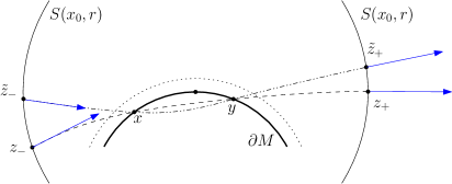
For every , both close to , consider the shortest geodesics and connecting them, in the metrics and , respectively. By the a priori estimate (2), those two geodesics lie in a neighborhood of of size which shrinks to zero, as and tends to zero, uniformly for all and satisfying (2). Next, we extend each one of them, lifted to the cotangent bundle (i.e., to the bicharacteristcs, called ”rays” below), in both directions until they hit . We denote by (respectively ), the common point with , and by (respectively ), the common point with , see Figure 3.
Let be the submanifold of consisting of all there such that the bicharacteristic through it, in the metric , is tangent to at some point close enough to . Let be the connected neighborhood of it consisting of those point staying at distance (with respect to fixed coordinates) at most with which we chose below. Then the small but -independent neighborhood of , admits the decomposition , where and are disconnected components, such that the rays form in the metric hit ; and the rays from do not. All of them are extended until they hit . We denote the corresponding travel times by , as in Section 2.2 but now is replaced by the geodesic sphere .
The rays issued from would hit and miss , by definition. They will stay at distance at least from . The same is true for the rays issued from related to the metric for , because by (44), the Hamiltonian vector fields of and are close, and . In particular, the rays related to will not hit for . Then
| (48) |
for over a compact interval. Recall that is the bicharacteristic issued from .
The rays issued from will hit at an angle at least , by the strict convexity. This is true, for , for the rays related to as well by the closeness of the Hamiltonians (outside ) argument. The travel times of the rays in the metric are in general different than but the points lie at distance to which decreases with in (2). Therefore, for , with would enter and leave it for , and it will also leave the neighborhood of where we modified . This is needed for the argument below.
| (49) |
Here, with uniquely determined as the contacts of the ray trough with . Also, by the closeness of the Hamiltonians outside , and by (47), the lengths of the segments of and from and , respectively, to their common point , differ by , see Figure 3. The segments in differ by , see (45). The remaining segments, after they exit and hit , differ by by the above argument. Therefore,
| (50) |
By (7),
| (51) |
We replace next by modulo errors controlled by (49), (50), so that we can get on the left; and use the fact that the latter satisfies (49). This would allow us to conclude that the integral is “small” in . Indeed, since is a smooth function with uniformly bounded derivatives for and bounded, we get by (49), (50),
| (52) |
This and (51) yield
| (53) |
where, in the last step, we used the second inequality in (49). The factor can be replaced by the square root of the distance between and the tangent manifold ; and that root is by construction. We choose so that to obtain ) in (53).
In , the even better estimate holds, without the term, by (48). In , we used the argument explained before to extend the estimate from to get an estimate there. By interpolation, we get
| (54) |
Now, by (7), (14), and (15) we can write the left-hand side of (54) in the form , and complete the proof of Theorem 5.1 by applying Proposition 3.3.
5.3. Global stability
For the purpose of the next theorem, we will extend and slightly generalize the foliation condition to compact submanifolds of . Let, as before, be a neighborhood of , and extend smoothly there. Note that the tilde over is not an indication that it is related to .
Definition 5.1.
Let be compact. We say that can be foliated by strictly convex hypersurfaces if there exists a smooth function which level sets , with some , restricted to , are strictly convex viewed from for ; is non-zero on these level sets, , and .
Note that this definition is not equivalent to Definition 1.1 when because in Definition 1.1, we allow to be non-empty (but with empty interior). Indeed, for uniqueness, proving outside such a set suffices since and are at least continuous. For stability however, it is convenient to assume that this set is empty.
We show next that the foliation condition implies non-trapping.
Proposition 5.1.
If can be foliated by strictly convex hypersurfaces, then any maximal geodesic in is of finite length.
Proof.
Assume that exists for and stays in ; and in particular, it never reaches for . The function cannot have more than one critical points as a consequence of the implication . By shifting the variable, we can always assume that the possible critical point is negative. Then is a strictly decreasing function for . On the other hand, it is bounded by below, so it has a limit , as , which is also its infimum. By compactness, there exists a sequence (we can start with and take a subsequence) so that converges to some . Next, . The limit must be tangent to at , because we can easily obtain a contradiction with the strict convexity if it is not. Now, by the strict convexity of again, there exists so that would hit for some positive time. This property is preserved under a small perturbation of ; and therefore applies to for . This contradicts the choice of however. ∎
In particular, we get the following.
Corollary 5.1.
Assume that , where can be foliated by strictly convex hypersurfaces, and is non-trapping. Then is non-trapping as well.
Note that can be a point, or a small neighborhood of a point, which happens if the level surfaces of are diffeomorphic to spheres but degenerates into a point. Another example is when is simple, see also the remarks following Theorem 1.3.
The norm below is defined in a fixed finite atlas of local coordinate charts. In the same way we define and its norm: in any coordinate system we can just take the supremum of and then the maximum over all charts. They can be defined in an invariant way, in principle but we do not do that for the sake of simplicity.
Theorem 5.2.
Assume that can be foliated by strictly convex hypersurfaces for . Let be a neighborhood of the compact set of all consisting of the initial points of all geodesics tangent to the intersections of the strictly convex hypersurfaces with . Then with , , , , , and as in Theorem 1.4, we have the stability estimate
| (55) |
for , satisfying (2).
Proof.
We will show first that the estimate in Theorem 1.4, near a boundary point , can be written in the form (55). For and on , both close to the fixed point , let be the boundary geodesic connecting (for ) and (for ). Set , where is the interior exponential map. Then ; set . Set
| (56) |
Then . On the other hand, in the notation following (1), given by ,
| (57) |
where is the tangential component of , the second component of . We also have
| (58) |
where is the second component of . Integrate the difference of (57) and (58) w.r.t. from to , and use (56) and the fact that on near to get (we get , actually). Note that this also proves that near . We remark that in the inductive step below, we will only have that and are close on near , instead of being equal. Then we would get instead of . So we get now as well. Since and are smooth and , we get
The constant in this estimate depends on the a priori bound in (2). We can therefore apply Theorem 5.1 to estimate the jet of at of any finite order. We then extend and in a neighborhood of so that and are there, as in (44).
For any geodesic in issued from , we extend it to and push the scattering relations and to . We show below that we have for the so extended lens relations, and a similar estimate for . We choose , and as the proof of Theorem 5.1 but this time is an neighborhood of (rather than , because the singualar factor is not present anymore). For any , let , be the points (in the phase space) of contact with the geodesic issued from for negative “times” with w.r.t. the metrics and , respectively. We define , in a similarly way, see Figure 4, where, in this case, , and . Then (the difference makes sense in local coordinates only) because we have the same for in . We have an bound of , and of the difference of the corresponding directions there, by the closeness of the scattering relations. Next, as well. Therefore, . Since and are smooth with uniformly bounded first derivatives, we also get , for all . We also have as shown in the paragraph following (58). In this step, we are no longer working near a fixed point on , and for almost tangential directions, the requirement for is that the geodesic issued from it are in the set required by the theorem but that set is a distance at least from the tangential set . In and , we argue as above.
Therefore, we have now that , where , and are defined as , and but with replaced by . We have the same for as well. The advantage of this is that the geodesics issued from hitting are never tangent to , and we actually have a uniform lower bound on the angle they make with . Thus we reduced the analysis to the case when is a priori known to be supported in the interior of .

We then apply a layer stripping argument finite number of times, see also the introduction in [49]. For each , assuming the estimate outside , we can choose an appropriate lens shaped domain near each point on , and artificial boundary close enough to it, see Figure 4. The closeness of and , and and implies the same for and by the arguments using (54). We do this for a finite number of points on by a compactness argument to prove the estimate in for some . We then cover with a finite set , and finish the proof with finitely many steps. ∎
6. Herglotz and Wieckert & Zoeppritz speeds are lens rigid
We revisit the Herglotz [14] and Wieckert and Zoeppritz [51] class of speeds. Let , be the ball in , centered at the origin with radius . The background metric in this section is the Euclidean one. Let be smooth in . Assume that satisfies the Herglotz and Wieckert & Zoeppritz condition
| (59) |
where is the radial derivative. We do not assume that is radial, i.e., that it depends on only. We show below that (59) is in fact a foliation condition.
Proposition 6.1.
The Herglotz and Wieckert & Zoeppritz condition (59) is equivalent to the the condition that the Euclidean spheres are strictly convex in the metric for .
Proof.
This proposition is essentially proved in [47, Proposition 7.1]. We will show first that the strict convexity condition of an oriented hypersurface (positive second fundamental form) is equivalent to the following: (A) if is the generator of the geodesic flow, and if is a defining function of positive on the “positive” side of , then when on a non-zero the energy level. In semigeodesic coordinates with on the “positive” side of , we have with on . Since
we have . On , ; therefore, (A) can be reformulated as follows: and imply . Differentiating again, we see that under those conditions, , where the Greek indices run from to . This is well known and follows directly form the definition to be the second fundamental form corresponding to the orientation . Then strict convexity, viewed from is equivalent to a negative second fundamental form. For manifolds with boundary we study, in the interior of , therefore convexity viewed from the exterior means a positive second fundamental form.
We can take as a defining function of the sphere for . Then . Next, and on the energy level , we have . Here and below, we still have summation w.r.t. even though both indices are upper. A direct computation shows that
with , therefore,
Therefore, on the unit energy level and for , strict convexity is equivalent to
i.e., , which is equivalent to (59). Note that the computations in [47, Proposition 7.1] are done in the cotangent bundle and are somewhat shorter. ∎
Note that we only require in Theorem 1.3 to satisfy (59). Then any other speed for which is still strictly convex and on with the same scattering relation is equal to . This extends the Herglotz [14] and the Wieckert & Zoeppritz [51] results to not necessarily radial speeds satisfying (59).
If (59) holds in the shell only, with some , then we get lens rigidity in the shell and we only need to use the scattering relation for geodesics staying in it. The speed does not even need to be defined in . We will skip the details.
References
- [1] G. Bao and H. Zhang. Sensitivity analysis of an inverse problem for the wave equation with caustics. J. Amer. Math. Soc., 27(4):953–981, 2014.
- [2] G. Besson, G. Courtois, and S. Gallot. Entropies et rigidités des espaces localement symétriques de courbure strictment négative. Geom. Funct. Anal., 5 (1995), 731–799.
- [3] D. Burago and S. Ivanov, Boundary rigidity and filling volume minimality of metrics close to a flat one. Ann. Math., 171 (2010), 1183–1211.
- [4] C. Croke. Scattering rigidity with trapped geodesics. Ergodic Theory Dynam. Systems, 34(3):826–836, 2014.
- [5] K. C. Creager. Anisotropy of the inner core from differential travel times of the phases PKP and PKIPK, Nature, 356(1992), 309–314.
- [6] C. B. Croke. Rigidity for surfaces of nonpositive curvature. Comment. Math. Helv., 65(1):150–169, 1990.
- [7] C. B. Croke. Rigidity and the distance between boundary points. J. Differential Geom., 33(2):445–464, 1991.
- [8] C. B. Croke. Rigidity theorems in Riemannian geometry. In Geometric methods in inverse problems and PDE control, volume 137 of IMA Vol. Math. Appl., pages 47–72. Springer, New York, 2004.
- [9] C. B. Croke and N. S. Dairbekov. Lengths and volumes in Riemannian manifolds. Duke Math. J., 125(1):1–14, 2004.
- [10] C. B. Croke and B. Kleiner. Conjugacy and rigidity for manifolds with a parallel vector field. J. Differential Geom., 39(3):659–680, 1994.
- [11] N. S. Dairbekov. Integral geometry problem for nontrapping manifolds. Inverse Problems, 22(2):431–445, 2006.
- [12] C. Guillarmou. Lens rigidity for manifolds with hyperbolic trapped set. arXiv:1412.1760, 2014.
- [13] M. Gromov. Filling Riemannian manifolds. J. Diff. Geometry 18 (1983), 1–148.
- [14] G. Herglotz. Über die Elastizitaet der Erde bei Beruecksichtigung ihrer variablen Dichte. Zeitschr. für Math. Phys., 52:275–299, 1905.
- [15] L. Hörmander. The analysis of linear partial differential operators, vol. 1-4. Springer-Verlag, 1983.
- [16] S. Ivanov. Volume comparison via boundary distances. Proceedings of the International Congress of Mathematicians, vol. II, 769–784, New Delhi, 2010.
- [17] V. Krishnan. A support theorem for the geodesic ray transform on functions. J. Fourier Anal. Appl. 15 (2009), 515–520.
- [18] V. Krishnan and P. Stefanov. A support theorem for the geodesic ray transform of symmetric tensor fields. Inverse Problems and Imaging, 3 (2009), 453–464.
- [19] M. Lassas, V. Sharafutdinov, and G. Uhlmann. Semiglobal boundary rigidity for Riemannian metrics. Math. Ann., 325(4):767–793, 2003.
- [20] R. B. Melrose. Spectral and scattering theory for the Laplacian on asymptotically Euclidian spaces. Spectral and scattering theory (Sanda, 1992). Lecture Notes in Pure and Appl. Math., 161, 85–130, Marcel Dekker, 1994.
- [21] R. Michel. Sur la rigidité imposée par la longueur des géodésiques. Invent. Math., 65(1):71–83, 1981/82.
- [22] R. G. Mukhometov. The reconstruction problem of a two-dimensional Riemannian metric, and integral geometry. Dokl. Akad. Nauk SSSR, 232(1):32–35, 1977.
- [23] R. G. Muhometov. On a problem of reconstructing Riemannian metrics. Sibirsk. Mat. Zh., 22(3):119–135, 237, 1981.
- [24] R. G. Muhometov and V. G. Romanov. On the problem of finding an isotropic Riemannian metric in an -dimensional space. Dokl. Akad. Nauk SSSR, 243(1):41–44, 1978.
- [25] C. Parenti, Operatori pseudo-differenziali in e applicazioni, Ann. Mat. Pura Appl. (4), 93 (1972), 359–389.
- [26] G. P. Paternain, M. Salo and G. Uhlmann. Tensor tomography on simple surfaces, Invent. Math., 193(2013), 229-247.
- [27] G. P. Paternain, M. Salo, G. Uhlmann. The attenuated ray transform for connections and Higgs fields, Geom. Funct. Anal. 22 (2012) 1460–1489.
- [28] G. P. Paternain, M. Salo and G. Uhlmann. Tensor tomography: progress and challenges, Chinese Annals of Math. Ser. B, 35(2014), 399–427.
- [29] L. Pestov and G. Uhlmann. Two dimensional compact simple Riemannian manifolds are boundary distance rigid. Ann. of Math. (2), 161(2):1093–1110, 2005.
- [30] L. N. Pestov and V. A. Sharafutdinov. Integral geometry of tensor fields on a manifold of negative curvature. Sibirsk. Mat. Zh., 29(3):114–130, 221, 1988.
- [31] A. Ranjan and H. Shah. Convexity of spheres in a manifold without conjugate points. Proc. Indian Acad. Sci. (Math. Sci.), 112 (2002), 595–599.
- [32] V. Sharafutdinov, M. Skokan, and G. Uhlmann. Regularity of ghosts in tensor tomography. J. Geom. Anal., 15(3):499–542, 2005.
- [33] V. A. Sharafutdinov. Integral geometry of tensor fields. Inverse and Ill-posed Problems Series. VSP, Utrecht, 1994.
- [34] V. A. Sharafutdinov. Integral geometry of a tensor field on a surface of revolution. Sibirsk. Mat. Zh., 38(3):697–714, iv, 1997.
- [35] V. A. Sharafutdinov. A problem in integral geometry in a nonconvex domain. Sibirsk. Mat. Zh., 43(6):1430–1442, 2002.
- [36] V. A. Sharafutdinov, Variations of Dirichlet-to-Neumann map and deformation boundary rigidity of simple 2-manifolds. J. Geom. Anal. 17 (2007), 147–187.
- [37] M. A. Shubin, Pseudodifferential operators in , Dokl. Akad. Nauk SSSR, 196 (1971), 316–319.
- [38] P. Stefanov. Microlocal approach to tensor tomography and boundary and lens rigidity. Serdica Math. J., 34(1):67–112, 2008.
- [39] P. Stefanov and G. Uhlmann. Rigidity for metrics with the same lengths of geodesics. Math. Res. Lett., 5(1-2):83–96, 1998.
- [40] P. Stefanov and G. Uhlmann. Stability estimates for the X-ray transform of tensor fields and boundary rigidity. Duke Math. J., 123(3):445–467, 2004.
- [41] P. Stefanov and G. Uhlmann. Boundary rigidity and stability for generic simple metrics. J. Amer. Math. Soc., 18(4):975–1003, 2005.
- [42] P. Stefanov and G. Uhlmann. Boundary and lens rigidity, tensor tomography and analytic microlocal analysis. In Algebraic Analysis of Differential Equations. Springer, 2008.
- [43] P. Stefanov and G. Uhlmann. Integral geometry of tensor fields on a class of non-simple Riemannian manifolds. Amer. J. Math., 130(1):239–268, 2008.
- [44] P. Stefanov and G. Uhlmann. Local lens rigidity with incomplete data for a class of non-simple Riemannian manifolds. J. Differential Geom., 82(2):383–409, 2009.
- [45] P. Stefanov and G. Uhlmann. Recovery of a source term or a speed with one measurement and applications, Trans. Amer. Math. Soc., 365, 5737–5758, 2013.
- [46] P. Stefanov and G. Uhlmann. The geodesic X-ray transform with fold caustics. Anal. PDE, 5, 219–260, 2012.
- [47] P. Stefanov and G. Uhlmann. Multi-wave methods via ultrasound. In Inside Out, volume 60, pages 271–324. MSRI Publications, 2012.
- [48] H. Triebel. Interpolation theory, function spaces, differential operators, volume 18 of North-Holland Mathematical Library. North-Holland Publishing Co., Amsterdam, 1978.
- [49] G. Uhlmann and A. Vasy. The inverse problem for the local geodesic ray transform. preprint, arXiv:1210.2084.
- [50] J. Vargo. A proof of lens rigidity in the category of analytic metrics, Math. Research Letters, 16 (2009), 1057–1069.
- [51] E. Wiechert and K. Zoeppritz. Über Erdbebenwellen. Nachr. Koenigl. Geselschaft Wiss. Göttingen, 4:415–549, 1907.
- [52] H. Zhou. The inverse problem for the local ray transform. Preprint. arXiv:1304.7023, 2013.