Estimating the uncertainty in underresolved nonlinear dynamics

Abstract

The Mori-Zwanzig formalism of statistical mechanics is used to estimate the uncertainty caused by underresolution in the solution of a nonlinear dynamical system. A general approach is outlined and applied to a simple example. The noise term that describes the uncertainty turns out to be neither Markovian nor Gaussian. It is argued that this is the general situation.

1 Introduction

There are many problems in science where it is impractical to find fully resolved numerical solutions of the problems of interest, and one needs to estimate the resulting uncertainty. For example, there are situations, e.g. in geophysics and in economics, where one wants to estimate the state of a system on the basis of noisy underresolved equations supplemented by a stream of noisy data (see e.g. [7, 4]); this is the “filtering” or “data assimilation” problem, which requires that a probability density of the noise be provided. There are similar problems in turbulence calculations, where one wants to model the impact of the motion at one set of scales on the motion at another scale (see e.g [1, 15]), i.e. one wants to estimate the difference between a full system and one in which a given set of components is absent. In such settings, one often makes the assumption that the missing information can be represented as white noise, though it is well understood that this is justifiable only where the scales are separated, i.e., when the components that are not computed are faster and smaller than the ones that one is solving for (see e.g. [19]), and that separation of scales fails to hold in many problems of interest. Here we present a construction that does not rely on separation of scale, and use it to illustrate the intrinsic features of the problem.

It is important to note that what one needs is an estimate of the uncertainty in the equations, not in the results. For example, in data assimilation, it is the uncertainty in the equations that is combined with the uncertainty in the data to produce an estimate of the overall uncertainty in the state. Consider for example a system of ordinary differential equations of the form

$$\frac{d}{dt}\phi=R(\phi),$$ (1)

with initial data $\phi(0)=x$. Assume that $\phi$ has components $\phi_{1},\phi_{2},\dots,\phi_{K}$, only the first $k<K$ of which can be effectively computed. Define ${\hat{\phi}}=(\phi_{1},\dots,\phi_{k})$ and ${\tilde{\phi}}=(\phi_{k+1},\dots,\phi_{K})$. Similarly, partition the right-hand side of the equation as $R=(\hat{R},\tilde{R})$ and the data as $x=(\hat{x},\tilde{x})$. The underesolved equations that we are able to solve have the form

$$\frac{d}{dt}\psi=\mathcal{R}(\psi),$$ (2)

where $\psi$ is an approximation of $\hat{\phi}$, $\mathcal{R}$ is an approximation of $\hat{R}$, and $\psi(0)=\hat{x}$ (when one underresolves, one approximates functions of many variables by functions of fewer variables, as when one uses $k$ Fourier components to approximate a differential operator when $K>k$ are needed). The estimate of the uncertainty is a function $n(t)$, the “noise”, which, added to $\mathcal{R}$, would make the solution of equation (2) approximate the first $k$ components of the solution of equation (1); i.e., we are hoping that approximately, in a sense to be determined, one would have:

$$\frac{d}{dt}\hat{\phi}=\mathcal{R}(\hat{\phi})+n(t),$$ (3)

with initial data $\phi(0)=\hat{x}$. The term $n(t)$ would be the estimate of the uncertainty in the underresolved system (2). Equation (3) obviously holds if one sets

$$n(t)=\hat{R}(\phi)-\mathcal{R}(\hat{\phi}).$$ (4)

So that, if one can find $\phi$, one can estimate $n(t)$. But if one has $\phi$, there is no need to find $\psi$ or $n$.

The problem becomes more interesting if it is randomized as in [10, 25] and in the Mori-Zwanzig theory (see e.g. [8, 9, 26, 3, 6]). Equations (1) and equations (2) need initial data of different dimension; to compare their solutions one has to decide what to do with the extra components $\tilde{x}$ of the initial vector $x$. In practical problems $\tilde{x}$ is unknown, and we assume that it is sampled from some suitable known probability density, maybe deduced from previous knowledge, for example, if the problem comes from weather forecasting, ample records of previous weathers can be put to use. The function $\phi(t)$ becomes a stochastic process $\phi(t)=\phi(t,\omega)$ where $\omega$ is an element of a probability space, and similarly $n=n(t,\omega)$. The advantages of this probabilistic setting are: (i) in practical problems one is typically interested in a range of possible missing data, rather than in some specific missing datum; (ii) in data assimilation problems a probabilistic formulations is essential; and, most important, (iii) it is often possible to say something general and useful about the probability density of missing data when one cannot say anything useful about any particular missing datum (an example will be given in the present paper). A further discussion of the merits of this formulation will be given in the concluding section of this paper.

In the present paper we assume in addition that enough information about the the statistics of $\phi$ is available (for specifics, see section 4). Of course one wishes to eventually solve problems where this information is not available, but looking at what happens when it is available is already instructive. We disregard here all sources of uncertainty other than underresolution, except for a comment in the conclusions section, though they too can be handled by the our formalism.

It is of course desirable to make $n(t)$ as small as possible. In the present paper a low noise intensity is reached by using the Mori-Zwanzig formalism of statistical mechanics [8, 9, 26, 3, 6], which draws as much information as possible into the resolved part of the calculation.

In the next section we summarize the Mori-Zwanzig formalism in the version we need. In section 3 we present our example. In section 4 we present numerical results. Conclusions are drawn at the end of the paper.

There is a large literature on noise modeling. A general theoretical overview can be found in [21]. Related numerical work is summarized in [11]. Powerful techniques aimed at geophysical problems can be found in [16, 13]. A particularly interesting approach, for situations where the problem can be approximately viewed as linear, can be found in [17]. The work in the present paper has a kinship with the stochastic parametrization proposal of Wilks [22], see also [12], though the mathematical and statistical tools differ, and we are estimating the noise rather than parametrizing, i.e., estimating the variance rather than trying to improve the calculation of the mean. The technical difficulties discussed below make us doubt that the latter goal is achievable, but if it is, the Mori-Zwanzig formalism could be useful there as well.

The use of the Mori-Zwanzig formalism for estimating uncertainty was pioneered in [20] where a much more sophisticated implementation was used to quantify the uncertainty due to uncertain parameters in a differential equation, without assuming that the full solution of the problem was already available. However, the simpler analysis in the present paper lends iself well to the particular purpose here, which to demonstrate the persistence of memory in underresolved dynamics.

2 The Mori-Zwanzig (MZ) formalism

We largely follow here the exposition in [3] with suitable modifications ; see also [2]. Note that our main tool, equation (11) below, can be derived without the full MZ formalism, as indicated there; we provide the more general formalism because it is needed for some comparisons later.

Consider again the system (1) above,

$$\frac{d}{dt}\phi=R(\phi(t)),\;\;\phi(x,0)=x.\;\;$$ (5)

Denote the solution of this equation by $\phi(x,t)$, making its dependence on the initial conditions explicit. Partition the vector $\phi$ as above into resolved variables $\hat{\phi}$ and unresolved variables $\tilde{\phi}$, and similarly set $x=(\hat{x},\tilde{x})$ and $R=(\hat{R},\tilde{R})$. Form the Liouville partial differential equation

$$u_{t}=Lu,$$ (6)

where $u=u(x,t)$ satisfies the initial condition $u(x,0)=g(x)$, $g$ is a given function and

$$L=\sum R_{j}(x)\frac{\partial}{\partial x_{j}}.$$ (7)

One can show that the solution of this equation is $u(x,t)=g(\phi(x,t))$, where $\phi(x,t)$ is the solution of equations (1). In particular, if $g(x)=x_{j}$, it follows that $u(x,t)=\phi_{j}(x,t)$, where $x_{j},\phi_{j}$ are the $j-$th components of respectively $x$ and $\phi$. Denote the solution of the Liouville equation with datum $g(x)$ by $u=e^{tL}g(x)$ (this is the “semigroup notation”). In this notation, the identity $u(x,t)=g(\phi(x,t))$ becomes

$$e^{tL}g(x)=g(e^{tL}x).$$ (8)

This identity shows that that the Liouville equation, which is linear, is equivalent to the (generally nonlinear) system of ordinary differential equations (1); the solution of equations (1) provides the solution of the Liouville equation, and conversely, if the Liouville equation can be solved for any initial function $g(x)$, one obtains the $i-th$ component $\phi_{i}$ of (1) by solving the Liouville equation with $g(x)=x_{i}$. One can also prove the identity:

$$e^{tL}L=Le^{tL}.$$ (9)

At time $t=0$ assign to the initial data $\hat{x}$ specific fixed values, and sample the initial data $\tilde{x}$ from a suitable probability density, as described in the introduction. The conditional expectation $E[h(x)|\hat{x}]$ of a function $h$ of $x$ given $\hat{x}$ is well-defined, and is an orthogonal projection of $h$ on the space of functions of $\hat{x}$. Define the conditional expectation operator at the initial time $P$ by $Ph=E[h|\hat{x}]$ for any function $h$, and define and $Q=I-P$, where $I$ is the identity operator. Clearly $P,\,Q$ are both orthogonal projections and $P+Q=I$.

Pick as an initial datum for the Liouville equation the vector $\hat{x}$, i.e., consider only the first $k$ equations in equation (1). Using the notation $u=e^{tL}\hat{x}$, the Liouville equation becomes:

$$\frac{\partial}{\partial t}e^{tL}\hat{x}=Le^{tL}\hat{x}=e^{tL}L\hat{x}=e^{tL}(P+Q)L\hat{x},$$ (10)

where the commutation relation (9) has been used. One can readily check that $Lx_{j}=R_{j}$, so that

$$PL\hat{x}=E[\hat{R}|\hat{x}],$$

which is a function of $\hat{x}$ only; call this function $\bar{R}=\bar{R}(\hat{x})$. It follows that $e^{tL}QL\hat{x}=\hat{R}(\phi)-\bar{R}(\hat{\phi})$. Equation (10) is equivalent to the equation

$$\frac{d}{dt}\hat{\phi}=\bar{R}(\hat{\phi})+\left(\hat{R}(\phi)-\bar{R}(\hat{\phi})\right).$$ (11)

We propose to set $\mathcal{R}=\bar{R}$ in equation(2) which defines the underresolved approximation, so that

$$\frac{d}{dt}\psi=\bar{R}(\psi).$$ (12)

The noise, as defined in equation (4), is $n(t)=\hat{R}(\phi)-\bar{R}(\hat{\phi})$. Equation (11) is the main tool used in this paper; note that one can get to it by simply setting $\mathcal{R}=\bar{R}$ in equation (3); the full MZ development is presented because it is needed in the discussion.

The derivation of the Mori-Zwanzig generalized Langevin equation requires several more steps. Any two linear operators $A$ and $B$ satisfy the following identity (the Dyson or Duhamel formula):

$$e^{t(A+B)}=e^{tA}+\int_{0}^{t}e^{(t-s)(A+B)}Be^{sA}\,ds.$$ (13)

Substituting $A=QL$ and $B=PL$, this becomes:

$$e^{tL}=e^{tQL}+\int_{0}^{t}e^{(t-s)L}PLe^{sQL}\,ds.$$ (14)

Substituting into (11), one finds:

$$\frac{\partial}{\partial{t}}e^{tL}\hat{x}=e^{tL}PL\hat{x}+e^{tQL}QL\hat{x}+\int_{0}^{t}e^{(t-s)L}PLe^{sQL}QL\hat{x}\,ds,$$ (15)

where $e^{tL}\hat{x}=\hat{\phi}$. This is the Mori-Zwanzig (MZ) generalized Langevin equation. The evaluation of the last two terms is in general difficult; an algorithm was proposed in [2] but it is too laborious for practical use. Equation (15) is in general not Markovian, and the memory term is in general non-zero, so that one cannot expect the noise $n(t)$ in equation (11) to have zero mean.

The MZ equation can be simplified by approximating the operator $e^{tQL}$ in the integrand of the third term by $e^{tL}$ (see [2, 3]). With this approximation, the integral term simplifies to:

$$\int_{0}^{t}e^{tL}PLQL\hat{x}ds=te^{tL}LQL\hat{x}.$$

The memory term has been reduced to a differential operator multiplied by the time $t$; the time starts at $t=0$ when the initial values are assigned and when there is no uncertainty in the resolved variables.

If one is interested only in the conditional expectations of $\hat{\phi}(t)$, one can premultiply equation by the conditional averaging operator $P$; the noise term then drops out, so that the MZ equation with the simplified integral term becomes

$$\frac{\partial}{\partial t}P\phi(t)=Pe^{tL}PL\hat{x}+tPe^{tL}PLQL\hat{x}.$$ (16)

In the absence of the noise term the conditional expectation of a nonlinear function of $\phi$ cannot be ascertained without approximation; we resort here to “mean field” closure $PH(\phi)=H(P\phi)$ for any function $H=H(\phi)$, in particular for the functions $G(\phi)=PLQL(\hat{\phi})$ and $F(\phi)=PL(\hat{\phi})$, so that

$$\frac{\partial}{\partial t}\Phi=F(\Phi)+tG(\Phi),$$ (17)

where $\Phi=P\phi$. This is the $t$-model approximation of the MZ equations (see [2, 3]).

3 A model problem

The dynamical system to which the theory of the preceding section will be applied is now presented. It is a Hamiltonian system with $m+1$ particles, one of which is resolved, or “tagged”, and the others are unresolved. The Hamiltonian is

$$H=(1/2)(p^{2}+q^{2}+\sum_{1}^{m}p_{i}^{2}/g_{i}+(\sum_{1}^{m}q_{i}^{2})/\epsilon+\alpha q^{2}\sum_{1}^{m}q_{i}^{2}),$$ (18)

where $q,p$ are the position and the momentum of the tagged particle, $q_{i},p_{i}$ are the positions and momenta of the $m$ other particles, $\alpha,\epsilon,$ and $g_{i},i=1,\dots,m$ are parameters; $\epsilon$ quantifies the amount by which the unresolved particles are faster that the tagged particle; $\alpha$ quantifies the strength of the interaction between the tagged and unresolved particles, the parameters $g_{i}$ control the periods of the unresolved particles; in the examples below, $\alpha=\epsilon=m^{-1}$ and $g_{1}=\sqrt{5}/2,\,g_{2}=\sqrt{3}/2.$ Except when stated otherwise, $m=2.$ The underresolved system is one in which only the tagged particle is solved for, so that in the notations of the introduction, $k=2$ and $K=2m+2$. Note that the notation for the variables has changed from $\phi$ to $q,p$, the latter being more transparent for a Hamiltonian system. This system of equations is a generalization of the example used in [2, 3] to demonstrate the properties of the MZ formalism; it resembles the model problems studied in [10, 25] but is more strongly nonlinear. This system is not ergodic; to demonstrate this, figure 1 shows the projection of a single trajectory of the system on the $(q,p)$ plane; if the system were ergodic, there would be no hole in the donut.

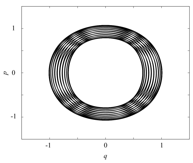
Figure 1: Ergodicity check.

A non-ergodic system is studied because of the expectation that the constructions below will be used in problems with persistent states, as in weather forecasting (see e.g. [24]).

A time $t=0$ one specifies initial values for $q(0),p(0)$ for the tagged variable, and one samples the $q_{i},p_{i}$ from the canonical density $e^{-H/T}/Z$ conditioned by $q(0),p(0)$; here $T$ is a “temperature” (which will be set equal to $1$ for simplicity) and $Z$ is the partition function. The equations of motion are:

$$\frac{d}{dt}q= p,$$

$$\frac{d}{dt}p= -q(1+\alpha\sum_{1}^{m}q_{i}^{2}),$$

$$\frac{d}{dt}q_{i}= p_{i}/g_{i},\,\,\,\,\,\,i=1,\dots,m,$$

$$\frac{d}{dt}p_{i}= -q_{i}(1+\epsilon\alpha q^{2})/\epsilon,\,\,\,\,\,\,i=1,\dots,m.$$ (19)

The Liouville operator $L$ is:

$$L=p\frac{\partial}{\partial q}-q(1+\alpha\sum_{1}^{m}q_{i}^{2})\frac{\partial}{\partial p}+\sum(p_{i}/g_{i})\frac{\partial}{\partial q_{i}}-\sum_{1}^{m}(q_{i}(1+\epsilon\alpha q^{2})/\epsilon)\frac{\partial}{\partial p_{i}}.$$ (20)

Elementary calculations yield:

$$E[q(1+\alpha\sum_{1}^{m}q_{i}^{2}|q,p]=q\left(1+\frac{m\alpha\epsilon}{1+\alpha\epsilon q^{2}}\right),$$ (21)

while of course $E[p|q,p]=p$. The equations $\frac{d}{dt}\hat{\phi}=E[\hat{R}|\hat{\phi}]$ reduce to a two-component Hamiltonian system with Hamiltonian

$$\hat{H}=(1/2)(p^{2}+q^{2}+m\log(1+\alpha\epsilon q^{2})).$$

Similarly, the vector $\hat{R}(\phi)-E[R(\phi)|\hat{\phi}]$ has components $(0,n(t))$ where

$$n(t)=-q\left(\frac{m\alpha\epsilon}{1+\alpha\epsilon q^{2}}-\alpha\sum_{1}^{m}q_{i}^{2}\right).$$ (22)

In doing these calculations, it was assumed that:

$$E[f(q,q_{i},p,p_{i})|q,p]=\frac{\int f(q,q_{i},p,p_{i})e^{-H}\,dq_{i}\,dp_{i}}{\int e^{-H}\,dq_{i}\,dp_{i}}$$

for an arbitrary function $f$, where $q_{i}$ stands for $q_{1},q_{2},\dots,q_{m}$, similarly for $p_{i}$; $dq_{i}$ stands for $dq_{1}\cdots dq_{m}$, and similarly for $dp_{i}$; the Hamiltonian $H$ is a function of all the variables. The integrations are over the whole hyperplane where $q$ and $p$ are constant; the non-ergodicity of the system is not taken into account.

Suppose one wants to calculate the conditional expectation of the resolved variables $q,p$ given their initial values $q(0),p(0)$. In the low-dimensional example here this calculation can be done from first principles. Given $q,p$ at time $t=0$, one can repeatedly sample the coordinates and momenta of the unresolved particles from the initial probability density $e^{-H}/Z$; for each set of initial data, one can solve the full system of equations up to a time $t$; one can then average the values of $q(t),p(t)$ in these solutions; the result is, by definition, the conditional expectations $E[q(t)|q(0),p(0)],E[p(t)|q(0),p(0)]$.

On the other hand, one can derive and solve the MZ equations in the $t-$model approximation. Elementary calculations show that these equations reduce to:

$$\frac{d}{dt}Q= P,$$ (23)

$$\frac{d}{dt}P= -Q(1+\frac{m\alpha\epsilon}{1+\alpha\epsilon Q^{2}})-\frac{2m\alpha^{2}\epsilon^{2}Q^{2}Pt}{(1+\alpha\epsilon Q^{2})^{2}},$$ (24)

where $Q=E[q(t)|q(0),p(0)],P=E[p(t)|q(0),p(0)].$ (For a related example where the intermediate steps in the derivations are presented in detail, see [3]).

In figure 2 the values of $Q=E[q(t)|q(0),p(0)]$ computed from first principles, with no approximations other than use of the law of large numbers, are compared with the results of $t$-model, with $m=2$.

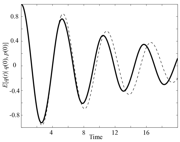
Figure 2: Time decay of conditional expectations: $t$-model (thick line) vs. the truth (thin dashed line).

It should be obvious that the MZ formalism would give less noisy solutions when $m$, the number of unresolved particles, increases, because then the instantaneous average of their effects on the tagged particle approaches its average with respect to the invariant measure, making the problem less interesting. We list again the approximations used in deriving the $t-$model results: (i) the substitution $e^{tQL}=e^{tL}$ in the memory term; (ii) the mean field approximation; (iii) no account taken of the nonergodicity of the dynamics; in addition, (iv), the measure with density $e^{-H}/Z$ is invariant at equilibrium, but since at $t=0$ the location and momentum $q,p$ of the tagged particle are fixed, the system is not in equilibrium. One cannot expect the agreement in figure 2 to be perfect.

The conditional expectations decay in time because, in the presence of noise, the predictive value of initial data decays in time. The uncertainty in the unresolved data affects the resolved variables, each random solution goes its own way, and while each preserves the Hamiltonian, the average of the solutions converges to the equilibrium average, which here is zero. The decay in the expected value is due entirely to the uncertainty.

4 Numerical analysis of the noise

The program outlined in section 2 will now be implemented in the special case described in the preceding section. The first step is the analysis of the noise term $n(t)$ described in equation (22). We have assumed that the noise is known in principle– if the solutions of the full system are known, formula (22) above represents the noise. To be useful, for example in data assimilation, one needs an explicit representation of the noise in terms of a small number of parameters, and the goal in the present section is to derive such a representation approximately.

The function $q(t)$ is resolved and therefore available at every step, so the function one has to represent is:

$$z(t)=n(t)/q(t)=-\frac{m\alpha\epsilon}{1+\alpha\epsilon q^{2}}+\alpha\sum_{1}^{m}q_{i}^{2},$$ (25)

The system (1) is stationary with an invariant canonical probability density $e^{-H}/Z$. Initial data (including data for the tagged variable) were sampled from this invariant density repeatedly; for each initial vector, the differential equations (19) were solved numerically, the function $z(t)$ was evaluated, and the covariance function $C(\tau)=E[z(0)z(\tau)]$ was computed. We observed that as $\tau\rightarrow\infty$, $C(\tau)$ converged to a constant $A$. We exhibit this convergence in table 1, where we list values of $C(\tau)$ for various values of $\tau$, as well as values of the integrated covariance $C^{*}(\tau)=\tau^{-1}\int_{0}^{\tau}C(s)ds$ which, in this oscillatory system, converge to their limit faster than $C(\tau)$ as $\tau$ increases.

Table 1: Convergence of $C(\tau)$ to a limit

$\tau$	$C(\tau)$	$C^{*}(\tau)$
0	0.1967	0.1967
1	0.0046	0.1018
2	0.1771	0.0961
3	0.0289	0.0999
4	0.1398	0.0943
5	0.0621	0.0971
6	0.1072	0.0940
7	0.0863	0.0949
8	0.0909	0.0941
9	0.0927	0.0935
10	0.0922	0.0941
11	0.0860	0.0928
12	0.1009	0.0937
13	0.0783	0.0926
14	0.1054	0.0932
15	0.0765	0.0926
16	0.1062	0.0928
17	0.0787	0.0926
18	0.1041	0.0926
19	0.0828	0.0927

We then decomposed $C(\tau)$ in the form:

$$C(\tau)=\beta(\tau)+A,$$ (26)

where $\beta(\tau)$ tends to zero as $\tau$ increases.

Table 2: Computed covariances

$\tau$	$C(\tau)$	$\beta(\tau)$
0.00	0.1967	0.1008
0.05	0.1953	0.0994
0.10	0.1917	0.0958
0.15	0.1860	0.0901
0.20	0.1782	0.0823
0.25	0.1686	0.0727
0.30	0.1574	0.0615
0.35	0.1449	0.0490
0.40	0.1313	0.0354
0.45	0.1170	0.0212
0.50	0.1024	0.0065

Furthermore, for each set of initial data, the quantity $\tau^{-1}\int_{0}^{\tau}z(0)z(s)ds$, whose expected value is $C(\tau)$, individually converged to a limit, say $a$, which is a function of the random initial values, so that $a=a(\omega)$, with

$$A=E[a],$$ (27)

where $A$ is the constant in equation (26). The parameter $a$ is a “persistence parameter”, embodying the fact that in a non-ergodic system the initial values are never fully forgotten. It was pointed out in section 2 that one cannot expect $n(t)$ to have a zero mean. The variable $a$ is roughly log-normal; in figure 3 we display a histogram of $\log a$.

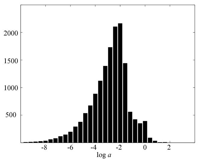
Figure 3: Histogram of $\log a$.

The calculations that produced these figures were performed with a fourth-order Runge-Kutta method with time step $k=0.05$, repeated 20000 times to get the statistics.

The stochastic process $n(t)$ was modelled as the sum of a stationary time series $b(t,\omega)$, with a discrete step $k$ and with a covariance that approximates $\beta(\tau)$, to which, at each step, was added the square root of a sample of the persistence parameter $a$, sampled at time $t=0$ and left constant during each time evolution; this satisfies equation (26). The covariance of the time series was approximated by a covariance of the form $C(\ell k)=\beta_{0}\,d^{|\ell|}$, where $\ell$ is an integer, the coefficient $\beta_{0}$ is read from table 2, and the parameter $d$ is obtained by a least-squares fit of $C(\ell k)$ to the the computed function $\beta(\tau)$ in the interval $[0,\tau_{0}]$, where $\tau_{0}$ is the first zero of $\beta(\tau)$. In the case where $k=0.05$ and $n=2$, this gave the value $d=.902$; if one changes the numerical time step from $k=0.05$ to $k=k^{*}$, $d$ becomes $d^{*}=d^{(k^{*}/0.05)}$. With this representation of $C(\ell k)$, the time series $b(\ell k)$ becomes a two-step recursion, so that if $b(jk)$ has been sampled at time $jk$ and its value was $B(jk)$, then at time $(j+1)k$ the sample value is $B((j+1)k)=d\cdot B(jk)+\xi$, where $\xi$ is sampled from an independent Gaussian distribution with mean zero and variance $\beta_{0}(1-d^{2})$ (see e.g. [23, 3]). The values of $a$, one per sample of the initial data, were sampled using the histogram above.

The modeled stochastic process is the estimate of the uncertainty in the underresolved system we propose to use when an explicit representation of the noise is needed, for example in data assimilation. Note that an equilibrium distribution of $n(t)$ is used though the system (19) is solved with some of the data having fixed values, i.e., it is not in equilibrium. This parallels the approximations made in the application of the MZ formalism in section 2.

As a check on the validity of this representation, consider the solution of the system (3) with $n(t)$ sampled with the help of this representation. The system $\frac{d}{dt}\psi=\bar{R}(\psi)$ is Hamiltonian, so that the decay of the solutions of

$$\frac{d}{dt}\psi=\bar{R}(\psi)+n(t),$$ (28)

which should match the true decay, is due entirely to the presence of the noise $n(t)=p(t)z(t)$. In figure 4 we compare the average of the solutions of equation (28), with fixed initial values but random forcing $n(t)$, to the exact average computed in section 3.

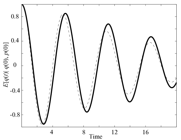
Figure 4: Time decay of conditional expectations: the noise model (thick line) vs. the truth (thin dashed line).

In figure 5 we compare the histogram of the values of $q(t)$ at time $t=20$ (a long time) obtained by solving repeatedly the full system (19), with the histogram obtained by solving the reduced system (28) where the noise is sampled from the representation above.

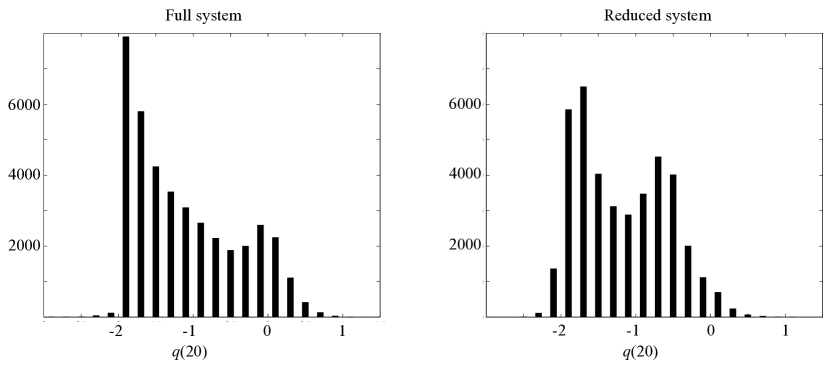
Figure 5: Histograms of q(t) at time t=20: the noise model vs. the truth.

The random equations (28) were solved by the Klauder-Petersen scheme [14]; a rationale for this choice can be found in [18]. The time step was $k=0.01$. Note that equations (28) can be interpreted as a numerical implementation of the full MZ Langevin equation (15).

These comparisons validate the representation of the noise; indeed, the conditional expectations here are significantly closer to the truth than the one obtained with the $t$-model approximation.

5 Conclusions

In subsequent publications we expect to demonstrate the use of the formalism presented in this paper in more interesting cases. We think that the features of the noise seen in the particular case discussed above– the fact that it is non-Gaussian and non-Markovian – are general, and that the practice of data assimilation should take this into account.

The non-Gaussianity is not surprising. The equations solved are non-linear and their invariant measure is non-Gaussian, and there can be no expectation that the uncertainty in their solution is Gaussian. The strongly non-Markovian nature of the noise is more interesting. It has been built into the model by the assumption that the only randomness is in the the initial data, while the time evolution is deterministic. This is the right assumption for the assessment of the uncertainty due to underresolution in differential equations. The fully resolved true solution of the problem satisfies a differential equation, one whose solution one may be unable to find, but a differential equation none-the-less. The underresolved system one can solve approximates a differential equation. The difference between solutions of differential equations cannot be memoryless. These comments remain valid if the equations are chaotic- the size of the uncertainty may grow, but chaotic dynamics described by differential equations are not memoryless either. The same is true if one chooses to model unresolved inputs as stochastic processes; they may modify the memory but not annihilate it.

The present paper complements the work in [5], where it was shown that in physically reasonable vector-valued data assimilation problems, the various one-time components of the noise must be correlated; in particular, they must be spatially correlated if the several components describe physical variables estimated at different spatial points. In the present paper we show that the noise components must be are correlated in time as well.

6 Acknowledgements

We would like to thank Prof. R. Miller, of Oregon State University, for advice, references, and illuminating discussions about error modelling in geophysical fluid dynamics, and our colleague Dr. Matthias Morzfeld for help with in the preparation of this paper. This work was supported in part by the Director, Office of Science, Computational and Technology Research, U.S. Department of Energy under Contract No. DE-AC02-05CH11231, and by the National Science Foundation under grant DMS-1217065.

References

- [1] A. Bensoussan, Stochastic Navier-Stokes equations, Acta. Appl. Math. 38 (1995), pp. 267-304.
- [2] A. J. Chorin, O.H. Hald, and R. Kupferman, Optimal prediction with memory. Physica D 166 (2002), pp. 239-257.
- [3] A.J. Chorin and O.H. Hald, Stochastic Tools for Mathematics and Science. Springer- Verlag, New York, 2013.
- [4] A.J. Chorin and X. Tu, Implicit sampling for particle filters, Proc. Nat. Acad. Sc. USA 106 (2009), pp. 17249-17254.
- [5] A.J. Chorin and M. Morzfeld, Conditions for successful data assimilation, under review, J. Geophys. Res. 2013.
- [6] A.J. Darve, J. Salomon, and A. Kia, Computing generalized Langevin equations and generalized Fokker-Planck equations, Proc. Nat. Acad. Sc. USA 27 (2009), pp. 10884-10889.
- [7] A. Doucet, N. de Freitas, and N. Gordon, Sequential Monte Carlo Methods in Practice, Springer, NY, 2001.
- [8] D. Evans and G. Morriss, Statistical Mechanics of Nonequilibrium Liquids, Academic Press, London, 1990.
- [9] E. Fick and G. Sauerman, The Quantum Statistics of Dynamical Processes, Springer, 1990.
- [10] G. Ford, M. Kac, and P. Mazur, Statistical mechanics of assemblies of coupled oscillators, J. Math. Phys. 6 (1965), pp. 504-515.
- [11] R. Ghanem and P. Spanos, Stochastic Finite Elements: A Spectral Approach, Springer, New York, 1991.
- [12] T. Hamill and J. Whitaker, Accounting for the error due to unresolved scales in ensemble data assimilation: a comparison of different approaches, Month. Weather Rev. 133 (2005), pp. 3132-3247.
- [13] E. Kalnay, Atmospheric Modeling, Data Assimilation and Predictability, Cambridge, 2003.
- [14] J. Klauder and W. Petersen, Numerical integration of multiplicative-noise stochastic differential equations, SIAM J. Num. Anal. 22 (1985), pp. 1153-1166.
- [15] S. Kuksin and A. Shirikyan, Mathematics of Two-Dimensional Turbulence, Cambridge, 2012.
- [16] A. Majda and J. Harlim, Filtering Complex Turbulent Systems, Cambridge, 2012.
- [17] J. Richman, R. Miller, Y. Spitz, Error estimates for assimilation of satellite sea surface temperature data in ocean climate models, Geophys. Res. Lett. 32 (2005), DOI:10.1029/2005GL023591.
- [18] M. Morzfeld, X. Tu, E. Atkins, and A.J. Chorin, A random map implementation of implicit filters, J. Comp. Phys. 231 (2012),pp. 2049-2066.
- [19] G. Papanicolaou, Introduction to the asymptotic analysis of stochastic equations, in “Modern Modeling of Continuum Phenomena”, R. DiPrima (ed.), Providence RI, 1974.
- [20] Mori-Zwanzig reduced models for uncertainty quantification I: parametric uncertainty, arXiv:1211.4285v1 [math.NA] 19Nov2012.
- [21] A.M. Stuart. Inverse problems: a Bayesian perspective, Acta Numerica (19), 2010. pp 451-559
- [22] D. Wilks, Effects of stochastic parametrization in the Lorenz ’96 system, Quart. J. Roy. Meteo. Soc. 131 (2005), pp. 389-407.
- [23] A. Yaglom, An Introduction to the Theory of Stationary Random Functions, Dover, New York, 1962.
- [24] X. Yang, W. Ren, and E. Vanden Eijnden, Nonequilibrium statistical mechanics of climate variability, submitted for publication, 2013.
- [25] R. Zwanzig, Nonlinear generalized Langevin equations, J. Stat. Phys., 9, (1973), pp. 215-220.
- [26] R. Zwanzig, Nonequilibrium Statistical Mechanics, Oxford, 2001.