Graphs with Plane Outside-Obstacle Representations

Abstract

An obstacle representation of a graph consists of a set of polygonal obstacles and a distinct point for each vertex such that two points see each other if and only if the corresponding vertices are adjacent. Obstacle representations are a recent generalization of classical polygon–vertex visibility graphs, for which the characterization and recognition problems are long-standing open questions.

In this paper, we study plane outside-obstacle representations, where all obstacles lie in the unbounded face of the representation and no two visibility segments cross. We give a combinatorial characterization of the biconnected graphs that admit such a representation. Based on this characterization, we present a simple linear-time recognition algorithm for these graphs. As a side result, we show that the plane vertex–polygon visibility graphs are exactly the maximal outerplanar graphs and that every chordal outerplanar graph has an outside-obstacle representation.

1 Introduction

Visibility, and hence, visibility representations of graphs are central to many areas, such as architecture, sensor networks, robot motion planning, and surveillance and security. There is a long history of research on characterizing and recognizing visibility graphs in various settings; see the related work below. Despite tremendous efforts characterizations and efficient recognition algorithms are only known for very restricted cases [10, 11]. Recently, Alpert et al. [3] introduced obstacle representations of graphs, which generalize many previous visibility variants, such as polygon–vertex visibility. In this paper, we study plane outside-obstacle representations, where the visibility segments may not cross, and a single obstacle is located in the outer face of the representation. We characterize the biconnected graphs admitting such a representation and give a linear-time recognition algorithm. This is one of the first results that characterizes such a class of graphs and gives an efficient recognition algorithm. In the following we first give some basic definitions. Afterwards, we present an overview of related work and describe our contribution in more detail.

An obstacle representation of a graph $G=(V,E)$ consists of a set of polygonal obstacles and a distinct point for each vertex in $V$. The representation is such that two points see each other if and only if the corresponding vertices are adjacent. The obstacle number of $G$ is the smallest number of obstacles in any obstacle representation of $G$.

In an outside-obstacle representation all obstacles are in the unbounded face of the representation, i.e., they are contained in the unbounded face of the corresponding straight-line drawing of the graph. Outside-obstacle representations are a recent generalization of classical polygon–vertex visibility graphs, where the obstacle is a simple polygon, the points are the vertices of the polygon and visibility segments have to lie inside the polygon. The corresponding characterization problem and the complexity of the recognition problem are long-standing open questions.

Figure 1 shows examples of outside-obstacle representations. We note that, in the case of outside-obstacle representations, it can be assumed that there exists only a single obstacle that surrounds the outer face of the representation, as illustrated in Fig. 1(a). In particular, graphs with an outside-obstacle representation have obstacle number at most 1. In our setting, given a straight-line drawing of a graph, we hence do not make the outside obstacle explicit. Instead, we require for an outside-obstacle representation of a graph $G$ that any non-edge of $G$ intersects the outer face of $G$. It is then not difficult to construct a corresponding obstacle. Throughout this document, we assume that points and vertices of obstacles are in general position, so no three of them are collinear.

(a)

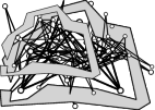
(b)

Figure 1: (a) A non-planar outside-obstacle representation of the octahedron; the obstacle is shown in gray. (b) A plane outside-obstacle representation of Figure 2(c).

Related Work. Graphs with an outside-obstacle representation are equivalent to visibility graphs of a pointset within a simple polygon. Therefore, polygon–vertex visibility graphs form an important subclass of our graphs class, where the pointset coincides with the corners of the surrounding simple polygon. Such graphs have been extensively studied due to their many applications, e.g., in gallery guarding [16].

Polygon–vertex visibility graphs were first introduced in 1983 by Avis and ElGindy [4] and are most studied in the field of visibility problems [13]. One of the first results on the topic was that maximal outerplanar graphs are polygon–vertex visibility graphs [8]. Ghosh [12] gives a set of four necessary conditions for polygon–vertex visibility graphs, which he conjectured to be also sufficient. However, Streinu [20] constructed a counterexample. As pointed out in [13], two of Ghosh’s necessary conditions [12] imply the conditions of a characterization attempt by Abello and Kumar in terms of oriented matroids [1], which hence cannot be sufficient.

So far, characterizations have only been achieved for polygon–vertex visibility graphs of restricted polygons. Everett and Corneil [10, 11] give a characterization of visibility graphs in spiral and 2-spiral polygons – polygons that have exactly one and two chains of reflex vertices, respectively. They are characterized as interval graphs and perfect graphs. The best known complexity result about the recognition and reconstruction problem of polygon–vertex visibility graphs is that they are in PSPACE [9].

A generalization of these graphs are induced subgraphs of polygon–vertex visibility graphs, or induced visibility graphs for short. Spinrad [19] considers this graph class the natural generalization of polygon–vertex visibility graphs, which is hereditary with respect to induced subgraphs. Everett and Corneil [11] show that there is no finite set of forbidden induced subgraphs in polygon–vertex visibility graphs.

Coullard and Lubiw show that 3-connected polygon–vertex visibility graphs admit a 3-clique ordering [6]. Abello et al. [2] prove that every 3-connected planar polygon–vertex visibility graph is maximal planar and that every 4-connected such graph cannot be planar. Their conjecture that Hamiltonian maximal planar graphs with a 3-clique ordering are polygon–vertex visibility graphs was disproven by Chen and Wu [5]. According to O’Rourke [17] necessary and sufficient conditions for a polygon–vertex visibility graph to be planar are known [14], but do not lead to a polynomial recognition algorithm.

For the more general question of obstacle numbers, Alpert et al. [3] give a construction for graphs with large obstacle number and small example graphs that have obstacle number greater than 1. They further show that every outerplanar graph admits a (non-planar) outside-obstacle representation, i.e., they are visibility graphs of pointsets inside simple polygons. Subsequent papers extend the results on obstacle numbers. Pach and Sarıöz [18] construct small graphs with obstacle number 2 and show that bipartite graphs with arbitrarily large obstacle number exist. Mukkamala et al. [15] show that there are graphs on $n$ vertices with obstacle number $\Omega(n/\log{n})$. It is an open question whether any graph with obstacle number 1 admits an outside-obstacle representation.

Contribution and Outline.

(a)

(b)

(c)

Figure 2: Graphs admitting (c) / not admitting (a,b) a plane outside-obstacle representation.

In this paper, we study plane outside-obstacle representations, where the drawing of $G$, without the obstacles, is free of crossings; see Fig. 1(b) for an example. Consider the graphs shown in Fig. 2. We will see that the first two graphs do not admit a plane outside-obstacle representation, whereas the last example has one. Note that the drawing in Fig. 2(a) is a (non-planar) outside-obstacle representation. Our main results are the following. (1) Every outerplanar graph whose inner faces are triangles admits a plane outside-obstacle representation. (2) A characterization of the biconnected graphs that admit a plane outside-obstacle representation. (3) A linear-time algorithm for testing whether a biconnected graph admits a plane outside-obstacle representation. As a side result, we obtain a simple combinatorial proof of ElGindy’s classical result that maximal outerplanar graphs are polygon–vertex visibility graphs [8].

Our paper is structured as follows. First, we derive a simple necessary condition on the structure of biconnected graphs that admit a plane outside-obstacle representation in Section 2. This restricts the class of graphs we have to consider and we derive some useful structural results about such graphs. Afterwards, in Section 3, we give a local description of plane outside-obstacle representations and, based on this, we derive a combinatorial characterization of the biconnected planar graphs that admit a plane outside-obstacle representation in terms of an orientation of a certain subset of edges. Using this characterization, we prove our main results in Section 4.

2 Inner-Chordal Plane Graphs

A graph with a fixed planar embedding is inner-chordal plane if any cycle $C$ of length at least 4 has a chord that is embedded in the bounded region of $\mathbb{R}^{2}\setminus C$; see Fig. 3. We first show that we can restrict our analysis to inner-chordal plane graphs.

Lemma 1

Graphs with a plane outside-obstacle representation are inner-chordal plane.

Proof

Let $G$ be a graph with a plane outside-obstacle representation, and assume it is not inner-chordal. Hence, there exists a cycle $C$ of length at least 4, whose interior does not contain a chord. Note that the obstacle lies outside of $C$ by definition. The cycle $C$ is embedded as the boundary of a simple polygon $P$ on at least four vertices. Since $P$ can be triangulated, there exists a pair of non-adjacent vertices $u$ and $v$ on $C$ such that the segment $uv$ is completely contained in $P$. Hence the obstacle cannot intersect $uv$, and thus $\{u,v\}\in E(G)$ by definition, contradicting our choice of $u$ and $v$.

(a)

(b)

(c)

Figure 3: (a) An inner-chordal graph. (b), (c) Chordal, but not inner-chordal, plane graphs.

Note that Lemma 1 shows immediately that the graph from Fig. 2(a) does not admit a plane outside-obstacle representation. Although this graph is chordal, it does not have a planar embedding that is inner-chordal. In the following, we consider only inner-chordal plane graphs. Note that, in particular, every inner face of an inner-chordal plane graph is a triangle. Moreover, an outerplanar graph is inner-chordal if and only if it is chordal, which is the case if and only if every inner face is a triangle.

Lemma 2

Let $G$ be an inner-chordal plane graph. Then, every inner vertex of $G$ has degree 3 and no two inner vertices are adjacent.

Proof

Since $G$ is inner-chordal, every inner face is necessarily a triangle. This implies that the neighbors of any inner vertex form a cycle. This cycle does not have an inner chord, and hence, since $G$ is simple and inner-chordal, it must have length 3. This implies that any inner vertex has degree 3. Moreover, it follows that the neighbors of any inner vertex $v$ must be incident to the outer face as they already have degree 3 in the neighborhood of $v$.

This description also gives rise to a certain tree that is associated with every biconnected inner-chordal graph. Let $G$ be a biconnected inner-chordal plane graph. A chord of $G$ is an edge that is not incident to the outer face but whose endpoints are incident to the outer face. Lemma 2 implies a decomposition of $G$ along its chords. Namely, we first remove all inner vertices. Each such removal transforms a 4-clique of $G$ into a triangular face; we mark each triangle that results from such a removal. The resulting graph $G^{\prime}$ is outerplanar and every inner face is a triangle. Now the weak dual $T^{\prime}$ of $G^{\prime}$ is a tree, where each node corresponds to a triangle of $G^{\prime}$. By marking the nodes of $T^{\prime}$ that correspond to a marked triangle, we obtain the construction tree $T$ of $G$, denoted $T(G)$. Note that each marked node of $T(G)$ corresponds to a 4-clique of $G$, whereas an unmarked node corresponds to a triangular face of $G$. We refer to these nodes as $K_{4}$- and $K_{3}$-nodes, respectively. The edges of $T(G)$ correspond bijectively to the chords of $G$. We refer to the vertices of $T(G)$ as nodes to distinguish them from the vertices of $G$. For a node $\tau$ of $T(G)$, we denote by $V_{\tau}$ the vertices of the corresponding triangle or 4-clique.

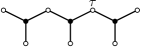
Figure 4: The construction tree of graphs (b) and (c) in Fig. 2; $K_{3}$-nodes are empty and $K_{4}$-nodes are filled. Structurally, the only difference between the two graphs is how the two subgraphs of $G$ are attached to the triangle corresponding to the $K_{3}$-node $\tau$.

Observe that, if we store with each node of $T(G)$ the corresponding edges and use the bijection of the edges of $T(G)$ with the chords of $G$ to find the shared chord of adjacent nodes, we can reobtain $G$ from $T(G)$ by merging triangles and 4-cliques that are adjacent in $T(G)$ along their shared chords. Then $T(G)$ is essentially the SPQR-tree of $G$ [7]. We decided to avoid the technical machinery associated with SPQR-trees and rather work with the construction tree, which is more tailored to our needs.

3 Characterization of Plane Visibility Representations

In this section we devise a combinatorial characterization of the biconnected inner-chordal graphs that admit a plane outside-obstacle representation. This is done in two steps. First, we show that, aside from being free of crossings, the property of being a plane outside-obstacle representation depends only on local features in the drawing, namely, for each chord of a graph $G$, its neighbors must be embedded in certain regions. In a second step, we show that this essentially induces a binary choice for each chord. In this way, an outside-obstacle orientation induces an orientation of the chords of $G$, and we will characterize the existence of a plane outside-obstacle representation in terms of existence of a suitable chord orientation.

Local Description of Plane Visibility Representations. Next we aim to understand better which planar straight-line drawings are outside-obstacle representations. As a first observation, consider two triangles $D$ and $D^{\prime}$ sharing a common edge $e=\{u,v\}$, which then forms a chord. Let $w$ and $w^{\prime}$ denote the tips of $D$ and $D^{\prime}$ with respect to base $e$, respectively. For an outside-obstacle representation it is a necessary condition that the non-edge $\{w,w^{\prime}\}$ intersects the outer face. We thus have to position the tips in such a way that the segments $ww^{\prime}$ does not lie inside the drawing of $D$ and $D^{\prime}$. We use the following definition; see Fig. 5(a) for an illustration.

Definition 1

Let $D$ be a triangle and $u$ a vertex of $D$. Then $R_{D}(u)$ denotes the intersection of the half-planes defined by the sides of $D$ incident to $u$ not containing $D$.

(a)

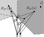
(b)

Figure 5: (a) Regions of triangle $D$ at edge $e=\{u,v\}$ and (b) attachment of two triangles $D$ and $D^{\prime}$ along chord $\{u,v\}$.

To ensure that the segment $ww^{\prime}$ intersects the outer face, it is clearly necessary that $w^{\prime}\in R_{D}(u)\cup R_{D}(v)$ or $w\in R_{D^{\prime}}(u)\cup R_{D^{\prime}}(v)$. The former ensures that the segment $ww^{\prime}$ does not intersect the interior of $D$ and the letter ensures the same property for $D^{\prime}$. These intersections behaviors are not independent. It is in fact readily seen that $w^{\prime}\in R_{D}(x)$ if and only if $w\in R_{D^{\prime}}(x)$ for $x\in\{u,v\}$; see Fig. 5(b). More generally, the same observations also hold for a chord $e=\{u,v\}$ that is shared by • (a) two triangles $\tau$ and $\tau^{\prime}$, (b) a triangle $\tau$ and a 4-clique $\tau^{\prime}$ and (c) by two 4-cliques $\tau$ and $\tau^{\prime}$. To see this, note that the regions $R_{D}(u)$ and $R_{D^{\prime}}(u)$ in Fig. 5(b) do not change if $D$ and/or $D^{\prime}$ are part of a 4-clique. More formally, let $W$ and $W^{\prime}$ be the vertices of $\tau$ and $\tau^{\prime}$ that are distinct from $u$ and $v$, respectively. Let $D$ and $D^{\prime}$ denote the triangles incident to $e$. Then the following condition is necessary

$$W^{\prime}\subseteq R_{D}(u)\text{\quad or \quad}W^{\prime}\subseteq R_{D}(v)\,\,.$$ (*)

Again it holds that $W^{\prime}\subseteq R_{D}(x)$ if and only if $W\subseteq R_{D^{\prime}}(x)$ for $x\in\{u,v\}$.

Given a planar straight-line drawing of a graph $G$, we say that a chord $e$ is good if its adjacent triangles or 4-cliques satisfy condition (* ‣ 3). This notion gives us a more local criterion to decide whether a given planar straight-line drawing is an outside-obstacle representation.

Lemma 3

Let $G$ be a biconnected inner-chordal plane graph and let $\Gamma$ be a planar straight-line drawing of $G$. Then $\Gamma$ is a (plane) outside-obstacle representation if and only if each chord is good.

Proof

The condition that each chord is good is necessary. For sufficiency we show that, in a drawing where each chord is good, every non-edge intersects the outer face.

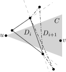
Figure 6: Illustration of the proof of Lemma 3.

Suppose for the sake of contradiction that $u$ and $v$ are two non-adjacent vertices of $G$ such that the segment $uv$ does not intersect the outer face. Then there is a minimal series $D_{1},\dotsc,D_{n}$ of adjacent triangles of $G$ such that the segment $uv$ is completely contained in the union of these triangles. Clearly, $n\geq 2$ and, without loss of generality, $u\in V(D_{1})$ and $v\in V(D_{n})$. We consider the subdrawing induced by $D_{1},\dots,D_{n}$. Since $uv$ intersects the triangle $D_{1}$, it intersects the edge of $D_{1}$ opposite of $u$, which implies that $v$ is contained inside the cone $C$ defined by $D_{1}$ with base $u$. We show that this contradicts statement $2$. If triangle $D_{i}$ for $1\leq i\leq n-1$ has the following properties: (i) its points are outside (or on the boundary) of $C$, (ii) the edge shared by $D_{i}$ and $D_{i+1}$ cuts across the cone $C$, and (iii) the line defined by the two points of $D_{i}$ that lie on the same side of $C$ slope away from $C$ in the direction towards $v$, then the very same properties hold for $D_{i+1}$ due to the chords being good; see Fig. 6. By definition the property holds for $D_{1}$, and hence it also holds for $D_{n}$. But this implies that the tip of $D_{n}$, which is $v$, must be placed outside of $C$, contradicting the assumption.

Unfortunately, it is not always possible to place the vertices inside the regions such that all chords become good as this placement may require crossings.

Chord Orientations and Outside-Obstacle Representations. Next, we introduce a certain type of orientations of the chords of biconnected inner-chordal graphs. Let $G$ be a biconnected inner-chordal graph and let $\Gamma$ be a plane outside-obstacle representation of $G$. Let $e=\{u,v\}$ be a chord of $G$, which exists, unless $G$ is $K_{3}$ or $K_{4}$. Let $D$ and $D^{\prime}$ denote the two triangles incident to $e$, and let $w$ and $w^{\prime}$ denote the tips of $D$ and $D^{\prime}$, respectively. Due to Lemma 3, each chord satisfies condition (* ‣ 3). Hence, either $w\in R_{D^{\prime}}(u)$ and $w^{\prime}\in R_{D}(u)$ or $w\in R_{D^{\prime}}(v)$ and $w^{\prime}\in R_{D}(v)$. We direct the chord $e$ towards $u$ in the former case and towards $v$ in the latter case. In this way, we obtain an orientation of the chords of $G$. Note that outer edges and inner edges of 4-cliques remain undirected. The following lemma shows two crucial properties of such an orientation.

Lemma 4

Let $G$ be a biconnected inner-chordal graph with plane outside-obstacle representation $\Gamma$. The chord orientation determined by $\Gamma$ satisfies the following properties.

1. Each vertex has in-degree at most 2.

2. If vertex $v$ has in-degree 2, then its two incoming edges share a face.

Proof

Consider an orientation according to $\Gamma$. Let $e=(u,v)$ be a directed chord with incident triangles $D$ and $D^{\prime}$, whose tips with respect to the base $e$ are $w$ and $w^{\prime}$, respectively. Due to the direction of $e$, we have that $w\in R_{D^{\prime}}(v)$ and $w^{\prime}\in R_{D}(v)$. It is readily seen, e.g., in Fig. 5(b), that the two angles at $v$ incident to $e$ sum up to more than $\pi$.

Let $e_{1},\dots,e_{k}$ be chords that are directed towards $v$. Without loss of generality assume that these chords are numbered in the order of counterclockwise occurrence around $v$, starting from the outer face. Since the angles at $v$ incident to each of these edges sum up to more than $\pi$, it follows that some of these angles must coincide. Due to the ordering, it follows that the angle at $v$ right of $e_{i}$ (with respect to the orientation towards $v$) coincides with the left angle of $e_{i+1}$ for $i=1,\dots,k-1$. By planarity and since $v$ is an outer vertex, no other angles may coincide. For $i=1,\dots,k$, let $\alpha_{i}$ denote the angle left of $e_{i}$ and let $\alpha_{k+1}$ denote the angle right of $e_{k}$. By the above observation, we have $\alpha_{i}+\alpha_{i+1}>\pi$ for $i=1,\dots,k$.

For $k\geq 3$, the sum of inner angles incident to $v$ is at least $\alpha_{1}+\alpha_{2}+\alpha_{3}+\alpha_{4}>2\pi$; a contradiction. For $k=2$ the shared angle $\alpha_{2}$ implies property (ii).

By virtue of Lemma 4, we call any orientation of the chords of a biconnected inner-chordal graph that satisfies the properties (i) and (ii) an outside-obstacle orientation.

Lemma 4 finally allows us to give a concise argument why the graph from Fig. 2(b) does not admit a plane outside-obstacle representation. We argue that it does not admit an outside-obstacle orientation. It follows from the conditions of such an orientation that, for each 4-clique that is incident to three chords, these chords must be oriented such that they form a cycle. Consider the middle 4-clique in Fig. 2(b). If we orient it clockwise, then the lower left edge may not have additional incoming chords, which prevents us from orienting the chords of the left 4-clique as a cycle. Symmetrically, choosing a counterclockwise orientation for the middle 4-clique prevents correct orientation of the right 4-clique. The graph in Fig. 2(c), however, does admit an outside-obstacle orientation, which is indicated in the figure.

Our next goal is to prove that the existence of an outside-obstacle orientation is equivalent to the existence of a plane outside-obstacle representation. In particular, this shows our claim that the graph in Fig. 2(c) indeed admits a plane outside-obstacle representation, e.g., the one shown in Fig. 1(b).

Theorem 3.1

Let $G$ be a biconnected inner-chordal plane graph. Then $G$ admits a plane outside-obstacle representation if and only if it admits an outside-obstacle orientation.

Proof

The “only if”-part holds due to Lemma 4. Let $G$ be a biconnected inner-chordal graph with an outside-obstacle orientation and let $T(G)$ be its construction tree. We construct a plane outside-obstacle representation of $G$.

For a subtree $T^{\prime}\subseteq T$, we denote by $G(T^{\prime})$ the subgraph of $G$ corresponding to $T^{\prime}$. Note that $G(T)=G$. Let $\tau_{1},\dots,\tau_{k}$ denote the nodes of $T$ in breadth-first order starting at an arbitrary node $\tau_{1}$. For $j=1,\dots,k$, let $T_{j}$ be the subtree of $T$ consisting of nodes $\tau_{1},\dots,\tau_{j}$, and let $G_{j}=G(T_{j})$ the corresponding subgraph of $G$. We inductively construct a sequence of plane outside-obstacle representations $\Gamma_{1},\dots,\Gamma_{k}$ of $G_{1},\dots,G_{k}$. Then $\Gamma_{k}$ is the desired plane outside-obstacle representation of $G=G_{k}$.

Consider the orientation of $G_{i}$ induced by $G$ (note that some edges remain undirected). We call a directed edge active if it is incident to the outer face of $G_{i}$ and inactive otherwise. An outer vertex $v$ is active if it is the target of an active edge. It is inactive otherwise. The inactive degree of $v$ in $G_{i}$ is the number of inactive edges with target $v$.

Throughout steps $i=1,\dots,k$, we maintain the following properties:

1. The outer angle of vertices with inactive degree 0 is convex.

2. For an active vertex $v$ with inactive degree 1, removing the unique active in-edge incident to $v$ results in a convex outer angle.

For $G_{1}$ any plane outside-obstacle representation $\Gamma_{1}$ satisfies these properties. We now show how to proceed from $G_{i}$ to $G_{i+1}$. Let $e=(u,v)$ be the directed chord determined by adding $\tau_{i+1}$ to $T(G_{i})$, let $D$ be the inner triangle of $G_{i}$ bounded by $e$ and let $e^{\prime}=(u^{\prime},v)$ denote the other edge of $D$ incident to $v$.

We aim to place the vertices in $V(G_{i+1})\setminus V(G_{i})$ inside the region $R_{D}(v)$, which is consistent with the orientation of $e$. We first show that this is possible without creating intersections. If $v$ has inactive degree 0, then $v$ is convex, and hence the intersection of $R_{D}(v)$ with a suitably small $\varepsilon$-ball around $v$ is disjoint from any vertices and edges of $\Gamma_{i}$. Similarly, if $v$ is active but has inactive degree 1, then, after removing $(u,v)$, $v$ is convex by property (ii). In this case the subcone of $R_{D}(v)$ defined by $e^{\prime}$ and the other outer edge incident to $v$ intersected with a suitably small $\varepsilon$-ball is empty; see Fig. 7(a).

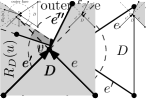
(a)

(b)

(c)

Figure 7: Construction of a plane outside-obstacle representation. (a) Attaching at a vertex $v$ with inactive degree 1. The region where the new points are placed is shaded in dark gray. (b), (c) show that adding an edge preserves the properties required by the construction. The shaded region is the inner part of the drawing after removing the active edge; the outer angle at $v$ is convex.

We show that, by placing the new vertices in these regions suitably close to $v$, properties (i) and (ii) can be established for the resulting plane outside-obstacle representation $\Gamma_{i+1}$. First observe that placing the new vertices close enough to $v$ avoids touching or crossing any vertices and edges of $G_{i}$, i.e., $\Gamma_{i+1}$ is plane. Moreover, the addition only changes angles at $u$ and $v$, and hence all other vertices satisfy properties (i) and (ii) by virtue of the induction hypothesis.

Consider vertex $v$. In $G_{i+1}$ it has inactive degree at least 1 since $(u,v)$ is an inner edge. If the inactive degree of $v$ is 2, there is nothing to prove as $v$ must be inactive, since outside-obstacle orientations have in-degree at most 2. Hence assume that $v$ has inactive degree 1 and it is active. The properties of outside-obstacle orientations imply that there is a unique active edge directed towards $v$ in $G_{i+1}$ and it must be a neighbor of $e$. This edge is either the edge $e^{\prime}$ or the newly added outer edge $e^{\prime\prime}$ incident to $v$.

If $e^{\prime}$ is the incoming active edge at $v$, the outer angle at $v$ was convex in $\Gamma_{i}$, and hence any point in $R_{D}(v)$ results in an outer angle of less than $\pi$ after removing $e^{\prime}$; see Fig. 7(b). If $e^{\prime\prime}$ is the incoming active edge at $v$, the outer angle at $v$ in $\Gamma_{i+1}$ after removing $e^{\prime\prime}$ is the outer angle of $v$ in $\Gamma_{i}$, which is convex by the induction hypothesis; see Fig. 7(c).

In all cases vertex $v$ satisfies properties (i) and (ii). We show that, by positioning the new vertices close enough to $v$, we can also satisfy properties (i) and (ii) for $u$. First note that the inactive degree of $u$ does not change. If the inactive degree of $u$ is 2, there is nothing to prove. If the inactive degree of $u$ is 0 or 1, by placing the new vertices close to the line through $u$ and $v$, the angle between $e$ and the new outer edge incident to $u$ can be made arbitrarily small. Thus, if $u$ was convex in $\Gamma_{i}$, it remains so in $\Gamma_{i+1}$. And, by the same argument, if $u$ was convex in $\Gamma_{i}$ after removing the active edge incident to $u$, it remains so in $\Gamma_{i+1}$. Hence $\Gamma_{i+1}$ satisfies the induction hypothesis.

4 Characterization and Decision Algorithm

In this section, we prove characterizations of graphs that admit a plane outside-obstacle representation and we present a linear-time algorithm that decides whether a given graph admits a plane outside-obstacle representation.

Characterization of Outerplanar Graphs. For biconnected outerplanar graphs Theorem 3.1 immediately implies a complete characterization of the graphs that admit a plane outside-obstacle representation.

Theorem 4.1

A biconnected outerplanar graph admits a plane outside-obstacle representation if and only if it is chordal.

Proof

Being chordal is a necessary condition due to Lemma 1. Conversely, if an outerplanar graph is chordal, it is obviously inner-chordal. We show that every biconnected inner-chordal outerplane graph admits an outside obstacle orientation.

Recall that a biconnected outerplanar graphs contains a vertex of degree at most 2. We iteratively construct an orientation by directing the incident edges of a vertex with degree at most 2 towards it and removing it from the graph. In this way, we obtain an orientation with the properties that each vertex has in-degree at most 2, and moreover, if a vertex has in-degree 2, then the two incoming edges share an inner face. Undoing the orientations of the outer edges, we obtain an outside-obstacle orientation. Now the claim follows from Theorem 3.1.

This result can easily be strengthened in two ways. First, if the outerplanar graph is not biconnected but chordal, then it can easily be augmented such that it becomes biconnected but remains (inner-)chordal and outerplanar and hence satisfies the conditions of Theorem 4.1, yielding a plane outside-obstacle representation of the augmented graph. By iteratively removing augmentation edges that are incident to the outer face we obtain a plane outside-obstacle representation of the original graph.

Corollary 1

An outerplanar graph admits a plane outside-obstacle representation if and only if it is chordal.

Another observation is that the construction of the orientation in the proof of Theorem 4.1 essentially consists of a bottom-up traversal of the construction tree of the graph with respect to the root node, which is removed last. It is then readily seen that we can also remove $K_{4}$-nodes that are leaves, provided they have degree at most 2 in $T(G)$. A $K_{4}$ with degree 3 requires that its chords are oriented to form a cycle, which cannot be ensured by the construction. It can, however, always be achieved it the $K_{4}$ of degree 3 is the root of the tree. We thus have the following corollary.

Corollary 2

Every biconnected inner-chordal graph that contains at most one $K_{4}$ for which all outer edges are chords admits a plane outside-obstacle representation.

Note that an augmentation as in the proof of Corollary 2 may increase the number of $K_{4}$-nodes with degree 3. Hence the result does not extend to non-biconnected graphs.

Decision Algorithm for General Graphs. Next, we devise a linear-time algorithm to decide whether a biconnected graph admits a plane outside-obstacle representation. Of course it is not difficult to test whether a graph is inner-chordal and plane in linear time, and we assume in the following that our input graph has these properties.

Due to Theorem 3.1, deciding the existence of a plane outside-obstacle representation is equivalent to deciding the existence of an outside-obstacle orientation. To test whether a biconnected inner-chordal plane graph $G$ admits an outside obstacle orientation, we use dynamic programming on its construction tree $T(G)$, rooted at an arbitrary node.

For each node $\tau$ with parent edge $\{u,v\}$ with orientation $uv$ and binary flags $d_{\tau,u}$ and $d_{\tau,v}$, we are interested whether the subtree of $T(G)$ with root $\tau$ admits an outside-obstacle orientation such that

1. $\{u,v\}$ is oriented as $uv$,

2. $u$ has incoming edges if and only if $d_{\tau,u}=1$, and

3. $v$ has incoming edges distinct from $uv$ if and only if $d_{\tau,v}=1$.

We store this information in a 4-dimensional table $T[\tau,e,d_{\tau,u},d_{\tau,v}]$ of boolean variables. Note that, for each node $\tau$, table $T$ contains only $2^{3}=O(1)$ entries. We now show how to fill the entries of this table in linear time. Initially, we set all entries to false.

For a leaf node $\tau$ with parent edge $\{u,v\}$, we set $T[\tau,uv,0,0]=T[\tau,vu,0,0]=$ true, which models the fact that we can choose any orientation of $\{u,v\}$ and neither $u$ nor $v$ has incoming edges distinct from $\{u,v\}$ in the subtree consisting only of the leaf. Let $\tau$ be a node with children $\tau^{\prime}$ and $\tau^{\prime\prime}$ and corresponding chords $\{u,w\},\{v,w\}$ that connect them to $\tau$. We can easily check whether the entries can be combined to an entry of $\tau$. Namely, try both possible orientations of $\{u,v\}$ and use the orientations of $\{u,w\}$ and $\{v,w\}$ determined by the entries of the children and the flags $d_{\tau^{\prime},u}$, $d_{\tau^{\prime},w}$, $d_{\tau^{\prime\prime},v}$, and $d_{\tau^{\prime\prime},w}$ of the children to check that $u,v$ and $w$ satisfy the constraints of the orientation. If this is the case, we can easily compute the two flags $d_{\tau,u}$ and $d_{\tau,v}$ from the orientations of $uw$, $vw$ and the flags $d_{\tau^{\prime},u}$ and $d_{\tau^{\prime\prime},v}$. A simple induction shows that, in this way, we set exactly the correct entries $T[\tau,\cdot,\cdot,\cdot]$ to true.

Combining two entries takes $O(1)$ time. Since there are only $2^{3}=O(1)$ entries per node, we can compute all entries of a node $\tau$ from all combinations of entries of its at most two children in $O(1)$ time. Since there are $O(n)$ nodes, the overall algorithm runs in $O(n)$ time. At the root we may have to combine up to three children, but the checks remain essentially the same. Thus, the overall algorithm runs in $O(n)$ time.

Theorem 4.2

There is a linear-time algorithm that decides whether a given biconnected graph admits a plane outside-obstacle representation.

5 Conclusion

Inspired by obstacle representations introduced by Alpert et al. [3], we studied plane outside-obstacle representations of graphs. We characterized the biconnected graphs that admit such a representation as the inner-chordal graphs that admit a certain type of orientation of their chords. Based on this, we gave a combinatorial proof that every chordal outerplanar graph admits a plane outside-obstacle representation. We further derived a linear-time algorithm for deciding whether a given biconnected graph admits a plane outside-obstacle representation.

Our main open question are the following. Can our characterization and testing algorithm can be extended to general (inner-chordal) graphs that are not necessarily biconnected? Which graphs admit a plane representation with a single obstacle?

Acknowledgments Part of this work has been done while Alexander Koch participated in the academic exchange program of Tōhoku University and KIT. AK thanks Prof. Dorothea Wagner and Prof. Takeshi Tokuyama for their support and Prof. Yota Ōtachi from JAIST for helpful comments on the topic.

References

- [1] J. Abello and K. Kumar. Visibility graphs and oriented matroids. Discrete & Computational Geometry, 28:449–465, 2002.
- [2] J. Abello, H. Lin, and S. Pisupati. On visibility graphs of simple polygons. Congressus Numeratium, 90:119–128, 1992.
- [3] H. Alpert, C. Koch, and J. Laison. Obstacle numbers of graphs. Discrete & Computational Geometry, 44(1):223–244, 2010.
- [4] D. Avis and H. ElGindy. A combinatorial approach to polygon similarity. IEEE Transactions on Information Theory, 29(1):148–150, 1983.
- [5] C. Chen and K. Wu. Disproving a conjecture on planar visibility graphs. Theoretical Computer Science, 255:659–665, 2001.
- [6] C. Coullard and A. Lubiw. Distance visibility graphs. In Proceedings of the 7th Annual ACM Symposium on Computational Geometry (SOCG’91), pages 289–296. ACM Press, 1991.
- [7] G. Di Battista and R. Tamassia. On-line maintenance of triconnected components with SPQR-trees. Algorithmica, 15:302–318, 1996.
- [8] H. ElGindy. Hierarchical decomposition of polygons with applications. PhD thesis, McGill University, Montreal, 1985.
- [9] H. Everett. Visibility graph recognition. PhD thesis, TR 231/90, Department of Computer Science, University of Toronto, Ontario, Canada, 1990.
- [10] H. Everett and D. Corneil. Recognizing visibility graphs of spiral polygons. Journal of Algorithms, 11(1):1–26, 1990.
- [11] H. Everett and D. Corneil. Negative results on characterizing visibility graphs. Computational Geometry, 5(2):51–63, 1995.
- [12] S. Ghosh. On recognizing and characterizing visibility graphs of simple polygons. Discrete & Computational Geometry, 17(2):143–162, 1997.
- [13] S. Ghosh and P. Goswami. Unsolved problems in visibility graphs of points, segments and polygons. CoRR, abs/1012.5187, 2010.
- [14] S. Lin and C. Chen. Planar visibility graphs. Proceedings of the 6th Canadian Conference on Computational Geometry (CCCG’94), 1994.
- [15] P. Mukkamala, J. Pach, and D. Pálvölgyi. Lower bounds on the obstacle number of graphs. Electronic Journal of Combinatorics, 19(12):P32, 2012.
- [16] J. O’Rourke. Art Gallery Theorems and Algorithms. International Series of Monographs on Computer Science. Oxford University Press, 1987.
- [17] J. O’Rourke. Open problems in the combinatorics of visibility and illumination. Contemporary Mathematics, 223:237–244, 1998.
- [18] J. Pach and D. Sariöz. On the structure of graphs with low obstacle number. Graphs and Combinatorics, 27(3):465–473, 2011.
- [19] J. Spinrad. Efficient graph representations. Fields Institute monographs. AMS, 2003.
- [20] I. Streinu. Non-stretchable pseudo-visibility graphs. Computational Geometry: Theory and Applications, 31:195–206, 2005.