Determinant quantum Monte Carlo study of the two-dimensional single-band Hubbard-Holstein model

Abstract

We have performed numerical studies of the Hubbard-Holstein model in two dimensions using determinant quantum Monte Carlo (DQMC). Here we present details of the method, emphasizing the treatment of the lattice degrees of freedom, and then study the filling and behavior of the fermion sign as a function of model parameters. We find a region of parameter space with large Holstein coupling where the fermion sign recovers despite large values of the Hubbard interaction. This indicates that studies of correlated polarons at finite carrier concentrations are likely accessible to DQMC simulations. We then restrict ourselves to the half-filled model and examine the evolution of the antiferromagnetic structure factor, other metrics for antiferromagnetic and charge-density-wave order, and energetics of the electronic and lattice degrees of freedom as a function of electron-phonon coupling. From this we find further evidence for a competition between charge-density-wave and antiferromagnetic order at half-filling.

I Introduction

The electron-phonon ($e$-$ph$ ) interaction is at the heart of a number of important phenomena in solids. It can be a dominant factor in determining transport properties or produce broken symmetry states such as conventional superconductivityBCS ; Migdal1 and/or charge-density-wave (CDW) order.GrunerRMP1988 In systems well described by Fermi liquid theory, many of these phenomena are understood within the framework of Migdal and Eliashberg theory, which provides a quantitative account of this physics.Migdal1 ; Migdal2 ; Eliashberg The situation however can be quite different in correlated systems where the role of the $e$-$ph$ interaction is far less well understood, sometimes even on a qualitative level.

From an experimental point of view, interest in the $e$-$ph$ interaction in correlated systems has largely been driven by research on transition metal oxides, and in particular the high-T_c cuprates. For example, in undoped Ca_2-xNa_xCuOCl₂, angle-resolved photoemission spectroscopy (ARPES) studies have found broad gaussian spectral features which have been interpreted in terms of Franck-Condon processes and polaron physics.ShenPRL2004 This is supported by models for a single hole coupled to the lattice and doped into an antiferromagnetic background,BoncaPRB2008 ; CataudellaPRL2007 ; MishchenkoPRL2004 which reproduce the observed lineshape and dispersion. Similarly, the structure of the optical conductivity of the undoped cuprates is well reproduced by models with strong (polaronic) $e$-$ph$ coupling.MishchenkoPRL2008 ; DeFilippisPRB2009 These observations point towards a strong $e$-$ph$ interaction in the undoped and underdoped cuprates, where strong correlations have the largest effect.

Evidence for lattice coupling also exists in the doped cuprates. Perhaps the most discussed are the dispersion renormalizations in the nodal and anti-nodal regions of the Brillouin zone revealed by ARPES.CukPRL2004 ; LanzaraNature2001 ; KordyukPRL2006 ; JohnsonPRL2001 ; VishikPRL2012 ; PlumbPRL2010 ; DahmNaturePhysic2009 ; JohnstonACMP2010 These manifest as sharp changes or “kinks” in the electronic band dispersion, which are generally believed to be due to coupling to a sharp bosonic mode. Although the identity of this mode (be it an electronic collective mode or one or more phonon modes) remains controversial, the appearance of the dispersion renormalizations at multiple energy scales ranging from 10 - 110 meV strongly suggests coupling to a spectrum of oxygen phonons.VishikPRL2012 ; PlumbPRL2010 ; LeePRB2008 ; AnzaiPRL2010 ; RameauPRB2009 ; MeevasanaPRL2006 These electronic renormalizations have analogous features in the density of states as probed by scanning tunnelling microscopyLeeNature2006 ; Pasupathy ; JenkinsPRL2009 ; deCastroPRL2008 ; ZasadzinskiPRL2006 ; ZhuPRB2006 ; JohnstonDOS ; GuomengZhao as well as in the optical properties of the cuprates.CarbotteReview ; EvH

Moving beyond the cuprates, strong $e$-$ph$ and electron-electron ($e$-$e$ ) interactions also are believed to be operative in a number of other systems. These include the quasi-1D edge-shared cuprates,LeePreprint the manganites, MillisNature1998 ; MillisPRB1996 ; MannellaPRB2007 , the fullerenes,Durand2003 ; CaponeScience2002 ; GunnarssonRMP1997 ; HanPRL2003 and the rare-earth nickelates.MedardeJPCM1997 ; LauPreprint Thus understanding the role of the $e$-$ph$ interaction in correlated systems is an important problem with possible implications across many materials families.

One of the primary barriers to resolving these issues is the incomplete understanding of how the direct interplay between the $e$-$ph$ interaction and other important degrees of freedom (such as strong $e$-$e$ interactions, magnetic degrees of freedom, reduced dimensionality, charge localization, etc.) influences the $e$-$ph$ interaction. On quite general grounds one expects that competition and/or cooperative effects can significantly alter the nature of the $e$-$e$ and $e$-$ph$ interactions. Strong $e$-$e$ interactions will suppress charge fluctuations and will have a tendency to localize carriers and renormalize the $e$-$ph$ interaction. Conversely, the $e$-$ph$ interaction mediates a retarded attractive interaction between electrons that can counteract the repulsive Coulomb interaction. However, the interaction with the lattice will further dress quasiparticle mass, producing heavier quasiparticles which may be affected more significantly by the $e$-$e$ interaction. In the limit of strong coupling this can lead to small polaron formation which also localizes carriers. In the end which, if any, of these effects wins out is a complicated question.

Recent work has begun to examine these issues by incorporating the Coulomb interaction at varying levels using a variety of analytical and numerical methods. This has resulted in a number of interesting results which are sometimes contradictory. Recent Fermi-liquid based treatments of the long-range components of the Coulomb interaction have shown that the $e$-$ph$ coupling constant can be significantly enhanced at small momentum transfers due to the quasi-2D nature of transport in the cuprates and the breakdown of screening in the deeply underdoped samples. AlexandrovPRL2011 ; AlexandrovPRB1996 ; JohnstonPRB2010 ; JohnstonPRL2012 ; MeevasanaScreening ; MeevasanaPRL2006 The enhanced coupling in the forward scattering direction can enhance pairing in a $d$-wave superconductorBulutPRB1996 and also affects the energy scale of the dispersion renormalization.MaksimovPRB2005 The modification of the $e$-$ph$ vertex appears to be generic as studies examining the short-range components of the Coulomb interaction as captured by the Hubbard interaction find similar forward scattering enhancements of the $e$-$ph$ vertex.KulicPRB1994 ; HuangPRB2003 ; ZeyherPRB1996 The short-range Hubbard interaction may also impact the energy scale of the $e$-$ph$ renormalizations in the electronic dispersion as evidenced by a recent dynamical mean-field theory (DMFT) study.BauerPRB2010

Cooperative and competitive effects between the two interactions also have been examined in the limit of strong correlations. One example of this is in the context of understanding the anomalous broadening and softening of the Cu-O bond stretching phonon modes in the high-T_c cuprates as a function of doping.Pintschovius ; ReznikNature Attempts to account for the observed renormalizations within density functional theory have generally been unsuccessful, particularly in the case of the phonon linewidth.DFT ; ReznikNature In contrast, correlated multiband and $t$-$J$ models with phonons have experienced more success in describing this physics.HorschPhysicaB2005 ; RoschPRB2004 The most likely origin of this discrepancy is the underestimation of correlations and the over-prediction of screening effects within DFT.

The presence of multiple interactions is also expected to enhance quasiparticle masses and therefore influence the formation of small polarons. DMFT studies of the Hubbard-Holstein (HH) model have found that the Hubbard interaction modifies the critical coupling $\lambda_{c}$ for the crossover to a small polaron.MishchenkoPRL2004 ; MacridinPRL2006 ; BoncaPRB2008 ; RoschPRB2004 However, the suppression or enhancement of $\lambda_{c}$ depends on the underlying phase: paramagnetic (suppression) or antiferromagnetic (enhancement).SangiovanniPRL2005 ; SangiovanniPRL2006 These results indicate the importance of correlations and the presence of the underlying magnetic order. A Diagrammatic Monte Carlo work on the $t$-$J$-Holstein model also found an increased tendency towards polaron formation for a single hole doped into an AFM background.MishchenkoPRL2004 Similar results have been obtained in other approaches applied to $e$-$ph$ coupling in $t$-$J$ models,BoncaPRB2008 ; RoschPRB2004 ; RoschPRL2004 ; MishchenkoPRL2004 ; Prelovsek however these results are in contrast with the exact solution for a two-site HH model where $\lambda_{c}$ increases for increasing Hubbard interaction strengths.BerciuPRB2007 Although this result was obtained for a small molecular cluster, it does highlight the need to examine models where $U$ is finite in order to allow for the possible destabilization of the AFM correlations by the $e$-$ph$ interaction. Without this effect it is impossible to address the competition between AFM and a competing order driven by the $e$-$ph$ interaction, such as superconductivity or CDWs, in an unbiased manner.

In the case of the HH model the $e$-$ph$ and $e$-$e$ interactions can drive competition between different ordered phases. Take for example the half-filled Hubbard and Holstein models on a two dimensional square lattice. The single-band Hubbard model has strong ${\bf Q}=(\pi/a,\pi/a)$ correlations which favor single occupation of the sites.WhitePRB1989 Conversely, the single-band Holstein model exhibits a ${\bf Q}=(\pi/a,\pi/a)$ CDW phase transition at finite temperature.ScalettarPRB1989 ; MarsiglioPRB1990 In the CDW ordered phase the lattice sites are doubly occupied in a checkerboard pattern. When both interactions are present the tendency towards these incompatible orders clearly will compete.BauerPRB2010_2 ; BauerEPL2010 ; FehskePRB2004 ; ClayPRL2005 ; NowadnickPRL2012 Competing orders in correlated systems is a prominent issue and a common theme in many transition metal oxides where novel physics often emerges at the boundary between orders.

The $T=0$ phase diagrams of the half-filled HH model in one and infinite dimensions have been mapped out.BauerPRB2010_2 ; BauerEPL2010 ; FehskePRB2004 ; ClayPRL2005 Recently this work was extended and a finite temperature phase diagram was proposed for the two-dimensional (2D) case at half-filling using determinant quantum Monte Carlo (DQMC).NowadnickPRL2012 Fig. 1 sketches the result, extending the diagram shown in Fig. 4 of Ref. NowadnickPRL2012, to include additional metrics for the phases involved. In Fig. 1a the average value of the double occupancy is shown as a function of the $e$-$e$ ($U$) and $e$-$ph$ ($\lambda$, dimensionless units, see below) interaction strengths. When the $e$-$e$ interaction dominates AFM correlations develop and $\langle n_{\uparrow}n_{\downarrow}\rangle$ is small. Conversely, when the $e$-$ph$ interaction dominates $\langle n_{\uparrow}n_{\downarrow}\rangle$ tends towards $0.5$ as half of the sites are doubly occupied in a ${\bf Q}=(\pi/a,\pi/a)$ checkerboard pattern. These limits are divided by the line where the strength of the $e$-$e$ interactions is comparable to the $e$-$ph$ interaction (indicated by the red line), which is taken to be the approximate phase boundary.

This phase diagram is quite similar to the ones drawn for the one- and infinite- dimensional cases, however, in the vicinity of the transition there is debate as to whether there is an intervening metallic state. Here, in the finite $T$ 2D case, we find indications of such a phase.NowadnickPRL2012 This is most clearly seen in the spectral weight at the Fermi level, which is related to $G(\tau=\beta/2)$NowadnickPRL2012 and is shown in Fig. 1b. To the left (right) of transition region spectral weight is suppressed at the Fermi level due to the opening of a Mott (CDW) gap. However, in the transition region the spectral weight is maximal, consistent with an intervening metallic phase. The point of maximal spectral weight lays near the line where $\langle n_{\uparrow}n_{\downarrow}\rangle=0.25$, a value equal to that expected for a paramagnetic metal. Furthermore, as the temperature is lowered, the low energy spectral weight in the intervening phase grows, indicative of metallic behavior, while the spectral weight in the large $U$ and $\lambda$ regimes falls, as expected for an insulator NowadnickPRL2012 . These results are in contrast to the results obtained in infinite dimensions and $T=0$ where a first order AFM/CDW transition has been proposed.BauerPRB2010_2 ; BauerEPL2010 At this stage it is unclear what role dimension and temperature are playing, indicating the need for further studies.

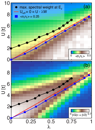
Figure 1: (color online) The finite temperature ($\beta=4/t$) phase diagrams for the two-dimensional Hubbard-Holstein model at half-filling. The vertical axis is the strength of the Hubbard interaction while the horizontal axis is the strength of the Holstein interaction measured in dimensionless units (see text). The color scale in the upper panel gives the average value of the double occupancy per site. In the lower panel it gives the spectral weight at the Fermi surface. For reference, the point of maximum spectral weight is shown in the upper panel and the line where the double occupancy is one quarter is shown in the lower panel. The red line indicates the line where $U_{\mathrm{eff}}=0$ in the antiadiabatic limit.

In this paper we apply DQMC to study the 2D single-band HH model. DQMC is a non-perturbative auxiliary-field technique capable of handling both the Hubbard and Holstein interactions on equal footing. This is particularly important if one wishes to address competition between the two interactions in an unbiased manner. Our results show a number of indications of a competition between the ${\bf Q}=(\pi/a,\pi/a)$ CDW and AFM orders. The primary evidence for this has been reported in a previous letter (Ref. NowadnickPRL2012, ). The purpose of this work is to outline the algorithm, benchmark it, and present supporting evidence for the competition between CDW and AFM in the half-filled model. Results are given for the fermion sign, which is important for assessing when and where it is feasible to apply DQMC. For large $e$-$e$ interactions the fermion sign problem generally restricts DQMC simulations to high temperature however, we find a parameter regime with strong $e$-$e$ and $e$-ph interactions where the fermion sign recovers. This opens the possibility of treating strongly correlated polarons at finite carrier concentrations provided the phonon field sampling remains efficient.

The organization of this work is as follows. In the following section we will briefly review the DQMC method as it applies to the HH model. As previous worksWhitePRB1989 ; BSS have outlined the method in the context of the Hubbard model, here we focus on the additional aspect associated with the treatment of the lattice degrees of freedom. Following this we begin presenting results. Section III examines the severity of the fermion sign problem throughout parameter space. Section IV examines the filling and compressibility of the model as a function of chemical potential. These results are intended to provide a reference point for future finite concentration studies. From this point forward we then restrict ourselves to half-filling. In section V we study the AFM structure factor and metrics for the AFM & CDW orders as a function of $e$-$ph$ coupling. These results provide further evidence of the competition between the two orders at half-filling. This competition also is evident in the energetics of the electronic and lattice degrees of freedom which are presented in section VI. Finally, in section VII we summarize and make some concluding remarks.

II Formalism

In this section we outline the DQMC algorithm. The general approach follows the original formalism of Refs. WhitePRB1989, and BSS, . Here we briefly summarize the method and highlight the changes and additions required to handle the lattice degrees of freedom.

II.1 The Hubbard-Holstein Model

The HH hamiltonian is a simple model capturing the physics of itinerant electrons with both $e$-$e$ and $e$-$ph$ interactions. In this model the motion of the lattice sites is described by a set of independent harmonic oscillators at each site $i$, with position and momentum operators $\hat{X}_{i}$ and $\hat{P}_{i}$, respectively. The $e$-$e$ and $e$-$ph$ interactions are both treated as local interactions – the $e$-$e$ interaction given by the usual Hubbard interaction while the $e$-$ph$ interaction arises from the linear coupling of the local density to the atomic displacement $\hat{X}_{i}$. The HH hamiltonian can be decomposed into $H=H_{el}+H_{lat}+H_{int}$ where

$$H_{el}=-t\sum_{\langle i,j\rangle,\sigma}c_{i,\sigma}^{{\dagger}}c^{\phantom{\dagger}}_{j,\sigma}-\mu\sum_{i,\sigma}\hat{n}_{i,\sigma},$$ (1)

and

$$H_{lat}=\sum_{i}\left(\frac{M\Omega^{2}}{2}\hat{X}_{i}^{2}+\frac{1}{2M}\hat{P}^{2}_{i}\right),$$ (2)

contain the non-interacting terms for the electron and lattice degrees of freedom, respectively, and

$$H_{int}=U\sum_{i}\left(\hat{n}_{i,\uparrow}-\frac{1}{2}\right)\left(\hat{n}_{i,\downarrow}-\frac{1}{2}\right)-g\sum_{i,\sigma}\hat{n}_{i,\sigma}\hat{X}_{i}$$ (3)

contains the interaction terms. Here, $c^{\dagger}_{i,\sigma}$ ($c_{i,\sigma}^{\phantom{\dagger}}$) creates (annihilates) an electron of spin $\sigma$ at site $i$, $\hat{n}_{i,\sigma}=c^{\dagger}_{i,\sigma}c^{\phantom{\dagger}}_{i,\sigma}$ is the number operator, $\langle\dots\rangle$ denotes a sum over nearest neighbors, $t$ is the nearest neighbor hopping, $\Omega$ is the phonon frequency, $U$ and $g$ are the $e$-$e$ and $e$-$ph$ interaction strengths, respectively, and $\mu$ is the chemical potential, adjusted to maintain the desired filling. It is convenient to define the dimensionless $e$-$ph$ coupling $\lambda=g^{2}/(M\Omega^{2}W)$, equal to the ratio of the lattice deformation energy $E_{p}=g^{2}/(2M\Omega^{2})$ to half the non-interacting bandwidth $W/2\sim 4t$. Throughout this work we use $\lambda$ as a measure of the $e$-$ph$ coupling strength and set $a=M=t=1$ as the units of length, mass and energy, respectively.

The competition between the Hubbard and Holstein interactions is often demonstrated by explicitly integrating out the phonon degrees of freedom. After which one obtains an effective dynamic Hubbard interactionBergerPRB1995

$$U_{\mathrm{eff}}(\omega)=U+\frac{g^{2}}{M(\omega^{2}-\Omega^{2})}=U-\frac{W\lambda}{1-(\omega/\Omega)^{2}}.$$ (4)

The second term represents the retarded attractive interaction mediated by the phonons for $\omega<\Omega$. In the antiadiabatic limit $\Omega\rightarrow\infty$ with $\lambda$ held fixed, this interaction becomes instantaneous and one is left with an effective Hubbard model with $U_{\mathrm{eff}}=U-g^{2}/M\Omega^{2}=U-\lambda W$. For large values of $\Omega$ the behavior the HH model approaches that of the $U_{\mathrm{eff}}$ model. However, for small $\Omega$, retardation effects can become important as observed in comparisons between the HH and $U_{\mathrm{eff}}$ Hubbard models when one examines observables such as the CDW and AFM susceptibilities.NowadnickPRL2012 ; SangiovanniPRL2005 Nevertheless, the frequency-independent $U_{\mathrm{eff}}$ model is used often to describe the HH model and recent studies have found that some of the low-energy properties of the model can be captured by such an approximation.SangiovanniPRL2005 ; BauerEPL2010

II.2 The DQMC Algorithm

In general, one wishes to evaluate the finite temperature expectation value of an observable $\hat{O}$ given by

$$\langle\hat{O}\rangle=\frac{{\mathrm{Tr}\hat{O}e^{-\beta H}}}{\mathrm{Tr}e^{-\beta H}}$$ (5)

where the averaging is performed within the grand canonical ensemble. In order to evaluate Eq. (5), the imaginary time interval $[0,\beta]$ is divided into $L$ discrete steps of length $\Delta\tau=\beta/L$. The partition function can then be rewritten using the Trotter formula as Suzuki

$$Z=\mathrm{Tr}(e^{-\Delta\tau LH})=\mathrm{Tr}(e^{-\Delta\tau H_{int}}e^{-\Delta\tau K})^{L},$$ (6)

where $K$ is the matrix form of the non-interacting terms $K=H_{el}+H_{lat}$, and terms of order $tU(\Delta\tau)^{2}$ and higher have been neglected. In many other modern QMC approaches this Trotter error is eliminated by using continuous time algorithms.GullRMP However, with DQMC one has a highly efficient sampling scheme which is difficult to implement in a continuous time approach. We will return to this point when we discuss Monte Carlo updates. For our choice of discrete time grids the Trotter errors are typically a few percent and difficult to discern against the background of statistical errors when evaluating long range correlation and structure factors.

With this discrete imaginary time grid the Hubbard interaction terms can now be written in a bilinear form by introducing a discrete Hubbard-Stratonovich field $s_{i,l}=\pm 1$ at each site $i$ and time slice $l$. This results in

$$e^{-\Delta\tau U(\hat{n}_{i,\uparrow}-1/2)(\hat{n}_{i,\downarrow}-1/2)}=A\sum_{s_{i,l}=\\ \pm 1}e^{-\Delta\tau s_{i,l}\alpha(\hat{n}_{i,\uparrow}-\hat{n}_{i,\downarrow})}$$ (7)

where $A=\frac{1}{2}e^{-\Delta\tau U/4}$ and $\alpha$ is defined by the relation $\cosh(\Delta\tau\alpha)=\exp(\Delta\tau U/2)$ HS ; BSS ; WhitePRB1989 . In the absence of the $e$-$ph$ interaction, the trace over fermion degrees of freedom can be performed and the partition function is expressed as a product of determinants BSS

$$Z=\sum_{s_{i,l}}\det{M_{\uparrow}}\det{M_{\downarrow}}$$ (8)

where $M^{\sigma}=I+B^{\sigma}_{L}B^{\sigma}_{L-1}\dots B^{\sigma}_{1}$. Here $I$ is an $N\times N$ identity matrix and the $B_{l}$ matrices are defined as

$$B_{l}^{\uparrow(\downarrow)}=e^{\mp\Delta\tau\alpha v(l)}e^{-\Delta\tau K},$$ (9)

where $v(l)$ is a diagonal matrix whose $i$-th element is the field value $s_{i,l}$. The evaluation of Eq. (8) now requires a Monte Carlo averaging of the auxiliary fields $s_{i,l}$ (see section IIC). This expression must be modified when introducing the $e$-$ph$ interaction.

In order to handle the motion of the lattice, the position operator $\hat{X}_{i}$ is replaced with a set of continuous variables $X_{i,l}$ defined on the same discrete imaginary time grid as the Hubbard-Stratonovich fields. The momentum operator is replaced with a finite difference $P_{i,l}=M(X_{i,l+1}-X_{i,l})/\Delta\tau$ and periodic boundary conditions are enforced on the interval $[0,\beta]$ such that $X_{i,L}=X_{i,0}$. In this treatment we recover the proper values for the average phonon kinetic and potential energy in the non-interacting limit provided the sampling of the phonon displacements has been done with care.

With these changes the fermion trace can again be performed and one has

$$Z=\int dX\sum_{s_{i,l}}e^{-E_{ph}\Delta\tau}\det{M_{\uparrow}}\det{M_{\downarrow}}$$ (10)

where $\int dX$ is short hand for integrating over all of the continuous phonon displacements $X_{i,l}$ and $M^{\sigma}$ is defined as before but with modified matrices

$$B_{l}^{\uparrow(\downarrow)}=e^{\mp\Delta\tau\alpha v(l)-\Delta\tau gX(l)}e^{-\Delta\tau K}.$$ (11)

The matrix $v(l)$ is defined as before and $X(l)$ is a diagonal matrix whose $i$-th diagonal element is $X_{i,l}$. The factor $\exp(-E_{ph}\Delta\tau)$ arises from the bare kinetic and potential energy terms of the lattice Hamiltonian, $H_{lat}$, where

$$E_{ph}=\frac{M\Omega^{2}}{2}X^{2}_{i,l}+\frac{M}{2}\left(\frac{X_{i,l+1}-X_{i,l}}{\Delta\tau}\right)^{2}.$$ (12)

An expression for the numerator of Eq. (5) can be obtained in an analogous way.

Most observables can be expressed in terms of the single-particle Green’s function $G^{\sigma}(\tau)$. For an electron propagating through field configurations $\{s_{i,l}\}$, $\{X_{i,l}\}$, the Green’s function at time $\tau=l\Delta\tau$ is given byWhitePRB1989

$$[G^{\sigma}(l)]_{ij} = \langle\hat{T}_{\tau}c^{\phantom{\dagger}}_{i,\sigma}(\tau)c^{\dagger}_{j,\sigma}(\tau)\rangle$$

$$= [I+B_{l}^{\sigma}\dots B_{1}^{\sigma}B_{L}^{\sigma}\dots B_{l+1}^{\sigma}]^{-1}_{ij},$$

where ${\hat{T}_{\tau}}$ is the time ordering operator. The determinant of $M^{\sigma}$ appearing in Eq. (10) is independent of $l$ and is related to the Green’s function on any time slice $G_{\sigma}(l)$ by $\mathrm{det}M^{\sigma}=\mathrm{det}G^{-1}(l)$.

II.3 Sampling the Auxiliary fields

The sampling of the Hubbard-Stratonovich and phonon fields is performed using two types of single-site updates as well as a “block” update for the phonon fields. In our implementation each Monte Carlo step consists of cycling through these three types.

II.3.1 Hubbard-Stratonovich Field Updates

The evaluation of Eq. (II.2) requires $O(N^{3})$ operations. However, once the Green’s function $G^{\sigma}(l)$ is known, the Green’s function on the next imaginary time slice can be efficiently computed with a set of matrix multiplications (an order $O(N^{2})$ operation)

$$G^{\sigma}(l+1)=B^{\sigma}_{l+1}G^{\sigma}(l)[B^{\sigma}_{i+1}]^{-1}.$$ (14)

This forms the basis for an efficient single site update scheme. One begins by computing the Green’s function on a single time slice using Eq. (II.2). A series of updates are then proposed for the Hubbard-Stratonovich fields while holding the current configuration $\{X_{i,l}\}$ fixed. This portion follows the prescription given in Ref. WhitePRB1989, . One sweeps through all sites $i$ proposing $s_{i,l}\rightarrow-s_{i,l}=s_{i,l}^{\prime}$, which is accepted with probability

$$R=R^{\uparrow}R^{\downarrow}=\frac{\mathrm{det}M^{\uparrow\prime}\mathrm{det}M^{\downarrow\prime}}{\mathrm{det}M^{\uparrow}\mathrm{det}M^{\downarrow}},$$ (15)

where $M^{\sigma\prime}$ and $M^{\sigma}$ correspond to the HS fields with and without the proposed update, respectively.

Since the phonon fields are held fixed during this update, fast Sherman-Morrison updates can be performed in the usual manner.WhitePRB1989 One has

$$B^{\sigma}(l)\rightarrow B^{\sigma\prime}(l)=[I+\Delta^{\sigma}(i,l)]B^{\sigma}(l)$$ (16)

where the matrix $[\Delta^{\sigma}(i,l)]_{jk}=\delta_{ik}\delta_{ik}[\exp(\pm 2\Delta\tau s_{i,l})-1]$ has a single non-zero element. The ratio of determinants can be computed easily from

$$R^{\sigma}=1+(1-[G^{\sigma}(l)]_{ii})[\Delta^{\sigma}(i,l)]_{ii}.$$ (17)

If the spin-flip of the Hubbard-Stratonovich field is accepted, the updated Green’s function is given by

$$[G^{\sigma}(l)]^{\prime}=G^{\sigma}(l)-\frac{G^{\sigma}(l)\Delta^{\sigma}(i,l)[I-G^{\sigma}(l)]}{1+[1-G_{ii}^{\sigma}(l)]\Delta^{\sigma}_{ii}(i,l)}.$$ (18)

$\Delta^{\sigma}(i,l)$ has a single non-zero element, making evaluation of Eq. (18) straightforward. Once updates have been performed for all fields on time slice $l$, $G^{\sigma}(l)$ is advanced to $G^{\sigma}(l+1)$ using Eq. (14) and the process repeated.

This update scheme is efficient however, it cannot be fully exploited in an auxiliary field continuous time approach where one defines time slices $\tau_{i}$ on a variable grid with spacing $\Delta\tau_{i}=\tau_{i+1}-\tau_{i}$ and sampling is performed over the auxiliary fields and number of time slices. For a fixed number of time slices the methodology outline above holds and the fast update scheme can be used. The difficulty enters when one proposes the insertion or removal of a time slice from the set. These updates are accepted with a probability related to the ratio of determinants similar to Eq. (15) times an additional prefactor to satisfy detailed balance.GullRMP However, the new configuration in this case involves a different number of time slices and thus the determinants must be computed from scratch, which is computationally expensive. Since continuous time approaches require many of these types of updates we choose to remain on a discrete grid where fast sampling of the auxiliary fields can be maintained on larger clusters.

II.3.2 Phonon Field Updates

Single-site updates for the phonon fields proceed in a manner analogous to that for the Hubbard-Stratonovich fields. For each point $(i,l)$ one proposes updates $X_{i,l}\rightarrow X^{\prime}_{i,l}=X_{i,l}+\Delta X_{i,l}$ while holding the configuration $\{s_{i,l}\}$ fixed. In this case $\Delta X_{i,l}$ is drawn from a box probability distribution function. The proposed phonon update is then accepted with probability $R=R^{\uparrow}R^{\downarrow}\exp(-\Delta\tau\Delta E_{ph})$ where $\Delta E_{ph}$ is the total change in kinetic and potential energy associated with the update, and $R^{\sigma}$ is defined by Eq. (15). The $\Delta E_{ph}$ term accounts for the contribution of $H_{lat}$ to the total action. The fast Sherman-Morrison update scheme can also be performed for single-site phonon updates with $\Delta^{\sigma}(i,l)$ replaced by

$$[\Delta^{\sigma}(i,l)]_{jk}=\delta_{ik}\delta_{jk}[\exp(-\Delta\tau\Delta X_{i,l})-1].$$ (19)

II.3.3 Block Updates for the Phonon Fields

As noted previously, sampling the phonon fields requires some additional care. In addition to the single-site update scheme we have found that a block update scheme is necessary to reproduce correct results in the non-interacting and atomic limits. In this update scheme the lattice position for a given site is updated such that $X_{i,l}\rightarrow X_{i,l}+\Delta X$ for all $l\in[0,L]$.ScalettarPRB1991 This type of update helps to efficiently move the phonon configurations out of false minima at lower temperatures. However, it comes at a price. Block updates spanning multiple imaginary time slices are computationally expensive within the DQMC formalism. They require that the Green’s function be recalculated from scratch since updates are being made on multiple time slices simultaneously. This is an $O(N^{3})$ operation in contrast to the $O(N^{2})$ cost of Eq. (18). Therefore a balance between the two types of phonon updates must be struck. As a rule of thumb we have found that two to four block updates at randomly selected sites for every full set of single site updates to $\{s_{i,l}\}$ and $\{X_{i,l}\}$ is sufficient to recover the correct behavior in the non-interacting and atomic limits. In our implementation $\Delta X$ is drawn from a separate box probability distribution function.

III The Fermion Sign

We begin with the average value of the fermion sign, which is the limiting factor for any QMC treatment of correlated electrons. In Fig. 2 we focus on the average sign at half-filling as a function of $e$-ph coupling for a moderately correlated case ($U=4t$). Results are shown for a phonon frequency $\Omega=t$ and inverse temperature $\beta=8/t$. Since we have only included nearest neighbour hopping, the average sign at half-filling is protected by particle-hole symmetry for $\lambda=0$.WhitePRB1989 This protection results from the fact that although $\mathrm{det}M_{\sigma}<0$, symmetry dictates $\mathrm{sign}(\mathrm{det}M_{\uparrow})=\mathrm{sign}(\mathrm{det}M_{\downarrow})$ in a particle-hole symmetric system; thus the ratio $R$ remains positive definite. This no longer holds for finite $e$-$ph$ coupling since most phonon configurations $\{X_{i,l}\}$ break this symmetry leading to a sign problem at half-filling. Increasing $\lambda$ suppresses the average sign until reaching a minimum that depends on the cluster size. For larger clusters this minimum persists over a wide range of $\lambda$; however, the average sign eventually recovers in all cases when $W\lambda\gtrsim U$. This behavior is generic for all parameter sets we have examined at half-filling and is due to the strong reduction of $U_{\mathrm{eff}}$ produced by the attractive interaction mediated by the $e$-$ph$ interaction. This result indicates that although simulations of the HH model at low $T$ remain limited by the fermion sign problem for arbitrary parameter ranges, this need not be true for simulations of the correlated polaronic regime (large $\lambda$ with moderate to large $U$).

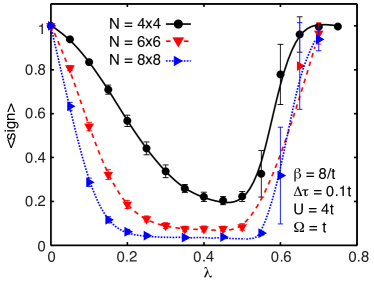
Figure 2: (color online) The average value of the fermion sign as a function of $e$-$ph$ coupling $\lambda$ for various half-filled clusters. The parameters for these calculations are $\beta=8/t$, $\Delta\tau=t/10$, $U=4t$, and $\Omega=t$

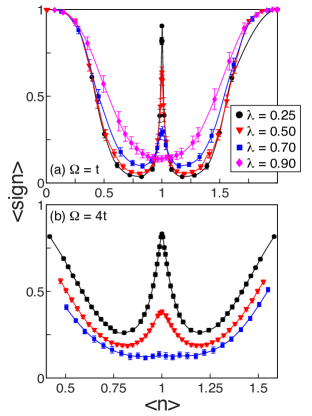
Figure 3: (color online) The average value of the fermion sign as a function of filling for $\lambda=0.25$ ($\circ$), $0.5$ ($\triangledown$), $0.7$ ($\square$), and $0.9$ ($\diamond$). Results are shown for two sets of phonon frequencies $\Omega=t$ (panel a) and $\Omega=4t$ (panel b). All data sets are for the strongly correlated limit with $U=8t$. These results were obtained on a $N=8\times 8$ cluster with $\Delta\tau=0.1/t$. The inverse temperatures for panels (a) and (b) are $\beta=4/t$ and $3/t$, respectively. The solid lines are guides to the eye.

Turning to finite carrier concentrations, Fig. 3 shows the average sign as a function of filling for a strongly correlated system ($U=8t$), phonon frequencies $\Omega=t$ (Fig. 3a) and $\Omega=4t$ (Fig. 3b) (the latter being closer to the antiadiabatic limit), and inverse temperatures are $\beta=4/t$ and $3/t$, respectively. For weak $e$-ph coupling doping suppresses the sign in a manner similar to the bare Hubbard model WhitePRB1989 where the most severe sign problem occurs near $\langle n\rangle\sim 0.85$ and $\sim 1.15$. Upon increasing $\lambda$, the behavior at half-filling follows that shown in Fig. 2. However, at finite doping, the evolution of the fermion sign depends on the phonon frequency. For $\Omega=t$ the average value of the sign increases with the inclusion of the $e$-$ph$ interaction for most carrier concentrations away from the immediate vicinity of half filling. Conversely, for $\Omega=4t$, the average sign is systematically suppressed and a deep minimum develops over a wide doping range for the largest values of $\lambda$ considered. This indicates that the way in which the $e$-$ph$ coupling affects the sign problem depends both on the strength of the effective attraction as well as retardation effects. We will return to this point shortly. Fig. 3 also shows that for large $\lambda$, the degree to which the sign is enhanced or suppressed at finite doping is comparatively smaller than the size of the induced sign problem at half filling. In other words, although a sign problem is induced at half-filling, it does not appear to be significantly exacerbated, and can even be improved by the $e$-$ph$ interaction, near carrier concentrations that are of interest for the doped high-T_c cuprates.

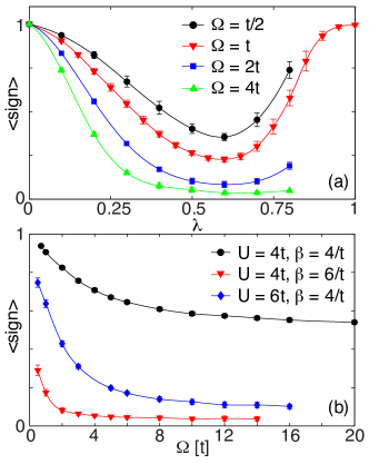
Figure 4: (color online) (a) The average sign for $\langle n\rangle=1$ as a function of $\lambda$ for $\Omega=t/2$ ($\circ$), $t$ ($\triangledown$), $2t$, ($\square$), and $4t$ ($\vartriangle$). The Hubbard interaction strength is held fixed at $U=6/t$, and the inverse temperature is $\beta=4/t$. (b) The average value of the fermion sign at half-filling as a function of the phonon frequency $\Omega$ and fixed $e$-$ph$ coupling $\lambda=0.25$. Results are shown for $U=4t$,$\beta=4/t$ ($\circ$), $U=4t$, $\beta=6/t$ ($\triangledown$), and $U=6t$, $\beta=4/t$ ($\Diamond$). All results in panels (a) and (b) were obtained on an $N=8\times 8$ clusters with $\Delta\tau=0.1/t$.

The $\Omega$ dependence of the average sign reinforces the notion that the degree of retardation associated with the $e$-$ph$ interaction plays an important role in determining the dressing of the Hubbard interaction. To explore this further in Fig. 4a we show the average sign at half-filling for $t/2<\Omega<4t$ as a function of $\lambda$. For a given value of $\Omega$ the overall trend remains similar to Fig. 2, however, increasing $\Omega$ results in a greater overall suppression of the average sign, indicating that $U$ is suppressed more rapidly by antiadiabatic phonons. The opposite trend was observed in the AFM susceptibilities, where AFM was suppressed at lower values of $\lambda$ for larger $\Omega$.NowadnickPRL2012 This suggests that the fermion sign is influenced both by the magnitude of $U$ and the degree of retardation encoded in $U_{\mathrm{eff}}(\omega)$.auto This possibility is underscored by contrasting the instantaneous $U_{\mathrm{eff}}$ model to the HH model with large $\Omega$. In the $U_{\mathrm{eff}}$ model particle-hole symmetry holds and the average value of the sign is identically one. In contrast, we observe that the sign is lower for $\Omega$ approaching the antiadiabatic limit as shown in Fig. 4b for a fixed $\lambda=1/4$. Futhermore, the average sign is suppressed more rapidly for small $\Omega$ before asymptotically approaching a $U$- and $\beta$-dependent value at high frequency. We interpret the value of the sign at large $\Omega$ as the size of the induced sign problem introduced by the breaking of particle-hole symmetry by the phonon fields. A possible explanation for the improved sign at small $\Omega$ is the attractive $e$-$ph$ -mediated interaction for electrons at the Fermi level. Recall that the dynamic effective Hubbard interaction introduced by the phonons $U^{ph}_{\mathrm{eff}}(\omega)$ is attractive for $\omega<\Omega$ and, and divergent for $\omega\rightarrow\Omega$. Thus as the phonon frequency tends to smaller values, a significant suppression of the repulsive Hubbard interaction occurs for electrons in a window near the Fermi level. If the average sign is determined primarily by electrons in this window then one would expect the sign to be improved. Further work is clearly needed to clarify this interesting possibility.

IV Filling and Compressibility

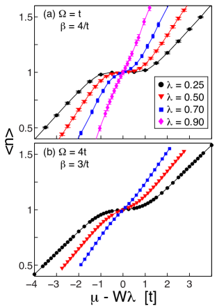
Figure 5: (color online) The average value of the filling $\langle n\rangle$ as a function of chemical potential $\mu-W\lambda$ for the same parameter sets shown in Fig. 3. The $-W\lambda$ correction accounts for the global shift of the lattice equilibrium position (see main text).

Fig. 5 shows the average filling on an $8\times 8$ cluster as a function of chemical potential $\mu$ for the same parameter set used to obtain the results shown in Fig. 3. (A chemical potential shift $\Delta\mu=-W\lambda$ due to the equilibrium lattice position has been subtracted off such that $\mu=-0$ corresponds to half-filling, see appendix A.) Fig. 6 shows the corresponding compressibility $\kappa\propto\frac{\partial\langle n\rangle}{\partial\mu}$ for the system.FootNote1 In these results one starts to see indications of competition between the attractive interaction mediated by the $e$-ph interaction and the repulsive $e$-$e$ interaction. For small values of $\lambda$ the strong Hubbard interaction ($U=8t$) dominates, opening a Mott gap in the system which clearly manifests as a plateau in $\langle n(\mu)\rangle$ and incompressibility $\kappa\sim 0$ located near $\mu-W\lambda=0$. As the strength of the $e$-ph interaction increases the effective attractive interaction grows. This reduces the influence of the Hubbard interaction and the size of the Mott gap begins to diminish. This is evident in the shrinking width of the plateau in $\langle n(\mu)\rangle$ and the rise in the value of $\kappa$. In the limit of large $\lambda$ all indications of the Mott gap vanish and $\langle n(\mu)\rangle$ behaves in a manner expected for a metallic state. The system has a finite compressibility and $\kappa\rightarrow 0$ as the band completely fills. This qualitative behavior occurs for both phonon frequencies and is further evidence for the direct competition between the attractive $e$-$ph$ interaction and repulsive $e$-$e$ interaction discussed in Ref. NowadnickPRL2012, . For this parameter set, $\lambda\sim 1$ marks the position where one expects the transition between the AFM and CDW order (see Fig. 1). We interpret this as further evidence for an intervening metallic state between the two orders at finite temperature. Finally, for the largest coupling $\lambda=0.9$ the $\kappa\rightarrow 0$ for $\mu-W\lambda\rightarrow 3t$ indicating that the total bandwidth of the system has been narrowed by the interactions present in the system.

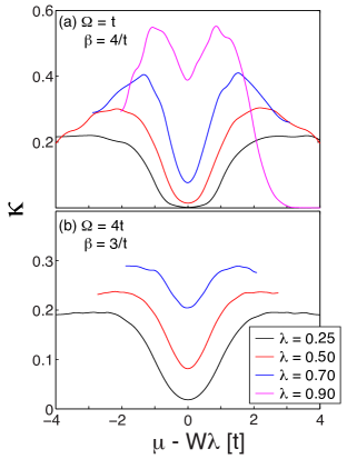
Figure 6: (color online) The compressibility $\kappa$ as a function of chemical potential for the same parameter set shown in Fig. 5.FootNote1

V Charge-density-wave and Antiferromagnetic Correlations

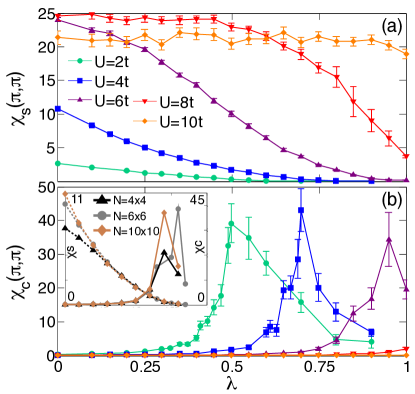
Figure 7: (color online). The (a) spin $\chi_{s}(\pi,\pi)$ and (b) charge $\chi_{c}(\pi,\pi)$ susceptibilities for several values of U on an $N=8\times 8$ cluster, reproduced from Ref. NowadnickPRL2012, . The inset of (b) shows $\chi_{s}$ (dashed lines) and $\chi_{c}$ (solid lines) at $U=4t$ for several lattice sizes. The error bars in the inset have been suppressed for clarity. The remaining parameters are $\beta=4/t$, $\Delta\tau=0.1/t$, and $\Omega=t$.

In this section we address the issue of competition between the $e$-$ph$ -driven CDW and $e$-$e$ -driven AFM correlations for the model at half-filling. We begin by first reviewing our previous results for the charge $\chi_{c}({\bf q})$ and spin $\chi_{s}({\bf q})$ susceptibilities, defined as

$$\chi_{s,c}({\bf q})=\frac{1}{N}\int_{0}^{\beta}d\tau\langle T_{\tau}\hat{O}^{\phantom{\dagger}}_{s,c}({\bf q},\tau)\hat{O}_{s,c}^{\dagger}({\bf q},0)\rangle,$$ (20)

where $\hat{O}_{s}({\bf q})=\sum_{i}e^{i{\bf q}\cdot{\bf R_{i}}}(\hat{n}_{i,\uparrow}-\hat{n}_{i,\downarrow})$, and $\hat{O}_{c}({\bf q})=\sum_{i,\sigma}e^{i{\bf q}\cdot{\bf R_{i}}}\hat{n}_{i,\sigma}$.

Our results for $\chi_{s}(\pi,\pi)$ and $\chi_{c}(\pi,\pi)$ are reproduced in Fig. 7 as a function of $\lambda$ and for several values of $U$.NowadnickPRL2012 For increasing $e$-$ph$ coupling, $\chi_{s}$ (Fig. 7a) is suppressed as a result of the reduction in the effective Hubbard interaction. For small values of $U$, $\chi_{s}$ is suppressed immediately for finite $\lambda$. However, for larger values of $U$, where more robust AFM correlations are present, $\chi_{s}$ persists up to $\lambda\sim U/W$ before beginning a significant drop as a function of $\lambda$. (This is seen most clearly in the data for $U=8t$.) At the same time, as $\lambda$ increases there is a corresponding increase in $\chi_{c}(\pi,\pi)$ (Fig. 7b). This occurs gradually at first while $\chi_{s}$ is large, but once the AFM correlations have been suppressed sufficiently there is a sharp increase in the growth of $\chi_{c}$. This indicates a competition between the two orders as the AFM correlations must be suppressed before charge ordering can occur. Finally, for $U\leq 6t$, further increases in $\lambda$ result in a decreasing $\chi_{c}$. We interpret this as being due to the finite CDW transition temperature in the HH model.NowadnickPRL2012 The inset of Fig. 7 shows similar results obtained on different lattices, demonstrating that the finite size effects do not qualitatively alter this picture.

Another measure of the AFM correlations in the single-band model can be obtained from the magnitude of the equal-time spin structure factor $S(\pi,\pi)$, which is defined as the Fourier transform of the spin-spin correlation function $c(l_{x},l_{y})$ WhitePRB1989

$$S({\bf q})=\sum_{\bf l}e^{i{\bf q}\cdot{\bf l}}c(l_{x},l_{y})$$ (21)

where ${\bf l}=(l_{x},l_{y})$ is the lattice position and

$$c(l_{x},l_{y})=\frac{1}{N}\sum_{{\bf i}}\langle(\hat{n}_{{\bf i}+{\bf l},\uparrow}-\hat{n}_{{\bf i}+{\bf l},\downarrow})(\hat{n}_{{\bf i},\uparrow}-\hat{n}_{{\bf i},\downarrow})\rangle.$$

Here the sum over ${\bf i}$ has been introduced to average over translationally equivalent quantities as opposed to a non-trivial spatial sum as in Eq. (21).

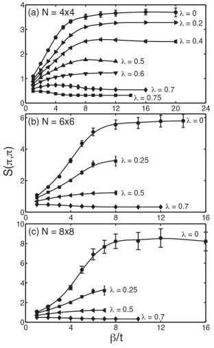
Figure 8: The structure factor $S(\pi,\pi)$ as a function of inverse temperature $\beta$ for the half-filled Hubbard-Holstein model. Results are shown for clusters of linear dimension (a) $N=4$, (b) $N=6$, and (c) $N=8$ and for several values of the electron-phonon coupling strength $\lambda$, as indicated. The remaining parameters are $U=4t$, $\Delta\tau=0.1t$, and $\Omega=t$.

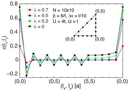
Figure 9: (color online) The real space structure of the spin-spin correlation function $c(l_{x},l_{y})$ along the path indicated in the inset. For $\lambda=0$ (black $\triangledown$) the antiferromagnetic correlations are evident. For increasing values of $\lambda$ the antiferromagnetism is suppressed. By $\lambda=0.5$ (blue $\triangle$), where $\lambda W\sim U$, all traces of antiferromagnetic correlations are gone.

In Fig. 8 we plot the structure factor $S(\pi,\pi)$ at the antiferromagnetic ordering vector for a series of half-filled clusters with $U=4t$. The data are plotted as a function of inverse temperature and for various values of the $e$-$ph$ coupling strength, as indicated in the figure. The $\lambda=0$ results well reproduce the results of White et al. WhitePRB1989 for the Hubbard model. However, the suppression of the AFM correlations as a function of $\lambda$ is apparent and $S(\pi,\pi)$ is reduced over the entire temperature range for finite values of $\lambda$. The suppression of the AFM order is also evident in the structure of the real space spin-spin correlation function $c(l_{x},l_{y})$, as shown in Fig. 9. The results for $\lambda=0$ show a clear staggered moment in the real space spin structure. However, for $\lambda=0.7$, which is below the peak in the CDW susceptibility (see Fig. 7b), the spin correlations resemble the result obtained in the paramagnetic metallic state.WhitePRB1989 This behavior is also reflected in the real-space density correlation function, shown in Fig. 10 for the same parameter set. For weak $e$-$ph$ coupling the cluster has a uniform charge distribution however upon increasing $\lambda$ to $0.7>U/W$ a clear ($\pi,\pi$) charge-density-wave forms. The behavior of both of these correlation functions implies the presence of an intervening metallic state below the onset of the CDW transition.

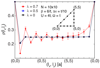
Figure 10: (color online) The real space structure of the density-density correlation function along the path indicated in the inset. For $\lambda=0$ (black $\triangledown$) the density of the system is uniform within error bars. This uniform density persists for increasing values of $\lambda\leq 0.5$ (blue $\triangle$). However, for $\lambda=0.7>U/W$ (red $\square$) a $(\pi,\pi)$ charge-density-wave correlation begins to develop.

VI Energetics at half-filling

In this final section we present results for the energetics of the lattice and electronic degrees of freedom. Again we restrict ourselves to half-filling and examine the energetics across the AFM/CDW transition. We first examine the average kinetic energy of the electrons $K_{el}$, which is defined as

$$K_{el}=\left\langle-t\sum_{\langle i,j\rangle,\sigma}c^{\dagger}_{i,\sigma}c^{\phantom{\dagger}}_{j,\sigma}\right\rangle.$$ (22)

Fig. 11 shows the negative of $K_{el}$ plotted as a function of $e$-$ph$ coupling and for values of $U$ between $4t$ and $10t$. For $\lambda=0$ charge fluctuations are suppressed by the Hubbard interaction and $-\langle K_{el}\rangle$ decreases for increasing values of $U$. As $\lambda$ increases the effective Hubbard interaction is lowered and $K_{el}$ decreases slowly as a function of $\lambda$. For reference, $K_{el}\sim-1.567t$ in the non-interacting limit. However, once $\lambda\sim U/W$ (indicated by the arrows) $K_{el}$ turns over and increases rapidly. The value of $\lambda$ at which this occurs coincides with both a pronounced change in the lattice potential energy (see below) and the onset of the CDW susceptibility.NowadnickPRL2012 In Ref. BauerPRB2010_2, similar behavior was observed in an assumed AFM ordered state.

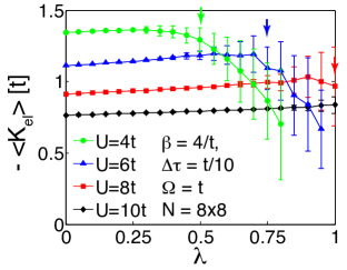
Figure 11: (color online) The negative of the average electron kinetic energy as a function of the $e$-$ph$ interaction strength $\lambda$ and $U=4t$ (green $\bigcirc$), $6t$ (blue $\triangle$), $8t$ (red $\square$), and $10t$ (black $\diamond$). The arrows indicate the value of coupling when $W\lambda=U$ for each data set.

The average potential energy of the electrons, which is proportional to the average number of doubly-occupied sites

$$\langle P_{el}\rangle=\left\langle\sum_{i}U\hat{n}_{i,\uparrow}\hat{n}_{i,\downarrow}\right\rangle,$$ (23)

is plotted in Fig. 12a. The average value of the double occupancy $\langle n_{\uparrow}n_{\downarrow}\rangle$ appears in Fig. 12b for reference. (The value for a non-interacting system is indicated by the dashed line.) Again one sees the apparent competition between the AFM and CDW orders. For $\lambda=0$ the system is dominated by the Hubbard interaction and the number of double-occupied sites is low and $P_{el}$ is lowered and for increasing $U$. When the $e$-$ph$ coupling increases $\langle n_{\uparrow}n_{\downarrow}\rangle$ grows. This happens slowly at small values of $\lambda$. However, once $\lambda\sim U/W$ the number of doubly-occupied sites grows more rapidly before saturating at a value of $0.5$ where half of the sites are doubly occupied as expected for ${\bf q}=(\pi,\pi)$ CDW order. Similarly, the electronic potential energy increases concomitantly with the increase in the cost of this double occupancy. This large cost in $P_{el}$ is compensated for by the gain in energy associated with the $e$-$ph$ interaction (see below).

The behavior of $\langle n_{\uparrow}n_{\downarrow}\rangle$ shown in Fig. 12 shows some differences from the results of infinite dimension DMFT.BauerPRB2010_2 Generically we see the growth in double occupancy occurring much more gradually than the DMFT result for the largest values of $U$. This appears to be the case regardless of the underlying state (charge ordered or normal) assumed in the DMFT calculations. One possible source for this difference is the presence of the intervening metallic state in two dimensions. If such a state were present one would expect to see $\langle n_{\uparrow}n_{\downarrow}\rangle$ flatten at $1/4$ as a function of $\lambda$ in this parameter regime. The thermal fluctuations present in our calculation would then broaden this to produce milder behavor like that shown here.

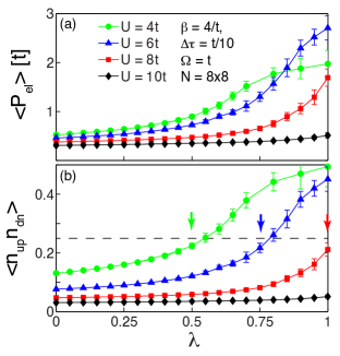
Figure 12: (color online) (a) The average potential energy of the electrons due to the Hubbard interaction $P_{el}$ as a function of $\lambda$ and $U=4t$ (green $\bigcirc$), $6t$ (blue $\triangle$), $8t$ (red $\square$), and $10t$ (black $\diamond$). (b) The corresponding average value of the double occupancy. The dash line indicates the value expected for the non-interacting metallic system. The arrows indicate the value of coupling when $W\lambda=U$ for each data set.

The average values of the phonon kinetic and potential energies are given by

$$\langle P_{ph}\rangle = \frac{M\Omega^{2}}{2}\left\langle\sum_{i,l}X^{2}_{i,l}\right\rangle$$ (24)

$$\langle K_{ph}\rangle = \frac{1}{2\Delta\tau}-\frac{M}{2}\left\langle\sum_{i,l}\bigg{(}\frac{X_{i,l+1}-X_{i,l}}{\Delta\tau}\bigg{)}^{2}\right\rangle.$$ (25)

The factor of $1/(2\Delta\tau)$ appearing in the kinetic energy term is a Euclidean correction introduced by the Wick rotation to the imaginary time axis. In the case of the lattice potential energy, we have subtracted off the contribution associated with the shift in the lattice equilibrium position in order to obtain a measure of the lattice fluctuations about equilibrium.

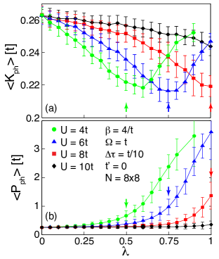
Figure 13: (color online) The average (a) kinetic and (b) potential energy of the lattice for the Hubbard-Holstein model as a function of the $e$-$ph$ interaction strength $\lambda$ and $U=4t$ (green $\bigcirc$), $6t$ (blue $\triangle$), $8t$ (red $\square$), and $10t$ (black $\diamond$).

The average values of the phonon kinetic and potential energies are shown in Figs. 13a and 13b, respectively, as a function of $\lambda$ and $U$. For $\lambda=0$ we recover the atomic result $\langle K_{ph}\rangle=\langle P_{ph}\rangle=\frac{\Omega}{2}[n_{b}(\omega)-1/2]$, where $n_{b}(\omega)=[\exp(\omega\beta)-1]^{-1}$ is the bose occupation number. For finite $e$-$ph$ coupling, the kinetic (potential) energy of the lattice slowly decreases (increases) for $\lambda\leq U/W$. This reflects a small renormalization of the phonons by scattering processes. A further increase in $\lambda$ crosses the transition point at which point the kinetic energy reaches a minimum before returning to a value comparable to that at $\lambda=0$ with a concomitant increase in the potential energy. Again, the minimum in $K_{ph}$ and onset in the $P_{ph}$ coincide with the peak in the CDW susceptibilities reported in Fig. 1b of Ref. NowadnickPRL2012, . Therefore these changes are linked to the onset of the CDW correlations and lattice’s checkerboard displacement pattern.

The total phonon energy is dominated by $P_{ph}$ and therefore the onset of the CDW correlations is marked by an accompanying increase in the electronic and lattice potential energy, consistent with the DMFT results in infinite dimensions. This is perhaps expected as the CDW state is associated with an increase in double occupied sites as well as large lattice distortions in the checkerboard arrangement. As previously mentioned, this energy comes from a corresponding gain in the $e$-$ph$ energy $E_{e-ph}=-\langle\sum_{i}gn_{i}X_{i}\rangle$ as shown in Fig. 14. As with the phonon potential energy, $E_{e-ph}$ shows a weak dependence for $\lambda<U/W$ which gives way to a rapid rise at the onset point of the CDW correlations.

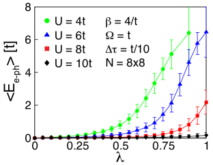
Figure 14: (color online) The average $e$-$ph$ interaction energy as a function of the $e$-$ph$ interaction strength $\lambda$ and $U=4t$ (green $\bigcirc$), $6t$ (blue $\triangle$), $8t$ (red $\square$), and $10t$ (black $\diamond$).

VII Concluding Remarks

We have presented the DQMC method applied to the two-dimensional HH model. In extending the DQMC algorithm to include lattice degrees of freedom we have found that care must be paid to the manner in which the phonon fields are sampled in order to ensure that one obtains the proper non-interacting limits. Once implemented, we benchmarked the algorithm and examined the severity of the fermion sign problem. Here we found that although the phonons introduce a sign problem where it was originally protected by particle-hole symmetry, they do not significantly change the value at finite carrier concentrations where DQMC typically performs poorly. This leaves open the possibility of examining carrier concentrations relevant to the high-T_c cuprates, which we leave for future work. We also found that the degree of retardation had a strong influence on the severity of the induced sign problem. However, we also observed a recovery of the fermion sign when $\lambda W\geq U$ and CDW correlations dominate. This suggests that parameter regimes corresponding to strongly correlated polarons may be accessible to DQMC.

Focusing on the half-filled model, we also presented further evidence for competition between the AFM and CDW ordered phases driven by the Hubbard and Holstein interactions, respectively. This work complements our previous findings,NowadnickPRL2012 and we see clear, systematic suppression of the AFM correlations as $\lambda$ increases. In all our metrics we found that for $\lambda W\sim U$ various quantities appear to be similar to the values one might expect for a metallic phase, providing further evidence in support of the presence of an intervening metallic phase between the CDW and AFM states, at least at high temperatures. Our results also indicate the importance of treating both interactions on equal footings. In the DQMC treatment, the $e$-$ph$ interaction is capable of destabilizing the AFM correlations and thus addressing true competition. This is not true for $t$-$J$-Holstein model treatments where a robust AFM persists for all values of $\lambda$. Thus one would like to revisit the issue of polaron formation using methods like the one presented here.

VIII Acknowledgements

S. J. and E. A. N. contributed equally to this work. We thank N. Nagaosa, A. S. Mishchenko, and N. Blümer for useful discussions. We acknowledge support from the U. S. Department of Energy, Office of Basic Energy Sciences, Materials Science and Engineering Division under Contract Numbers DE-AC02-76SF00515 and DE-FC0206ER25793. The work of R.T.S. was supported by the National Nuclear Security Administration under the Stewardship Science Academic Alliances program through DOE Research Grant #DE-NA0001842-0. S.J. acknowledges support from NSERC and SHARCNET (Canada). E.A.N. acknowledges support from the East Asia and Pacific Summer Institutes for U.S. Graduate Studies. Y.F.K. was supported by the Department of Defense (DoD) through the National Defense Science and Engineering Graduate Fellowship (NDSEG) Program and by the National Science Foundation Graduate Research Fellowship under Grant No. 1147470. The computational work was made possible in part by the facilities of SHARCNET and Compute Canada as well as the National Energy Research Scientific Computing Center (NERSC), which is supported by the Office of Science of the US Department of Energy under contract no. DE-AC02-05CH11231.

Appendix A Average Lattice Displacement

On warm-up the average value of the lattice position $X_{i,l}$ shifts to a non-zero equilibrium position. This is the result of the coupled system minimizing its energy by exploiting the $e$-$ph$ interaction energy at the expense of the lattice potential energy paid for the shifted equilibrium position. For a uniform charge density which one would expect for the half-filled case dominated by the Hubbard interaction, this lattice shift can be obtained by minimizing the total energy with respect to the phonon position. The new equilibrium position is given by

$$\frac{d}{dX}\left[\frac{M\Omega^{2}}{2}X^{2}-g\langle n\rangle X\right]=0$$ (26)

which for $\langle n\rangle=1$ yields $X=g/M\Omega^{2}=\sqrt{W\lambda}/\Omega$. In Fig. 15 we plot $\langle X\rangle$ as a function of $\lambda$ for $\Omega=t$ and $4t$. The data are well fit by the functional form $\langle X\rangle=\sqrt{W\lambda}/\Omega$ shown as the solid lines in the plot. This demonstrates that at half-filling the lattice shifts to a new equilibrium position and electrons couple to fluctuations around this point. This shift also accounts for the functional form of the renormalized chemical potential shift $\mu=-W\lambda$ used in Figs. 5 and 6.

Figure 15: (Color online) The average value of the lattice displacement $\langle X\rangle$ for the half-filled model as a function of $e$-ph coupling $\lambda$. Results are shown for $\Omega=t$ (red, $\circ$) and $\Omega=4t$ (blue $\square$). The remaining parameters are as indicated. The solid lines are of the form $\langle X\rangle=\sqrt{W\lambda}/\Omega$.

In general we have found that the DQMC algorithm begins to encounter numerical instabilities for phonon frequencies well into the adiabatic limit. The shift in equilibrium position is one of the possible sources for this instability - as the average lattice displacement gets large numerical overflows in the multiplication of the $B$ matrices begin to occur due to the exponential dependence in $X_{i,l}$. This difficulty could be overcome by writing the interaction term in the form $\sum_{i,\sigma}g(n_{i,\sigma}-\langle n\rangle)X_{i}$ provided the expectation value of the filling is known and the charge density is uniform. At half-filling such a procedure would be easy to implement however for finite doping a self-consistency loop would have to be built into the warm-up procedure. Furthermore, this procedure would likely do little to help in the CDW ordered phases once the average filling per site alternates from zero and two.

References

- (1) B. Bardeen, J. Copper, and J. R. Schrieffer, Phys. Rev. 108, 1175 (1957).
- (2) D. J. Scalapino in Superconductivity, edited by R. D. Parks (Dekker, New York, 1969), Vol. 1.
- (3) G. Grüner, Rev. Mod. Phys. 60, 1129 (1988).
- (4) A. B. Migdal, Soviet Physics JETP 34, 996 (1958).
- (5) G. M. Eliashberg, JETP 11, 696 (1960).
- (6) K. M. Shen, F. Ronning, D. H. Lu, W. S. Lee, N. J. C. Ingle, W. Meevasana, F. Baumberger, A. Damascelli, N. P. Armitage, L. L. Miller, et al., Phys. Rev. Lett. 93, 267002 (2004); K. M. Shen, F. Ronning, W. Meevasana, D. H. Lu, N. J. C. Ingle, F. Baumberger, W. S. Lee, L. L. Miller, Y. Kohsaka, M. Azuma, et al., Phys. Rev. B 75, 075115 (2007).
- (7) J. Bonča, S. Maekawa, T. Tohyama, and P. Prelovšek, Phys. Rev. B 77, 054519 (2008).
- (8) V. Cataudella, G. De Filippis, A. S. Mishchenko, and N. Nagaosa, Phys. Rev. Lett. 99, 226402 (2007).
- (9) A. S. Mishchenko and N. Nagaosa, Phys. Rev. Lett. 93, 036402 (2004).
- (10) A. S. Mishchenko, N. Nagaosa, Z.-X. Shen, G. De Filippis, V. Cataudella, T. P. Devereaux, C. Bernhard, K. W. Kim, and J. Zaanen, Phys. Rev. Lett. 100, 166401 (2008).
- (11) G. De Filippis, V. Cataudella, A. S. Mishchenko, C. A. Perroni, and N. Nagaosa, Phys. Rev. B 80, 195104 (2009).
- (12) T. Cuk, F. Baumberger, D. H. Lu, N. Ingle, X. J. Zhou, H. Eisaki, N. Kaneko, Z. Hussain, T. P. Devereaux, N. Nagaosa, and Z.-X. Shen, Phys. Rev. Lett. 93, 117003 (2004); T. P. Devereaux, T. Cuk, Z.-X. Shen, and N. Nagaosa, Phys. Rev. Lett. 93, 117004 (2004).
- (13) A. Lanzara, P. V. Bogdanov, X. J. Zhou, S. A. Kellar, D. L. Feng, E. D. Lu, T. Yoshida, H. Eisaki, A. Fujimori, K. Kishio, J. -I. Shimoyama, T. Noda, S. Uchida, Z. Hussain and Z. X. Shen. Nature 412, 510 (2001).
- (14) A. A. Kordyuk, S. V. Borisenko, V. B. Zabolotnyy, J. Geck, M. Knupfer, J. Fink, B. Büchner, C. T. Lin, B. Keimer, H. Berger, A. V. Pan, Seiki Komiya, and Yoichi Ando, Phys. Rev. Lett. 97, 017002 (2006).
- (15) P. D. Johnson, T. Valla, A. V. Fedorov, Z. Yusof, B. O. Wells, Q. Li, A. R. Moodenbaugh, G. D. Gu, N. Koshizuka, C. Kendziora, Sha Jian, and D. G. Hinks, Phys. Rev. Lett. 87, 177007 (2001).
- (16) T. Dahm, V. Hinkov, S. V. Borisenko, A. A. Kordyuk, V. B. Zabolotnyy, J. Fink, B. Büchner, D. J. Scalapino, W. Hanke, and B. Keimer, Nature Phys. 5, 217 (2009).
- (17) S. Johnston, W. S. Lee, Y. Chen, E. A. Nowadnick, B. Moritz, Z.-X. Shun, and T. P. Devereaux, Advances in Condensed Matter Physics 2010, 968304 (2010).
- (18) N. C. Plumb, T. J. Reber, J. D. Koralek, Z. Sun, J. F. Douglas, Y. Aiura, K. Oka, H. Eisaki, and D. S. Dessau, Phys. Rev. Lett. 105, 046402 (2010).
- (19) I. M. Vishik, W. S. Lee, F. Schmitt, B. Moritz, T. Sasagawa, S. Uchida, K. Fujita, S. Ishida, C. Zhang, T. P. Devereaux, and Z. X. Shen, Phys. Rev. Lett. 104, 207002 (2010).
- (20) W. S. Lee, W. Meevasana, S. Johnston, D. H. Lu, I. M. Vishik, R. G. Moore, H. Eisaki, N. Kaneko, T. P. Devereaux, and Z. X. Shen, Phys. Rev. B 77, 140504 (2008).
- (21) H. Anzai, A. Ino, T. Kamo, T. Fujita, M. Arita, H. Namatame, M. Taniguchi, A. Fujimori, Z.-X. Shen, M. Ishikado, and S. Uchida, Phys. Rev. Lett. 105, 227002 (2010).
- (22) J. D. Rameau, H.-B. Yang, G. D. Gu, and P. D. Johnson, Phys. Rev. B 80, 184513 (2009).
- (23) W. Meevasana, N. J. C. Ingle, D. H. Lu, J. R. Shi, F. Baumberger, K. M. Shen, W. S. Lee, T. Cuk, H. Eisaki, T. P. Devereaux, N. Nagaosa, J. Zaanen, and Z.-X. Shen, Phys. Rev. Lett. 96, 157003 (2006).
- (24) J. Lee, K. Fujita, K. McElroy, J. A. Slezak, M. Wang, Y. Aiura, H. Bando, M. Ishikado, T. Masui, J.-X. Zhu, et al., Nature (London) 442, 546 (2006)
- (25) A. N. Pasupathy, A. Pushp, K. K. Gomes, C. V. Parker, J. Wen, Z. Xu, G. Gu, S. Ono, Y. Ando, and A. Yazdani, Science 320, 196 (2008).
- (26) N. Jenkins, Y. Fasano, C. Berthod, I. Maggio-Aprile, A. Piriou, E. Giannini, B. W. Hoogenboom, C. Hess, T. Cren, and Ø. Fischer, Phys. Rev. Lett. 103, 227001 (2009).
- (27) J. F. Zasadzinski, L. Ozyuzer, L. Coffey, K. E. Gray, D. G. Hinks, and C. Kendziora, Phys. Rev. Lett. 96, 017004 (2006).
- (28) G. Levy de Castro, C. Berthod, A. Piriou, E. Giannini, and Ø. Fischer, Phys. Rev. Lett. 101, 267004 (2008).
- (29) J.-X. Zhu, A. V. Balatsky, T. P. Devereaux, Q. Si, J. Lee, K. McElroy, and J. C. Davis, Phys. Rev. B 73, 014511 (2006); J.-X. Zhu, K. McElroy, J. Lee, T. P. Devereaux, Q. Si, J. C. Davis, and A. V. Balatsky, Phys. Rev. Lett 97, 177001 (2006).
- (30) S. Johnston and T. P. Devereaux, Phys. Rev. B 81, 214512 (2010).
- (31) Guo-meng Zhao, Phys. Rev. B 75, 214507 (2007); Guo-meng Zhao, Phys. Rev. Lett. 103, 236403 (2009).
- (32) J. P. Carbotte, T. Timusk, and J. Hwang, Reports on Progress in Physics 74, 066501 (2011).
- (33) E. van Heumen, E. Muhlethaler, A. B. Kuzmenko, H. Eisaki, W. Meevasana, M. Greven and D. van der Marel, Phys. Rev. B 79, 184512 (2009).
- (34) W. S. Lee, S. Johnston, B. Moritz, J. Lee, M. Yi, K. J. Zhou, T. Schmitt, L. Patthey, V. Strocov, K. Kudo, Y. Koike, J. van den Brink, T. P. Devereaux, and Z. X. Shen, arXiv:1301.4267 (2013).
- (35) A. J. Millis, Nature (London) 392, 147 (1998).
- (36) A. J. Millis, R. Mueller, and B. I. Shraiman, Phys. Rev. B 54, 5405 (1996).
- (37) N. Mannella, W. L. Yang, K. Tanaka, X. J. Zhou, H. Zheng, J. F. Mitchell, J. Zaanen, T. P. Devereaux, N. Nagaosa, Z. Hussain, and Z.-X. Shen, Phys. Rev. B 76, 233102 (2007).
- (38) P. Durand, G. R. Darling, Y. Dubitsky, A. Zaopo, and M. J. Rosseinsky, Nature Materials 2, 026401 (2003).
- (39) M. Capone, M. Fabrizio, C. Castellani, and E. Tosatti, Science 296, 2364 (2002); M. Capone, M. Fabrizio, C. Castellani, and E. Tosatti, Rev. Mod. Phys. 81, 943 (2009).
- (40) O. Gunnarsson, Rev. Mod. Phys. 69, 575 (1997).
- (41) J. E. Han, O. Gunnarsson, and V. H. Crespi, Phys. Rev. Lett. 90, 167006 (2003).
- (42) M. L. Medarde, J. Phys.: Condens. Matter 9, 1679 (1997).
- (43) B. Lau and A. J. Millis, arXiv:1210.6693 (2012).
- (44) A. S. Alexandrov and V. V. Kabanov, Phys. Rev. Lett. 106, 136403 (2011).
- (45) A. S. Alexandrov, Phys. Rev. B 53, 2863 (1996).
- (46) W. Meevasana, T. P. Devereaux, N. Nagaosa, Z.-X. Shen, and J. Zaanen, Phys. Rev. B 74, 174524 (2006).
- (47) S. Johnston, I. M. Vishik, W. S. Lee, F. Schmitt, S. Uchida, K. Fujita, S. Ishida, N. Nagaosa, Z. X. Shen, and T. P. Devereaux, Phys. Rev. Lett. 108, 166404 (2012).
- (48) S. Johnston, F. Vernay, B. Moritz, Z.-X. Shen, N. Nagaosa, J. Zaanen, and T. P. Devereaux, Phys. Rev. B 82, 064513 (2010).
- (49) N. Bulut and D. J. Scalapino, Phys. Rev. B 54, 14971 (1996).
- (50) E. G. Maksimov, O. V. Dolgov, and M. L. Kulić, Phys. Rev. B 72, 212505 (2005).
- (51) Z. B. Huang, W. Hanke, E. Arrigoni, and D. J. Scalapino, Phys. Rev. B 68, 220507(R) (2003).
- (52) M. L. Kulić and R. Zeyher, Phys. Rev. B 49, 4395 (1994).
- (53) R. Zeyher and M. L. Kulić, Phys. Rev. B 53, 2850 (1996).
- (54) J. Bauer and G. Sangiovanni, Phys. Rev. B 82, 184535 (2010).
- (55) L. Pintschovius, Phys. Stat. Sol. (b) 242, 30 (2005); M. d’Astuto, G. Dhalenne, J. Graf, M. Hoesch, P. Giura, M. Krisch, P. Berthet, A. Lanzara, and A. Shukla, Phys. Rev. B 78, 140511(R) (2008).
- (56) D. Reznik, G. Sangiovanni, O. Gunnarsson, and T. P. Devereaux, Nature 455, E6 (2008).
- (57) K.-P. Bohnen, R. Heid, and M. Krauss, EPL 64, 104 (2003); F. Giustino, M. L. Cohen, S.-G. Louie, Nature 452, 975 (2008).
- (58) O. Rösch and O. Gunnarsson, Phys. Rev. B 70, 224518 (2004).
- (59) P. Horsch and G. Khaliullin, Physica B 359, 620 (2005).
- (60) A. Macridin, B. Moritz, M. Jarrell, and T. Maier, Phys. Rev. Lett. 97, 056402 (2006); A. Macridin, B. Moritz, M. Jarrell, and T. Maier, J. Phys.: Conden Mat 24, 475603 (2012).
- (61) G. Sangiovanni, M. Capone, C. Castellani, and M. Grilli, Phys. Rev. Lett. 94, 026401 (2005).
- (62) G. Sangiovanni, O. Gunnarsson, E. Koch, C. Castellani, and M. Capone, Phys. Rev. Lett. 97, 046404 (2006).
- (63) O. Rösch and O. Gunnarsson, Phys. Rev. Lett. 92, 146403 (2004).
- (64) P. Prelovšek, R. Zeyher, and P. Horsch, Phys. Rev. Lett. 96, 086402 (2006).
- (65) M. Berciu, Phys. Rev. B 75, 081101 (2007).
- (66) S. R. White, D. J. Scalapino, R. L. Sugar, E. Y. Loh, J. E. Gubernatis, and R. T. Scalettar, Phys. Rev. B 40, 506 (1989).
- (67) F. Marsiglio, Phys. Rev. B 42, 2416 (1990).
- (68) R. T. Scalettar, N. E. Bickers, and D. J. Scalapino, Phys. Rev. B 40, 197 (1989).
- (69) J. Bauer, Europhys. Lett. 90, 27002 (2010).
- (70) J. Bauer and A. C. Hewson, Phys. Rev. B 81, 235113 (2010).
- (71) R. T. Clay and R. P. Hardikar, Phys. Rev. Lett. 95, 096401 (2005).
- (72) H. Fehske, G. Wellein, G. Hager, A. Weiße, and A. R. Bishop, Phys. Rev. B 69, 165115 (2004).
- (73) E. A. Nowadnick, S. Johnston, B. Moritz, R. T. Scalettar, and T. P. Devereaux, Phys. Rev. Lett. 109, 246404 (2012).
- (74) N. Trivedi and M. Randeria, Phys. Rev. Lett. 75, 312 (1995).
- (75) R. Blankenbecler, D. J. Scalapino, and R. L. Sugar, Phys. Rev. D 24, 2278 (1981).
- (76) J. E. Hirsch, Phys. Rev. B 31, 4403 (1985).
- (77) E. Berger, P. Valášek, and W. von der Linden, Phys. Rev. B 52, 4806 (1995).
- (78) M. Suzuki, Prog. Theor. Phys. 56, 1454 (1976); R. M. Fye, Phys. Rev. B 33, 6271 (1986); R. M. Fye and R. T. Scalettar, ibid. 36, 3833 (1987).
- (79) E. Gull, A. J. Millis, A. I. Lichtenstein, A. N. Rubtsov, M. Troyer, and P. Werner, Rev. Mod. Phys. 83, 349 (2011).
- (80) A global update scheme similar in spirit to the phonon updates are also needed for large values of and .ScalettarSub In this case updates are made to multiple sites on a given time slice.
- (81) R. T. Scalettar, R. M. Noack, and R. R. P. Singh, Phys. Rev. B 44, 10502 (1991).
- (82) One might be suspicious that the autocorrelation time for the phonon fields could be a factor. To test this we performed a second simulation for the where the number of measurement sweeps and spacing between measurements was increased by a factor of one hundred. This run produced no measurable difference in the observed quantities.
- (83) We evaluate by numerically differentiating a weighted smoothing spline fit to the data. Each data point is weighted by the statistical error bars shown in Fig. 5.
- (84) J. Bauer, J. E. Han, and O. Gunnarsson, Phys. Rev. B 84, 184531 (2011).
- (85) M. Berciu, Phys. Rev. Lett. 98, 209702 (2007); M. Berciu and G. L. Goodvin, Phys. Rev. B 76, 165109 (2007).