Matrix model for deconfinement in a $SU(2)$ gauge theory in $2+1$ dimensions

Abstract

We use matrix models to characterize deconfinement at a nonzero temperature $T$ for an $SU(2)$ gauge theory in three spacetime dimensions. At one loop order, the potential for a constant vector potential $A_{0}$ is $\sim T^{3}$ times a trilogarithm function of $A_{0}/T$. In addition, we add various nonperturbative terms to model deconfinement. The parameters of the model are adjusted by fitting the lattice results for the pressure. The nonperturbative terms are dominated by a constant term $\sim T^{2}T_{d}$, where $T_{d}$ is the temperature for deconfinement. Besides this constant, we add terms which are nontrivial functions of $A_{0}/T$, both $\sim T^{2}\,T_{d}$ and $\sim T\,T_{d}^{2}$. There is only a mild sensitivity to the details of these nonconstant terms. Overall we find a good agreement with the lattice results. For the pressure, the conformal anomaly, and the Polyakov loop the nonconstant terms are relevant only in a narrow region below $\sim 1.2\,T_{d}.$ We also compute the ’t Hooft loop, and find that the details of the nonconstant terms enter in a much wider region, up to $\sim 4\,T_{d}.$

I Introduction

Understanding the phase transitions of a non-Abelian gauge theory is of intrinsic interest, and of relevance to the collisions of heavy ions at ultrarelativistic energies. Numerical simulations on the lattice provide detailed results for the pressure and other quantities in equilibrium. This includes results in the pure gauge theory (without dynamical quarks) for three colors Boyd et al. (1996); *Umeda:2008bd; *Borsanyi:2012vn; for the pure $SU(N)$ theory when $N>3$ Lucini and Panero (2012), and with dynamical quarks, Refs. DeTar and Heller (2009); *Petreczky:2012rq.

Besides the theory in four space-time dimensions, it is also useful to consider gauge theories in three dimensions. For the pure glue theory, the behavior appears similar in three and four space-time dimensions. There is confinement at zero temperature, with a linear potential between (external) quarks in the fundamental representation. This linear potential is characterized by a string tension, $\sigma$.

At nonzero temperature, numerical simulations on the lattice indicate that for both theories, there is a deconfining transition at a temperature $T_{d}$. The results of simulations in three dimensions are given in Bialas et al. (2000, 2005, 2009, 2010, 2012); Caselle et al. (2011a, b).

There are some differences between deconfinement in three and four dimensions. For example, in an elementary string model Alvarez and Pisarski (1982), in $d$ space-time dimensions the relationship between the deconfinement temperature and the string tension is

$$T_{d}=\sqrt{\frac{3\,\sigma}{\pi(d-2)}}\;.$$ (1)

The deconfinement temperature is infinite in two dimensions, as then the pure glue theory is a free field theory (consider, e.g., $A_{0}=0$ gauge). This ratio decreases as $d$ increases, equal to $T_{d}/\sqrt{\sigma}\approx 0.98$ in three dimensions and $\approx 0.67$ in four. These values are in good agreement with the lattice results of Refs. DeTar and Heller (2009); Petreczky (2012); Bialas et al. (2010). For an $SU(N)$ theory, the order of the transition also changes, as infrared fluctuations in two spacial dimensions drive the transition to second order even for three colors, where mean field theory predicts a first-order transition.

We also note that gauge theories in three dimensions may also be relevant for theories of high temperature superconductivity Lee et al. (2006).

For the pure glue theory, the results of lattice simulations are close to the continuum limit. This is much harder with dynamical quarks, especially those that are light. Moreover, while numerical simulations can directly compute many quantities in thermal equilibrium, obtaining results for quantities near equilibrium is rather more challenging. Such quantities are often of greatest interest to experiment, such as for transport coefficients like the shear viscosity.

Consequently, it is useful to have approximate models to model the deconfining transition. One such class of theories are matrix models Pisarski (2000); Meisinger et al. (2002); Meisinger and Ogilvie (2002); Dumitru et al. (2004); *Oswald:2005vr; Pisarski (2006); *Pisarski:2006yk; Hidaka and Pisarski (2008); *Hidaka:2009hs; *Hidaka:2009xh; *Hidaka:2009ma; Dumitru et al. (2011, 2012); Pisarski and Skokov (2012); Kashiwa et al. ; Sasaki and Redlich (2012); *Ruggieri:2012ny; *Diakonov:2012dx; Ogilvie (2012); Kashiwa and Pisarski (2013); Lin et al. (2013). These involve zero Meisinger et al. (2002); Meisinger and Ogilvie (2002), one Dumitru et al. (2011), and two Dumitru et al. (2012) parameters, and have been used to compute various quantities for gauge theories in four dimensions. Such models dominate for a gauge theory on a femtosphere Ogilvie (2012).

These matrix models are manifestly effective theories. Their virtue is simplicity. It is known that in the pure gauge theory the Polyakov loop approaches one at infinitely high temperature, and vanishes below $T_{d}$. This can be modeled by constructing an effective theory for the eigenvalues of the Wilson line. The relevant variables are $A_{0}/T$, where $A_{0}$ is the timelike component of the vector potential. One then adds, by hand, terms which are functions of $A_{0}/T$, to drive the transition to confinement. For an $SU(N)$ theory, this approach is reasonable at infinite $N$, where this $A_{0}$ field represents a master field for deconfinement.

The parameters of the matrix models are determined by fitting to the lattice data for the pressure. Numerical simulations on the lattice gives detailed data on the pressure as a function of temperature, $p(T)$. It is also useful to compute other quantities, such as the interaction measure in four dimensions, $\left[e(T)-3p(T)\right]/T^{4}$, where $e(T)$ is the energy density. This vanishes in the conformal limit, and so naturally characterizes the deviations from ideality.

In four dimensions, lattice simulations find that, to a good approximation, the interaction measure, times $T^{2}/T_{d}^{2}$, is constant from $\sim 1.2\,T_{d}$ to $\sim 4.0\,T_{d}$ Boyd et al. (1996); Meisinger et al. (2002); Pisarski (2006); *Pisarski:2006yk; Umeda et al. (2009); Borsanyi et al. (2012). An approximately constant value of interaction measure, times $T^{2}/T_{d}^{2}$, implies that the pressure is dominated by a constant term $\sim T_{d}^{2}T^{2}$. In the following we refer to terms independent of $A_{0}$ as constant, and to terms which depend on $A_{0}$ as nonconstant. One finds that when scaled by the pressure of an ideal gas of gluons, the ratio $p(T)/p_{ideal}(T)$ grows sharply for $\sim 1.2\,T_{d}<T<$ $\sim 4.0\,T_{d}$. This range is also called the semi-quark gluon plasma (semi-QGP).  For the pressure the details of the matrix model matter only in a narrow transition region, from $T_{d}$ to $\sim 1.2\,T_{d}$. In contrast to the pressure, the ’t Hooft loop, for example, is sensitive to the details of the matrix model in a much wider region, up to $4.0\,T_{d}$ Dumitru et al. (2011, 2012).

In this paper we consider a matrix model for an $SU(2)$ gauge theory in three space-time dimensions. As in four dimensions, we find that the matrix model works reasonably well even for two colors. The major reason for studying two colors is technical. After diagonalizing the constant matrix $A_{0}/T$, for $SU(N)$ the matrix model is a function of the $N-1$ mutually commuting eigenvalues. For two colors there is only one such eigenvalue, greatly simplifying the computations.

Broadly, we find that the model in three dimensions looks similar to that in four dimensions. The interaction measure in three dimensions, $\left[e(T)-2p(T)\right]/T^{3}$, times a single power of $T/T_{d}$, is approximately constant from $\sim 1.2\,T_{d}$ to $\sim 10\,T_{d}$ Bialas et al. (2009); Caselle et al. (2011b). This implies that in this region, the pressure is dominated by a constant term $\sim T^{2}T_{d}$.

In three dimensions the one- and the two-parameter matrix models are in reasonable agreement with the lattice results for the pressure. However, near $T_{d}$ there are significant differences between the matrix model and the lattice data for the interaction measure. We then introduce a four-parameter fit which improves the agreement with the lattice data, and reproduces the correct shape for the interaction measure near $T_{d}$. In this four-parameter fit, the Polyakov loop deviates from one over a narrow region, up to $\sim 1.2\,T_{d}$. In contrast, for the ’t Hooft loop the details of the matrix model are relevant over a much broader region, up to $\sim 4.0\,T_{d}$. The ’t Hooft loop also exhibits only a mild dependence on the details of the nonconstant terms in the effective Lagrangian.

The outline of the paper is as follows. In Sec. I we introduce the basic concept of the matrix model, and give the motivation to study it in three space-time dimensions. In Secs. II and III we construct the effective potential using the four dimensional case as a guideline:  In Sec. II we calculate the perturbative potential to one-loop order, and in Sec. III we model the nonperturbative contributions. In Sec. IV we present the analytical solution to the effective potential, and in Sec. V we show the numerical fits to the lattice pressure and to the interaction measure. In Sec. VI we compute the interface tension and present the plots for the Polyakov loop and for the ’t Hooft loop. Finally, in Sec. VII we summarize our results and give an outlook.

II Perturbative Potential

In the imaginary-time formalism, the partition function of an $SU(2)$ gauge theory at a temperature $T$ is

$$Z=\int DA_{\mu}\exp\left\{-\frac{1}{4}\int_{0}^{1/T}d\tau\int\,d^{2}x\,\operatorname{tr}\,G_{\mu\nu}\,G_{\mu\nu}\right\}\text{ ,}$$ (2)

where $A_{\mu}=iA_{\mu}^{a}\sigma^{a}/2$ is the gauge potential, $\sigma^{a}$ are the Pauli matrices, and $G_{\mu\nu}=\partial_{\mu}A_{\nu}-\partial_{\nu}A_{\mu}-i\,g\,[A_{\mu},A_{\nu}]$ is the field-strength tensor. In $2+1$ dimensions $A_{\mu}$ and the coupling constant $g$ both have dimensions of mass^1/2. Thus, results to one-loop order are proportional to $g^{2}$, which has the dimensions of mass.

The goal is to construct a model to describe the confinement-deconfinement phase transition in $SU(2)$. We begin by computing the perturbative potential in the presence of a constant background field

$$A_{0}=A_{0}^{cl}+A_{0}^{qu}\;.$$ (3)

$A_{0}^{cl}$ is a constant classical field

$$A_{0}^{cl}=\;\frac{\pi\,T\,q}{g}\;\sigma_{3}\text{ ,}$$ (4)

where $\sigma_{3}$ is the diagonal $SU(2)$ Pauli matrix,

$$\sigma_{3}=\left(\begin{array}[c]{cc}1&0\\ 0&-1\end{array}\right)\text{ ,}$$ (5)

and $A_{0}^{qu}$ denotes quantum fluctuations.

In this background field the Wilson line is

$$\mathbf{L}\left(\vec{x}\right)=\mathcal{P}\exp\left[ig\int_{0}^{1/T}A_{0}\left(\vec{x},\tau\right)d\tau\right]=\left(\begin{array}[c]{cc}e^{i\pi q}&0\\ 0&e^{-i\pi q}\end{array}\right)\;.$$ (6)

The eigenvalues of the Wilson line are given by $\mathrm{e}^{\pm i\pi q}$. They are the basic variables of this model. The relationship between a background $A_{0}$ field and the eigenvalues of the Wilson line becomes more complicated at two-loop order and beyond, but this can be ignored to one-loop order. The Polyakov loop is the trace of the Wilson line

$$l=\frac{1}{2}\operatorname{tr}\mathbf{L=}\cos\left(\pi q\right)\;.$$ (7)

Equation (4) is the simplest ansatz which generates a nontrivial expectation value for the Polyakov loop. Notice, within our model the Polyakov loop differs from unity only if $q\neq 0$.

One perturbative vacuum is given by $A_{0}=q=0$, where $\mathbf{L}=\mathbf{1}$ and $l=1$. The pure gauge $SU(2)$ theory is invariant under global $Z(2)$ gauge rotations. Reflecting this $Z(2)$ symmetry, an equivalent perturbative vacuum occurs at $q=1$, where $\mathbf{L}=-\mathbf{1}$ and $l=-1$. As a periodic variable, normally one would expect $q$ to vary from $0\rightarrow 2$. Because of the $Z(2)$ symmetry we can be more restrictive and require $q$ to lie in the interval from $0\rightarrow 1$. If we require $q$ to lie in this interval, a global $Z(2)$ transformation is given by

$$q\rightarrow 1-q\text{ : \ \ }\mathbf{L\rightarrow}=\left(-\right)\left(\begin{array}[c]{cc}e^{-i\pi q}&0\\ 0&e^{i\pi q}\end{array}\right)\text{ ; \ }l\rightarrow-\text{ }l\text{ .}$$ (8)

The $Z(2)$ symmetry will become important when we construct the effective potential, as any possible term will have to be invariant under the transformation $q\rightarrow 1-q$. The confining vacuum is given by the point halfway between these degenerate vacua,

$$q_{c}=\frac{1}{2}\;;\;\ \mathbf{L}_{c}=\left(\begin{array}[c]{cc}i&0\\ 0&-i\end{array}\right)\text{ ; \ }l_{c}=0\;.$$ (9)

Thus, one can model the transition to deconfinement by introducing potentials for $q$. It is important to stress that this assumes that the expectation value of the Polyakov loop is dominated by the classical configuration of Eq. (4). This is certainly valid at infinite $N$. It is less obvious that such a master field applies even for two colors. Nevertheless, one finds that this classical approximation provides a reasonable ansatz.

Assuming that confinement is dominated by the classical configuration of Eq. (4) does not provide any understanding of what type of the effective Lagrangian can produce such a state. This is the principal task of constructing matrix models for deconfinement. However, there are perturbative contributions to the free energy in this background field. This has been computed previously in four dimensions by many authors; see, e.g., Ref. Bhattacharya et al. (1991, 1992). In three dimensions it was computed in Ref. Korthals Altes et al. (1997). This classical field is directly relevant for the computation of the $Z(N)$ interface tension Bhattacharya et al. (1991, 1992); Korthals Altes et al. (1997), which is equivalent to the string tension of the ’t Hooft loop Korthals Altes et al. (1999); *KorthalsAltes:2000gs.

To one-loop order the perturbative potential is

$$V_{pt}(q)=\frac{T}{2\mathcal{V}}\operatorname{tr}\ln\left[-D^{2}(q)\right]\text{ },$$ (10)

where $\mathcal{V}$ is the two dimensional spacial volume. $D_{\mu}\left(q\right)$ denotes the covariant derivative in the adjoint representation, in the presence of the background $A_{0}$ field of Eq. (4)

$$D_{\mu}(q) =\partial_{\mu}-ig\left[A_{\mu}\mathbf{,}\text{ }\right]$$

$$=\partial_{\mu}-i\pi qT\delta_{\mu,0}\left[\sigma_{3}\mathbf{,}\text{ }\right]\text{ .}$$ (11)

$D^{2}(q)$ is the associated gauge covariant d’Alembertian

$$D^{2}(q)=\left(\partial_{0}-i\pi qT\left[\sigma_{3}\mathbf{,}\text{ }\right]\right)^{2}+\vec{\partial}^{2}\text{ ,}$$ (12)

and $\left[\sigma_{3}\mathbf{,}\text{ }\right]$ denotes the adjoint operator

$$\left[\sigma_{3},\text{ }\right]t=\left[\sigma_{3},\text{ }t\right]\text{ .}$$ (13)

To proceed one needs to introduce a suitable parametrization for the generators of $SU(2).$ It is useful to choose a ladder basis Bhattacharya et al. (1992)

$$t^{+}=\frac{1}{\sqrt{2}}\left(\begin{array}[c]{cc}0&1\\ 0&0\end{array}\right)\text{ },\text{\ \ }t^{-}=\frac{1}{\sqrt{2}}\left(\begin{array}[c]{cc}0&0\\ 1&0\end{array}\right)\text{ ,\ \ \ }t_{3}=\frac{1}{2}\left(\begin{array}[c]{cc}1&0\\ 0&-1\end{array}\right)\text{\ ,}$$ (14)

where $t_{3}$ is proportional to the diagonal Pauli matrix $\sigma_{3},$ and $t^{\pm}$ are the off-diagonal step operators. These generators form an orthogonal set, with the normalization

$$\operatorname{tr}\left(t_{3}^{2}\right)=\frac{1}{2}\text{ , \ }\operatorname{tr}\left(t^{+}t^{-}\right)=\frac{1}{2}\text{ , \ }\operatorname{tr}\left(t^{+}t^{+}\right)=\operatorname{tr}\left(t^{-}t^{-}\right)=0\text{\ .}$$ (15)

The trace in Eq. (10) is over all color degrees of freedom. The diagonal mode $\sim t_{3}$ commutes with the background field. So, the covariant derivative associated with the diagonal degree of freedom is independent of $q$:

$$D_{\mu}\sigma_{3}=\partial_{\mu}\sigma_{3\text{ }},$$ (16)

and the potential is as in zero background field. The two off-diagonal modes $\sim$ $t^{\pm}$ do not commute with $A_{0}^{cl},$

$$\left[\sigma_{3}\mathbf{,}\text{ }t^{\pm}\right]=\pm 2t^{\pm}\text{ }.$$ (17)

They give a nontrivial potential for $q$. The quantum correction enters by replacing $\partial_{0}$ by $\partial_{0}\pm i2\pi Tq$ in the covariant derivative

$$D_{0}t^{\pm}=\left(\partial_{0}-i\pi qT\left[\sigma_{3}\mathbf{,}\text{ }\right]\right)t^{\pm}=i2\pi T\left(n\mp q\right)t^{\pm}.$$ (18)

In momentum space, the propagators along the off-diagonal degrees of freedom are as in zero background field, except that the energy $k_{0}$ is shifted to $k_{0}^{\pm}=i2\pi T\left(n\pm q\right)$. As a bosonic field the gluon must satisfy periodic boundary conditions, which require that $n$ is an integer, $n=0,\pm 1,\pm 2\ldots$.

Summing over the diagonal and the off-diagonal modes, the full one-loop result for the perturbative potential in the background field of Eq. (4) is

$$V_{pt}(q)=\frac{T}{2\mathcal{V}}\left\{\operatorname{tr}\ln\left(k_{0}^{2}+k^{2}\right)+\operatorname{tr}\ln\left[\left(k_{0}^{+}\right)^{2}+k^{2}\right]+\operatorname{tr}\ln\left[\left(k_{0}^{-}\right)^{2}+k^{2}\right]\right\}\;.$$ (19)

The trace over momenta in Eq. (19) is evaluated using contour integration Gross et al. (1981),

$$\operatorname{tr}\ln\left[\left(k_{0}^{\pm}\right)^{2}+k^{2}\right] =2\mathcal{V}\int\frac{d^{2}k}{\left(2\pi\right)^{2}}\ln\left(1-e^{-\left|\mathbf{k}\right|/T\pm i2\pi q}\right)$$

$$=-\frac{\mathcal{V}\,}{\pi}\int_{0}^{\infty}dk\;k\sum_{n=1}^{\infty}\frac{e^{-nk/T\pm i2\pi qn}}{n}$$

$$=-\frac{\mathcal{V}\,T^{2}}{\pi}\sum_{n=1}^{\infty}\frac{e^{\pm i2\pi qn}}{n^{3}}\;.$$ (20)

The sum over $n$ converges quickly, and so it can easily be evaluated numerically Korthals Altes et al. (1997). It is also useful to recognize that this sum can be written in terms of the polylogarithm function,

$$\mathrm{Li}_{j}(z)=\sum_{n=1}^{\infty}\;\frac{z^{n}}{n^{j}}\;.$$ (21)

To one-loop order the perturbative potential for $q$ involves the polylogarithm function of the third kind, which is the trilogarithm function,

$$V_{pt}(q)=-\frac{T^{3}}{2\pi}\left[\text{Li}_{3}\left(e^{i2\pi q}\right)+\text{Li}_{3}\left(e^{-i2\pi q}\right)+\mathrm{Li}_{3}(1)\right]\;.$$ (22)

This expression is manifestly symmetric under $Z(2)$ transformations, where $q\rightarrow 1-q$. In Eq. (22), the last term, $\mathrm{Li}_{3}(1)=\zeta(3)\approx 1.202...$, is due to the free energy of the diagonal mode. In zero field we obtain,

$$V_{pt}(0)=-\;3\frac{T^{3}}{2\pi}\zeta(3)\;.$$ (23)

In total, this value is minus the pressure for three massless bosons in $d=2+1$. Note that unlike the four-dimensional case, in three space-time dimensions there is no factor for the gluon spin. The full one-loop result of Eq. (22) is then the sum of the zero-field contribution in Eq. (23) and of the quantum correction

$$V_{pt}^{qu}(q)=-\frac{T^{3}}{2\pi}\left[\text{Li}_{3}\left(e^{i2\pi q}\right)+\text{Li}_{3}\left(e^{-i2\pi q}\right)-2\mathrm{Li}_{3}(1)\right]\;.$$ (24)

III Non-perturbative terms in the effective potential

III.1 Four dimensions

Before considering the types of terms which can be added to model deconfinement, it is instructive to review what happens in four dimensions. In $d=3+1$ the perturbative term for two colors is given by

$$V_{pt}^{d=4}(q)=\pi^{2}T^{4}\left[-\;\frac{1}{15}+\frac{4}{3}\;q^{2}(1-q)^{2}\right]\;.$$ (25)

The term independent of $q$ is the free energy for three gluons, with a factor of two for the spin. The $q$-dependent term arises from a sum as in three dimensions, $\sum_{n}\mathrm{e}^{\pm i2\pi q}/n^{4}$. But in $d=3+1$ it reduces simply to a quartic potential in $q$, $\sim q^{2}(1-q)^{2}.$

There are various nonperturbative terms which one can add to model the transition to confinement. From the lattice data we know that in four dimensions the value $(e-3p)/(T^{2}T_{d}^{2})$ is approximately constant from $1.2\,T_{d}$ to several times $T_{d}$, Boyd et al. (1996); Meisinger et al. (2002); Pisarski (2006); *Pisarski:2006yk; Umeda et al. (2009); Borsanyi et al. (2012). Taking this into account, one must certainly add a constant term $\sim T_{d}^{2}\,T^{2}$. For the pressure, this is the dominant term for temperatures above $\sim 1.2\,T_{d}$.

Similarly, since in three dimensions $(e-2p)/(T^{2}T_{d})$ is constant from $\sim 1.2\,T_{d}$ to $\sim 10\,T_{d}$ Bialas et al. (2009); Caselle et al. (2011b), one must also add a constant nonperturbative term $\sim T_{d}T^{2}$ to the potential for $q$. Referring to such a constant term as nonperturbative, is somewhat of a misnomer. In three dimensions, the coupling constant squared has dimensions of mass. Thus at one-loop order, perturbative corrections to the free energy are $\sim g^{2}T^{2}$, and so automatically proportional to $T^{3}$. Nevertheless, the results of numerical simulations on the lattice are still surprising. It is not natural to expect that perturbation theory at one-loop order is dominant down to temperatures as low as $1.2\,T_{d}$. Furthermore, the lattice does not indicate the presence of perturbative terms at two-loop order, which would be $\sim g^{4}T$. Those at three-loop order are independent of temperature, $\sim g^{6}$. In detail, perturbation theory is more involved, including logarithms of $g^{2}/T$ D’Hoker (1981); *D'Hoker:1981qp; *D'Hoker:1981us.

The possible $q$-dependent nonperturbative terms in four dimensions can certainly include a term like the perturbative potential $\sim q^{2}(1-q)^{2}$. In addition, a term linear in $q$ is added. To be consistent with the $Z(2)$ symmetry, the linear term must be $\sim q(1-q).$ The need for the linear term can be argued on two grounds. One argument is the following: When $q$ develops an expectation value, the deconfining phase is in an adjoint Higgs phase. While there is no gauge-invariant order parameter for an adjoint Higgs phase, there can still be a first-order transition from a truly perturbative phase, where $\langle q\rangle=0$, to one where $\langle q\rangle\neq 0$. This would be a second phase transition, at a temperature higher than $T_{d}$. Though it is possible, the lattice finds no evidence of such a second phase transition. A term linear in $q$ will give an expectation value for $q$ at any temperature, obviating the possibility of such a second phase transition. Another explanation was first discussed by Meisinger and Ogilvie Meisinger and Ogilvie (2002):  If one assumes that the gluons develop a mass, then expanding in the mass squared to leading order, the one-loop determinant in a background $A_{0}^{cl}$ field is

$$\frac{T}{\mathcal{V}}\mathrm{tr}\ln\left(-D_{cl}^{2}+m^{2}\right)\sim m^{2}\frac{T}{\mathcal{V}}\mathrm{tr}\left(\frac{1}{-D_{cl}^{2}}\right)\;.$$ (26)

In Sec. III.2.2 we show explicitly how this determinant generates a term linear in $q$. The origin of this mass term will not be discussed here. The point is that since the determinant is gauge invariant, the result in Eq. (26) is gauge invariant as well. Such a term arises naturally in expanding about the supersymmetric limit. Then $m$ is the mass of an adjoint fermion, and Eq. (26) is the leading term in an expansion about a small mass; see Poppitz et al. (2012a, b).

Altogether the possible nonperturbative potential one can construct in four dimensions is

$$V_{npt}^{d=4}(q)=-\;T^{2}\,T_{d}^{2}\left[\frac{1}{5}C_{1}q\left(1-q\right)+C_{2}q^{2}\left(1-q\right)^{2}-C_{3}\right]-B\;.$$ (27)

The constant term $\sim C_{3}T^{2}T_{d}^{2}$ is required by the lattice data for the pressure. It is the dominant term above $\sim 1.2\,T_{d}.$ Boyd et al. (1996); Meisinger et al. (2002); Pisarski (2006); *Pisarski:2006yk; Umeda et al. (2009); Borsanyi et al. (2012). The term $\sim C_{1}$ is required to avoid an adjoint Higgs phase. This term is also generated by expanding the one-loop determinant in the mass squared to leading order, Eq. (26), with $m\sim T_{d}$. Since there is a perturbative term $\sim q^{2}(1-q)^{2}$ in Eq. (25), presumably it can also arise in the nonperturbative potential. It is natural to assume that the temperature dependence of these nonperturbative terms is $\sim T^{2}T_{d}^{2}$, although this is manifestly an assumption. Lastly, one can add a term like an MIT bag constant, $B$. This is the most general model studied to date.

Equation (27) involves four-parameters, $C_{1}$, $C_{2}$, $C_{3}$, and $B.$ Introducing two conditions, one gets a model with only two independent parameters. The first condition is that the transition occurs at $T_{d}$, and not at another temperature. The second condition is that the pressure vanishes at $T_{d}$. The second condition is motivated by large-$N$ arguments, where the pressure is $\sim N^{2}$ in the deconfined phase, and $\sim 1$ in the confined phase. However, especially for two colors, this is a rather drastic approximation. Instead, one should add an effective theory for the confined phase, and ensure that the pressures match at $T_{d}$. To date this has not been done. Consequently, it is not surprising that one finds unphysical features close to $T_{d}$, within $1\%$ of the transition, such as a negative pressure Dumitru et al. (2012). One finds similar unphysical behavior in three dimensions. But as in four dimensions, we shall view this purely as a consequence of not matching to a physical equation of state in the confined phase. We discuss this further when we turn to the results of the matrix models.

III.2 Nonperturbative terms in three dimensions

III.2.1 Linear terms

Using the four-dimensional case as a guideline, we add the following terms to the nonperturbative potential:  First, we need a constant term $\sim T^{2}T_{d}$, to ensure that $(e-2p)/(T^{2}T_{d})$ is approximately constant Bialas et al. (2009); Caselle et al. (2011b). Second, it is natural to include a term similar to that generated in perturbation theory, Eq. ( 24). Lastly, to avoid a transition to an adjoint Higgs phase above $T_{d}$, one adds a term linear in $q$ for small $q$, $\sim q(1-q)$. We can also write the linear term in a more general way by adding a factor plus a constant

$$bq(1-q)+d\text{ ,}$$ (28)

which preserves all the required features and the $Z(2)$ symmetry. Altogether the nonperturbative potential for $SU(2)$ is

$$V_{npt}^{A}(q) =-T^{2}T_{d}C_{1}\left[bq(1-q)+d\right]+T^{2}T\,_{d}C_{3}\frac{3\,\zeta\left(3\right)}{2\pi}$$

$$+T^{2}T_{d}\frac{C_{2}}{2\pi}\left[\text{Li}_{3}\left(e^{i2\pi q}\right)+\text{Li}_{3}\left(e^{-i2\pi q}\right)-2\zeta\left(3\right)\right]\;.$$ (29)

So far we have assumed that all nonperturbative terms are proportional to $T^{2}T_{d}$. This is necessary for the constant term $\sim C_{3}$, but there is no such restriction for the $q$-dependent terms. The possibility of a different temperature dependence for the term $\sim C_{1}$ will be discussed later.

III.2.2 Vandermonde determinant

Besides the linear term $\sim q(1-q),$ there is another possibility to construct a nonperturbative term which is linear in $q$ for small $q:$  As in four dimensions, we consider the expansion of the one-loop determinant to leading order in a mass parameter

$$\frac{T}{\mathcal{V}}\mathrm{tr}\ln\left(-D_{cl}^{2}+m^{2}\right)\sim m^{2}\frac{T}{\mathcal{V}}\mathrm{tr}\left(\frac{1}{-D_{cl}^{2}}\right)\text{ .}$$ (30)

The simplest way is to follow the computation for zero mass in Eq. (20),

$$\operatorname{tr}\ln\left[\left(k_{0}^{\pm}\right)^{2}+k^{2}+m^{2}\right] =2\mathcal{V}\,\,\int\frac{d^{2}k}{\left(2\pi\right)^{2}}\ln\left(1-e^{-E(k)/T\pm i2\pi q}\right)$$

$$=-\frac{\mathcal{V}\,}{\pi}\int_{0}^{\infty}dk\text{ }k\sum_{n=1}^{\infty}\frac{e^{-n\,E(k)/T\,\pm i\,2\pi q\,n}}{n}\text{ },$$ (31)

where $E(k)=\sqrt{k^{2}+m^{2}}$ is the energy. Now it is easy to compute the derivative with respect to the mass, and then consider the limit $m\rightarrow 0$

$$\frac{d}{dm^{2}}\operatorname{tr}\ln\left[\left(k_{0}^{\pm}\right)^{2}+k^{2}+m^{2}\right]_{m^{2}=0} =\frac{\mathcal{V}\,}{2T\pi}\int_{0}^{\infty}dk\sum_{n=1}^{\infty}e^{-n\,k/T\,\pm\,i2\pi qn}$$

$$=\frac{\mathcal{V}\,}{2\pi}\sum_{n=1}^{\infty}\frac{e^{\,\pm i2\pi qn}}{n}$$

$$=\frac{\mathcal{V}\,}{2\pi}\mathrm{Li}_{1}(\mathrm{e}^{\pm i2\pi q})\text{ .}$$ (32)

This is a polylogarithm function of the first kind, which can be written as $\mathrm{Li}_{1}(z)=-\ln(1-z).$ Including both, the contributions of $k_{0}^{+}$ and $k_{0}^{-}$ gives a result which is automatically real,

$$\mathrm{tr}\left(\frac{1}{-D_{cl}^{2}}\right)=\frac{\mathcal{V}\,}{\pi}\sum_{n=1}^{\infty}\frac{\mathrm{cos}\left(2\pi qn\right)}{n}\;.$$ (33)

In all we obtain

$$\frac{T}{\mathcal{V}}\mathrm{tr}\left(\frac{1}{-D_{cl}^{2}}\right) =\frac{T\,}{2\pi}\left[\mathrm{Li}_{1}(\mathrm{e}^{i2\pi q})+\mathrm{Li}_{1}(\mathrm{e}^{-i2\pi q})\right]$$

$$=-\frac{T\,}{2\pi}\left\{\ln\left[1-\exp\left(2i\pi q\right)\right]+\ln\left[1-\exp\left(-2i\pi q\right)\right]\right\}$$

$$=-\frac{T\,}{\pi}\ln\left[2\sin\left(\pi q\right)\right]\;.$$ (34)

Unlike the linear term, which is $\sim T^{2},$ the term in Eq. (34) is proportional to $T$. This is expected, since it enters times the square of a mass parameter, Eq. (30). On the other hand, it is surprising that this term is identical to the Vandermonde determinant, which enters so often in matrix models. For a femtosphere, or other small systems, it is natural that the Vandermonde determinant enters, and dominates Ogilvie (2012). In large volume, however, it is proportional to $\delta^{d}(0)$, where $d$ is the dimension of space-time. This is in turn proportional to $\Lambda^{d}$, where $\Lambda$ is some ultraviolet cutoff, which vanishes when applying dimensional regularization. Such a regularization-dependent term is not expected to contribute in the limit of infinite spatial volume. Thus it is surprising to find that it enters in a mass expansion in three dimensions. Remarkably, while the Vandermonde term arises on a femtosphere Ogilvie (2012), it does not arise in a mass expansion in four dimensions, Eq. (26). A term such as Eq. (34) will ensure that the condensate for $q$ is always nonzero.

It is interesting to mention that performing a mass expansion is just one possibility to derive the Vandermonde term from the perturbative one-loop result. A similar Vandermonde term can also be found at the two-loop order in the perturbative expansion Bhattacharya et al. (1992); Belyaev and Eletsky (1990); Enqvist and Kajantie (1990). An equivalent way to determine the $q$-dependence of this nonperturbative term is to consider the second derivative of the perturbative trilogarithm function with respect to $q,$

$$\frac{d^{2}}{dq^{2}}\left\{{\frac{-1}{2\pi}}\left[\text{Li}_{3}\left(e^{i2\pi q}\right)+\text{Li}_{3}\left(e^{-i2\pi q}\right)-2\mathrm{Li}_{3}(1)\right]\right\} =2\pi\left[\mathrm{Li}_{1}(\mathrm{e}^{i2\pi q})+\mathrm{Li}_{1}(\mathrm{e}^{-i2\pi q})\right]$$

$$=-4\pi\ln\left[2\sin(\pi q)\right]\text{ .}$$ (35)

Notice, by expanding this expression around $q=1/2,$ and keeping only terms to order $q^{2}$ we also recover the linear term introduced in Eq. (28),

$$-4\pi\ln\left[2\sin(\pi q)\right]=-2\pi\left[2\ln 2-\pi^{2}\left(q-\frac{1}{2}\right)^{2}\right]+O\left[\left(q-\frac{1}{2}\right)^{4}\right]\ ,$$ (36)

with $b=2\pi^{3}$ and $d=4\pi\ln 2-\pi^{3}/2$. Strictly speaking, the Vandermonde term exhibits a divergence at $q=0$. But, as we will see later, this divergence does not pose any problem for the present study. This is because all thermodynamical quantities in this work are computed at the minimum of the effective potential, where the condensate for $q$ effectively vanishes at high temperatures, but it is never exactly zero. The linear term in Eq. (36) can also be seen as a regularized version of the Vandermonde term in Eq. (35).

Replacing the linear term in Eq. (29) by the Vandermonde term derived in Eq. (35), the nonperturbative potential can be written as

$$V_{npt}^{B}(q) =-\;{C}_{1}\,T^{3-\delta}\,{T_{d}}^{\delta}4\pi\ln\left[2\sin(\pi q)\right]+C_{3}T^{2}T_{d}\,\frac{3\,\zeta\left(3\right)}{2\pi}$$

$$+T^{2}T_{d}\frac{C_{2}}{2\pi}\left[\text{Li}_{3}\left(e^{i2\pi q}\right)+\text{Li}_{3}\left(e^{-i2\pi q}\right)-2\,\zeta\left(3\right)\right]\;,$$ (37)

where $\delta=1,2$ denotes two possible temperature dependences. The value $\delta=2$ is suggested by the mass expansion. But it is also reasonable to try $\delta=1,$ which gives the same temperature dependence as for the other two nonperturbative terms.

IV Analytical Solution

In this Section the analytical solution to the effective potential is presented. We discuss how to determine the parameters of the model utilizing the conditions at $T_{d}$. Further, we explain how to obtain the minimum of the effective potential, and give the analytical expressions for the pressure and for the interaction measure. The effective potential is constructed as the sum of the perturbative result to one-loop order plus the nonperturbative contributions. Then we can compute the pressure as a function of the temperature

$$p\left(T\right)=-V_{eff}\left[q_{min}\left(T\right)\right]\text{ ,}$$ (38)

where $q_{min}\left(T\right)$ is the minimum of the effective potential. Using the first principle of thermodynamics, we can also calculate the energy density $e$, and the interaction measure $\Delta$

$$\text{\ }e\left(T\right)=T\frac{dp}{dT}-p\left(T\right)\text{ , \ \ }\Delta=e\left(T\right)-2p\left(T\right)\text{ .}$$ (39)

IV.1 Linear potential

First we discuss the case where the linear term of Eq. (36) is used. The effective potential is then

$$V_{eff}=V_{pt}+V_{npt}^{A}\text{ ,}$$ (40)

where $V_{pt}$ denotes the perturbative one-loop result of Eq. (22), and $V_{npt}^{A}(q)$ the nonperturbative contributions of Eq. (29). In the following discussion it is useful to rewrite $V_{eff}$ as

$$V_{eff} =-3\frac{\zeta\left(3\right)}{2\pi}T^{3}\left(1-\frac{T_{d}}{T}C_{3}\right)$$

$$+T^{3}\left(1-\frac{T_{d}}{T}C_{2}\right)\left\{\text{L}\left(q\right)-2\pi\left[2\ln 2-\pi^{2}\left(q-\frac{1}{2}\right)^{2}\right]a(T)\right\}\text{ ,}$$ (41)

where we introduce the notation

$$\text{L}\left(q\right) =-\frac{1}{2\pi}\left[\text{Li}_{3}\left(e^{i2\pi q}\right)+\text{Li}_{3}\left(e^{-i2\pi q}\right)-2\zeta\left(3\right)\right]\text{ ,}$$

$$a(T) =\frac{\frac{T_{d}}{T}C_{1}}{\left(1-\frac{T_{d}}{T}C_{2}\right)}\text{ .}$$ (42)

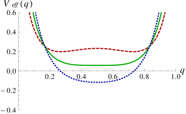
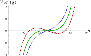
This effective potential exhibits a second-order phase transition, see Fig. 1. $V_{eff}(q)$ has the shape of a double-well potential symmetric to the confined vacuum $q_{c}=1/2.$ Depending on the value of $a,$ one can describe the transition from deconfinement to confinement:  At $a=0,$ the minima of the effective potential are given by the perturbative vacua at $q=0$ and $q=1.$ This is the region of complete QGP. For $0<a<a_{d}$ the system is in the semi-QGP phase, and the distance between the confined vacuum and the two degenerate minima starts decreasing. At $a_{d}=0.070230$ the transition to confinement takes place, and for $a\geqq a_{d}$ there is just one minimum which is given by the confined vacuum at $q=1/2$.

Figure 1: The effective potential, $V_{eff}(q)$ (left panel), and its first derivative, $V\prime_{eff}(q)$ (right panel), as a function of $q$. We present the plots for three different values of $a:$ $a<a_{d}$ (dashed) represents the semi-QGP, at $a=a_{d}$ (solid) the phase transition to confinement takes place, and for $a>a_{d}$ (dotted) the system is in the confined phase.

Figure 2: Left panel: the minimum of the effective potential as a function of $a,$ $q_{min}(a),$ using the linear term (solid), and the Vandermonde term (dashed). Right panel: the potential at the minimum as a function of $a,$ $V_{min}(a)$. Our fits to $q_{min}(a)$ and $V_{min}(a)$ are essentially identical to the exact numerical solutions, since we work with a high precision.

IV.1.1 Fixing the parameter at $T_{d}$

Apart from $T_{d}$, the effective potential of Eq. (41) involves three parameters $C_{1},\,C_{2},\,C_{3}$ which are determined from the lattice measurements of the pressure in the deconfined phase. First, we impose that the transition occurs at $T_{d}$. This implies that $a(T_{d})=a_{d}$ $:$

$$a_{d}=\frac{C_{1}}{1-C_{2}}\text{ ,}$$ (43)

which gives $C_{2}$ as a function of $C_{1}$. We further require that the pressure is zero at $T_{d}$ , which allows to determine $C_{3}$

$$\text{ }C_{3}=1-\frac{C_{1}\left[\text{L}\left(0.5\right)-a_{d}\text{ }8\pi^{2}\ln 2\right]}{3\frac{\zeta\left(3\right)}{2\pi}a_{d}}\text{ .}$$ (44)

Due to the two conditions, there is only one free parameter left, say $C_{1}$. This single parameter is utilized to fit the lattice pressure and the interaction measure.

IV.1.2 The minimum of the effective potential

The main numerical problem to compute the pressure $p(T)$ resides in finding the minimum of the effective potential as a function of $q$ at $T\geq T_{d}$. This defines a function $q_{min}(T)$.

For mathematical clarity, it is convenient to denote the $q$-dependent part of the effective potential in Eq. (41) as $V(q,a),$

$$V(q,a)=\text{L}\left(q\right)-2\pi\left[2\ln 2-\pi^{2}\left(q-\frac{1}{2}\right)^{2}\right]a(T)\ .$$ (45)

The minimum is found by solving numerically the equation

$${\frac{\partial V(q,a)}{\partial q}\mid}_{q=q_{min}}=0\ ,$$ (46)

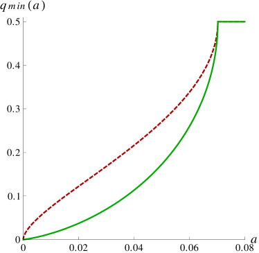
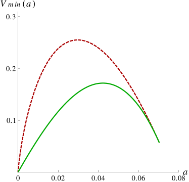
for different values of $a,$ in the range $0\leq a\leq a_{d}.$ This gives the minimum of the effective potential as a function $a,$ $q_{min}(a).$ We use this solution to obtain an expression for the potential at the minimum, which depends only on $a$

$$V_{min}(a)=V\left[q_{min}(a),a\right]\text{ .}$$ (47)

In principle, one needs to solve Eq. (46) for every value $0\leq a\leq a_{d}$ we want to study. However, it is more convenient to find a good ansatz for $q_{min}(a)$ and for $V_{min}(a)$. Then, it is straightforward to determine the temperature-dependent minimum by utilizing the definition for $a(T)$ in Eq. (42)

$$q_{min}(T) =q_{min}\left[a\left(T\right)\right]=q_{min}\left[\frac{\frac{T_{d}}{T}C_{1}}{\left(1-\frac{T_{d}}{T}C_{2}\right)}\right]\ ,$$

$$V_{min}(T) =V_{min}\left[a\left(T\right)\right]=V_{min}\left[\frac{\frac{T_{d}}{T}C_{1}}{\left(1-\frac{T_{d}}{T}C_{2}\right)}\right]\ .$$ (48)

To solve Eq. (46) we apply the numerical bisection method. Then we fit the numerical solutions for $q_{min}(a)$ and $V_{min}(a)$ with high precision. As an ansatz for the fits we use simple linear expansion in rational powers of $a,$ and in powers of $a_{d}-a$. The absolute deviation between the numerical solution and our ansatz for $V_{min}(a)$ is of the order of $10^{-7}$. It is important to work with good accuracy, because the error bars of the lattice data for the pressure $p/(3T^{3})$ are small, $10^{-5}$. In Fig. (2), we plot the solutions for $q_{min}(a)$ and for $V_{min}(a).$ Since we use a very high precision, the curves of our Ansätze coincide with the curves of the exact numerical solutions.

IV.1.3 Analytical expressions for the pressure and for the interaction measure

The pressure as a function of $T$ is obtained by plugging the solution $q_{min}\left(T\right)$ of Eq. (48) into the equation for the effective potential of Eq. (41)

$${\frac{p}{3T^{3}}}=\left(1-\frac{T_{d}}{T}C_{3}\right)\frac{\zeta\left(3\right)}{2\pi}+\frac{2\pi T_{d}}{3T}C_{1}\left\{2\ln 2-\pi^{2}\left[q_{min}(T)-\frac{1}{2}\right]^{2}\right\}\text{ }$$ (49)

$$\ +\frac{\left(1-\frac{T_{d}}{T}C_{2}\right)}{6\pi}\left\{\text{Li}_{3}\left[e^{i2\pi q_{min}(T)}\right]+\text{Li}_{3}\left[e^{-i2\pi q_{min}(T)}\right]-2\zeta\left(3\right)\right\}\text{ .}$$

Another possibility to compute the pressure is to directly use the ansatz for $V_{min}(T)$ depicted in Fig. (2) and in Eq. (48),

$${\frac{p}{3T^{3}}}=\left(1-\frac{T_{d}}{T}C_{3}\right)\frac{\zeta\left(3\right)}{2\pi}-\left(1-\frac{T_{d}}{T}C_{2}\right){\frac{\ V_{min}(T)}{3}}\text{ },$$ (50)

which greatly simplifies the numerics.

Differentiating the pressure of Eq. (49) with respect to $T,$ gives the interaction measure

$${\frac{\Delta}{3T^{3}}}=T{\frac{d}{dT}}\left(\frac{p}{3T^{3}}\right)\ .$$ (51)

Figure 3: Lattice data, as well as the numerical fits to the pressure $p/3T^{3}$ using the linear term. We present the curves in the one-parameter model (dashed), the two-parameter model (solid), and in the four-parameter fit (dotted). The horizontal lines represents the perturbative constant $c,$ which corresponds to the perturbative limit of the pressure. In the one- and in the two-parameter models $c=\zeta\left(3\right)/2\pi$ (solid), and in the four-parameter fit it is shifted by $\sim 0.5\%.$

Figure 4: Lattice data for the interaction measure $\Delta/3T^{3}$ in comparison with the results for the linear term. We present the curves in the one-parameter model (dashed), the two-parameter model (solid), and in the four-parameter fit (dotted).

Figure 5: Numerical fits to the lattice pressure $p/3T^{3}$ using the Vandermonde term $\sim T^{2}$. We show the curves in the one-parameter model (dashed), the two-parameter model (solid), and in the four-parameter fit (dotted). The horizontal lines represents the pressure in the perturbative limit.

Figure 6: Lattice interaction measure in comparison with the results for the Vandermonde term $\sim T^{2}$. We show the curves in the one-parameter model (dashed), the two-arameter model (solid), and in the four-parameter fit (dotted).

Notice, since $q_{min}(T)$ vanishes in the large-$T$ limit,

$$\lim_{T\rightarrow\infty}{\frac{p}{3T^{3}}}\rightarrow\frac{\zeta\left(3\right)}{2\pi}\ =c.$$ (52)

The constant $c$ is the solution to the pressure in the perturbative limit. At the same time, ${\frac{\Delta}{3T^{3}}}$ vanishes at large $T$.

Equations (49) and (51) are the final analytical results which are used to fit the lattice QCD data by adjusting the parameters of the model.

IV.2 Vandermonde potential

Utilizing the Vandermonde term of Eq. (35), the effective potential is given by

$$V_{eff} =V_{pt}+V_{npt}^{B}$$

$$=-3\frac{\zeta\left(3\right)}{2\pi}T^{3}\left(1-\frac{T_{d}}{T}C_{3}\right)$$

$$+T^{3}\left(1-\frac{T_{d}}{T}C_{2}\right)\left\{\text{L}\left(q\right)-4\pi\ln\left[2\sin(\pi q)\right]a(T)\right\}\text{ ,}$$ (53)

where $V_{npt}^{B}$ is the nonperturbative contribution constructed in Eq. (37). Repeating the analysis of Sec. IV.1 one can determine the minimum of the effective potential, $q_{min}(a),$ where the definition of the function $a(T)$ is now extended with a more general exponent,

$$a=\frac{\left(\frac{T_{d}}{T}\right)^{\delta}C_{1}}{\left(1-\frac{T_{d}}{T}C_{2}\right)}\text{ , \ }\delta=1,2\text{ }.$$ (54)

The $q_{min}(a)$ we obtain for the Vandermonde potential, again with a great accuracy, is depicted in Fig. (2). At $a=a_{d}$ the linear potential and the Vandermonde potential produce the same $V_{min}$ and $q_{min}.$

V Results

In this section we present the numerical results for the one- and the two-parameter matrix model, and compare them to the lattice data of Ref. Caselle et al. (2011b). We show the plots for the pressure, the interaction measure, and for the Polyakov loop utilizing three different options for the $q$-dependent nonperturbative term $\sim C_{1}$:  the linear term, $T^{2}T_{d}2\pi\left[2\ln 2-\pi^{2}(q-\frac{1}{2})^{2}\right]$, and the Vandermonde term $T^{3-\delta}\,{T_{d}}^{\delta}4\pi\log\left[2\sin(\pi q)\right]$, where we consider two different temperature dependences $\delta=1,2.$

Close to the critical temperature the lattice data become smeared out due to glueballs below $T_{d}$, the gluon mass above $T_{d}$, and lattice artifacts such as finite-volume effects. Therefore, it is convenient to apply a cut, and only fit the data at $T>1.05T_{d}$. Moreover the finite-volume effect also affects the pressure at high temperatures Panero (2008); Gliozzi (2007). In general, one finds that the pressure decreases with increasing volume. Motivated by the uncertainties on the lattice near $T_{d}$ and at high temperatures, we also discuss the possibility of introducing a four-parameter fit, and show the corresponding plots.

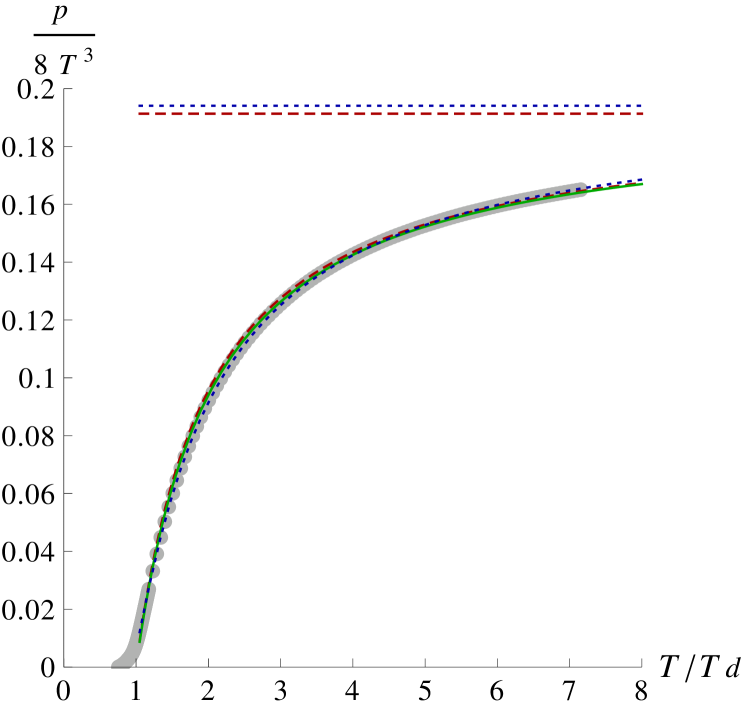
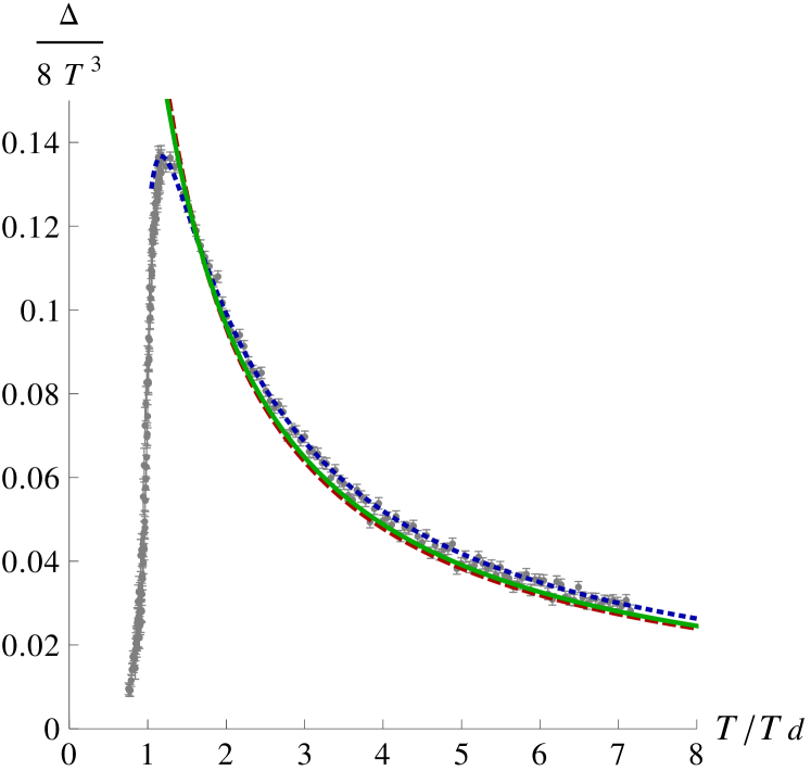
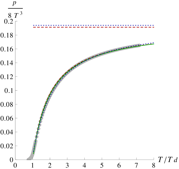
We determine the free parameters of the models by applying the corresponding nonlinear fits to the lattice pressure. First, we present the results for the pressure and for the interaction measure utilizing the linear term, Figs. (3) and (4), and the Vandermonde term, Figs. (5) and (6). For the Vandermonde term we just show the plots for the term $\sim T^{2}$, which provides in general better fits than the other temperature dependence $\sim T$. To give a better overview of the results we list the values of all parameters in Table (1). In this table we also include the results of the $\chi^{2}/\mathrm{d.o.f.}$ test to quantify how good our fit are. The lattice pressure has small error bars, $\sim 10^{-5}$. Therefore it is crucial that we achieve a high accuracy for our ansatz for $V_{min}(a),$ ${\sim 10^{-7},}$ to compare the best fits of the different models.

Non-pert. $V$	$C_{1}$	$C_{2}$	$C_{3}$	$\delta C_{3}$	$T_{d}$ rescale	$c$ rescale	$\chi^{2}$/dof
1 par. vdm1	0.000041	0.999408	0.999940	0	1	1	265.668
2 par. vdm1	0.000000	1.000000	1.000000	0.024311	1	1	202.275
4 par. vdm1	0.003657	0.947923	0.994911	0.010874	0.918032	1.031652	10.8481
1 par. vdm2	0.000030	0.999563	0.999956	0	1	1	285.664
2 par. vdm2	0.000000	0.999998	1.000000	0.025252	1	1	207.833
4 par. vdm2	0.006322	0.909976	0.990921	0.103102	0.855040	0.999717	1.09882
1 par. vlin	0.000035	0.999489	0.999948	0	1	1	258.051
2 par. vlin	0.000001	0.999981	0.999998	0.023831	1	1	199.179
4 par. vlin	0.033310	0.525695	0.952861	-0.16002	0.907484	1.014434	0.54232

Table 1: Parameters which give the best fits to the lattice pressure for different nonperturbative terms. We use the following notation: “1 par.” for the one-parameter model, “2 par.” for the two-parameter model, and “4 par.” for the four-parameter fit. Moreover, “vlin” denotes the linear term, “vdm1” the Vandermonde term $\sim T,$ and “vdm2” the Vandermonde term $\sim T^{2}.$ The parameters $C_{2}$ and $C_{3}$ are not free, they are a function of $C_{1}$. In “1 par.” we utilize $C_{1}$ as the single free parameter to fit the lattice data. In “2 par.” we add a second free parameter $\delta C_{3}=C_{3}(T_{d})-C_{3}(\infty)$, defined in Eq. (55), to include the effects of the bag model constant $B$. In “4 par.” we further allow for small shifts in $T_{d},$ and in the perturbative constant $c,$ in order to encompass other possible nonperturbative effects not included in our matrix model. Moreover, we also show the results of the $\chi^{2}/dof$ test for our fits to the lattice pressure.

V.1 Results of the one-parameter model

The one-parameter model exhibits only mild sensitivity to the choice of the $q$-dependent nonconstant terms. By adjusting the only free parameter of the model we already obtain good agreement with the lattice pressure and with the interaction measure. Especially at high and low temperatures the fits are close to the lattice data. At intermediate temperatures the agreement becomes slightly worse. Moreover, the one-parameter model fails to reproduce the correct shape of the peak in the interaction measure, residing at $T\sim 1.14T_{d}$.

An important observation is that in the one-parameter model the best fit to the lattice pressure gives always a rather small value of $C_{1}$, see Table 1. From Eq. (48) and Fig. (2) one can deduce that the smaller the value for $C_{1},$ the faster the condensate for $q$ approaches zero above the critical temperature. If $q_{min}(T)\approx 0$ all $q$-dependent terms in the effective potential vanish. This implies that, except from a narrow region close to $T_{d},$ the thermodynamics is completely governed by the $q$-independent ideal term $\sim T^{3}$ plus the constant term $\sim T^{2}T_{d}$.

V.2 Two-parameter model

Aiming to improve the results of the one-parameter model, we consider the two-parameter model, as proposed in Ref. Dumitru et al. (2012). In the two-parameter model the constants $C_{1}$ and $C_{2}$ remain the same as before, but $C_{3}$ is replaced by the temperature-dependent parameter

$$C_{3}(T)=C_{3}\left(\infty\right)+\frac{C_{3}\left(T_{d}\right)-C_{3}\left(\infty\right)}{T^{2}/T_{d}^{2}}\text{ ,}$$ (55)

which is equivalent to adding an MIT bag constant $B$.

We find again that the results are quite similar for the linear term and the Vandermonde term. The two-parameter fit improves the results of the one-parameter model at intermediate temperatures, and gives overall good agreement with the lattice data in the entire temperature region, see Figs. (3) and (4). Only at the peak of the interaction measure do our results deviate notably from the lattice results. It must be pointed out, however, that the parameters of the model are fixed by imposing that the pressure vanishes at the transition point. Instead, it would be necessary to fit the pressure in the confined phase to some hadronic (glueball) resonance gas. Therefore, one should not expect to fit the lattice data close to $T_{d}$ with a great accuracy by making this simple assumption.

Moreover, the two-parameter model also produces an extremely narrow region in which the condensate for $q$ is nonvanishing.

V.3 Four-parameter fit

The one- and the two-parameter models give already good fits to the lattice pressure and to the interaction measure. However, at the peak of the interaction measure, residing close to $T_{d}$, the agreement becomes notably worse. Further, due to the small error bars of the lattice pressure, the $\chi^{2}/dof$ test still gives a large value $\sim$ ${200.}$

Therefore it is interesting to investigate, wether further extending the number of degrees of freedom can improve the results near the critical temperature, and reproduce the correct shape for the interaction measure peak. In this work, the possibility of introducing a four-parameter fit is discussed, which can be motivated in two ways. First, in our analytical calculations we make two obvious approximations:  We compute the perturbative potential only to one-loop order, and we impose that the pressure must vanish at the transition point. Moreover, due to the smearing and finite-volume effects present on the lattice close to $T_{d}$ and in the high-temperature region, it is difficult to determine the exact values for the critical temperature, and for the pressure in the perturbative limit. Taking these uncertainties into account, two additional free parameters are introduced in the two-parameter matrix model, one for $T_{d},$ and one for $c$, which corresponds to the perturbative limit of the pressure, see Eq. (52). We note that this four-parameter fit should be regarded just as an approximation to a more complete model including an effective theory for the confined phase.

The two additional parameters provide a perfect agreement with the lattice pressure and with the interaction measure for all the three nonconstant terms considered in this work, see Figs. (3), (4), (5), and (6). Especially close to $T_{d}$ the results improve notably, giving a good fit to the peak of the interaction measure, with $\chi^{2}/\mathrm{d.o.f.}\sim 0.5$ for the model with a linear term. This shows that the difference between the model and the lattice pressure is smaller than the error bars.

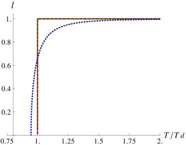
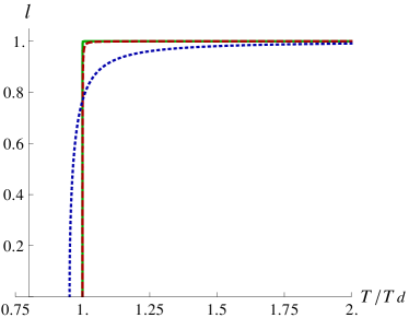
An important result is that the four-parameter fit gives a significantly larger value of $C_{1}$ than the other two models, see Table (1). This implies that there is a transition region in the deconfined phase, in which the system develops a non-trivial condensate for $q$, $\ q_{min}(T)\neq 0$. In our matrix model this happens in principle at all temperatures. But in practice, the condensate is only numerically large below $\sim 1.2\,T_{d}$ for the linear and for the Vandermonde term, which will become clear when we discuss the Polyakov loop, Fig. (8). This is the range where the details of the matrix model are relevant, since the $q$-dependent terms of the effective theory provide a nontrivial contribution in the deconfined phase. Notably, this is in accordance with the results in $d=3+1$, where the condensate is nonzero up to $\sim 1.2T_{d}.$

In Table (1) we list the values for the parameters. The deviation in $c$ is rather small for all nonconstant terms, and can be explained as follows. At high tmperature the lattice pressure is slightly volume-dependent, and tends to decrease with increasing volume, see Ref. Panero (2008); Gliozzi (2007). This implies that on the lattice the value of $c$ may be shifted to lower values when the volume is increased. Moreover, this small shift in $c$ could be partly due to the applied one-loop approximation. Extending the calculation to higher-loop order will shift the perturbative constant. Thus, the higher-order loop calculations and the volume dependence could account for the difference in $c$.

In what concerns the shift in $T_{d},$ we note that the lattice results for the interaction measure show that there is a significant energy density below $T_{d}$. This arises from two effects. One is simply an uncertainty of the transition temperature, which is affected by finite-size effects such as critical slowing down. For $N=2$ the transition is of second order. Further, from Eq. (1), in three dimensions the ratio of $T_{d}/\sqrt{\sigma}$ is higher than it is in $d=3+1$, remember $\sigma$ is the string tension. If the ratio of the glueball masses to $\sqrt{\sigma}$ is approximately independent of the dimensionality, then the contribution of a glueball gas to the energy density may be more significant near $T_{d}$ in three dimensions than in four. Such effects from the confined phase are completely neglected in our model. Ideally, we should develop an effective theory for the confined phase, and match that to the matrix model in the deconfined phase. Failing to do that, we adopt the prescription of the four-parameter fit, which we admit is an approximation to a more complete theory.

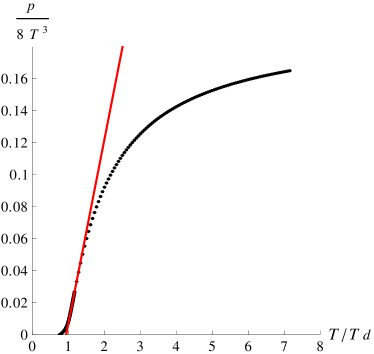
We then define the transition temperature as the point where a linear fit to the pressure intercepts the $T$-axis. In this case, the best estimate of $T_{d}$ is obtained by the intercept of the tangent to the inflection point with the $T$-axis. The inflection point is the point where the derivative is maximum, and the second derivative vanishes. As shown in Fig. (7), the intercept occurs at $0.94\,T_{d}$. This value is closer to results for the rescaled critical temperature in the four-parameter fit, see Table (1).

Summing up, considering the possible systematic errors, the four-parameter fit allows us to obtain good agreement with the lattice results in the entire temperature range $T_{d}\leq T\leq 8T_{d}$, and well reproduces the peak of the conformal anomaly.

Figure 7: We define $T_{d}$ by interpolating the tangent to the inflection point of the pressure, which occurs at $T=1.14T_{d}$. The point where the tangent hits the $T$-axis defines the transition temperature: $T_{d}^{\ast}\equiv 0.94.$

V.4 Polyakov loop

Utilizing the parameters listed in Table (1), which are determined by fitting the lattice data for the pressure, it is possible to compute the Polyakov loop from Eq. (7). Figs. (8) and (9) show the Polyakov loop for the linear term and for the Vandermonde term $\sim T^{2}$ using the one- and the two-parameter model, as well as the four-parameter fit. In the one- and in the two-parameter model, the Polyakov loop grows sharply from $0$ to $1$ above the critical temperature. To understand this behavior we remember that the Polyakov loop is given by $l\mathbf{=}\cos\left[\pi q_{min}(T)\right].$ Thus, $l$ is only then not equal to one in the deconfined phase, if the minimum of the effective potential differs from zero. In the one- and two-parameter model however, the condensate, $q_{min}(T),$ is only numerically large in a narrow range close to $T_{d},$ and then it effectively vanishes. This implies that the system merges rapidly from confinement, $q=0,$ into the perturbative vacuum, $q=1.$

In the four-parameter fit, which perfectly agrees with the lattice pressure, the condensate is non-vanishing up to $\sim 1.2T_{d}$ for both nonperturbative terms. Therefore the Polyakov loop markedly varies from one in this temperature region. Notably, the width of the transition range is widely independent of the details of the nonconstant terms discussed in this work.

Figure 8: Left panel: the Polyakov loop obtained using the linear term, in the one-parameter model (dashed), the two-parameter model (solid), and in the four-parameter fit (dotted). Right panel: the ’t Hooft loop divided by its perturbative limit, $\alpha_{0}^{pert}=5.104.$ The plots of the one- and of the two-parameter model coincide.

Figure 9: The Polyakov loop (left panel), and the ’t Hooft loop scaled by its perturbative value, $\alpha_{0}^{pert}=5.104$ (right panel). The plots are obtained utilizing the Vandermonde term $\sim T^{2},$ in the one-parameter model (dashed), the two-parameter model (solid), and in the four-parameter fit (dotted). For the one- and the two-parameter model the curves essentially coincide.

VI Interface tension

In this section we construct the interface tension for our model, and present the results for the ’t Hooft loop. In absence of dynamical quarks the $SU(N)$ gauge theories exhibit a global $Z(N)$ symmetry associated with the center of the gauge group. The confined vacuum is symmetric under $Z(N)$ transformations, whereas in the deconfined phase the $Z(N)$ symmetry is spontaneously broken. If the system is infinite, then the spontaneous symmetry breakdown is related to the occurrence of $N$ degenerate vacua. In a finite volume however, bubbles of different vacua can form, which are separated by domain walls. The dynamics of these bubbles is governed by the action of the domain walls, which is proportional to the interface tension.

The $Z(N)$ interface tension gives the tunneling probability between two different vacua of the system. Following the discussion of Refs. Korthals Altes et al. (1997); Dumitru et al. (2012), we construct the interface by putting the system in a long tube of length $2L$ in the $z$ direction, and of length $L_{t}$ in the other two spatial directions, with $L$ $\gg$ $L_{t}\gg$ $\beta,$ and $L\rightarrow\infty$. The volume in the directions transverse to $z$ is $\mathcal{V}_{tr}=\beta L_{t}$. To model the interface tension we assume that the system is in a vacuum state at both ends, but not in between. This forces a $Z(N)$ interface along the $z$-direction. The action of the interface is equal to the interface tension $\alpha$, times the transverse volume, $\mathcal{V}_{tr}$

$$\alpha=\frac{S}{\mathcal{V}_{tr}}\text{ .}$$ (56)

To compute the interface tension one first needs to construct the effective action $S,$ which is given by the effective potential plus a kinetic term

$$S=\mathcal{V}_{tr}\int dz\left[\mathcal{T}_{kin}(q)+V_{eff}(q)\right]\text{ .}$$ (57)

At leading order, for $q$ varying slowly on the scale of $1/T,$ it is sufficient to use the kinetic term at tree level, which is given by the classical action

$$\mathcal{T}_{kin}(q) =\frac{1}{2}\operatorname{tr}G_{\mu\nu}^{2}=\frac{\pi^{2}T^{2}}{g^{2}}\left(\frac{dq}{dz}\right)^{2}\operatorname{tr}\sigma_{3}^{2}$$ (58)

$$\equiv\frac{T^{3}}{2}\left(\frac{dq}{dz\prime}\right)^{2}\text{ ,}$$

where we introduce the rescaled coordinate $z$

$$\text{ }z\prime=\frac{z}{\gamma}\text{ , \ \ }\gamma=\frac{2\pi}{g\sqrt{T}}\text{ .}$$ (59)

$\gamma$ is the parameter which controls the width of the domain wall between the two vacua. Notice, at the classical level the action reduces to only a kinetic term, since the classical field of Eq. (4) commutes with itself. This means that classically there is no difference between the two vacua.

Assuming that the vacua at the two ends of the box, $z=-L$ and $z=+L$, correspond to the two minima, $q_{i}$ and $q_{f}$, the interface tension is connected to the shortest path between $q_{i}$ and $q_{f}$ , which obeys the equation of motion

$$T^{3}\frac{d^{2}q}{dz\prime^{2}}=\frac{dV_{eff}(q)}{dq}\text{ },$$ (60)

with the boundary conditions $q(-L)=q_{i}$ and $q(L)=q_{f}$. The corresponding energy density is obtained by multiplying Eq. (60) by $dq/dz\prime$, and integrating over $z\prime$

$$e=\frac{T^{3}}{2}\left(\frac{dq}{dz\prime}\right)^{2}-V_{eff}(q).$$ (61)

For any solution to the equation of motion the energy is conserved, $de/dz\prime=0$. Therefore,

any function $q(z)$ which minimizes the effective action with respect to the corresponding boundary conditions satisfies:

$$\text{ }\frac{T^{3}}{2}\left(\frac{dq}{dz\prime}\right)^{2}=V_{eff}(q)\text{ , \ \ \ }\frac{dq}{dz\prime}=\sqrt{\frac{2V_{eff}(q)}{T^{3}}}\text{ .}$$ (62)

Using the energy conservation in Eq. (62), the effective action can be written as

$$S =2\mathcal{V}_{tr}\int dzV_{eff}(q)$$

$$=\gamma\sqrt{T^{3}}\mathcal{V}_{tr}\int_{q_{i}}^{q_{f}}dq\sqrt{2V_{eff}(q)}$$

$$=\frac{2\pi}{g}T\mathcal{V}_{tr}\int_{q_{i}}^{q_{f}}dq\sqrt{2V_{eff}(q)\text{ }}\text{ .}$$ (63)

The general form for the interface tension is then

$$\alpha=\alpha_{0}\frac{\sqrt{T^{5}}}{g}\text{ , }$$ (64)

where we define the dimensionless quantity

$$\alpha_{0}=2\pi\int_{q_{i}}^{q_{f}}dq\sqrt{\frac{2V_{eff}(q)}{T^{3}}}\text{ }.$$ (65)

It is interesting to notice that the factor $1/g^{2}$ present at the classical level in Eq. (58), becomes $1/g.$ This is because the effective action acquires a potential only at one-loop order. Furthermore, from the definition of the rescaled length $z\prime$ in Eq. (59) follows that the relevant distance scale in the effective action is not $1/T$ , but $1/g\sqrt{T}$. Therefore, if the coupling constant is small, the effective action varies over much larger distance scales than $1/T$ . This implies that in weak coupling the variation of $q(z)$ in space is slow and can be ignored.

VI.1 The order-order interface tension

Above the deconfinement temperature the theory can be in one $Z(N)$ vacuum, $q_{i}=q_{min}^{1}(T),$ at one end of the box, and in a degenerate but inequivalent vacuum, $q_{f}=q_{min}^{2}(T),$ at the other end. Due to the $Z(2)$ symmetry $q_{min}^{2}(T)=1-q_{min}^{1}(T).$ This is the order-order interface tension, which is equivalent to a ’t Hooft loop in the deconfined phase. The associated tunneling probability is determined by the integral

$$\alpha_{0}=2\pi\int_{q_{min}^{1}(T)}^{q_{min}^{2}(T)}dq\sqrt{\frac{2V_{eff}(q)}{T^{3}}}\text{ ,}$$ (66)

where $V(q)$ is the difference between the effective potential in $q$ and at the minimum

$$V(q)=V_{eff}(q,T)-V_{eff}\left[q_{min}^{1}(T)\right]\text{ .}$$ (67)

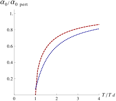
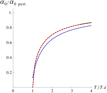
Figures 8 and 9 show the plots for the ’t Hooft loop scaled by its perturbative limit, $\alpha_{o}^{pert}=5.104.$ In the one-parameter model the results are essentially the same when using the linear term and the Vandermonde term. One can understand this by remembering that in the one-parameter model the minimum of the effective potential merges rapidly from the confined vacuum, $q_{min}(T_{d})=q_{c}=0.5$, into the perturbative vacuum, $q_{min}(T>T_{d})\approx 0.$ Therefore, the two degenerate minima are approximately at $q_{min}^{1}(T)\approx 0$ and $q_{min}^{2}(T)\approx 1.$ Remarkably, unlike the Polyakov loop, which becomes trivial in the one-parameter model, for the ’t Hooft loop the details of the matrix model are relevant in the entire semi-QGP for all models addressed in this work.

VII Conclusions and outlook

In this work we utilize a matrix model to study the deconfinement phase transition in pure $SU(2)$ glue theory in $2+1$ dimensions. The basic variables of the model are the eigenvalues of the Wilson line. First we construct the effective potential as the sum of a perturbative and a nonperturbative part. The perturbative potential is computed in the presence of a constant background field for the vector potential $A_{0}\sim q.$ We find that to one-loop order this gives a trilogarithm function of $A_{0}/T.$ Then, in order to model the transition to deconfinement, we introduce additional constant and nonconstant nonperturbative terms depending on $T,$ and on three parameters. For the nonconstant terms, which are functions of $q,$ we try three different Ansätze: the linear term $\sim T^{2}T_{d}2\pi\left[2\ln 2-\pi^{2}(q-\frac{1}{2})^{2}\right]$, and a Vandermonde-like term with two different temperature dependences, $\sim T^{3-\delta}\,{T_{d}}^{\delta}4\pi\log\left[2\sin(\pi q)\right],$ $\delta=1,2$. Imposing two constraints for the phase transition at $T=T_{d}$ leaves only one free parameter, which is determined by fitting the lattice pressure. The numerical results for the pressure and for the interaction measure are presented and compared to the lattice data of Ref. Caselle et al. (2011b).

The one-parameter model already gives good fits to the lattice pressure and to the interaction measure at high and low temperatures. But at intermediate temperatures the results deviate from the lattice results. The two-parameter model improves the agreement at intermediate temperatures, and provides overall good fits to the pressure, and to the interaction measure at all temperatures. However, in both models there is a clear deviation from the lattice data at the peak of the interaction measure, while their $\chi^{2}$/d.o.f. tests indicate that better fits are possible. Considering different options to cure this deficiency, the possibility of constructing a four-parameter fit is discussed. Regarding possible uncertainties present in our analytical calculations, due to the applied approximations, as well as on the lattice, due to glueballs and finite-volume effects, the two-parameter model is extended by two additional free parameters: one for $T_{d},$ and one for the perturbative limit of the pressure, $c.$ The four-parameter model gives remarkably good fits to the lattice pressure and to the interaction measure for all nonconstant terms discussed in this work. It also reproduces the correct shape for the peak of the conformal anomaly. Furthermore, in the four-parameter fit there is a range in the deconfined phase, where the condensate is nonzero, and the details of the matrix model become relevant. The window of this transition region extends up to $\sim 1.2$ $T_{d}.$ This is similar to the results for the $SU(2)$ matrix model obtained in $d=3+1$. We remark however, that this four-parameter fit should be considered just as a possible approximation to a more complete model which involves an underlying effective theory for the confined phase. Notably, the one- and the two-parameter model, as well the four-parameter fit exhibit only a mild sensitivity to the details of the nonconstant terms.

Using the parameters determined by fitting the pressure, we also show the plots for the Polyakov loop and for the ’t Hooft loop. In the one- and in the two-parameter model the Polyakov loop grows sharply from $0$ to $1$ above above the critical temperature. This is because in our model the Polyakov loop differs from one only when the condensate for $q$ is nonvanishing. In the one- and the two-parameter model, however, the condensate effectively vanishes rapidly above $T_{d}.$ In the four-parameter fit the transition range where the condensate is nonvanishing and where the Polyakov loop varies from one extends up to $\sim 1.2\;T_{d}.$

The model can be improved in two obvious ways. First, one can include perturbative corrections at next to leading order, to $\sim g^{2}$. This will presumably correct the deviation from the lattice data at high temperature. Second, near $T_{d}$ it is necessary to include an effective theory for the confined phase. This will describe the increase in the energy density near $T_{d}$, and obviate our rather ad hoc prescription for shifting $T_{d}$ by hand.

Summing up, the one- and the two-parameter matrix models work reasonably well for the pressure and for the interaction measure. They also provide reasonable predictions for the ’t Hooft loop. The four-parameter fit agrees perfectly with the lattice data even very close to $T_{d}$. Moreover, it provides reasonable results for the Polyakov loop. This is closely related to the width of the transition region, in which the model exhibits a nontrivial minimum. So far, the behavior of the Polyakov loop and of the ’t Hooft near $T_{d}$ in $d=2+1$ have not been computed on the lattice. These results could provide important tests of our model.