Correlations between charge radii, E0 transitions, and M1 strength

Abstract

In the framework of the interacting boson model, relations are derived between nuclear charge radii, electric monopole transition rates, and summed magnetic dipole transition in even-even nuclei. The proposed correlations are tested in the rare-earth region.

I Introduction

In recent papers Zerguine08 ; Zerguine12 a simultaneous description was proposed of charge radii and electric monopole transitions of nuclei in the rare-earth region. The purpose of the studies was to examine to what extent a purely collective interpretation of nuclear $0^{+}$ levels is capable of yielding a coherent and consistent picture of both properties.

In this contribution a further correlation is proposed between both of the above properties and summed M1 strength as observed in even-even nuclei. The framework used to establish this correlation is the interacting boson model (IBM) of Arima and Iachello Iachello87 which describes nuclear collective excitations in terms of $s$ and $d$ bosons with angular momenta $\ell=0$ and 2, respectively. The simplest version of the model is used, IBM-1, which makes no distinction between neutron and proton bosons.

A brief recall of the necessary operators is given in Sect. II and previous results Zerguine12 on isotope shifts are summarized in Sect. III. Correlations between the summed M1 strength and isotope shifts, isomer shifts, and $\rho({\rm E0})$ values are pointed out in Sects. IV, V, and VI, respectively. Finally, topics for further study are listed in Sect. VII.

II Operators in the IBM-1

In the IBM-1 the charge radius operator is taken as the most general scalar expression, linear in the generators of U(6) Iachello87 ,

$$\hat{T}(r^{2})=\langle r^{2}\rangle_{\rm c}+\alpha N_{\rm b}+\eta\frac{\hat{n}_{d}}{N_{\rm b}},$$ (1)

where $N_{\rm b}$ is the total number of $s$ and $d$ bosons, $\hat{n}_{d}$ is the $d$-boson number operator, and $\alpha$ and $\eta$ are coefficients with units of length². The first term in Eq. (1), $\langle r^{2}\rangle_{\rm c}$, is the square of the charge radius of the core nucleus. The second term accounts for the (locally linear) increase in the charge radius due to the addition of two nucleons. The third term in Eq. (1) stands for the contribution to the charge radius due to deformation. It is identical to the one given in Ref. Iachello87 but for the factor $1/N_{\rm b}$. This factor is included here because it is the fraction $\langle\hat{n}_{d}\rangle/N_{\rm b}$ which is a measure of the quadrupole deformation ($\beta^{2}$ in the geometric collective model) rather than the matrix element $\langle\hat{n}_{d}\rangle$ itself.

Two quantities can be derived from charge radii: isotope and isomer shifts. The former measures the difference in charge radius of neighboring isotopes. For the difference between even-even isotopes one finds from Eq. (1)

$$\Delta\langle r^{2}\rangle \equiv \langle r^{2}\rangle_{0_{1}^{+}}^{A+2}-\langle r^{2}\rangle_{0_{1}^{+}}^{A}$$ (2)

$$= |\alpha|+\frac{\eta}{N_{\rm b}}\left(\langle\hat{n}_{d}\rangle^{A+2}_{0_{1}^{+}}-\langle\hat{n}_{d}\rangle^{A}_{0_{1}^{+}}\right),$$

where $\langle\hat{n}_{d}\rangle_{J^{\pi}}$ is a short-hand notation for $\langle J^{\pi}|\hat{n}_{d}|J^{\pi}\rangle$. Isomer shifts are a measure of the difference in charge radius between an excited (e.g., the $2_{1}^{+}$) state and the ground state, and are given by

$$\delta\langle r^{2}\rangle \equiv \langle r^{2}\rangle^{A}_{2_{1}^{+}}-\langle r^{2}\rangle^{A}_{0_{1}^{+}}$$ (3)

$$= \frac{\eta}{N_{\rm b}}\left(\langle\hat{n}_{d}\rangle^{A+2}_{2_{1}^{+}}-\langle\hat{n}_{d}\rangle^{A}_{2_{1}^{+}}\right).$$

Once the form of the charge radius operator is determined, the E0 transition operator follows from the relation Zerguine08 ; Zerguine12

$$\hat{T}({\rm E0})=(e_{\rm n}N+e_{\rm p}Z)\hat{T}(r^{2}),$$ (4)

where $e_{\rm n}$ ($e_{\rm p}$) is the neutron (proton) effective charge. Since for E0 transitions the initial and final states are different, neither the constant $\langle r^{2}\rangle_{\rm c}$ nor $\alpha N_{\rm b}$ in Eq. (1) contribute to the transition, and the $\rho({\rm E0})$ value equals

$$\rho({\rm E0};i\rightarrow f)=\frac{e_{\rm n}N+e_{\rm p}Z}{eR^{2}}\frac{\eta}{N_{\rm b}}|\langle f|\hat{n}_{d}|i\rangle|.$$ (5)

The magnetic dipole operator in the IBM-1 is of the form Iachello87

$$\hat{T}({\rm M1})=\sqrt{\frac{3}{4\pi}}\left(g_{\nu}\hat{L}_{\nu}+g_{\pi}\hat{L}_{\pi}\right),$$ (6)

where $\hat{L}_{\nu}$ ($\hat{L}_{\pi}$) is the angular momentum operator for the neutrons (protons) and $g_{\nu}$ ($g_{\pi}$) the $g$ factor of the neutron (proton) boson.

III Isotope shifts

To test the relation between charge radii and E0 transitions, a systematic study of even-even isotopes from Ce ($Z=58$) to W ($Z=74$) was carried out in Ref. Zerguine12 . The analysis required the knowledge of structural information concerning the ground and excited levels to which an IBM-1 Hamiltonian is adjusted. A general one- and two-body Hamiltonian is taken with six parameters which are constant for a given isotope series, except one which is allowed to vary with valence neutron and proton numbers. Details can be found in Ref. Zerguine12 .

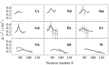
Figure 1: Experimental (points) and calculated (lines) isotope shifts $\Delta\langle r^{2}\rangle$, for isotopic chains in the rare-earth region from Ce to W. The data are taken from Ref. Cheal03 for Ce, from Ref. Otten89 for Nd, Sm, Dy, Er, and Yb, from Ref. Fricke95 for Gd, from Ref. Angeli04 for Hf, and from Ref. Jin94 for W.

Once the IBM-1 Hamiltonian is obtained for a given nucleus, matrix elements of the operators discussed in Sect. II depend solely on the coefficients appearing in the operators. Isotope shifts $\Delta\langle r^{2}\rangle$, according to Eq. (2), depend on the coefficients $|\alpha|$ and $\eta$. The coefficient $|\alpha|$ is adjusted for each isotope series separately, while $\eta$ is kept constant for all isotopes, $\eta=0.50$ fm². The resulting isotope shifts are shown in Fig. 1. The largest peaks in the isotope shifts occur for ^152-150Sm, ^154-152Gd, and ^156-154Dy, that is, for the difference in radii between $N=90$ and $N=88$ isotopes. The peak is smaller below $Z=62$ for Ce and Nd, and fades away above $Z=66$ for Er, Yb, Hf, and W.

IV Correlation between M1 strength and isotope shifts

It is known from the work of Ginocchio Ginocchio91 that the summed M1 strength from the ground state to the scissors mode (for a review on the latter, see Ref. Heyde10 ) is related to the ground-state matrix element of the $d$-boson number operator $\hat{n}_{d}$,

$$S({\rm M1};0^{+}_{1}) \equiv \sum_{f}B({\rm M1};0^{+}_{1}\rightarrow 1^{+}_{f})$$ (7)

$$= \frac{3}{4\pi}(g_{\nu}-g_{\pi})^{2}\frac{6N_{\nu}N_{\pi}}{N_{\rm b}(N_{\rm b}-1)}\langle\hat{n}_{d}\rangle_{0^{+}_{1}},$$

where $N_{\nu}$ ($N_{\pi}$) is the number of neutron (proton) bosons and the sum is over all possible $1^{+}$ states characterized by the label $f$.

To establish a connection between summed M1 strength and isotope shifts, one rewrites the relation (7) as follows:

$$\tilde{S}({\rm M1};0^{+}_{1}) \equiv \frac{N_{\rm b}-1}{N_{\nu}}S({\rm M1};0^{+}_{1})$$ (8)

$$= \frac{9}{2\pi}(g_{\nu}-g_{\pi})^{2}\frac{N_{\pi}}{N_{\rm b}}\langle\hat{n}_{d}\rangle_{0^{+}_{1}}.$$

The rewritten relation is such that all $N$-dependent quantities (i.e., $N_{\rm b}$ and $N_{\nu}$) are shifted to the left-hand side of the equation, except for the factor $1/N_{\rm b}$ which precisely coincides with the $N$ dependence as it appears in the definition of the isotope shifts (2). The tilde in $\tilde{S}({\rm M1};0^{+}_{1})$ is used as a reminder that it is not the summed M1 strength but rather the summed M1 strength weighted by an $N$-dependent factor. One now defines the difference

$$\Delta\tilde{S}({\rm M1})\equiv\tilde{S}({\rm M1};0^{+}_{1})^{A+2}-\tilde{S}({\rm M1};0^{+}_{1})^{A}$$ (9)

$$=\frac{9}{2\pi}(g_{\nu}-g_{\pi})^{2}\frac{N_{\pi}}{N_{\rm b}}\left(\langle\hat{n}_{d}\rangle^{A+2}_{0_{1}^{+}}-\langle\hat{n}_{d}\rangle^{A}_{0_{1}^{+}}\right).$$

The quantity between brackets on the right-hand side of Eq. (9) is precisely the one that occurs in the expression (2) for the isotope shift and hence the following relation is established:

$$\Delta\tilde{S}({\rm M1})=\frac{9}{2\pi}\frac{(g_{\nu}-g_{\pi})^{2}}{\eta}N_{\pi}\left(\Delta\langle r^{2}\rangle-|\alpha|\right).$$ (10)

This relation is different from the one proposed by Heyde et al. Heyde93 which correlates summed M1 strength and charge radii themselves. This has two drawbacks: (i) the quantity $\langle r^{2}\rangle_{\rm c}$, which appears in the operator (1), is ill determined and (ii) charge radii are not that well known as their differences (isotope shifts). The relation (10) is model dependent since it involves the coefficient $\alpha$ which cannot be neglected (it represents an important part of the isotope shift) and which varies from one isotope series to another. Nevertheless, with the values for $\alpha$ obtained from the isotope shifts (see Sect. III), the relation (10) can be tested in the rare-earth region. The slope in the correlation plot depends on the constants $\eta$ and $g_{\nu}-g_{\pi}$. The former is known from the isotope shifts while the latter can be obtained by adjusting the expression (7) to the observed summed M1 strength in rare-earth nuclei Pietralla95 ; Enders05 , leading to $|g_{\nu}-g_{\pi}|\approx 0.83$ $\mu_{\rm N}$.

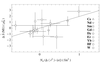
Figure 2: Test of the relation (10) between differences of summed M1 strength in neighboring isotopes and isotope shifts. The summed M1 strength is taken from Ref. Enders05 . The slope of the line is determined by $\eta$ and $g_{\nu}-g_{\pi}$, coefficients that appear in the charge radius and M1 operators, respectively.

The resulting correlation plot is shown in Fig. 2. Two compilations exist of the observed summed M1 strength, one by Pietralla et al. Pietralla95 and a second by Enders et al. Enders05 . They give broadly consistent results and hence lead to similar correlation plots. The latter, more recent compilation is taken here. Large error bars on both quantities preclude at the moment a conclusive test of the proposed correlation. In addition, there is an uncertainty (not included in Fig. 2) associated with the coefficient $\alpha$. The large errors follow from poorly determined isotope shifts (e.g., in dysprosium) but also because differences of summed M1 strength should be considered and not the summed M1 strength itself.

An alternative strategy, to be explored in the future, is to use the relation (10) to fix the coefficients $\alpha$ from the experimental summed M1 strength and use the resulting values in the calculation of nuclear radii.

V Correlation between M1 strength and isomer shifts

The relation (7) has been generalized to summed M1 strength from an arbitrary state to the scissors mode built on top of that state Ginocchio97 ; Smirnova02 ,

$$S({\rm M1};J_{i})\equiv\sum_{f(\neq i)}B({\rm M1};J_{i}\rightarrow J_{f})=\frac{3}{4\pi}(g_{\nu}-g_{\pi})^{2}\frac{6N_{\nu}N_{\pi}}{N_{\rm b}(N_{\rm b}-1)}\left(\langle\hat{n}_{d}\rangle_{J_{i}}-\frac{J_{i}(J_{i}+1)}{6N_{\rm b}}\right),$$ (11)

where the initial state $i$ is excluded from the sum over $f$. The difference

$$\delta S({\rm M1})\equiv S({\rm M1};2^{+}_{1})-S({\rm M1};0^{+}_{1})=\frac{3}{4\pi}(g_{\nu}-g_{\pi})^{2}\frac{6N_{\nu}N_{\pi}}{N_{\rm b}(N_{\rm b}-1)}\left(\langle\hat{n}_{d}\rangle_{2_{1}^{+}}-\frac{1}{N_{\rm b}}-\langle\hat{n}_{d}\rangle_{0_{1}^{+}}\right),$$ (12)

contains the same combination of matrix elements of $\hat{n}_{d}$ as the one that appears in the isomer shift (3), and therefore the following relation is established:

$$\delta S({\rm M1})=\frac{9}{2\pi}\frac{(g_{\nu}-g_{\pi})^{2}}{\eta}\frac{N_{\nu}N_{\pi}}{N_{\rm b}-1}\left(\delta\langle r^{2}\rangle-\frac{\eta}{N_{\rm b}^{2}}\right).$$ (13)

Some isomer shifts are known in the rare-earth region; the data are more than 30 years old and often discrepant. Nothing is known about M1 strength built on excited states. The relation (13) therefore remains untested.

VI Correlation between M1 strength and $\rho$(E0) values

The E0 operator is directly proportional to $\hat{n}_{d}$, unlike the charge radius operator which involves additional terms which complicate the relation between the summed M1 strength and charge radii, as shown above. On the other hand, the matrix element of $\hat{n}_{d}$ appearing in the sum rule (7) is diagonal while a $\rho({\rm E0})$ value involves a non-diagonal matrix element of $\hat{n}_{d}$. A relation between the two matrix elements can nevertheless be obtained in the symmetry limits of the IBM-1. In particular, in the SU(3) limit, appropriate for deformed nuclei, the following analytic expressions are found Subber88 :

$$\langle 0^{+}_{1}|\hat{n}_{d}|0^{+}_{1}\rangle = \frac{4N_{\rm b}(N_{\rm b}-1)}{3(2N_{\rm b}-1)},$$ (14)

$$|\langle 0^{+}_{\beta}|\hat{n}_{d}|0^{+}_{1}\rangle| = \left[\frac{8(N_{\rm b}-1)^{2}N_{\rm b}(2N_{\rm b}+1)}{9(2N_{\rm b}-3)(2N_{\rm b}-1)^{2}}\right]^{1/2},$$

where $0^{+}_{\beta}$ is the second $0^{+}$ level as calculated in the IBM-1. It should be pointed out that the beta-vibrational state $0^{+}_{\beta}$, if it exists at all in nuclei, is not necessarily the observed $0^{+}_{2}$ level since non-collective excitations might occur at a lower energy. From the expressions (14) the ratio of matrix elements can be derived, resulting in the following relation, valid in the large-$N_{\rm b}$ limit:

$$B({\rm M}1;0^{+}_{1}\rightarrow 1^{+}_{1}) \approx \frac{9}{\pi}(g_{\nu}-g_{\pi})^{2}g(N,Z,N_{\nu},N_{\pi})$$ (15)

$$\times\frac{r_{0}^{2}}{\eta}\rho({\rm E}0;0^{+}_{\beta}\rightarrow 0^{+}_{1}),$$

where $g(N,Z,N_{\nu},N_{\pi})$ is the function

$$g(N,Z,N_{\nu},N_{\pi})=\frac{e(N+Z)^{2/3}}{e_{\rm n}N+e_{\rm p}Z}\frac{N_{\nu}N_{\pi}}{\sqrt{2N_{\rm b}}},$$ (16)

and $r_{0}$ is the constant that appears in the radius parameterization $R=r_{0}A^{1/3}$. In the SU(3) limit only one $1^{+}$ state is excited and only the $\beta$-vibrational state decays by E0 to the ground state, as is indicated in Eq. (15).

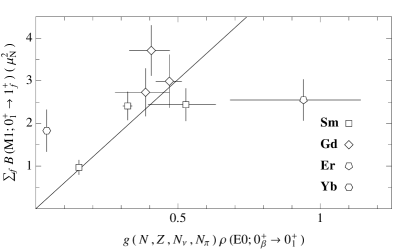
Figure 3: Test of the relation (15) between summed M1 strength and $\rho({\rm E}0;0^{+}_{\beta}\rightarrow 0^{+}_{1})$ values multiplied with the function $g$ defined in Eq. (16). The summed M1 strength is taken from Ref. Enders05 . The slope of the line is determined by $\eta$, $r_{0}^{2}$, and $g_{\nu}-g_{\pi}$, coefficients that are obtained from a fit to radii, E0 and M1 strength.

The relation (15) is valid only in the SU(3) limit which might jeopardize its use in transitional nuclei. One may nevertheless attempt to apply it to the entire rare-earth region. The ratio $r_{0}^{2}/\eta=3.08$ and the effective charges $e_{\rm n}=0.5e$ and $e_{\rm p}=e$ are determined from a fit to radii Zerguine12 . The correlation (15) can now be tested (see Fig. 3) for the eight nuclei in the rare-earth region where both E0 and M1 properties are known (^150,152,154Sm, ^154,156,158Gd, ¹⁶⁶Er, and ¹⁷²Yb). The ¹⁷²Yb point is conspicuously off the line which calls for a search for E0 strength in this nucleus. The ¹⁶⁶Er point follows from a recent experiment Wimmer09 where the fourth $J^{\pi}=0^{+}$ level at 1934 keV has been identified as the band head of the $\beta$-vibrational band with a sizable E0 matrix element to the ground state.

VII Outlook

This work identified the following three topics for further study. The analysis of the correlation between summed M1 strength and $\rho({\rm E0})$ values should be extended to transitions between $J^{\pi}\neq 0^{+}$ states. Secondly, the relation (15) should be generalized to transitional nuclei. Finally, on the experimental front, there is crying need for precise data on isotope shifts through the shape transition in rare-earth nuclei.

References

- (1) S. Zerguine, P. Van Isacker, A. Bouldjedri, S. Heinze, Phys. Rev. Lett. 101, 022502 (2008).
- (2) S. Zerguine, P. Van Isacker, A. Bouldjedri, Phys. Rev. C 85, 034331 (2012).
- (3) F. Iachello and A. Arima, The Interacting Boson Model (Cambridge University Press, Cambridge, 1987).
- (4) J.N. Ginocchio, Phys. Lett. B 265, 6 (1991).
- (5) K. Heyde, P. von Neumann-Cosel, A. Richter, Rev. Mod. Phys. 82, 2365 (2010).
- (6) K. Heyde, C. De Coster, D. Ooms, A. Richter, Phys. Lett. B 312, 267 (1993).
- (7) N. Pietralla et al., Phys. Rev. C 52, 2317(R) (1995).
- (8) J. Enders, P. von Neumann-Cosel, C. Rangacharyulu, A. Richter, Phys. Rev. C 71, 014306 (2005).
- (9) B. Cheal et al., J. Phys. G 29, 2479 (2003).
- (10) E.W. Otten, Treatise on Heavy-Ion Science. VIII Nuclei Far From Stability, ed. D.A. Bromley (Plenum, New York, 1989) p. 517.
- (11) G. Fricke et al., At. Data Nucl. Data Tables 60, 177 (1995).
- (12) I. Angeli, At. Data Nucl. Data Tables 87, 185 (2004).
- (13) W.G. Jin, Phys. Rev. A 49, 762 (1994).
- (14) J.N. Ginocchio and A. Leviatan, Phys. Rev. Lett. 79, 813 (1997).
- (15) N.A. Smirnova et al., Phys. Rev. C 65, 024319 (2002).
- (16) A.R.H. Subber et al., J. Phys. G: Nucl. Phys. 14, 87 (1988).
- (17) K. Wimmer et al., Conf. Proc. AIP 1090, 539 (2009).