Bound states in a hyperbolic asymmetric double-well

Abstract

We report a new class of hyperbolic asymmetric double-well whose bound state wavefunctions can be expressed in terms of confluent Heun functions. An analytic procedure is used to obtain the energy eigenvalues and the criterion for the potential to support bound states is discussed.

I Introduction

Many problems in physics from astronomy Shod_PRL through to relativity Hartmann_PRB_10 can be reduced down to Heun’s equation (see Hortacsu_arXiv and references therein for a general review). Confluent forms of the Heun differential equation are obtained when two or more of the regular singularities coalesce to form an irregular one. Many potentials for the Schrödinger equation have been shown to transform into the Heun equation and its confluent forms Hartmann_PRB_10 ; Chin ; Charles_JMP_13 ; Hartmann_arXiv .

The asymmetric double-well has been studied across many fields of physics from heterostructures Fujiwara_PRL_97 and Bose-Einstein condensates in a double trap Schumm_Nature_05 to superconducting circuits involving tuneable asymmetric double-wells Simmonds_PRL_04 ; Cooper_PRL_04 ; Johnson_PRL_05 , the latter have attracted a great deal of attention due to their potential use as quantum bits. The asymmetric double-well eigenvalue problem has also been studied via supersymmetry techniques Gangopadhyaya_PRA .

We study theoretically a new class of asymmetric double-well, composed of hyperbolic functions with three fitting parameters. It shall be shown that such a potential allows one to reduce the one dimensional Schrödinger equation down to the confluent Heun equation. An analytic procedure is used to obtain the energy eigenvalues namely, the eigenvalues are found by calculating the zeros of the Wronskian formed by two Frobenius solutions, each one expanded about the confluent Heun equation’s different regular singularities.

II Bound states in a hyperbolic asymmetric double-well

The time independent Schrödinger equation reads

$$-\frac{d\Psi}{dx^{2}}+V\left(x\right)\Psi=\varepsilon\Psi.$$ (1)

Here on in all energies are measured in units of $2m/\hbar^{2}$ and the model potential under consideration, $V\left(x\right)$, is given by

$$V\left(x\right)=\left\{-V_{1}\left[1+\tanh^{2}\left(\frac{x}{L}\right)\right]+\left[V_{2}-V_{3}\tanh\left(\frac{x}{L}\right)\right]\right\}\left[1-\tanh^{2}\left(\frac{x}{L}\right)\right],$$ (2)

where the parameters $V_{1}$, $V_{2}$, $V_{3}$ and $L$ characterize the potential strength and width. For the case of $V_{1}=V_{3}=0$, the potential becomes the Pöschl-Teller potential which can be solved exactly, and the wavefunctions are given in terms of Legendre functions Poschl . For the case of $V_{3}=0$, the potential becomes the Manning potential Manning_CP_35 which can be used to describe a harmonic double-well. Substituting equation (2) into equation (1) and making the change of variable $\xi=\left[1+\tanh\left(z\right)\right]/2$ allows equation (1) to be written as

$$4\xi^{2}\left(1-\xi\right)^{2}\frac{\partial^{2}\Psi}{\partial\xi^{2}}+4\xi\left(1-\xi\right)\left(1-2\xi\right)\frac{\partial\Psi}{\partial\xi}-4\xi\left(1-\xi\right)\left[-4w_{1}\xi^{2}+2\left(2w_{1}-w_{3}\right)\xi-2w_{1}+w_{2}+w_{3}\right]\Psi=E\Psi$$ (3)

where we use the dimensionless variable $z=x/L$ with $w_{i}=L^{2}V_{i}$, $i=1,\,2,\,3$ and $E=-L^{2}\varepsilon$. Using the transformation $\Psi=\xi^{q}\left(1-\xi\right)^{r}e^{s\xi}H$ allows equation (3) to be reduced to

$$\frac{\partial^{2}H}{\partial\xi^{2}}+\left[\alpha+\frac{1+\beta}{\xi}+\frac{1+\gamma}{\xi-1}\right]\frac{\partial H}{\partial\xi}+\frac{\mu\xi+\nu}{\xi\left(\xi-1\right)}H=0$$ (4)

where

$$\mu = \delta+\alpha\left(\frac{\beta+\gamma+2}{2}\right)$$

$$\nu = \eta+\frac{\beta}{2}+\frac{\left(\gamma-\alpha\right)\left(\beta+1\right)}{2}$$

and $q$ can take upon the values $\pm\frac{1}{2}\sqrt{E}$ while $s$ can take upon the values $\pm 2\sqrt{w_{1}}$. For the case of $r=q$

$$\alpha=2s\qquad\beta=\gamma=2q\qquad\delta=-2w_{3}\qquad\eta=-2w_{1}+w_{2}+w_{3}+\frac{E}{2}$$

while for $r=-q$

$$\alpha=2s\qquad\beta=2q\qquad\gamma=-2q\qquad\delta=-2w_{3}\qquad\eta=-2w_{1}+w_{2}+w_{3}+\frac{E}{2}.$$

equation (4) has regular singularities at $\xi=0$ and $1$, and an irregular singularity of rank $1$ at $\xi=\infty$. $H$ is the confluent Heun function Heun ; Ronveaux given by the expression

$$H=H\left(\alpha,\,\beta,\,\gamma,\,\delta,\,\eta,\,\xi\right)=\sum_{n=0}^{\infty}c_{n}\xi^{n}$$

where the coefficients $c_{n}$ obey the three term recurrence relation

$$A_{n}c_{n}=B_{n}c_{n-1}+C_{n}c_{n-2}$$

with the initial conditions $c_{n-1}=0$ and $c_{n}=1$ where

$$A_{n} = 1+\frac{\beta}{n}$$

$$B_{n} = 1+\frac{1}{n}\left(\beta+\gamma-\alpha-1\right)+\frac{1}{n^{2}}\left[\eta-\frac{1}{2}\left(\beta+\gamma-\alpha\right)-\frac{1}{2}\beta\left(\alpha-\gamma\right)\right]$$

$$C_{n} = \frac{\alpha}{n^{2}}\left(\frac{\delta}{\alpha}+\frac{\beta+\gamma}{2}+n-1\right).$$

The solutions to equation (3) are therefore given by

$$\Psi_{1}=D_{1}\xi^{q}\left(1-\xi\right)^{q}e^{s\xi}H\left(2s,\,2q,\,2q,\,-2w_{3},\,-2w_{1}+w_{2}+w_{3}+\frac{E}{2},\,\xi\right)$$ (5)

$$\Psi_{2}=D_{2}\xi^{q}\left(1-\xi\right)^{-q}e^{s\xi}H\left(2s,\,2q,\,-2q,\,-2w_{3},\,-2w_{1}+w_{2}+w_{3}+\frac{E}{2},\,\xi\right)$$ (6)

where $D_{1}$ and $D_{2}$ are constants.

Under certain conditions the confluent Heun function can be reduced to a finite polynomial of order $N$. This occurs when two criteria are met Ronveaux :

$$\delta=-\alpha\left(N+1+\frac{\beta+\gamma}{2}\right)$$ (7)

and

$$c_{N+1}=0$$ (8)

where $N$ is a positive integer. Analytic expressions for the energy eigenvalues can be obtained from equation (7) with the caveat that the potential parameters $w_{1}$, $w_{2}$ and $w_{3}$ are interrelated such that the second termination condition, equation (8) is satisfied. In this instance, the potential belongs to a class of quantum models which are quasi-exactly solvable Turbiner_JETP_88 ; Ushveridze_94 ; Bender_JPA_98 ; Charles_JMP_13 ; Hartmann_arXiv , where only some of the eigenfunctions and eigenvalues are found explicitly. This method has been applied to calculate the energy levels in various symmetric hyperbolic double-wells Chin ; Charles_JMP_13 . To determine the bound state energies for a potential described by an arbitrary set of potential parameters we require that the wavefunction vanishes at infinity i.e. $\Psi\left(\xi=0\right)=\Psi\left(\xi=1\right)=0$. However, the function $H\left(\alpha,\,\beta,\,\gamma,\,\delta,\,\eta,\,\xi\right)$ is only analytic within the disk $\left|\xi\right|<1$. An analytic continuation of the confluent Heun function can be obtained by expanding the solution about the second regular singularity $\xi=1$. By relating the two Frobenius solutions one can obtain the bound state energies for arbitrary values of the parameters. The second set of solutions can be constructed by making the change of variable $\xi^{\prime}=1-\xi$, in this instance equation (4) becomes

$$\frac{\partial^{2}H}{\partial\xi^{\prime 2}}+\left[\widetilde{\alpha}+\frac{1+\widetilde{\beta}}{\xi^{\prime}}+\frac{1+\widetilde{\gamma}}{\xi^{\prime}-1}\right]\frac{\partial H}{\partial\xi^{\prime}}+\frac{\widetilde{\mu}\xi^{\prime}+\widetilde{\nu}}{\xi^{\prime}\left(\xi^{\prime}-1\right)}H=0.$$ (9)

For the case of $r=q$

$$\tilde{\alpha}=-2s\qquad\tilde{\beta}=\tilde{\gamma}=2q\qquad\tilde{\delta}=2w_{3}\qquad\tilde{\eta}=-2w_{1}+w_{2}-w_{3}+2q^{2}$$

while for $r=-q$

$$\tilde{\alpha}=-2s\qquad\tilde{\beta}=-2q\qquad\tilde{\gamma}=2q\qquad\tilde{\delta}=2w_{3}\qquad\tilde{\eta}=-2w_{1}+w_{2}-w_{3}+2q^{2}.$$

The solutions to equation (3) are therefore given by

$$\Psi_{3}=D_{3}\xi^{q}\left(1-\xi\right)^{q}e^{s\xi}H\left(-2s,\,2q,\,2q,\,2w_{3},\,-2w_{1}+w_{2}-w_{3}+2q^{2},\,1-\xi\right)$$ (10)

$$\Psi_{4}=D_{4}\xi^{q}\left(1-\xi\right)^{-q}e^{s\xi}H\left(-2s,\,-2q,\,2q,\,2w_{3},\,-2w_{1}+w_{2}-w_{3}+2q^{2},\,1-\xi\right)$$ (11)

where $D_{3}$ and $D_{4}$ are constants.

For $\Psi_{1}$ and $\Psi_{3}$ to be non-divergent functions we require that $q=\frac{1}{2}\sqrt{E}$. $\Psi_{2}$ ($\Psi_{4}$) requires $q=-\frac{1}{2}\sqrt{E}$ ($q=\frac{1}{2}\sqrt{E}$) and that the confluent Heun function is reduced to a confluent Heun polynomial of the order $N$, where $N>\left|q\right|$ . Equation (5) and equation (10) alone are sufficient to determine the eigenvalue spectrum. The solution about $\xi=0$ is convergent for $\left|\xi\right|<1$ where as the solution about $\xi=1$ is convergent for $\left|\xi^{\prime}\right|<1$. Therefore providing $z=z_{1}$ lies in both the analytic domains of $\Psi_{1}$ and $\Psi_{3}$ one can write

$$\Psi_{1}\left(z_{1}\right)=\Psi_{3}\left(z_{1}\right)$$ (12)

For the function to be continuous we also require

$$\left.\frac{\partial\Psi_{1}}{\partial z}\right|_{z=z_{1}}=\left.\frac{\partial\Psi_{3}}{\partial z}\right|_{z=z_{1}}.$$ (13)

Combining equation (12) and equation (13) yields

$$W\left(\Psi_{1},\,\Psi_{3}\right)\left(z_{1}\right)=\left|\begin{array}[]{ccc}\Psi_{1}&\Psi_{3}\\ \frac{\partial\Psi_{1}}{\partial z}&\frac{\partial\Psi_{3}}{\partial z}\end{array}\right|=0.$$ (14)

The energy eigenvalues are therefore obtained by finding the zeros of equation (14). The Wronskian is comprised of two confluent Heun functions each corresponding to the Frobenius solutions about the two regular singularities. In figure 1, we plot $W\left(\Psi_{1},\,\Psi_{3}\right)$ with $z_{1}=0.2$ for the potential parameters $w_{1}=15$, $w_{2}=12$ and $w_{3}=1$ as a function of $E$. The potential is found to contain three bound states at energies $E=0.311$, $2.434$ and $3.875$. The corresponding energy level diagram and normalized wavefunctions are shown in figure 2 and 3 respectively.

III Discussion

The number of bound states contained within the potential is a function of potential strength and width. However, it should be noted that not all combinations of $w_{i}$ result in a potential that can support bound states (see figure 4). Apart from the trivial case wherein combinations of $w_{i}$ result in a purely positive potential across the whole domain of $z$ (thus the potential contains no bound states) there are combinations of $w_{i}$ which gives rise to potentials which are insufficiently deep and or wide to contain a bound state. The critical values of the potential parameters $w_{i}$ which guarantees the existence of a bound state are non-trivial. The threshold conditions are obtained by setting $E=0$ and $z=z_{1}$ and then calculating the zeros of equation (14) as a function of $w_{i}$. The zeros of the Wronskian correspond to the values of $w_{i}$ for which a bound state emerges from the continuum. By determining the values of $w_{i}$ for which the first bound state emerges gives the critical values of $w_{i}$ which guarantees the existence of a bound state. It can be seen from figure 4 that the combination $w_{1}=15$, $w_{2}=12$ and $w_{3}=1$ lies to the right of the critical values of $w_{i}$ which correspond to the emergence of the fourth bound state, therefore the said potential contains only three bound states.

IV Conclusion

It has been shown that a new class of hyperbolic asymmetric double-well can be solved in terms of confluent Heun functions. An analytic procedure for finding the eigenvalues via the calculation of the zeros of the Wronskian, constructed from the two different Frobenius expansions about the two regular singularities have been presented. The criterion for the potential to support bound states was discussed. It is hoped that this model potential, with its easily found energy levels and multiple fitting parameters will serve as a useful tool in the study of phenomena whose behavior is described by asymmetric double-wells.

References

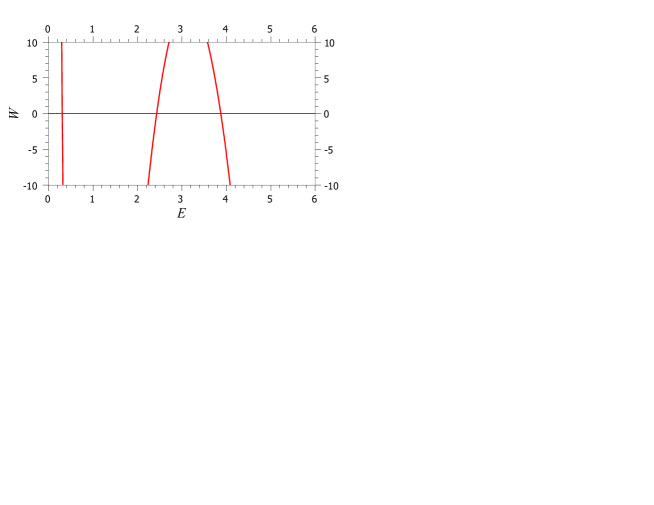
Figure 1: The Wronskian, equation (14), shown in red, for the hyperbolic asymmetric double-well as a function of $E$ with $z_{1}=0.2$ for the case of the potential parameters $w_{1}=15$, $w_{2}=12$ and $w_{3}=1$. The energy eigenvalues are found when the function $W\left(\Psi_{1},\,\Psi_{3}\right)$ is zero this occurs at $E=0.311$, $2.434$ and $3.875$. The $W=0$ (in blue) is shown as a guide to the eye.

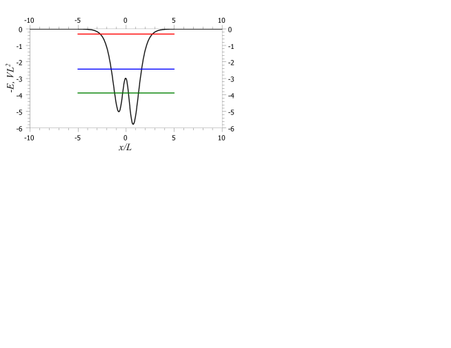
Figure 2: Schematic diagram of the eigenvalue spectrum for the hyperbolic asymmetric double-well described by the parameters $w_{1}=15$, $w_{2}=12$ and $w_{3}=1$, in this instance there are three eigenvalues: $E=0.311$, $2.434$ and $3.875$ and the potential profile is shown in the same scale.

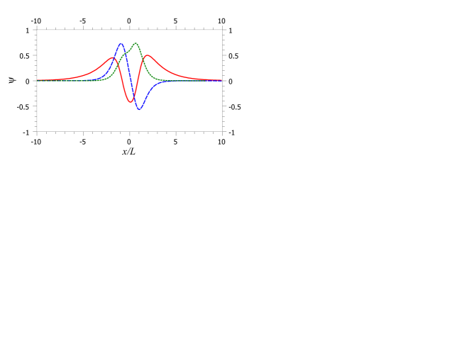
Figure 3: The wavefunctions of the bound states contained within the hyperbolic asymmetric double-well described by the parameters $w_{1}=15$, $w_{2}=12$ and $w_{3}=1$. The solid (red), long-dashed (blue) and short-dashed (green) lines correspond to the $E=0.311$, $2.434$ and $3.875$ eigenvalues respectively.

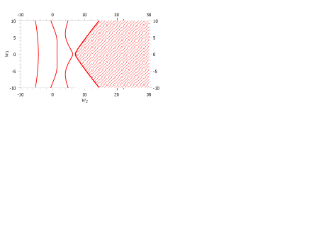
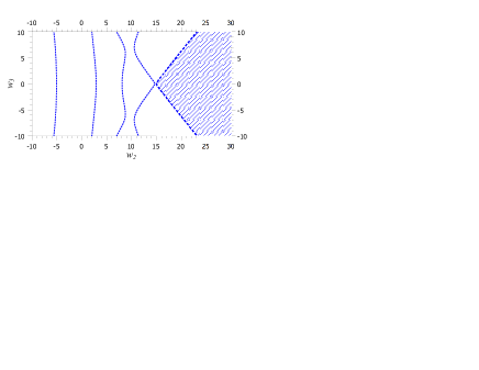
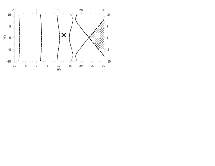
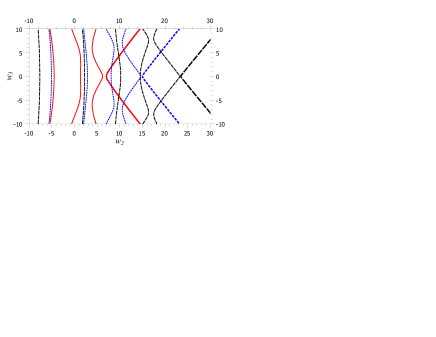
Figure 4: The combinations of $w_{2}$ and $w_{3}$ which gives rise to potentials which do not contain a bound state are shown for the case of $w_{1}=5$ (shaded in red), $w_{1}=10$ (shaded in blue) and $w_{1}=15$ (shaded in black). The threshold values of $w_{i}$ for which new bound states emerge from the continuum are also shown by the solid (red), short-dashed (blue) and long-dashed (black) lines which correspond to $w_{1}=5$, $10$ and $15$ respectively. The critical values of $w_{i}$ which assures that the potential contains a bound state, i.e. the emergence of the first bound state from the continuum, are denoted by the thick lines. The cross corresponds to the potential defined by the combination $w_{1}=15$, $w_{2}=12$ and $w_{3}=1$.

References

• (1) S. Hod, Phys. Rev. Lett. 100, 121101 (2008)
• (2) R. R. Hartmann, N. J. Robinson and M. E. Portnoi, Phys. Rev. B 81, 245431 (2010)
• (3) M. Hortaçsu, arXiv:1101.0471 (2011)
• (4) X. Qiong-Tao, J. Phys. A: Math. Theor. 45, 175302 (2012)
• (5) C. A. Downing, J. Math. Phys. 54, 072101 (2013)
• (6) R. R. Hartmann and M. E. Portnoi, arXiv:1305.4652 (2013)
• (7) K. Fujiwara, S. Hinooda and K. Kawashima, Appl. Phys. Lett. 71, 113 (1997)
• (8) T. Schumm, S. Hofferberth, L. M. Andersson, S. Wildermuth, S. Groth, I. Bar-Joseph, J. Schmiedmayer and P. Krüger, Nature Phys. 1, 57 (2005)
• (9) R. W. Simmonds, K. M. Lang, D. A. Hite, S. Nam, D. P. Pappas and J. M. Martinis, Phys. Rev. Lett. 93, 077003 (2004)
• (10) K. B. Cooper, M. Steffen, R. McDermott, R. W. Simmonds, S. Oh, D. A. Hite, D. P. Pappas and J. M. Martinis, Phys. Rev. Lett. 93, 180401 (2004)
• (11) P. R. Johnson, W. T. Parsons, F. W. Strauch, J. R. Anderson, A. J. Dragt, C. J. Lobb and F. C. Wellstood, Phys. Rev. Lett. 94, 187004 (2005)
• (12) A. Gangopadhyaya, P. K. Panigrahi, and U. P. Sukhatme, Phys. Rev. A 47, 2720 (1993)
• (13) G. Pöschl and E. Teller Bemerkungen zur Quantenmechanik des anharmonischen Oszillators Zeitschrift für Physik 83 (3-4) 143-151 (1933)
• (14) M. F. Manning, J. Chem. Phys. 3, 136 (1935)
• (15) K. Heun, Math. Ann. 33, 161 (1889)
• (16) A. Ronveaux (ed) Heun’s Differential Equations (Oxford: Oxford University Press) (1995)
• (17) A. V. Turbiner, Sov. Phys. JETP 67, 230 (1988); A. Turbiner, Commun. Math. Phys. 118, 467 (1988).
• (18) A. G. Ushveridze, Quasi-exactly Solvable Models in Quantum Mechanics (Taylor and Francis, New York, 1994).
• (19) C. M. Bender and S. Boettcher, J. Phys. A 31, L273 (1998).
Refer to caption