Solar Irradiance Variability and Climate

Abstract

The brightness of the Sun varies on all time scales on which it has been observed, and there is increasing evidence that it has an influence on climate. The amplitudes of such variations depend on the wavelength and possibly on the time scale. Although many aspects of this variability are well established, the exact magnitude of secular variations (going beyond a solar cycle) and the spectral dependence of variations are under discussion. The main drivers of solar variability are thought to be magnetic features at the solar surface. The climate reponse can be, on a global scale, largely accounted for by simple energetic considerations, but understanding the regional climate effects is more difficult. Promising mechanisms for such a driving have been identified, including through the influence of UV irradiance on the stratosphere and dynamical coupling to the surface. Here we provide an overview of the current state of our knowledge, as well as of the main open questions.

1 INTRODUCTION

The Sun is a very special star. Not only is it a boon to astronomers in that it allows us to start resolving spatial scales at which universal physical processes take place that act also in other astronomical objects. It is also the only star that directly influences the Earth and thus also our lives.

Of the many ways in which the Sun affects the Earth, the most obvious is by its radiation. The approximately 1361 Wm^-2 received from the present day Sun at 1 AU (the total solar irradiance, see below) are responsible for keeping the Earth from cooling off to temperatures that are too low for sustaining human life. The composition, structure and dynamics of the Earth’s atmosphere also play a very fundamental part by making efficient use (through the greenhouse effect) of the energy input from the Sun.

The total solar irradiance, or TSI, is defined as the total power from the Sun impinging on a unit area (perpendicular to the Sun’s rays) at 1AU (given in units of Wm^-2). The TSI is the wavelength integral over the solar spectral irradiance, or SSI (Wm^-2nm^-1).

Under normal circumstances, the Sun is the only serious external source of energy to Earth. Any variability of the Sun’s radiative output thus has the potential of affecting our climate and hence the habitability of the Earth. The important question is how strong this influence is and in particular how it compares with other mechanisms including the influence of man-made greenhouse gases. Although this has been debated for a long time, the debate is being held with increasing urgency due to the unusual global temperature rise we have seen in the course of the 20th century and particularly during the last 3–4 decades. It is generally agreed that the recent warming is mainly driven by the release of greenhouse gases, foremost among them carbon dioxide, into the Earth’s atmosphere by the burning of fossil fuels (Solomon et al. 2007). However, determining the exact level of warming due to man-made greenhouse gases requires a good understanding of the natural causes of climate change. These natural causes are partly to be found in the climate system itself (which includes the oceans and the land surfaces), partly they come from the Earth’s interior, by the release of aerosols and dust through volcanoes, and partly they lie outside the Earth and are thus astronomical in nature.

A variety of astronomical effects can influence the Earth’s climate. Thus the energetic radiation from a nearby supernova could adversely affect our atmosphere in a dramatic fashion (e.g., Svensmark 2012). Also, modulation of cosmic rays as the Sun passes into and out of spiral arms during its orbit around the galaxy has been proposed to explain slow variations in climate taking place over 100s of millions of years (Shaviv 2002).

However, the most obvious astronomical influence is due, directly or indirectly, to the Sun, which is the source of practically all external energy input into the climate system. The Sun’s influence can follow three different paths: 1) variations in insolation through changes in the Sun’s radiative output itself (direct influence); 2) modulations of the radiation reaching different hemispheres of the Earth through changes in the Earth’s orbital parameters and in the obliquity of its rotation axis (indirect influence); 3) the influence of the Sun’s activity on galactic cosmic rays proposed to affect cloud cover by, e.g., Marsh & Svensmark (2000).

The first of these is generally considered to be the main cause of the solar contribution to global climate change and will be described in greater detail below. We need to distinguish between changes in TSI, i.e. in the energy input to the Earth system, and variations in SSI, particularly in UV irradiance, which can enhance the Sun’s effect by impacting on the chemistry in the Earth’s middle atmosphere.

The second path is now accepted as the prime cause of the pattern of ice ages and the interglacial warm periods that have dominated the longer term evolution of the climate over the past few million years. The various parameters of the Earth’s orbital and rotational motion vary at periods of 23 kyr (precession), 41 kyr (obliquity) and 100 kyr (eccentricity) (e.g., Paillard 2001, Crucifix, Loutre & Berger 2006). The changes in the Earth’s orbit are so slow that they are unlikely to have contributed to the global warming over the last century.

The third potential path builds on the modulation of the flux of galactic cosmic rays by solar magnetic activity. The Sun’s open magnetic flux (i.e. the flux in the field lines reaching out into the heliosphere) and the solar wind impede the propagation of the charged galactic cosmic rays into the inner solar system, so that at times of high solar activity fewer cosmic rays reach Earth. Their connection with climate has been drawn by, e.g., Marsh & Svensmark (2000) from the correlation between the cosmic ray flux and global cloud cover. However, this mechanism still has to establish itself. Thus the CLOUD experiment at CERN has so far returned only equivocal results on the effectiveness of cosmic rays in producing clouds (Kirkby et al. 2011).

In this review we provide an overview of our knowledge of solar irradiance variability and of the response of the Earth’s climate to changes in solar irradiance. Consequently, mechanisms 2 and 3 are not considered further here. A number of earlier reviews have also covered all or aspects of this topic. Thus, overviews of solar irradiance variability have been given by Lean (1997), Fröhlich & Lean (2004), Solanki, Krivova & Wenzler (2005), Domingo et al. (2009), Lean & DeLand (2012), Krivova & Solanki (2012). The solar activity variations underlying irradiance changes have been reviewed by Usoskin (2008), Hathaway (2010), Charbonneau (2010), Usoskin, Solanki & Kovaltsov (2012). Solar irradiance together with the response of the Earth’s atmosphere have been covered by Haigh, Lockwood & Giampapa (2005), Haigh (2007), Gray et al. (2010), Ermolli et al. (2012), cf. the monograph edited by Pap et al. (2004).

In the following we first discuss the measurements of solar irradiance variations, their causes and models aiming to reproduce the data (Sect. 2), followed by an overview of longer term evolution of solar activity and the associated evolution of solar irradiance (Sect. 3). In Sect. 4 we then move to the response of the Earth’s atmosphere to solar irradiance variations, with conclusions being given in Sect. 5.

2 SHORT-TERM SOLAR IRRADIANCE VARIABILITY

2.1 Measurements of TSI and SSI

The measurement of solar irradiance with an accuracy sufficiently high to detect and reliably follow the tiny, 0.1%, changes exhibited by the Sun was a remarkable achievement. In the meantime missions such as COROT (COnvection, ROtation and planetary Transits; Baglin et al. 2002) and Kepler (Borucki et al. 2003) can detect similar levels of fluctuations on myriads of stars, but reliably measuring the variability of the Sun remains a particular challenge because of the immense brightness contrast of the Sun compared with other astronomical objects, so that maintaining photometric calibrations employing comparisons with many stars is difficult at best (although some instruments do employ this technique in the UV).

Figure 1: Space-borne total solar irradiance (TSI) measurements covering the period 1978–2012 after the TRF (TSI Radiometer Facility) corrections. Individual records are shown in different colours, as labelled in the plot. The bottom part of the plot shows the monthly mean sunspot number. Courtesy of G. Kopp (http://spot.colorado.edu/ koppg/TSI/).

Many attempts to measure “the solar constant” preceded the satellite measurements that finally revealed its variability. Pre-satellite measurements of the solar constant obtained absolute values ranging from 1338 Wm^-2 to 1428 Wm^-2 (see reviews by Smith & Gottlieb 1974, Fröhlich & Brusa 1981). These measurements were too inaccurate to detect intrinsic changes in the solar brightness, even though their presence was suspected (e.g., Eddy 1976). Space-borne radiometers (e.g., Hickey et al. 1980, Willson & Hudson 1988, Fröhlich 2006) provide an almost uninterrupted record of TSI since November 1978 (see Fig. 1). These instruments are accurate and stable enough to trace irradiance variability up to the solar cycle timescale, as revealed in Fig. 1 by the similarity of the curves recorded by different instruments. All the curves (with sufficient time resolution) show two striking features: a trend following the solar cycle, with the irradiance being higher during cycle phases with higher activity and short (week-long) dips in irradiance that coincide with the passage of sunspots across the solar disk.

However, the radiometric accuracy of individual TSI measurements was generally poorer than the $\sim 0.1$% solar cycle change, as indicated by the scatter in absolute values in Fig. 1. A discrepancy of roughly 5 W/m², or 0.35%, has been present between the values measured by instruments launched in the 1980s and 1990s and the Total Irradiance Monitor (TIM) on SOlar Radiation & Climate Experiment (SORCE) launched in 2003 (see Fig. 1). This discrepancy appears to have been resolved thanks to recent tests with the TSI Radiometer Facility (TRF), which allows TSI instruments to be validated against a NIST-calibrated (National Institute of Standards and Technology) cryogenic radiometer at full solar power under vacuum conditions before launch. It has been used to calibrate the PREcision MOnitor Sensor (PREMOS) on PICARD (satellite named after the French astronomer Jean Picard), as well as ground-based representatives of the Total Irradiance Monitor (TIM) on SORCE, the Variability of Solar Irradiance and Gravity Oscillations instrument (VIRGO) on Solar Heliospheric Observatory (SoHO) and the Active Cavity Radiometer Irradiance Monitor (ACRIM) on ACRIM-sat (Kopp & Lean 2011, Kopp et al. 2012, Fehlmann et al. 2012). TRF-based tests and corrections brought PREMOS and ACRIM3 into close agreement, to within 0.05%, with TIM (Kopp et al. 2012, Fehlmann et al. 2012). Thus a TSI value of 1360.8$\pm 0.5$ Wm^-2 is currently considered to best represent solar minimum conditions (Kopp et al. 2012).

The discrepancy in absolute values of individual TSI measurements makes it hard to assess irradiance changes on time scales longer than the solar cycle, since individual radiometers rarely covered more than a single solar activity minimum. To trace long-term changes, individual irradiance measurements need to be adjusted to the same absolute scale, which is a non-trivial task due to instrumental degradation, sensitivity changes and other problems. In particular, early sensitivity changes, when a radiometer starts being exposed to sunlight need to be taken into account (e.g., Lee et al. 1995, Dewitte, Crommelynck & Joukoff 2004, Fröhlich 2006), but also sudden changes in calibration or noise-level, like the ones that occurred on the Nimbus-7 Earth Radiation Budget (ERB) instrument (Hoyt et al. 1992, Lee et al. 1995), can complicate a “cross-calibration” process.

Figure 2: Comparison of the three smoothed TSI composites (ACRIM, yellow; IRMB, green and PMOD, red) as well as TSI reconstructed by the SATIRE-S (blue), all normalised to SORCE/TIM at the minimum in December 2008. Gaps in the curves are gaps in the data longer than 27 days. Credit: Ball et al. (2012), reproduced with permission ©ESO.

Consequently, it is not surprising that three different composites have been produced, which are named after the instrument that they take as the basis, or the institute at which the composite is produced: ACRIM (Willson 1997, Willson & Mordvinov 2003), RMIB (named after the Royal Meteorological Institute of Belgium, sometimes also called IRMB in the francophonic tradition; Dewitte et al. 2004) and PMOD (Physikalisch-Meteorologisches Observatorium Davos; Fröhlich 2006). These composites are plotted in Fig. 2 after imposing a temporal filtering to bring out the longer term changes. The composites agree in many respects, e.g., on short time scales, and they also share most of the features on longer time scales.

The most critical difference between them concerns their longer term trends, which become most clearly visible by comparing the TSI levels during activity minima, i.e. at times when different levels of TSI are easily distinguishable. Such long-term changes are particularly interesting in the context of the global climate change as witnessed in the last century, which explains the debate that these differences in trend have sparked. The ACRIM composite shows an upward trend between the minima in 1986 and 1996, whereas TSI decreases from 1996 to 2008. In the RMIB composite, TSI increases from the minimum in 1996 to 2008. The PMOD TSI shows the opposite trend. The differences in the composites and their sources are described in more detail by Fröhlich (2006, 2012). Independent models assuming irradiance variability to be driven by the evolution of the surface magnetic field agree better with the PMOD long-term trend (see Sect. 2.3).

Figure 3: Top: Reference solar spectrum recorded in April 2008 (Woods et al. 2009). Bottom: Relative SSI variability as observed by UARS/SUSIM (red curve; Floyd et al. 2003) between the maximum of cycle 23 (March 2000) and the preceding minimum (May 1996), as well as by SORCE/SOLSTICE (light blue; Snow et al. 2005) and SORCE/SIM (dark blue; Harder et al. 2009) between April 2004 and December 2008. Also shown is the variability between 2000 and 1996 predicted by the SATIRE model (green; Krivova et al. 2009, Krivova, Solanki & Unruh 2011, Sect. 2.3). For each period, averages over one month are used. Negative values are indicated by dotted segments.

Space-based observations of SSI also started in 1978 with the Nimbus-7 Solar Backscatter Ultraviolet radiometer (SBUV; Cebula, DeLand & Schlesinger 1992), and until 2002 were almost exclusively limited to the UV range below 400 nm. They were reviewed by DeLand & Cebula (2008, 2012). DeLand & Cebula (2008) have also collected the earlier UV data and combined them into a single record. The cross-calibration of individual data sets and construction of a self-consistent composite is, however, in this case even more challenging than for the TSI.

First observations in the visible and IR were sporadic (e.g., by the SOLar SPECtrum, SOLSPEC and SOSP, instruments flown on space shuttles or on the EUropean REtrieval CArrier platform; Thuillier et al. 2003, 2004); see also overviews by Thuillier et al. (2009) and Ermolli et al. (2012). These early measurements were used to produce ATLAS (ATmospheric Laboratory for Applications and Science) solar reference spectra ATLAS1 (March 1992) and ATLAS3 (November 1994; Thuillier et al. 2004). More recent solar reference spectra were produced within the Whole Heliosphere Interval (WHI) international campaign during three relatively quiet periods in March–April 2008 (Woods et al. 2009). One of these spectra, produced during the most quiet period (the WHI quiet Sun reference spectrum), is shown in the upper panel of Fig. 3 (on a logarithmic scale to allow for the differences in irradiance in the UV and the visible). The strong emission line is Ly $\alpha$.

Assessment of the SSI variability is complicated and until relatively recently, this was only possible in the UV range, mainly thanks to the two instruments on board the Upper Atmosphere Research Satellite (UARS): the Solar-Stellar Irradiance Comparison Experiment (SOLSTICE; Rottman, Woods & Sparn 1993) and the Solar Ultraviolet Spectral Irradiance Monitor (SUSIM; Brueckner et al. 1993). In the UV below about 250 nm, long-term instrumental uncertainties of SOLSTICE and SUSIM were smaller than the solar variability (e.g., Woods et al. 1996). The lower panel of Fig. 3 illustrates the relative difference in the irradiance spectrum between activity maximum and minimum . Clearly, the irradiance variability is a strong function of wavelength and increases very rapidly towards shorter wavelengths in the UV (note the logarithmic scale). In spite of differences in detail, all data sets show a qualitatively similar behaviour in the UV, illustrated by the red and blue curves. Quantitatively there are differences of up to nearly an order of magnitude, which do not appear so striking due to the logarithmic scaling. They are discussed below.

The results of the Solar Radiation and Climate Experiment (SORCE) launched in 2003 sprang a surprise. SORCE carries two instruments, the SOLSTICE (an analogue of UARS/SOLSTICE, Snow et al. 2005) and the Spectral Irradiance Monitor (SIM, Harder et al. 2005), which observe SSI over a broad spectral range from Ly-$\alpha$ to 2400 nm. Between 2003 and 2008, i.e. over the declining phase of cycle 23, SIM displayed an anticyclic behaviour in the visible, i.e. the irradiance at most visible and IR wavelengths is lower at higher activity levels than during quiet times (Harder et al. 2009). This is indicated by the dotted blue line in Fig.  3. These values whould be negative (which cannot be directly represented on a logarithmic scale). This anti-phase behaviour to the TSI is largely compensated by the enhanced in-phase UV variability between 200 and 400 nm compared with previous measurements. Thus the estimated contribution of the 200–400 nm spectral range to the TSI decrease from 2004 to 2008 was about 180% (Harder et al. 2009), compared with 20-60% based on earlier measurements (Lean et al. 1997, Thuillier et al. 2004, Krivova, Solanki & Floyd 2006, Morrill, Floyd & McMullin 2011).

At the same time, the short-term (rotational) variability measured by SORCE/SOLSTICE and SORCE/SIM agrees with previous results very well. Since shorter time scales are significantly less affected by instrumental effects, DeLand & Cebula (2012) conclude that undercorrection of response changes for the SORCE instruments is the most probable source of the discrepancies.

The importance of getting the correct spectral dependence of the irradiance variations lies in the fact that the UV irradiance influences atmospheric chemistry more strongly than that in the visible, although the visible cannot be neglected (see Sect. 4).

2.2 Physical Causes of Irradiance Variations

Figure 4: Power spectrum of total solar irradiance. The different curves have the following meaning: Fourier (grey line) and global wavelet (black dotted line) power spectra (in ppm${}^{2}/60\mu$Hz) of the VIRGO data set for the year 2002 sampled at a 1 min cadence (Fröhlich et al. 1995). Black solid line shows the global wavelet spectrum of the SORCE TIM data (Kopp, Lawrence & Rottman 2005) for the year 2003 sampled every 6 h. Credit: Seleznyov, Solanki & Krivova (2011), reproduced with permission ©ESO.

There are a variety of causes of solar irradiance variations, each acting on particular timescales. This is illustrated in Fig. 4 for a limited set of timescales by plotting the power spectrum of TSI for periods from about 1 minute to 1 year (Seleznyov, Solanki & Krivova 2011). The power drops very roughly as a power law from long to short time scales. These variations are driven by a range of sources. Thus, solar oscillations, the $p$-modes, are responsible for the group of peaks centered on 5 min (3 mHz), the evolution of granules produces the plateau between 50 and 500 $\mu$Hz (i.e. on periods of minutes to hours), while the rotational modulation of TSI by the passage of sunspots and faculae over the solar disc leads to the increase in power between 0.4 and 50 $\mu$Hz (i.e. periods of between about 5 and 5000 hours). The solar rotation period itself does not display a significant peak in this figure, however, due to the combination of the limited lifetime of sunspots (most live only a few days or less) and the constant evolution of the brightness of the longer lived active regions, as well as the rather common occurance of multiple active regions on the Sun at the same time.

From the solar rotation period to the 10–12 year solar-cycle period the growth, evolution and decay of active regions, as well as the distribution of their remnant magnetic field over the solar surface provide the main contribution to the variability. This is strongly modulated by the activity cycle itself, which is a very strong contributer to irradiance variations. Beyond the solar cycle period, the difference in the strength of individual cycles as well as possible evolution of the background field and other mechanisms (see Sect. 3) may lead to a secular change, which might be visible in the form of different TSI levels at the different minima. Over the thermal relaxation time-scale of the convection zone of $10^{5}$ years the energy blocked by sunspots should be gradually released again (see below), while beyond $10^{6}$ years the gradual brightening of the Sun due to the chemical evolution of its core should start to become noticeable in its TSI (e.g., Sackmann, Boothroyd & Kraemer 1993, Charbonnel et al. 1999, Mowlavi et al. 2012).

With the exception of the shortest and the longest time scales, the causes of irradiance variations listed above are associated more or less directly with the Sun’s magnetic field mainly via the influence of magnetic fields on the thermal structure of the solar surface and atmosphere.

For irradiance variations of possible relevance to global climate change, the magnetic field is expected to be the main driving force. Of importance is the magnetic field at the solar surface and in the lower solar atmosphere, mainly the photosphere (see, e.g., Solanki & Unruh 1998). In these layers the magnetic field is thought to be concentrated into strong field features (having an average field strength of roughly a kG in the mid photosphere; Solanki et al. 1999) whose simplest description is by magnetic flux tubes (see Solanki 1993 for a review), although their real structure is more complicated (e.g., Vögler et al. 2005, Rempel et al. 2009, Stein 2012). Another, more chaotic component of the magnetic field is present as well (see de Wijn et al. 2009 for a review). It is still unclear if this turbulent field component really contributes to irradiance variations, so that in the following we restrict ourselves to the concentrated fields which range in cross-section size between structures well below 100 km in diameter to sunspots that often have dimensions of multiple 10 Mm.

Sunspots, forming the hearts of active regions, clearly are dark (see Solanki 2003, Rempel & Schlichenmaier 2011 for reviews), while the small magnetic elements that populate (and form) the faculae in active regions and the network elsewhere on the Sun (and are even found in the internetwork of the quiet Sun; Sánchez Almeida et al. 2004, Lagg et al. 2010) are bright, particularly near the limb and at wavelengths formed above the solar surface. Such wavelengths include the Fraunhofer g-band (Muller & Roudier 1984, Berger et al. 1995), the CN bandhead (Sheeley 1969, Zakharov et al. 2007), the cores of strong spectral lines (e.g., Skumanich, Smythe & Frazier 1975) and the UV (Riethmüller et al. 2010).

The darkness of sunspots is due to the blocking of heat flowing from below by the kG magnetic field, which is strong enough to largely quench overturning convection (Rempel & Schlichenmaier 2011). Forms of magnetoconvection do take place, maintaining the penumbra’s (and to some extent also the umbra’s) brightness (e.g., Schüssler & Vögler 2006, Rempel et al. 2009, Joshi et al. 2011, Scharmer et al. 2011).

Figure 5: Sketch of the vertical cross-section through a slender magnetic flux tube. The arrows illustrate the various forms of energy transfer. Red arrows: vertical convective and radiative energy flux below the solar surface inside the flux tube (subscript i) and in the external medium (subscript e). Yellow arrows: horizontal influx of radiation through the walls of the flux tube (the thick lines outline the optical depth unity, $\tau=1$, surface, as seen from above). $\Delta Z$ represents the Wilson depression. Green arrows: mechanical energy flux. The cloud sketches the hot chromospheric layers of the magnetic feature (roughly following a sketch by Zwaan 1978).

The magnetic elements have a nearly equally strong field (as sunspots averaged over their cross-section), so that the convective energy flux from below is greatly reduced in their interiors. This is indicated by the different lengths of the vertical red arrows in Fig. 5. This figure displays the vertical cross-section of an intense slender flux tube. Another feature that can be seen in the figure is the depression of the optical depth unity surface (heavy black line) in the flux tube’s interior. Hence, for depths up to $\Delta Z$ below the solar surface in the quiet Sun, the walls of the flux tube allow radiation to escape into space. This radiation heats up the interior of the tube. Forthermore, photons from these hot walls (which are windows into the hot interior of the Sun) can be directly observed, best when the magnetic element is located at some distance away from solar disc centre (Spruit 1976, Keller et al. 2004, Carlsson et al. 2004).

In addition to this radiative heating, the magnetic elements are shaken and squeezed by the turbulently convective gas in their surroundings. This causes the excitation of different wave modes within them (Musielak & Ulmschneider 2003). This mechanical transfer of energy from the surroundings into the tubes is represented in Fig. 5 by the green horizontal arrows, while the upward transport of the mechanical energy by waves is indicated by the vertical green arrow.

In particular the longitudinal tube waves steepen as they propagate upwards, due to the drop in density, finally dissipating their energy at shocks in the chromosphere (e.g., Carlsson & Stein 1997, Fawzy, Cuntz & Rammacher 2012). Other forms of heating may also be taking place, but are not discussed further here. This leads to a heating of the upper photospheric and chromospheric layers of magnetic elements, which explains their excess brightness in the UV and in the cores of spectral lines (e.g. Ca II H and K, see Schrijver et al. 1989, Rezaei et al. 2007).

Whereas the radiation flowing in from the walls penetrates the small magnetic features completely, for features with horizontal dimension greater than roughly 400 km the radiation cannot warm the inner parts and they remain cool and dark, cf. Grossmann-Doerth et al. (1994).

The radiative properties of sunspots (and to a lesser extent the smaller, but still dark pores) and magnetic elements are responsible for most of the irradiance variations on time scales of days to the solar cycle and very likely also beyond that to centuries and millenia, as described in the following sections.

However, one important question remains: Why does the energy blocked by the magnetic field in sunspots not simply flow around them and appear as a surrounding bright ring? Such bright rings have been found (e.g., Waldmeier 1939, Rast et al. 2001), but prove to release only a few percent of the energy flux blocked by the enclosed sunspots. An explanation was provided by Spruit (1982b, a), who showed that the energy blocked by sunspots is redistributed in the solar convection zone due to the very high heat conductivity of the solar plasma (see Spruit 2000 for a review). Due to the very high heat capacity, the stored heat hardly changes the surface properties at all. This heat is gradually re-emitted over the Kelvin-Helmholtz timescale of the convection zone, which is approximately $10^{5}$ yr. In analogy, the excess radiation emitted by magnetic elements also comes from the convection zone’s large heat reservoir. Consequently, one may consider magnetic elements as leaks in the solar surface, since by dint of being evacuated they increase the solar surface area (see Fig. 5).

Alternative explanations to the TSI variations on timescales of the solar cycle and longer have also been proposed, e.g. thermal shadows produced by horizontal magnetic flux in the solar interior (Kuhn et al. 1998) or long-period ($\approx 1$ month) oscillations driven by the Coriolis force (r-modes; Wolff & Hickey 1987). As we shall see in the next subsection, the surface magnetic field leaves at most a few percent of the TSI variations on timescales up to the solar cycle to be explained by these or other such mechanisms. However, it cannot be ruled out that one of these mechanisms (or an as yet unknown one) may contribute significantly on longer time scales (e.g., Sofia & Li 2001).

2.3 Modelling of TSI and SSI

Models assuming that irradiance variations on time scales longer than roughly a day are caused by changes in the surface distribution of different magnetic features (see Sect. 2.2) turned out to be most successful in explaining observed irradiance changes. The first models of this type (e.g., Willson et al. 1981, Oster, Schatten & Sofia 1982, Foukal & Lean 1986) were so-called proxy models, which combined proxies of solar surface magnetic features using regressions to match observed TSI changes. Proxies that have been used most frequently include the sunspot area and the Photometric Sunspot Index (PSI) derived from it (a measure of sunspot darkening), as well as Mg II, Ca II and F10.7 (solar radio flux at 10.7 cm) indices to describe facular brightening. The widely used Mg II index is the ratio of the brightness in the cores of the Mg II lines to their wings, making it relatively insensitive to instrumental degradation with time (Viereck et al. 2001). However, it is sensitive to the exact wavelength choice, which leads to uncertainties in the long-term trend in the composite Mg II record. The Ca II index is similarly defined. More accurate proxy models employ spatially resolved observations of the full solar disc, which account for the center-to-limb variation of spot and facular contrasts at least at one wavelength (e.g. Chapman, Cookson & Dobias 1996, Chapman, Cookson & Preminger 2012, Preminger, Walton & Chapman 2002). More details on proxy models can be found in reviews by Fröhlich & Lean (2004) and Domingo et al. (2009).

With time, more physics-based models have been developed (e.g., Fligge, Solanki & Unruh 2000, Krivova et al. 2003, Wenzler et al. 2006, Shapiro et al. 2010, Ermolli, Criscuoli & Giorgi 2011, Fontenla et al. 2011). They still use different (spatially resolved or disc-integrated) observations or proxies of solar magnetic activity to describe the evolution of the surface coverage by different types of solar feautures (such as spots or faculae), also called components of the solar atmosphere. But the brightness of each component is calculated using radiative transfer codes from semi-empirical models of different features in the solar atmosphere (see, e.g., Kurucz 1993, Fontenla et al. 1999, Unruh, Solanki & Fligge 1999, Fontenla et al. 2009, Shapiro et al. 2010). Brightnesses of the photospheric components computed in this way depend on the wavelength and the heliocentric position. This brings two advantages: 1) it allows calculating the spectral irradiance, which is less straightforward with proxy models, and 2) it takes into account the centre-to-limb variation of the contrasts of different magnetic components, which provides more accurate reconstructions of solar irradiance. A successful example is the SATIRE-S (Spectral And Total Irradiance REconstructions for the Satellite era) model employing daily solar magnetograms and continuum images (Krivova et al. 2003, Wenzler et al. 2006, Ball et al. 2012).

Figure 6: Top: TSI between 1978 and 2009 as given by the PMOD composite record of measurements (light red curve for daily and thick red for smoothed data) and as computed with the SATIRE-S model (light blue and thick blue for daily and smoothed data, respectively). Both data sets are normalised to SORCE/TIM data in December 2008. The thin blue lines indicate the uncertainty range of the model. Dashed horizontal lines mark TSI levels at cycle minima. Dotted vertical lines indicate cycle maxima and minima. Black error bars are the PMOD TSI errors from Fröhlich (2009). Bottom: the difference between PMOD and SATIRE-S TSI (daily, grey; smoothed, black). The PMOD TSI error bars are shown in red. Credit: Ball et al. (2012), reproduced with permission ©ESO.

In the last decade, significant progress has been made in modelling TSI (Preminger, Walton & Chapman 2002, Ermolli, Berrilli & Florio 2003, Krivova et al. 2003, Lean et al. 2005, Wenzler et al. 2006, Ball et al. 2012, Chapman, Cookson & Preminger 2012). State-of-the-art models reproduce more than 90% of the measured TSI variations over the whole period covered by observations (see Fig. 6) and more than 95% for cycle 23 (Ball et al. 2011, 2012, Chapman, Cookson & Preminger 2012), when compared with the PMOD composite (see Sect. 2.1).

The models can in principle be used to distinguish between the composites. On the solar cycle and longer time scales, Wenzler, Solanki & Krivova (2009), Krivova, Solanki & Wenzler (2009) and Ball et al. (2012) found the SATIRE-S model to be in best agreement with the PMOD composite (Fig. 2), although after the removal of long-term trends, the best agreement is reached with the RMIB composite. Kopp & Lean (2011) obtain similar correlations between their proxy model (NRLSSI, see later in this section) and the RMIB ($r_{c}$ = 0.92) and PMOD ($r_{c}$ = 0.91) composites.

Development of climate models including chemistry and thus increased interest in solar UV data has stimulated advances to SSI modelling. Over the years a number of models describing the variation of SSI have been constructed. These include the Naval Research Laboratory Solar Spectral Irradiance model (NRLSSI; Lean et al. 1997, Lean 2000), SATIRE-S (Krivova, Solanki & Floyd 2006, Krivova et al. 2009, Krivova, Solanki & Unruh 2011, Ball 2012), the COSI (COde for Solar Irradiance; Shapiro et al. 2010, 2011), SRPM (Solar Radiation Physical Modelling; Fontenla et al. 1999, 2004, 2009, 2011) and OAR (Osservatorio Astronomico di Roma; Ermolli, Criscuoli & Giorgi 2011, Ermolli et al. 2012) models. Two recent models by Bolduc et al. (2012) and Thuillier et al. (2012) are limited to the UV spectral range only. An overview of SSI models has recently been given by Ermolli et al. (2012).

These models reach different levels of complexity, make partly different assumptions (with the common main underlying assumption being that evolution of the magnetic field at and above the solar surface is the main cause of SSI variability) and show partly significant differences in their results (as discussed below). Nonetheless, they do have some important traits in common that are worth stressing (with one exception, the SRPM model by Fontenla et al. 2011, discussed later in this section).

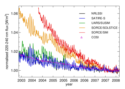
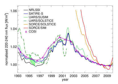
Figure 7: Normalised solar UV irradiance between 220 and 240 nm calculated with NRLSSI (black), SATIRE-S (blue) and COSI (magenta), and measured with UARS/SUSIM (darker green), UARS/SOLSTICE (light green), SORCE/SOLSTICE (orange) and SORCE/SIM (red). The pale green shading marks the period when the sensitivity of the UARS/SUSIM instrument (and thus the flux) changed, so that a shift was applied to the data before that (see Krivova, Solanki & Floyd 2006, Krivova et al. 2009 for details). Left-hand panel is limited to the period when SORCE was in operation, i.e. after 2003, and shows daily values, except for the COSI model, for which only yearly averages are available. Right-hand panel shows 3-month smoothed values over the period 1993–2009, for which UARS and/or SORCE data are available. From Ermolli et al. (2012).

1. All models produce a generally increasing level of SSI variability with decreasing wavelength in the UV. This is in qualitative agreement with the measurements (see bottom panel of Fig. 3), while quantitative comparisons are discussed below.

2. On solar rotation timescales the models and data agree remarkably well, at least for the more advanced models. This is illustrated by the left-hand panel of Fig. 7, which shows daily normalised SORCE data (SIM in red and SOLSTICE in orange), UARS/SUSIM data (green) and four different models in the spectral range 220–240 nm over the period 2003–2009.

3. On the solar cycle time-scale the UV variability displayed by all models is much lower (by factors of 2–6) than that shown by the SSI instruments on SORCE, although for the more advanced models it agrees rather well with the variations found by the SSI instruments on UARS. The right-hand panel of Fig. 7 shows 3-month smoothed values of solar irradiance at 220–240 nm between 1993 and 2009, calculated with the NRLSSI (black curve), SATIRE-S (blue) and COSI (magenta; yearly values) models and measured by UARS/SOLSTICE (darker green), UARS/SUSIM (lighter green), SORCE/SOLSTICE (orange) and SORCE/SIM (red). In this spectral range, all three models agree well with each other over the whole period 1993–2008, as well as with the UARS data between 1993 and 2005 (SUSIM stopped its operation in August 2005, UARS/SOLSTICE in 2002). But the 220–240 nm flux measured by the SORCE instruments over the period 2004–2008 decreased by a factor of 4 (SOLSTICE) to 7 (SIM) more than expected from the models. The difference between the trend measured by SORCE/SOLSTICE and reconstructed by the models actually lies within the 3-$\sigma$ long-term instrumental uncertaity (Unruh, Ball & Krivova 2012). The discrepancy between the models and SIM is larger, but in this spectral range SIM is considered to be less accurate than SOLSTICE.

4. The SSI variability is in phase with the solar cycle at all wavelengths (with the exception of a short stretch in the IR). This disagrees with the data from SORCE/SIM (cf. the green curve, showing the SATIRE-S model, and the dotted part of the blue curve showing SIM data at antiphase with the cycle in Fig. 3).

Although qualitatively the results of most models are similar, they also show significant quantitative differences. Most important for climate models is the discrepancy in the estimated UV variability at 250–400 nm, where models differ by up to a factor of three, e.g. between NRLSSI and COSI. On the one hand, proxy models generally tend to underestimate the variability in this range. Such models rely on SSI measurements, at least in this spectral range (e.g., NRLSSI and the models by Pagaran, Weber & Burrows 2009 or Thuillier et al. 2012), and extrapolate observed rotational variability to longer time scales.

On the other hand, model atmospheres of the solar features employed in semi-empirical SSI models (e.g., in SATIRE-S, COSI, SRPM, OAR) have not yet been tested observationally at all wavelengths (due to the lack of appropriate observations) and have some freedom as well, although they cannot be tuned arbitrarily. An example is given by the SRPM model (Fontenla et al. 2011), in which the atmospheric models were tuned to allow better agreement with the SORCE SSI data. Thus it is the only model, which qualitatively reproduces SORCE/SIM SSI behaviour, in particular, the reversed variability in the visible. This is, however, achieved at the expense of TSI: the modelled TSI does not reproduce the solar cycle change, which is measured much more reliably than the SSI. Interestingly, the OAR model uses essentially the same input as SRPM, with the earlier untuned versions of the same atmospheric models (Fontenla et al. 2009) and is able to reproduce the TSI changes, but not the SORCE SSI variability (Ermolli et al. 2012). The difference in the predicted variability at 250–400 nm between semi-empirical models (excluding SRPM, i.e. considering only models that reproduce the TSI variability) is still almost a factor of two, with COSI showing the strongest variability and OAR the weakest. A more detailed comparsion of the models has been presented by Ermolli et al. (2012).

3 LONGER TERM SOLAR VARIABILITY: SECULAR CHANGE OF IRRADIANCE

3.1 Grand Maxima and Minima

The longest running record of solar activity, available since 1610, is the sunspot number (observations started only one year after the invention of the telescope in 1609). It is a simple measure of the Sun’s activity, but nonetheless rather robust, especially when only sunspot groups are counted (as is the case for the group sunspot number introduced by Hoyt & Schatten 1998). Robustness is a necessary condition since data from different sources need to be combined in building up any long-running solar activity record. The most striking feature of this record, plotted in Fig. 8, is the solar activity cycle. Each cycle lasts between 8 and 14 years, with an average length of approximately 11.2 years. Cycle amplitudes vary even more strongly, with the weakest known cycle (starting around 1700) being less than 10% in strength of the strongest cycle, cycle 19, although in the minima between the cycles the sunspot number reaches nearly zero (there are some differences between minima following very strong and those following weaker cycles). The solar cycle has been reviewed in detail by Hathaway (2010).

Figure 8: Telescopic, yearly averaged, sunspot number records: Zurich (orange) and group sunspot number (blue; Vaquero et al. 2011, Hoyt & Schatten 1998, SIDC 2011). The Zurich (or Wolf) number was introduced by Rudolf Wolf in the 1840s, the group number by Hoyt & Schatten (1998). The group sunspot number has been proposed to better represent actual level of activity before 1880, but is not yet officially available for cycles 23 and 24.

Almost as striking as the presence of the cycles is their absence, along with the near absence of sunspots themselves, between roughly 1640 and 1700 (Eddy 1976, Soon & Yaskell 2003). This Maunder minimum is a prime example of a grand minimum of solar activity, which in this case overlapped with a particularly cold part of the little ice age. Grand minima of solar activity have been reviewed by Usoskin, Solanki & Kovaltsov (2012).

The only direct records of solar activity measurements that reach further back in time are scattered naked-eye sightings of sunspots, mainly in China (Yau & Stephenson 1988). These are too scarce to allow a reliable reconstruction of solar activity. An alternative is provided by cosmogenic isotopes, such as ¹⁴C and ¹⁰Be stored in terrestrial archives. These isotopes are produced in the Earth’s atmosphere by nuclear reactions (neutron capture, spallation) between energetic cosmic rays and constitutents of the Earth’s atmosphere (mainly N, but also O and Ar in the case of ¹⁰Be). After production the two main cosmogenic isotopes take different paths. ¹⁴C becomes part of the global carbon cycle until it ends up in one of the sinks, e.g. the ocean or in plant material. Of interest are those atoms that end up in the trunks of datable trees. After circulating in the atmosphere for a few years, if it was formed in the stratosphere, ¹⁰Be precipitates and can be recovered (and dated) if it is deposited on striated ice sheets, such as those of Greenland or Antarctica.

Since both isotopes are radioactive (half-lives of 5730 years for ¹⁴C, and $1.36\times 10^{6}$ years for ¹⁰Be) and have no terrestrial sources, their concentration in a layer (or year-ring) of their natural archives is a measure of the production rate of these isotopes at the time of deposition (after relevant corrections). This in turn depends on the flux of cosmic rays reaching the Earth’s atmosphere, which is mainly determined by the strength (and, at least for ¹⁰Be, the geometry) of the Earth’s magnetic field, and on the level of solar activity. Hence, if the geomagnetic field is known from a previous reconstruction (e.g. Korte & Constable 2005, Knudsen et al. 2008), then the level of solar activity, primarily modulation potential, which depends mainly on the Sun’s open magnetic flux, can be determined using a simple model.

A further important requirement for ¹⁴C is that ocean circulation remains roughly unchanged (which can be shown for the Holocene, Stuiver 1991). The ¹⁰Be, in turn, may be sensitive to variations in local climate (e.g. Field et al. 2006).

The connection of the open magnetic flux with the quantities needed to estimate solar irradiance variations, sunspot and facular areas, or alternatively sunspot number and total magnetic flux, can then be established via another simple model introduced by Solanki, Schüssler & Fligge (2000, 2002), cf. Vieira & Solanki (2010). The main ingredient of this model is that solar cycles overlap due to two mechanisms: (1) magnetic flux belonging to the new cycle starts to emerge while flux belonging to the old cycle is still emerging and (2) magnetic flux organized on large scales (i.e. mainly the open flux) decays very slowly, over a timescale of years, and hence is still present when the next cycle is well underway.

Usoskin et al. (2004) have shown that by putting together the various models solar activity can be reconstructed reliably, at least from ¹⁴C. This was put to use by Usoskin et al. (2003b), who reconstructed sunspot number for the last 1000 years, and by Solanki et al. (2004), who did that for the last 11400 years, i.e. basically the full holocene. Reconstructions of solar activity based on ¹⁰Be followed later (Steinhilber, Abreu & Beer 2008, Steinhilber, Beer & Fröhlich 2009). Although the reconstructions based on the two isotopes (and to some extent those based on different geomagnetic field reconstructions) differ from each other in detail, they show a similar statistical behaviour (Usoskin et al. 2009, Steinhilber et al. 2012). Such model-based reconstructions supercede earlier work by, e.g., Stuiver & Braziunas (1989) with ¹⁴C.

Figure 9: Sunspot number for the last 11400 years reconstructed from ¹⁴C. The original 10-year sampled data have been smoothed with a 1-2-2-2-1 filter prior to plotting. Red and blue areas denote grand maxima and minima, respectively. Credit: Usoskin, Solanki & Kovaltsov (2007), reproduced with permission ©ESO.

The reconstructed (smoothed) sunspot number is plotted in Fig. 9. Clearly, there have been a number of periods of very low activity similar to the Maunder minimum. Those with the sunspot number below 15 for at least 20 years are defined as grand minima, while the sunspot number above 50 for the same length of time gives a grand maximum. Other definitions are also possible (see, e.g., Abreu et al. 2008).

Grand minima and maxima are almost randomly distributed, although grand minima tend to come in clusters separated by roughly 2000–3000 years. Unlike the grand maxima, whose duration follows an exponential distribution, the grand minima come in two varieties, a short (30–90 year) type, with the Maunder minimum being a classic example, and a long ($>110$ year) type, such as the Spoerer minimum (1390–1550).

The last grand maximum of solar activity has only just ended. As Usoskin et al. (2003a) and Solanki et al. (2004) showed, the Sun entered in a grand maximum in the middle of the 20th century, characterized by strong sunspot cycles, short, comparitively active minima, a high value of the Sun’s open magnetic flux and plentiful other indicators of vigorous solar activity. This grand maximum has now ended as had been expected by Solanki et al. (2004) and later by Abreu et al. (2008). This is indicated by the long and very quiet activity minimum between cycles 23 and 24 (2005–2010) and the weak currently running cycle.

Making predictions about how the activity will develop in future is not at present possible beyond the maximum of the current cycle. Thus only statistical estimates of future solar activity can be made based on comparisons with the reconstructed long-term activity record (Solanki et al. 2004, Abreu et al. 2008, Lockwood 2009, Solanki & Krivova 2011). In particular, it is unlikely that the Sun will slip into a grand minimum (less than 8% likelihood within the next 30 years, Lockwood 2009) and it is equally likely that the next grand extremum will be a grand maximum as a grand minimum.

3.2 By How Much Did the Sun Vary Between the Maunder Minimum and Now?

Figure 10: Various TSI reconstructions since 1600 identified in the plot. The dark blue vertical bar shows the possible range of the TSI change following Schrijver et al. (2011, see text, no reconstruction available). Other vertical bars denote uncertainties of the models, plotted in same colours. Note that the uncertainty in the Shapiro et al. 2011 model, $\pm 3$ Wm^-2, extends downward outside the plot, and the blue horizontal bar and arrow mark the reduced value of this model as argued by Judge et al. (2012). The black dotted line shows the TSI value representing solar minimum conditions following SORCE/TIM measurements (see Sect. 2.1).

The sunspot number is a good representative of the solar magnetic activity cycle. Hence historical records of sunspot number since 1610 (Hoyt & Schatten 1998) and sunspot areas since 1874 (e.g., Balmaceda et al. 2009, and references therein) allow decent reconstructions of the cyclic component of solar irradiance changes over the last four centuries. All such reconstructions show that in the last few decades the Sun was unusually active (see previous section), so that the cycle-average TSI was also roughly 0.6 Wm^-2 higher than during the Maunder minimum (Solanki & Fligge 2000) even in the absence of any secular change.

Reconstructions of the heliospheric magnetic field from the geomagnetic aa-index and observations of the interplanetary magnetic field imply that the Sun’s open magnetic field increased by nearly a factor of two since the end of the 19th century (Lockwood, Stamper & Wild 1999, Lockwood, Rouillard & Finch 2009) before dropping again to the 19th century values in the last few years. The total photospheric magnetic flux, which is more directly related to solar irradiance, has been regularly measured for only about four decades (e.g. Arge et al. 2002, Wang, Sheeley & Rouillard 2006), so that longer-term changes cannot yet be reliably assessed. Harvey (1993, 1994) noticed, however, that small ephemeral active regions keep bringing copious amounts of magnetic flux to the solar surface during activity minima, when active regions are rare or absent. The magnetic flux provided by the ephemeral regions, and concentrated in the network in the quiet Sun, varies little over the activity cycle as ephemeral regions belonging to two different solar cycles emerge in parallel for multiple years (Harvey 1992, 1993, 1994, Hagenaar, Schrijver & Title 2003). The overlap between the cycles provides a physical explanation for the secular change in the photospheric magnetic field and irradiance (Solanki, Schüssler & Fligge 2000, 2002).

The magnitude of the secular change remains, however, heavily debated. This is because the sunspot numbers or areas widely employed in the reconstructions on time scales longer than a few decades are related only indirectly to the amount of flux emerging in small ephemeral regions feeding the magnetic network.

The first estimates of the TSI change since the Maunder minimum, mainly derived from solar-stellar comparisons, ranged from 2 to 16 Wm^-2 (Lean, Skumanich & White 1992, Zhang et al. 1994, Mendoza 1997). They were indirect and based on a number of assumptions that were later found to be spurious (e.g., Wright 2004, Hall & Lockwood 2004, Hall et al. 2009). Judge et al. (2012) argue that current stellar data do not yet allow an assessment of the secular change in the solar brightness, and longer stellar observations are required.

Various empirical reconstructions produced in the 2000s give values between 1.5 and 2.1 Wm^-2 (e.g., Foster 2004, Lockwood 2005, Mordvinov et al. 2004). Lockwood & Stamper (1999) were the first to apply a linear relationship between the open magnetic flux and the TSI derived from the data obtained over the satellite period. Later, such a linear relationship was also employed by Steinhilber, Beer & Fröhlich (2009) to reconstruct TSI from the ¹⁰Be data. This reconstruction covers the whole Holocene and is discussed in Sect. 3.3, where we also consider the validity of the linear relationship. Their reconstruction for the period after 1610 is shown in Fig. 10 together with a number of other recent reconstructions. The derived TSI increase since 1710 is 0.9$\pm 0.4$ Wm^-2. Note that due to the uncertainties in the TSI levels during the last three activity minima (see Sects. 2.1 and 2.3) used to construct the linear relationship, the uncertainty of this model is also relatively high.

Models that are more physics-based were employed by Wang, Lean & Sheeley (2005), Krivova, Balmaceda & Solanki (2007) and Krivova, Vieira & Solanki (2010). Wang, Lean & Sheeley (2005) used a surface flux transport simulation of the evolution of the solar magnetic flux combined with the NRLSSI irradiance model (see Sect. 2.3). Krivova, Balmaceda & Solanki (2007), Krivova, Vieira & Solanki (2010) have reconstructed the evolution of the solar magnetic flux from the sunspot number with the 1D model of Solanki, Schüssler & Fligge (2000, 2002), Vieira & Solanki (2010) and then used the SATIRE model (Sect. 2.3) to reconstruct the irradiance. This combination is called SATIRE-T (for telescopic era). They found that the cycle-averaged TSI was about 1.3${}^{+0.2}_{-0.4}$ Wm^-2 higher in the recent period compared with the end of the 17th century, in agreement with the assessments by Foster (2004), Lockwood (2005) and Wang, Lean & Sheeley (2005). Both SATIRE-T and NRLSSI models are shown in Fig. 10.

Most of the models are tested against the directly measured TSI and reproduce it fairly well. However, as the secular change over the satellite period is quite weak, if any, and is not free of uncertainties, as indicated by the difference between the three composites (see Sects. 2.1 and 2.3, as well as Figs. 2 and 6), these data are not well suited to constrain the rise in TSI since the Maunder minimum. For this reason the SATIRE model is also tested against other available data sets. Thus, the modelled solar total and open magnetic flux are successfully compared to the observations of the total magnetic flux over the last four decades and the empirical reconstruction of the heliospheric magnetic flux from the aa-index over the last century, respectively. Also, the activity of the ⁴⁴Ti isotope (Usoskin et al. 2006) calculated from the SATIRE-T open flux agrees well with ⁴⁴Ti activity measured in stony meteorites (Vieira et al. 2011). Finally, the reconstructed irradiance in Ly-$\alpha$ agrees with the composite of measurements and proxy models by Woods et al. (2000) going back to 1947 (Krivova, Vieira & Solanki 2010).

Recently, Schrijver et al. (2011) argued that the last minimum in 2008, which was deeper and longer compared to the eight preceding minima, might be considered as a good representative of a grand minimum. This would mean a secular decrease of only about 0.15–0.5 Wm^-2 (estimated as the difference between TSI in the PMOD composite during the minima preceding cycles 22 and 24 in 1986 and 2008, respectively, Fröhlich 2009). If the cycle averaged 0.6 Wm^-2 TSI change due to the cyclic component (Solanki & Fligge 2000) is added to this, the total increase would be about 0.75–1.1 Wm^-2. (Note that most sources list the sum of the modelled cyclic and secular components of the irradiance change since the Maunder minimum.)

A very different estimate was published by Shapiro et al. (2011), who assumed that during the Maunder minimum the entire solar surface was as dark as is currently observed only in the dimmest parts of supregranule cells (in their interiors). To describe this quiet state, Shapiro et al. (2011) employed the semi-empirical model atmosphere A by Fontenla et al. (1999, see Sect. 2.3), which gave a rather large TSI increase of 6$\pm 3$ Wm^-2 since the Maunder minimum. This reconstruction is also shown in Fig. 10. Judge et al. (2012) have recently argued, based on the analysis of sub-mm data, that by adopting model A Shapiro et al. (2011) overestimated quiet-Sun irradiance variation by about a factor of two, so that the modelled increase in TSI since the Maunder minimum is overestimated by the same factor.

Foukal & Milano (2001) argued on the basis of uncalibrated historic Ca II photographic plates from the Mt Wilson Observatory that the area coverage by the network did not change over the 20th century, which would imply no or very weak secular change in the irradiance. A number of observatories around the globe carried out full-disc solar observations in the Ca II K line since the beginning of the 20th century, and some of these have recently been digitised. Ermolli et al. (2009) have shown, however, that such historical images suffer from numerous problems and artefacts. Moreover, calibration wedges are missing on most of the images, making proper intensity calibration a real challenge. Without properly addressing these issues, results based on historic images must be treated with caution. In summary, present-day estimates of the TSI change since the end of the Maunder minimum range from 0.8 Wm^-2 to about 3 Wm^-2, i.e. over nearly a factor of 4. In addition, the time dependence also is different in the various reconstructions and is rather uncertain.

3.3 Variation over the Holocene

In their 2004 review Fröhlich and Lean concluded that “Uncertainties in understanding the physical relationships between direct magnetic modulation of solar radiative output and heliospheric modulation of cosmogenic proxies preclude definitive historical irradiance estimates, as yet.” Since then, this topic has progressed rapidly and we now have several reconstructions of TSI over the Holocene. These build upon the reconstructions of solar activity indices (modulation potential, open flux, total flux, etc.) described in Sect. 3.1, although only cycle averaged values of irradiance can be reconstructed prior to 1610.

Since the modulation potential, $\Phi$, is the primary quantity obtained from the production rates of cosmogenic isotopes (Sect. 3.1) it serves as an input to all irradiance reconstructions on millennial time scales. But the methods are different. Thus Shapiro et al. (2011) scale irradiance changes linearly with the 22-yr averaged $\Phi$ calculated by Steinhilber, Beer & Fröhlich (2009) from ¹⁰Be data. As discussed in Sect. 3.2, the magnitude of the secular change is derived in this model from a comparison of the current Sun at activity minimum conditions with the semi-empirical model atmosphere describing the darkest parts of the intergranule cells, and the model shows a significantly stronger variability compared to other models (Fig. 10).

In fact, the relationship between irradiance and $\Phi$ is not straightforward (Usoskin et al. 2002, Steinhilber, Beer & Fröhlich 2009, Vieira et al. 2011). Therefore Steinhilber, Beer & Fröhlich (2009) and Vieira et al. (2011) first employ physical models to calculate the solar open magnetic flux from $\Phi$ (see also Usoskin et al. 2002, 2003a, Solanki et al. 2004). TSI is then reconstructed in the model by Steinhilber, Beer & Fröhlich (2009) through a linear empirical relationship between the directly measured open magnetic flux and TSI during the three recent activity minima. Vieira et al. (2011), in contrast, apply a physical model (Vieira & Solanki 2010) to compute the sunspot number and the total magnetic flux from the reconstructed open flux and to show that irradiance is modulated by the magnetic flux from two consecutive cycles (which is not so suprising, see Sect. 3.2). Thus irradiance can be represented by a linear combination of the $j$th and $j$th+1 decadal values of the open flux. This implies that although employment of a linear relationship between TSI and the open flux is not justified physically, it might work reasonably on time scales longer than several cycles.

The reconstruction of TSI over the Holocene by Vieira et al. (2011) using the SATIRE-M (for Millennia) model is plotted in Fig. 11. For comparison, the reconstruction from the telescopic sunspot record (SATIRE-T, see previous section) is also shown. In general, the various TSI reconstructions over the Holocene display similar longer-term dependences (Steinhilber et al. 2012), with the main difference being the amplitude of the variations (see Sect. 3.2). Thus, the reconstruction by Steinhilber, Beer & Fröhlich (2009) shows a somewhat weaker variability, as can be judged from Fig. 10 over the telescopic era.

Figure 11: (a) TSI reconstruction since 9500 BC using the SATIRE-M (blue) and SATIRE-T (red) models. (b) Enlargement of panel (a) for the last 3000 years. The gray shading marks the uncertainty due to different reconstructions of the geomagnetic field. Credit: Vieira et al. (2011), reproduced with permission ©ESO.

4 INFLUENCE OF SOLAR VARIABILITY ON CLIMATE

4.1 Evidence of Solar Influence on Climate on Different Time Scales

The role of the Sun in producing daily and seasonal fluctuations in temperature, and their distribution over the Earth, seems so obvious that it might be thought self-evident that variations in solar activity influence weather and climate. This idea has, however, been controversial over many centuries. The reasons for this scepticism centre around three areas: firstly, the insubstantial nature of much of the meteorological “evidence”; secondly, a lack of adequate data on variations in solar energy reaching the Earth and thirdly, related to the second, a lack of any plausible explanation for how the proposed solar influence might take place. Since the advent of Earth-orbiting satellites, however, we have substantial evidence for variations in solar output, as discussed in Section 2, and this, together with meteorological records of increasingly high quality and coverage, are facilitating advances in understanding of solar signals in climate. In what follows we present some of the evidence for a solar influence at the Earth’s surface, and in the middle and lower atmospheres, and go on to discuss the processes which might produce these signals.

4.1.1 Surface.

Much work concerned with solar influences on climate has focussed on the detection of solar signals in surface temperature. It has frequently been remarked that the Maunder Minimum in sunspot numbers in the second half of the seventeenth century coincided with what is sometimes referred to as the “Little Ice Age” (LIA) during which most of the proxy records (indicators of temperature including cosmogenic isotopes in tree rings, ice cores and corals as well as documentary evidence) show cooler temperatures. Care needs to be taken in such interpretation as factors other than the Sun may also have contributed. The higher levels of volcanism prevalent during the 17th century, for example, would also have introduced a cooling tendency due to a veil of particles injected into the stratosphere reflecting the Sun’s radiation back to space, this is discussed further in Section 4.2.1 below.

Evidence from a variety of sources, however, does suggest that during the LIA the climate of the Northern Hemisphere was frequently characterised by cooler than average temperatures in Eastern North America and Western Europe, and warmer in Greenland and central Asia. This pattern is typical of a negative phase of a natural variation in climate referred to as the North Atlantic Oscillation (NAO). Indeed, temperature maps constructed from a wide selection of proxy temperature data typically give the spatial pattern of temperature difference between the Medieval Climate Anomaly (MCA, c.950–1250) and the LIA, showing a pattern similar to a positive NAO.

Across the Holocene (the period of about 11,700 years since the last Ice Age), isotope records from lake and marine sediments, glaciers and stalagmites provide evidence that solar grand maxima/minima affect climate, although these studies all rely on the reliability of the dating, which is complex and not always precise. The records show strong regional variations typically including a NAO-like signal, as outlined above, and also a pattern similar to a La Niña event and to greater monsoon precipitation in southern Oman (see e.g. review by Gray et al. 2012).

One approach, using a multiple linear regression analysis to separate different factors contributing to global mean surface temperature over the past century, is illustrated in Fig. 12. This suggests that the Sun may have introduced an overall global warming (disregarding the 11-year cycle modulation) of approximately 0.07 K before about 1960, but that it has had little effect since. Over the century the temperature has increased by about 1 K so the fractional contribution to global warming that can be ascribed to the Sun over the last century is 7%. This result does, however, depend fundamentally on the assumed temporal variation of the solar forcing and, as discussed in Section 3.2, there is some uncertainty in this. The index of solar variability used as the regression index in Fig. 12 was that of Wang, Lean & Sheeley (2005), which has a small long-term trend. The effect on radiative forcing of using different TSI records is further discussed in Section 4.2.1

Crucially, however, it is not possible to reproduce the global warming of recent decades using a solar index alone; this conclusion is confirmed by studies using more sophisticated non-linear statistical techniques.

Figure 12: The top panel shows (in black) the global mean surface temperature record compiled from measurements and (in green) its reconstruction from a multiple linear regression model. The lower four panels show the contributions associated with the four regression components. From Lean & Rind (2008)

On the timescale of the 11-year solar cycle, analyses of surface temperature and pressure show regional variations in the solar signal consistent with those found over longer periods. Figure 13, for example, presents the solar cycle signal in the North Atlantic region derived from 44 winters of surface temperature and pressure data (from the ERA-40 Reanalysis dataset, which optimally combines observational and model data, see Uppala et al. 2005). The result is presented for periods of low, relative to high, solar activity and resembles a negative NAO pattern. This indicates that atmospheric “blocking events”, during which the jet-stream is diverted in a quasi-stationary pattern associated with cold winters in Western Europe, occur more frequently when the Sun is less active.

In the North Pacific Ocean Christoforou & Hameed (1997) found that the Aleutian Low pressure region shifts westwards when the Sun is more active and the Hawaiian High northwards. Solar signals in N. Pacific mean sea level pressure have also been identified, using different techniques, by van Loon, Meehl & Shea (2007) and Roy & Haigh (2010) implying shifts in trade winds and storm tracks.

Figure 13: Difference in winter mean sea level pressure (contours, spaced at 1hPa with negative curves dashed) and near surface land temperature (colours) between periods of low and high solar activity during the period 1957/8 to 2000/1. From Woollings et al. (2010)

In the eastern tropical Pacific a solar cycle has been found by Meehl et al. (2008) in sea surface temperatures (SST) which is expressed as a cool (La Niña-like) anomaly at sunspot maximum, followed a year or two later by a warm anomaly, although with data on only 14 solar peaks available the robustness of this signal has been questioned by Roy & Haigh (2012). Analyses of tropical circulations are not conclusive but a picture is emerging of a slight expansion of the Hadley cells (within which air rises in the tropics and sinks in the sub-tropics) (e.g. Brönnimann et al. 2007), a strengthening of the Walker circulation (an east-west circulation with air rising over Indonesia and sinking over the eastern Pacific) and strengthening of the South (Kodera 2004) and East (Yu et al. 2012) Asian monsoons when the Sun is more active.

Such changes in circulation are associated with changes in cloudiness, and in the location and strength of regions of precipitation. A solar signal in cloudiness, however, remains difficult to establish, mainly due to the very high innate variability in cloud and also to some uncertainty in the definition of cloud types which might be affected.

4.1.2 Atmosphere.

Pioneering work in Berlin used data from meteorological balloons to show correlations between stratospheric temperature and the solar 10.7 cm radio flux over an increasing number of solar cycles (see the summary by Labitzke 2001). Largest correlations were found in the mid-latitude lower stratosphere, implying temperature differences in that region of up to 1K between minimum and maximum of the 11-year solar cycle. This response was very intriguing as it was much larger than would be expected based on understanding of variations in irradiance. Another interesting result was the large warming found in the lower stratosphere at the winter pole.

Subsequently attempts to isolate the solar effect throughout the atmosphere from other influencing factors have been carried out using multiple linear regression analysis Haigh (2003), Frame & Gray (2010). In the middle atmosphere the tropics show largest warming, of over 1.5K, in the upper stratosphere near 1hPa, a minimum response around 5–30hPa and lobes of warming in the sub-tropical lower stratosphere. In the troposphere maximum warming does not appear in the tropics but in mid-latitudes, with vertical bands of temperature increase around 0.4K.

A similar analysis of zonal mean zonal (i.e. west-to-east) winds for the Northern Hemisphere winter shows, when the Sun is more active, that there is a strong positive zonal wind response in the winter hemisphere subtropical lower mesosphere and upper stratosphere. The zonal wind anomaly is observed to propagate downwards with time over the course of the winter (Kodera & Kuroda 2002). In the troposphere the wind anomalies indicate that the mid-latitude jets are weaker and positioned further polewards when the Sun is more active (Haigh, Blackburn & Day 2005). This has implications for the positions of the storm tracks and provides evidence for a solar signal in mid-latitude climate.

It is well established that stratospheric ozone responds to solar activity. The vertically-integrated ozone column varies by 1–3% in phase with the 11-year solar cycle, with the largest signal in the sub-tropics. The vertical distribution of the solar signal in ozone is more difficult to establish, because of the short length of individual observational records and problems of inter-calibration of the various instruments, but in the tropics solar cycle variations appear to peak in the upper and lower stratopshere with a smaller response between.

4.2 Physical processes

A range of physical and chemical processes, summarised in Fig. 14, are involved in producing the observed solar signals in climate, with some being better characterised than others. About one half of the total solar irradiance entering the top of the atmosphere is transmitted to, and warms, the Earth’s surface so that variations in TSI have the potential to influence climate through what have become known as “bottom-up” mechanisms. Solar ultraviolet radiation, however, is largely absorbed by the middle atmosphere meaning that variations in UV have the potential to produce a “top-down” effect. In either case the response of the atmosphere and oceans involves complex feedbacks through changes in winds and circulations so that the directive radiative effects provide only the initiating step. It is most likely that both routes for the solar influence play some role, further increasing the overall complexity.

Figure 14: Schematic indicating mechanisms whereby variations in solar activity may influence the climate. Solar changes are via total solar irradiance (TSI), UV irradiance, solar energetic particles (SEPs) and galactic cosmic rays (GCRs). From Gray et al. (2012)

Also indicated in Fig. 14 are processes introduced through the effects of energetic particles. Galactic cosmic rays, the incidence of which is modulated by solar activity, ionise the atmosphere, influencing the Earth’s magnetic field and possibly affecting cloud condensation. Solar energetic particles, emitted by the Sun during storms and flares, impact the composition of the upper and middle atmosphere. The means whereby either of these effects may influence the climate (i.e. mean temperature, wind, precipitation) of the lower atmosphere are very uncertain. In this article we concentrate on radiative processes and do not offer any further discussion of the effects of particles.

4.2.1 Solar radiative forcing of climate.

The concept of Radiative Forcing (RF) is widely used (see e.g. Solomon et al. 2007) in analysing and predicting the response of surface temperature to climate change factors, including increasing concentrations of greenhouse gases, higher atmospheric turbidity, changes in planetary albedo as well as changes in solar input. RF, in its most simple guise, is defined as the (hypothetical) instantaneous change in net radiation balance produced at the top of the atmosphere upon the introduction of a perturbing factor. It is useful because it has been shown (in experiments with general circulation models (GCMs) of the coupled atmosphere-ocean system) that the change in globally-averaged surface temperature, at equilibrium, is linearly related to the RF value, and is much less dependent on the specifics of the forcing factor. The constant of proportionality, called the “climate sensitivity parameter”, $\lambda$, has a value estimated to be in the range 0.4–1.2 K W^-1m² with a best estimate of 0.6 K W^-1m² (see e.g. Le Treut 2012) indicating that the equilibrated response of the global mean surface temperature to an RF of 1 Wm^-2 would be 0.6 K. We can use $\lambda$, together with estimates of time-varying TSI to indicate the role of the Sun in global climate change. It is important to note, however, that there is not a $1:1$ correspondence between changes in TSI and RF. This is because, while the Earth projects an area of $\pi R^{2}$ to the Sun, the radiation is averaged over the $4\pi R^{2}$ of the Earth’s surface and, furthermore, only about 70% of solar radiation is absorbed with the other 30% reflected back to space. Thus a 1 Wm^-2 increase in TSI implies a RF of only $0.7/4=0.175$ Wm^-2 and (taking $\lambda=0.6$ K W^-1m²) a global mean surface temperature increase of about 0.1 K.

A record of TSI may thus be used to indicate the role of the Sun in climate history, at least in a global average equilibrated context. A fundamental issue then is to establish the TSI record and, as discussed in Sect. 3.2, this is controversial. As an example, plausible estimates given for the difference between the Maunder Minimum and the present probably lie in the range 0.8–3.0 Wm^-2, suggesting a solar-driven global temperature increase in the range 0.08 to 0.30 K since the 17th century. The observed temperature difference is estimated at around 1 K so, on this basis, the Sun may have contributed 8–30% of the warming.

In order to achieve a more accurate estimate it is useful to employ time series of temperature record obtained from climate models with given external forcings. An example is presented for the last 800 years in Fig. 15. This shows the temperature record constructed from proxy and instrumental data together with results derived from two climate models. The first is a 2D (horizontal with realistic distribution of land and ocean) Energy Balance Model, which estimates the temperature of the atmosphere and upper ocean, in response to time varying radiative forcings parameters, while taking account of slower heat exchange with the deep ocean. The second is a fully-coupled atmosphere-ocean GCM. The models are driven by changes in greenhouse gases, tropospheric aerosol (sulphate, dust and soot particles), stratospheric (volcanic) aerosol, as well as TSI. The lower panel shows the components of the temperature changes attributed to the individual forcings. The models suggest a TSI contribution at the low end of the range cited above, consistent with the results of statistical analyses such as presented in Fig. 12 for the 20th century.

We conclude that while solar activity, and volcanism, are very likely to have contributed to variations in global (or hemispheric) average temperature over the millennium, including to the LIA and MCA, they cannot account for the sharp increase in warming since about 1960.

Figure 15: Top: Global mean surface temperature since 1270 constructed from proxy data (red and yellow) and from instrumental records (green). Estimates of temperature calculated using an Energy Balance Model (black) and a Global Climate Model (grey) and these are scaled to best match the temperature reconstruction. Bottom: An estimate of the contributions from individual forcings - volcanic (blue), solar (green), and greenhouse gases and aerosols combined (red). From (Hegerl et al. 2007)

4.2.2 A bottom-up mechanism for the influence of solar irradiance variability on climate.

Radiative forcing provides an indication of the global mean surface temperature response to variations in TSI but cannot explain the regional climate signals ascribed to solar variability, as outlined in Section 4.1. These cannot be driven directly by radiative processes, must be associated with changes in atmospheric circulation, and so to understand them it is necessary to look more deeply into the mechanisms involved.

The greatest intensity of solar radiation incident on Earth is in the tropics but most reaches the surface in the cloud-free sub-tropical regions. Over the oceans a large proportion of this radiant energy is used in evaporation. The resulting high humidity air is advected into the tropics where it converges and rises, producing the deep cloud and heavy precipitation associated with that region. The main “bottom-up” mechanism for solar-climate links suggests that changes in the absorption of radiation in the clear-sky regions provide the driver (Cubasch et al. 1997). Greater irradiance would result in enhanced evaporation, moisture convergence and precipitation. This would result in stronger Hadley and Walker circulations and stronger trade winds, driving greater upwelling in the eastern tropical Pacific Ocean, colder SSTs and thus the La-Niña-like signal described in section 4.1.1 above. There is some evidence for this effect being reproduced in GCM simulations of solar effects (Meehl et al. 2008), although the timing of the signal relative to the solar cycle peak remains contentious (Roy & Haigh 2012).

4.2.3 Solar spectral irradiance.

The absorption of solar radiation by the atmosphere is determined by the spectral properties of the component gases and is thus a strong function of wavelength.

Figure 16(a) shows an example of how downward solar spectral irradiance, in the near-UV and visible, depends on wavelength and on altitude within the atmosphere. As the radiation progresses downwards it is absorbed preferentially at wavelengths shorter than 350 nm and longer than 440 nm; Figure 16(b) indicates how the absorption of radiation translates into atmospheric heating rates. Absorption by molecular oxygen of radiation in the 200–242nm region produces the oxygen atoms important in the production of ozone and also heats the stratopause region. Between 200 and 350 nm the radiation is responsible for the photodissociation of ozone and for strong radiative heating in the upper stratosphere and lower mesosphere. The ozone absorption bands, 440–800nm, are much weaker but, because they absorb broadly across the peak of the solar spectrum, their energy deposition into the lower stratosphere is not insignificant.

Figure 17 shows the field of spectral irradiance, as in Fig. 16(a), but for the difference between solar cycle maximum and minimum conditions, based on spectral variability of Lean (2000) (see Sect. 2.3). In these plots the effects of changes in ozone concentration resulting from the enhanced solar irradiance are included. This means that the vertical penetration of the enhanced irradiance is not spectrally uniform because it depends on the ozone perturbation as well as the ozone absorption spectrum. Much of the increased irradiance penetrates to the surface but at wavelengths less than 320 nm the increases in ozone result in lower values of irradiance throughout the stratosphere, despite the increased insolation above. In similar fashion, at wavelengths in the 550–640 nm range, less radiation reaches the lower stratosphere. This effect is more marked at high solar zenith angles, and so leads to strong latitudinal gradients in the spectrally integrated irradiance in winter mid-latitudes. This gives an indication of the non-linearity of the response in solar heating rates to variations in solar variability due to details of the photochemical response in ozone.

Figure 16: (a) Solar spectral irradiance (MWm^-2cm^-1) at UV and visible wavelengths as a function of altitude within the Earth’s atmosphere calculated (using a coupled radiative-chemical-dynamical 2D model, Haigh 1994) for latitude 57^∘N, 21st December, noon, using spectral irradiance data at top of atmosphere for year 2000 from Lean (2000). (b) Solar spectral heating rate (Kd^-1nm^-1).

Figure 17: As in Figure 7(a) but showing the difference in spectral irradiance (KWm^-2cm^-1) between 2007 and 2000 (representing the minimum and maximum of the last solar activity cycle).

Recent satellite measurements (see Sect. 2.1) suggest that solar UV radiation varies by a much larger factor than assumed in Fig. 17, while even the sign of the change in radiation at visible wavelengths is uncertain (Harder et al. 2009, cf. Ermolli et al. 2012). These preliminary results significantly affect estimates of the changes in heating rates, temperature and ozone fields and, if such a spectral variability were confirmed to be representative of solar cycle behaviour, or, indeed, of longer timescales, it would raise questions concerning current understanding of the response to solar variability of the temperature and composition of the middle atmosphere and also solar radiative forcing of climate (Haigh et al. 2010). However, there is some doubt about the reality of the extreme spectral dependence of irradiance variations found by Harder et al. (2009); see DeLand & Cebula (2012), Ermolli et al. (2012) and Sects. 2.1 and 2.3.

4.2.4 Dynamical effects in the stratosphere.

Attempts to predict the response of the stratosphere to solar UV variability were first carried out using 2-D chemistry transport models, such as used to estimate the solar radiation fields in Fig. 16 and Fig. 17. These predicted a solar cycle response with a peak warming of around 1K near the stratopause and peak increases in ozone of around 2% at altitudes around 40 km, with perturbations in both temperature and ozone monotonically decreasing towards the tropopause (e.g., Garcia et al. 1984, Haigh 1994). They did not reproduce the more complex latitudinal and vertical gradients, the double peak structure in the strtaosphere described above. This indicates that the ozone response, at least in the middle and lower stratosphere, is influenced by modifications to its transport brought about by solar-induced changes in atmospheric circulation. Furthermore, as the structure in the temperature signal is fundamentally related to the ozone response it is unlikely that any simulation will satisfactorily reproduce the one without the other.

It has long been appreciated that variations in solar heating affect the dynamical structure of the middle atmosphere. Changes in the meridional temperature gradients influence the zonal wind structure and thus the upwards propagation of the planetary-scale waves which deposit momentum and drive the mean overturning circulation of the stratosphere. The changed wind structure then has a further effect on wave propagation, as represented in the schematic of Fig. 14. With greater solar heating near the tropical stratopause the stratospheric jets are stronger, the polar vortices less disturbed and the overturning circulation weaker (Kodera & Kuroda 2002). This produces cooling in the polar lower stratosphere due to weaker descent, and warming at low latitudes through weaker ascent. Thus in the lower stratosphere the tropics are warmer, and the poles cooler, than would result from radiative processes alone.

Models with fully interactive chemistry have been employed so that the imposed irradiance variations affect both the radiative heating and the ozone photolysis rates, allowing feedback between heating, circulation and composition (see the review by Austin et al. 2008). These models are broadly able to simulate the observed vertical structure of the solar signal in ozone in the tropics, although there is no clear picture as to what factor is responsible for the lower stratospheric maximum. Candidates include time-varying sea surface temperatures, transient solar input, high vertical resolution in the models and their ability to produce natural modes of variability such as the Quasi-Biennial Oscillation or ENSO.

4.2.5 A top-down mechanism for the influence of solar irradiance variability on climate.

While the bottom-up mechanism is entirely plausible, it is premised on very small fractional variations in TSI, and also awaits confirmation of details of the processes involved. The larger fractional changes in the UV radiation suggest an alternative route. Studies of the impact of varying UV in climate models in which sea surface temperatures have been fixed, are at least qualitatively successful in simulating the tropospheric patterns of response to solar variability (Haigh 1996, 1999, Larkin, Haigh & Djavidnia 2000, Matthes et al. 2006, Shindell et al. 1999). For example, in Fig. 18, the lower two panels show the zonal wind climatology and the solar cycle signal, respectively from a multiple regression analysis of the NCEP Reanalysis dataset (http://www.cdc.noaa.gov/). The solar signal appears as an inverted horseshoe pattern in the troposphere, representing the poleward shift of the jets at solar maximum, as mentioned in Section 4.1.2. The upper two panels present the same fields calculated with an atmosphere-only GCM in response to increasing solar UV radiation. In both analyses the jets weaken and move polewards and both also produce (not shown) the broadened Hadley cells. The strength of the model signal is weaker than that seen in the observations but is strengthened when larger increases in stratospheric ozone are imposed. Consistent with this, the Hadley circulation response in coupled chemistry simulations (Shindell et al. 2006) have been linked to the additional heating introduced into the tropical upper troposphere and lower stratosphere by solar-induced ozone. The model studies clearly reveal a dynamical influence of changes in the stratosphere on the troposphere rather than a direct radiative effect.

Figure 18: 1st panel: Annual and zonal mean zonal wind (ms-1) as a function of latitude and pressure altitude from a climate model. 2nd: Difference in zonal mean zonal wind between solar max and min of the 11-year cycle calculated by imposing changes in UV in the model (Haigh 1999). 3rd: As first panel but data from the NCEP dataset. 4th: Solar signal (max-min) in NCEP dataset derived using multiple linear regression (Haigh 2003).

More generally, a number of different studies have indicated that such a downward influence does take place. Analyses of observational data suggest a downward propagation of polar circulation anomalies in both the Northern and Southern hemispheres. Model studies have also demonstrated a downward influence from Antarctic stratospheric ozone depletion on the circumpolar circulation in the southern hemisphere (Gillett & Thompson 2003) and from stratospheric temperature trends on the NAO (Scaife et al. 2005). These studies did not specifically address the impact of solar variability on climate, but they did suggest that the troposphere responds to perturbations initiated in the stratosphere. More recently, a study by Ineson et al. (2011), using a coupled atmosphere-ocean GCM, prescribed changes to solar UV as suggested by SORCE-SIM measurements (in the 200–320 nm range only) and produced a significant shift to a negative NAO pattern, and colder winters in Western Europe, at lower solar activity — as suggested by observational records and presented in Fig. 13.

There are many mechanisms proposed whereby the lower stratosphere may exert a dynamical influence on the troposphere (see reviews by Shepherd 2002, Haynes 2005, Gerber et al. 2012). These include a response of the mean meridional circulation to angular momentum forcing from above, modification of the transmission of upward propagating planetary-scale waves, and feedbacks between changes in the mean-flow and tropospheric baroclinic eddies (weather systems).

Coupling between the Hadley circulation and the mid-latitude eddies may also play a key part. Studies with a simple climate model (Haigh, Blackburn & Day 2005), in which an anomalous heating was applied in the tropical lower stratosphere, found a zonal mean tropospheric response qualitatively similar to that observed in response to the solar cycle.

Further experiments have investigated the chain of causality involved in converting the stratospheric thermal forcing to a tropospheric climate signal (Haigh & Blackburn 2006, Simpson, Blackburn & Haigh 2009). They found that changes to the thermal structure of the lower stratosphere influenced the propagation of synoptic scale waves, creating anomalies in eddy heat and momentum fluxes which drove changes in zonal wind and meridional circulation throughout the troposphere. These tropospheric changes then influenced the subsequent propagation of waves so as to reinforce the initial perturbations. They concluded that solar heating of the stratosphere may produce changes in the circulation of the troposphere even without any direct forcing below the tropopause, and that the impact of the stratospheric changes on wave propagation is key to this effect.

Although details of the mechanisms involved are still not fully established it is becoming increasingly clear that solar variability may influence the climate of the troposphere through processes whereby UV heating of the stratosphere indirectly influences the troposphere through dynamical coupling.

5 CONCLUSIONS

Space-based radiometers have recorded total solar irradiance (TSI) since 1978 and have established that it varies at the 0.1% level over the solar cycle. Solar variability is a strong function of wavelength, increasing towards shorter wavelengths and thus reaching a factor of two in the Ly-$\alpha$ line. Most of the irradiance variability of the Sun is produced by dark (sunspots, pores) and bright (magnetic elements forming faculae and the network) surface magnetic features, whose concentration changes over the solar cycle.

Various radiometers show many similarities in their results. Nonetheless, a few important differences are present that need to be removed before the solar influence on climate can be accurately estimated. One particularly relevant open issue is how strongly TSI changes on time scales longer than the solar cycle. Composites of TSI records from different instruments put together by different scientists display a broad variety of behaviours. Models of TSI show the best agreement with the so-called PMOD composite. In spite of this general concensus between models, the model-based estimates of the rise in TSI since the Maunder minimum differ by almost a factor of four, with correspondingly different effects on the outputs of climate models. Aside from this scaling issue, the models do agree relatively well (e.g. in their temporal behaviour), so that the irradiance can now be reconstructed over the whole Holocene, covering multiple grand minima and maxima of solar activity.

Another bone of contention is the behaviour of the spectral irradiance over the solar cycle. The modelled spectral irradiance at all wavelengths, except around the opacity minimum region in the infrared, varies in phase with the solar cycle and with the TSI. The SIM instrument on the SORCE satellite, by contrast, finds an antiphase behaviour over large parts of the visible wavelength range and a UV variability larger by a factor of 2–6 than that found by any model that also reproduces TSI. There are hints that the problem may lie with the SORCE SSI data.

There is growing evidence that changes in solar irradiance affect the Earth’s middle and lower atmosphere. At higher levels of activity the stratosphere is warmer throughout the tropics, associated with higher concentrations of ozone. At such times patterns consistent with an expansion of the tropical Hadley circulations are established. At the surface a more active Sun is associated with a more positive phase of North Atlantic Oscillation, especially in winter, and a north-westwards shift of the main surface pressure features in the North Pacific.

Globally the mean surface temperature varies in phase with solar activity. Over the past few solar cycles, for which measurements of TSI are available, the small amplitude of this variation is consistent with what would be deduced from radiative forcing arguments (of order 0.1K for a 1 Wm^-2 change in total solar irradiance). On longer timescales, while the in-phase relationship broadly persists back into the past, the amplitude is less easy to associate directly with radiative forcing because of the large uncertainties in TSI variations. However, it is virtually impossible to assign the global warming of the past half century to variations in solar irradiance alone, using either statistical or physical methods.

In understanding the distribution of the solar signals throughout the troposphere and across the Earth’s surface, it is necessary to invoke processes other than direct radiative heating alone. The most plausible scenarios involve changes in circulation, winds etc. in response to absorption of visible radiation at the surface and/or ultra-violet radiation in the stratosphere. Two main mechanisms have been proposed: the bottom-up mechanism relying on absorption of mainly visible radiation at the surface and the top-down mechanism relying on absorption of UV radiation in the stratosphere. The first of these is dependent on enhanced heating and evaporation at the cloud-free sub-tropical ocean surface with impacts on the inter-tropical convergence zone and tropical circulations in the atmosphere and ocean. The second involves changes in the thermal structure of the stratosphere with dynamical coupling downwards. At present the theory of, and evidence for, the stratospheric route is better developed, although uncertainty in solar UV variability leaves scope for this to be revised. The two routes are not mutually exclusive and may operate synergistically.

In summary, considerable progress has been made in the last decade on the topic of solar irradiance variability and its influence on climate, but new data and models have also revealed new inconsistencies that will provide a challenge for the future. It is an interdisciplinary field that has reverberations well beyond astrophysics and considerable effort will be required to overcome the challanges ahead.

FUTURE ISSUES

Further advances in understanding solar variability and its influence on climate will benefit from continuing acquisition of high quality measurements of solar and climate variables and the development of models including all the relevant processes. The next generation of solar irradiance models will make use of model atmospheres obtained from three-dimensional MHD simulations allowing a more realistic representation of the spectral properties of magnetic features.

ACKNOWLEDGMENTS

We thank G. Kopp, W. Ball, Y. C. Unruh, I. Usoskin for providing figures 1, 2 & 6, 7, 9, respectively. We are grateful to J. Lean, A. Shapiro and F. Steinhilber for providing or making public their TSI reconstructions (used in Fig. 10), as well as to L. Floyd, J. Harder, M. Snow and T. Woods for the spectral irradiance data (shown in Fig. 3). JDH would like to acknowledge the many colleagues who contributed to the Solar Influences on Climate Consortium funded by the UK Natural Environment Research Council. This work has been partially supported by the WCU grant (No. R31–10016) funded by the Korean Ministry of Education, Science and Technology.

ACRONYMS AND DEFINITIONS

ENSO — El Niño Southern Oscillation

GCMs — General Circulation Models of the coupled atmosphere-ocean system

Grand minimum (maximum) — multi-decade period of low (high) solar activity

LIA — Little Ice Age; a period of cooling in the Northern Hemisphere (coldest part around 17th century)

Maunder minimum — the most famous example of a grand minimum (17th century)

MCA — the Medieval Climate Anomaly (also Medieval Warm Period or Medieval Climate Optimum); a period (c.950–1250) of warm climate in the North Atlantic region

NAO — North Atlantic Oscillation; a pattern of climate fluctuations, which controls the strength and direction of westerly winds across the North Atlantic

NRLSSI — the Naval Research Laboratory Solar Spectral Irradiance model widely used in climate simulations

RF — Radiative Forcing, the (hypothetical) instantaneous change in net radiation balance produced at the top of the atmosphere upon the introduction of a perturbing factor

SATIRE — a model for Spectral And Total Irradiance REconstructions developed at Max-Planck-Institut für Sonnensystemforschung (MPS)

SSI — Spectral Solar Irradiance

SST — sea surface temperature

TSI — Total Solar Irradiance; the total power from the Sun impinging on a unit area (perpendicular to the Sun’s rays) at 1AU (given in units of Wm^-2), integral over SSI

References

- Abreu et al. (2008) Abreu JA, Beer J, Steinhilber F, Tobias SM, Weiss NO. 2008. Geophys. Res. Lett. 352:L20109
- Arge et al. (2002) Arge CN, Hildner E, Pizzo VJ, Harvey JW. 2002. J. Geophys. Res. 107 (A10)
- Austin et al. (2008) Austin J, Tourpali K, Rozanov E, Akiyoshi H, Bekki S, et al. 2008. J. Geophys. Res. 113
- Baglin et al. (2002) Baglin A, Auvergne M, Barge P, Buey JT, Catala C, et al. 2002. In Stellar Structure and Habitable Planet Finding, ed. B. Battrick, F. Favata, I. W. Roxburgh, & D. Galadi, vol. 485 of ESA SP
- Ball (2012) Ball WT. 2012. Observations and Modelling of Total and Spectral Solar Irradiance. PhD Thesis. Imperial College London. Ph.D. thesis, Imperial College London, UK
- Ball et al. (2011) Ball WT, Unruh YC, Krivova NA, Solanki SK, Harder JW. 2011. Astron. Astrophys. 530:A71
- Ball et al. (2012) Ball WT, Unruh YC, Krivova NA, Solanki SK, Wenzler T, et al. 2012. Astron. Astrophys. 541:A27
- Balmaceda et al. (2009) Balmaceda LA, Solanki SK, Krivova NA, Foster S. 2009. J. Geophys. Res. 114
- Berger et al. (1995) Berger TE, Schrijver CJ, Shine RA, Tarbell TD, Title AM, Scharmer G. 1995. Astrophys. J. 454:531
- Bolduc et al. (2012) Bolduc C, Charbonneau P, Dumoulin V, Bourqui MS, Crouch AD. 2012. Solar Phys. 279:383–409
- Borucki et al. (2003) Borucki WJ, Koch DG, Basri GB, Caldwell DA, Caldwell JF, et al. 2003. In Scientific Frontiers in Research on Extrasolar Planets, ed. D. Deming & S. Seager, vol. 294 of ASP Conf. Ser.
- Brueckner et al. (1993) Brueckner GE, Edlow KL, Floyd LE, Lean JL, Vanhoosier ME. 1993. J. Geophys. Res. 98:10695–10711
- Brönnimann et al. (2007) Brönnimann S, Annis JL, Vogler C, Jones PD. 2007. Geophysical Research Letters 34
- Carlsson & Stein (1997) Carlsson M, Stein RF. 1997. Astrophys. J. 481:500
- Carlsson et al. (2004) Carlsson M, Stein RF, Nordlund Å, Scharmer GB. 2004. Astrophys. J. Lett. 610:L137–L140
- Cebula, DeLand & Schlesinger (1992) Cebula RP, DeLand MT, Schlesinger BM. 1992. J. Geophys. Res. 97:11613–11620
- Chapman, Cookson & Dobias (1996) Chapman GA, Cookson AM, Dobias JJ. 1996. J. Geophys. Res. 101:13541–13548
- Chapman, Cookson & Preminger (2012) Chapman GA, Cookson AM, Preminger DG. 2012. Solar Phys. 276:35–41
- Charbonneau (2010) Charbonneau P. 2010. Living Reviews in Solar Physics 7:3
- Charbonnel et al. (1999) Charbonnel C, Däppen W, Schaerer D, Bernasconi PA, Maeder A, et al. 1999. A&AS 135:405–413
- Christoforou & Hameed (1997) Christoforou P, Hameed S. 1997. Geophysical Research Letters 24:293–296
- Crucifix, Loutre & Berger (2006) Crucifix M, Loutre MF, Berger A. 2006. Sp. Sci. Rev. 125:213–226
- Cubasch et al. (1997) Cubasch U, Voss R, Hegerl GC, Waszkewitz J, Crowley TJ. 1997. Climate Dynamics 13:757–767
- de Wijn et al. (2009) de Wijn AG, Stenflo JO, Solanki SK, Tsuneta S. 2009. Sp. Sci. Rev. 144:275–315
- DeLand & Cebula (2008) DeLand MT, Cebula RP. 2008. J. Geophys. Res.(Space Physics) 113:A11103
- DeLand & Cebula (2012) DeLand MT, Cebula RP. 2012. J. Atm, Sol.-Terr. Phys. 77:225–234
- Dewitte, Crommelynck & Joukoff (2004) Dewitte S, Crommelynck D, Joukoff A. 2004. J. Geophys. Res.(Space Physics) 109:2102
- Dewitte et al. (2004) Dewitte S, Crommelynck D, Mekaoui S, Joukoff A. 2004. Solar Phys. 224:209–216
- Domingo et al. (2009) Domingo V, Ermolli I, Fox P, Fröhlich C, Haberreiter M, et al. 2009. Sp. Sci. Rev. 145:337–380
- Eddy (1976) Eddy JA. 1976. Science 192:1189–1202
- Eddy (1976) Eddy JA. 1976. Science 192:1189–1202
- Ermolli, Berrilli & Florio (2003) Ermolli I, Berrilli F, Florio A. 2003. Astron. Astrophys. 412:857–864
- Ermolli, Criscuoli & Giorgi (2011) Ermolli I, Criscuoli S, Giorgi F. 2011. Contributions of the Astronomical Observatory Skalnate Pleso 41:73–84
- Ermolli et al. (2012) Ermolli I, Matthes K, Dudok de Wit T, Krivova NA, Tourpali K, et al. 2012. Atmos. Chem. Phys. Discuss. 12:24557-24642
- Ermolli et al. (2009) Ermolli I, Solanki SK, Tlatov AG, Krivova NA, Ulrich RK, Singh J. 2009. Astrophys. J. 698:1000–1009
- Fawzy, Cuntz & Rammacher (2012) Fawzy DE, Cuntz M, Rammacher W. 2012. ArXiv e-prints
- Fehlmann et al. (2012) Fehlmann A, Kopp G, Schmutz W, Winkler R, Finsterle W, Fox N. 2012. Metrologia 49:34
- Field et al. (2006) Field CV, Schmidt GA, Koch D, Salyk C. 2006. J. Geophys. Res. 111:15107
- Fligge, Solanki & Unruh (2000) Fligge M, Solanki SK, Unruh YC. 2000. Astron. Astrophys. 353:380–388
- Floyd et al. (2003) Floyd LE, Cook JW, Herring LC, Crane PC. 2003. Adv. Space Res. 31:2111–2120
- Fontenla et al. (1999) Fontenla J, White OR, Fox PA, Avrett EH, Kurucz RL. 1999. Astrophys. J. 518:480–499
- Fontenla et al. (2009) Fontenla JM, Curdt W, Haberreiter M, Harder J, Tian H. 2009. Astrophys. J. 707:482–502
- Fontenla et al. (2011) Fontenla JM, Harder J, Livingston W, Snow M, Woods T. 2011. J. Geophys. Res. 116:20108
- Fontenla et al. (2004) Fontenla JM, Harder J, Rottman G, Woods TN, Lawrence GM, Davis S. 2004. Astrophys. J. Lett. 605:L85–L88
- Foster (2004) Foster S. 2004. Reconstruction of solar irradiance variations for use in studies of global climate change: Application of recent SOHO observations with historic data from the Greenwich observatory. Ph.D. thesis, University of Southhampton, School of Physics and Astronomy
- Foukal & Lean (1986) Foukal P, Lean J. 1986. Astrophys. J. 302:826–835
- Foukal & Milano (2001) Foukal P, Milano L. 2001. Geophys. Res. Lett. 28:883–886
- Frame & Gray (2010) Frame THA, Gray LJ. 2010. Journal of Climate 23:2213–2222
- Fröhlich (2006) Fröhlich C. 2006. Space Sci. Rev. 125:53–65
- Fröhlich (2009) Fröhlich C. 2009. Astron. Astrophys. 501:L27–L30
- Fröhlich (2012) Fröhlich C. 2012. Surveys in Geophysics 33:453–473
- Fröhlich & Brusa (1981) Fröhlich C, Brusa RW. 1981. Solar Phys. 74:209–215
- Fröhlich & Lean (2004) Fröhlich C, Lean J. 2004. Astron. Astrophys.Rev. 12:273–320
- Garcia et al. (1984) Garcia RR, Solomon S, Roble RG, Rusch DW. 1984. Planetary and Space Science 32:411–423
- Gerber et al. (2012) Gerber EP, Butler A, Calvo N, Charlton-Perez A, Giorgetta M, et al. 2012. Bulletin of the American Meteorological Society 93:845–859
- Gillett & Thompson (2003) Gillett NP, Thompson DWJ. 2003. Science 302:273–275
- Gray et al. (2010) Gray LJ, Beer J, Geller M, Haigh JD, Lockwood M, et al. 2010. Reviews of Geophysics 48:4001
- Gray et al. (2012) Gray LJ, Beer J, Geller M, Haigh JD, Lockwood M, et al. 2012. Reviews of Geophysics 50
- Grossmann-Doerth et al. (1994) Grossmann-Doerth U, Knoelker M, Schuessler M, Solanki SK. 1994. Astron. Astrophys. 285:648–654
- Hagenaar, Schrijver & Title (2003) Hagenaar HJ, Schrijver CJ, Title AM. 2003. Astrophys. J. 584:1107–1119
- Haigh (1994) Haigh JD. 1994. Nature 370:544–546
- Haigh (1996) Haigh JD. 1996. Science 272:981–984
- Haigh (1999) Haigh JD. 1999. J. Sol. Atm. Terr. Phys. 61:63–72
- Haigh (2003) Haigh JD. 2003. Philos. Trans. Royal Soc. London Series a-Mathematical Physical and Engineering Sciences 361:95–111
- Haigh (2007) Haigh JD. 2007. Living Reviews in Solar Physics 4:2
- Haigh & Blackburn (2006) Haigh JD, Blackburn M. 2006. Space Science Reviews 125:331–344
- Haigh, Blackburn & Day (2005) Haigh JD, Blackburn M, Day R. 2005. Journal of Climate 18:3672–3685
- Haigh, Lockwood & Giampapa (2005) Haigh JD, Lockwood M, Giampapa MS, eds. 2005. The Sun, Solar Analogs and the Climate, vol. 34 of Saas-Fee Advanced Course. Springer, Berlin, Germany
- Haigh et al. (2010) Haigh JD, Winning AR, Toumi R, Harder JW. 2010. Nature 467:696–699
- Hall et al. (2009) Hall JC, Henry GW, Lockwood GW, Skiff BA, Saar SH. 2009. Astron. J. 138:312–322
- Hall & Lockwood (2004) Hall JC, Lockwood GW. 2004. Astrophys. J. 614:942–946
- Harder et al. (2005) Harder J, Lawrence G, Fontenla J, Rottman G, Woods T. 2005. Solar Phys. 230:141–167
- Harder et al. (2009) Harder JW, Fontenla JM, Pilewskie P, Richard EC, Woods TN. 2009. Geophys. Res. Lett. 36
- Harvey (1992) Harvey KL. 1992. In ASP Conf. Ser. 27: The Solar Cycle
- Harvey (1993) Harvey KL. 1993. In ASP Conf. Ser. 46: IAU Colloq. 141: The Magnetic and Velocity Fields of Solar Active Regions
- Harvey (1994) Harvey KL. 1994. In Solar Surface Magnetism, eds. RJ Rutten, CJ Schrijver. Dordrecht: Kluwer
- Hathaway (2010) Hathaway DH. 2010. Liv. Rev. Sol. Phys. 7:1
- Haynes (2005) Haynes P. 2005. Annual Review of Fluid Mechanics 37:263–293
- Hegerl et al. (2007) Hegerl GC, Crowley TJ, Allen M, Hyde WT, Pollack HN, et al. 2007. Journal of Climate 20:650–666
- Hickey et al. (1980) Hickey JR, Stowe LL, Jacobowitz H, Pellegrino P, Maschhoff RH, et al. 1980. Science 208:281–283
- Hoyt et al. (1992) Hoyt DV, Kyle HL, Hickey JR, Maschhoff RH. 1992. J. Geophys. Res. 97:51–63
- Hoyt & Schatten (1998) Hoyt DV, Schatten KH. 1998. Solar Phys. 179:189–219
- Ineson et al. (2011) Ineson S, Scaife AA, Knight JR, Manners JC, Dunstone NJ, et al. 2011. Nature Geoscience 4:753–757
- Joshi et al. (2011) Joshi J, Pietarila A, Hirzberger J, Solanki SK, Aznar Cuadrado R, Merenda L. 2011. Astrophys. J. Lett. 734:L18
- Judge et al. (2012) Judge PG, Lockwood GW, Radick RR, Henry GW, Shapiro AI, et al. 2012. Astron. Astrophys. 544:A88
- Keller et al. (2004) Keller CU, Schüssler M, Vögler A, Zakharov V. 2004. Astrophys. J. Lett. 607:L59–L62
- Kirkby et al. (2011) Kirkby J, Curtius J, Almeida J, Dunne E, Duplissy J, et al. 2011. Nature 476:429–433
- Knudsen et al. (2008) Knudsen MF, Riisager P, Donadini F, Snowball I, Muscheler R, et al. 2008. Earth and Planetary Science Letters 272:319–329
- Kodera (2004) Kodera K. 2004. Geophys. Res. Lett. 31:L24209
- Kodera & Kuroda (2002) Kodera K, Kuroda Y. 2002. J. Geophys. Res. (Atmospheres) 107 (D24):DOI 10.1029/2002JD002224
- Kopp et al. (2012) Kopp G, Fehlmann A, Finsterle W, Harber D, Heuerman K, Willson R. 2012. Metrologia 49:29
- Kopp, Lawrence & Rottman (2005) Kopp G, Lawrence G, Rottman G. 2005. Solar Phys. 230:129–139
- Kopp & Lean (2011) Kopp G, Lean JL. 2011. Geophys. Res. Lett. 38:L01706
- Korte & Constable (2005) Korte M, Constable CG. 2005. Earth and Planetary Science Letters 236:348–358
- Krivova, Balmaceda & Solanki (2007) Krivova NA, Balmaceda L, Solanki SK. 2007. Astron. Astrophys. 467:335–346
- Krivova & Solanki (2012) Krivova NA, Solanki SK. 2012. In Climate And Weather of the Sun-Earth System (CAWSES): Highlights from a priority program, ed. FJ Lübken. Dordrecht, The Netherlands: Springer, 19–38
- Krivova et al. (2003) Krivova NA, Solanki SK, Fligge M, Unruh YC. 2003. Astron. Astrophys. 399:L1–L4
- Krivova, Solanki & Floyd (2006) Krivova NA, Solanki SK, Floyd L. 2006. Astron. Astrophys. 452:631–639
- Krivova, Solanki & Unruh (2011) Krivova NA, Solanki SK, Unruh YC. 2011. J. Atm. Sol.-Terr. Phys. 73:223–234
- Krivova, Solanki & Wenzler (2009) Krivova NA, Solanki SK, Wenzler T. 2009. Geophys. Res. Lett. 36
- Krivova et al. (2009) Krivova NA, Solanki SK, Wenzler T, Podlipnik B. 2009. J. Geophys. Res. 114
- Krivova, Vieira & Solanki (2010) Krivova NA, Vieira LEA, Solanki SK. 2010. J. Geophys. Res. 115:A12112
- Kuhn et al. (1998) Kuhn JR, Bush RI, Scherrer P, Scheick X. 1998. Nature 392:155
- Kurucz (1993) Kurucz R. 1993. ATLAS9 Stellar Atmosphere Programs and 2 km/s grid. Kurucz CD-ROM No. 13. Cambridge, Mass.: Smithsonian Astrophysical Observatory, 1993. 13
- Labitzke (2001) Labitzke K. 2001. Meteorologische Zeitschrift 10:83–90
- Lagg et al. (2010) Lagg A, Solanki SK, Riethmüller TL, Martínez Pillet V, Schüssler M, et al. 2010. Astrophys. J. Lett. 723:L164–L168
- Larkin, Haigh & Djavidnia (2000) Larkin A, Haigh JD, Djavidnia S. 2000. Space Sci. Rev. 94:199–214
- Le Treut (2012) Le Treut H. 2012. Surveys in Geophysics 33:723–731
- Lean (1997) Lean J. 1997. Ann. Rev. Astron. Astrophys. 35:33–67
- Lean (2000) Lean J. 2000. GRL 27:2425–2428
- Lean et al. (2005) Lean J, Rottman G, Harder J, Kopp G. 2005. Solar Phys. 230:27–53
- Lean, Skumanich & White (1992) Lean J, Skumanich A, White O. 1992. Geophys. Res. Lett. 19:1595–1598
- Lean & DeLand (2012) Lean JL, DeLand MT. 2012. Journal of Climate 25:2555–2560
- Lean & Rind (2008) Lean JL, Rind DH. 2008. Geophysical Research Letters 35. Lean, Judith L. Rind, David H.
- Lean et al. (1997) Lean JL, Rottman GJ, Kyle HL, Woods TN, Hickey JR, Puga LC. 1997. J. Geophys. Res. 102:29939–29956
- Lee et al. (1995) Lee III RB, Gibson MA, Wilson RS, Thomas S. 1995. J. Geophys. Res. 100:1667–1675
- Lockwood (2005) Lockwood M. 2005. In The Sun, Solar Analogs and the Climate, 34th ‘Saas Fee’ Advanced Course, eds. I Rüedi, M Güdel, W Schmutz. Berlin: Springer
- Lockwood (2009) Lockwood M. 2009. Proc. R. Soc. London Ser. A 466:303–329
- Lockwood, Rouillard & Finch (2009) Lockwood M, Rouillard AP, Finch ID. 2009. Astrophys. J. 700:937–944
- Lockwood & Stamper (1999) Lockwood M, Stamper R. 1999. Geophys. Res. Lett. 26:2461–2464
- Lockwood, Stamper & Wild (1999) Lockwood M, Stamper R, Wild MN. 1999. Nature 399:437–439
- Marsh & Svensmark (2000) Marsh ND, Svensmark H. 2000. Physical Review Letters 85:5004–5007
- Matthes et al. (2006) Matthes K, Kuroda Y, Kodera K, Langematz U. 2006. J. Geophys. Res. 111:doi: 10.1029/2005JD006283
- Meehl et al. (2008) Meehl GA, Arblaster JM, Branstator G, van Loon H. 2008. Journal of Climate 21:2883–2897
- Mendoza (1997) Mendoza B. 1997. Astrophys. J. 483:523–526
- Mordvinov et al. (2004) Mordvinov AV, Makarenko NG, Ogurtsov MG, Jungner H. 2004. Solar Phys. 224:247–253
- Morrill, Floyd & McMullin (2011) Morrill JS, Floyd L, McMullin D. 2011. Solar Phys. 269:253–267
- Mowlavi et al. (2012) Mowlavi N, Eggenberger P, Meynet G, Ekström S, Georgy C, et al. 2012. Astron. Astrophys. 541:A41
- Muller & Roudier (1984) Muller R, Roudier T. 1984. Solar Phys. 94:33–47
- Musielak & Ulmschneider (2003) Musielak ZE, Ulmschneider P. 2003. Astron. Astrophys. 400:1057–1064
- Oster, Schatten & Sofia (1982) Oster L, Schatten KH, Sofia S. 1982. Astrophys. J. 256:768–773
- Pagaran, Weber & Burrows (2009) Pagaran J, Weber M, Burrows J. 2009. Astrophys. J. 700:1884–1895
- Paillard (2001) Paillard D. 2001. Reviews of Geophysics 39:325–346
- Pap et al. (2004) Pap JM, Fox P, Frohlich C, Hudson HS, Kuhn J, et al., eds. 2004. Solar Variability and its Effects on Climate. Geophysical Monograph 141, vol. 141 of Washington DC American Geophysical Union Geophysical Monograph Series
- Preminger, Walton & Chapman (2002) Preminger DG, Walton SR, Chapman GA. 2002. J. Geophys. Res. 107 (A11):1354, DOI:10.1029/2001JA009169
- Randel & Wu (2007) Randel WJ, Wu F. 2007. Journal of Geophysical Research 112
- Rast et al. (2001) Rast MP, Meisner RW, Lites BW, Fox PA, White OR. 2001. Astrophys. J. 557:864–879
- Rempel & Schlichenmaier (2011) Rempel M, Schlichenmaier R. 2011. Living Reviews in Solar Physics 8
- Rempel et al. (2009) Rempel M, Schüssler M, Cameron RH, Knölker M. 2009. Science 325:171–
- Rezaei et al. (2007) Rezaei R, Schlichenmaier R, Beck CAR, Bruls JHMJ, Schmidt W. 2007. Astron. Astrophys. 466:1131–1144
- Riethmüller et al. (2010) Riethmüller TL, Solanki SK, Martínez Pillet V, Hirzberger J, Feller A, et al. 2010. Astrophys. J. Lett. 723:L169–L174
- Rottman, Woods & Sparn (1993) Rottman GJ, Woods TN, Sparn TP. 1993. J. Geophys. Res. 98 (D6):10667–10677
- Roy & Haigh (2010) Roy I, Haigh JD. 2010. Atmospheric Chemistry and Physics 10:3147–3153
- Roy & Haigh (2012) Roy I, Haigh JD. 2012. Journal of the Atmospheric Sciences 69:1446–1451
- Sackmann, Boothroyd & Kraemer (1993) Sackmann IJ, Boothroyd AI, Kraemer KE. 1993. Astrophys. J. 418:457
- Sánchez Almeida et al. (2004) Sánchez Almeida J, Márquez I, Bonet JA, Domínguez Cerdeña I, Muller R. 2004. Astrophys. J. Lett. 609:L91–L94
- Scaife et al. (2005) Scaife AA, Knight JR, Vallis GK, Folland CK. 2005. Geophysical Research Letters 32
- Scharmer et al. (2011) Scharmer GB, Henriques VMJ, Kiselman D, de la Cruz Rodríguez J. 2011. Science 333:316–
- Schrijver et al. (1989) Schrijver CJ, Cote J, Zwaan C, Saar SH. 1989. Astrophys. J. 337:964–976
- Schrijver et al. (2011) Schrijver CJ, Livingston WC, Woods TN, Mewaldt RA. 2011. Geophys. Res. Lett. 38:L06701
- Schüssler & Vögler (2006) Schüssler M, Vögler A. 2006. Astrophys. J. Lett. 641:L73–L76
- Seleznyov, Solanki & Krivova (2011) Seleznyov AD, Solanki SK, Krivova NA. 2011. Astron. Astrophys. 532:A108
- Shapiro et al. (2011) Shapiro AI, Schmutz W, Rozanov E, Schoell M, Haberreiter M, et al. 2011. Astron. Astrophys. 529:A67
- Shapiro et al. (2010) Shapiro AI, Schmutz W, Schoell M, Haberreiter M, Rozanov E. 2010. Astron. Astrophys. 517:A48
- Shaviv (2002) Shaviv NJ. 2002. Physical Review Letters 89:051102
- Sheeley (1969) Sheeley Jr. NR. 1969. Solar Phys. 9:347–357
- Shepherd (2002) Shepherd TG. 2002. Journal of the Meteorological Society of Japan 80:769–792
- Shindell et al. (1999) Shindell D, Rind D, Balachandran N, Lean J, Lonergan P. 1999. Science 284:305–308
- Shindell et al. (2006) Shindell DT, Faluvegi G, Miller RL, Schmidt GA, Hansen JE, Sun S. 2006. Geophysical Research Letters 33
- SIDC (2011) SIDC. 2011. SIDC — Solar Influences Data Analysis Center; http://sidc.oma.be/
- Simpson, Blackburn & Haigh (2009) Simpson IR, Blackburn M, Haigh JD. 2009. Journal of the Atmospheric Sciences 66:1347–1365
- Skumanich, Smythe & Frazier (1975) Skumanich A, Smythe C, Frazier EN. 1975. Astrophys. J. 200:747–764
- Smith & Gottlieb (1974) Smith EVP, Gottlieb DM. 1974. Space Sci. Rev. 16:771–802
- Snow et al. (2005) Snow M, McClintock WE, Rottman G, Woods TN. 2005. Solar Phys. 230:295–324
- Sofia & Li (2001) Sofia S, Li LH. 2001. J. Geophys. Res. 106:12969–12974
- Solanki (1993) Solanki SK. 1993. Space Sci. Rev. 63:1–2
- Solanki (2003) Solanki SK. 2003. Astron. Astroph. Rev. 11:153–286
- Solanki et al. (1999) Solanki SK, Finsterle W, Rüedi I, Livingston W. 1999. Astron. Astrophys. 347:L27–L30
- Solanki & Fligge (2000) Solanki SK, Fligge M. 2000. Space Science Reviews 94:127–138
- Solanki & Krivova (2011) Solanki SK, Krivova NA. 2011. Science 334:916–917
- Solanki, Krivova & Wenzler (2005) Solanki SK, Krivova NA, Wenzler T. 2005. Advances in Space Research 35:376–383
- Solanki, Schüssler & Fligge (2000) Solanki SK, Schüssler M, Fligge M. 2000. Nature 408:445–447
- Solanki, Schüssler & Fligge (2002) Solanki SK, Schüssler M, Fligge M. 2002. Astron. Astrophys. 383:706–712
- Solanki & Unruh (1998) Solanki SK, Unruh YC. 1998. Astron. Astrophys. 329:747–753
- Solanki et al. (2004) Solanki SK, Usoskin IG, Kromer B, Schüssler M, Beer J. 2004. Nature 431:1084–1087
- Solomon et al. (2007) Solomon S, Qin D, Manning M, Chen Z, Marquis M, et al., eds. 2007. Climate Change 2007: The Physical Science Basis. Contribution of Working Group I to the Fourth Assessment Report of the Intergovernmental Panel on Climate Change. Cambridge, United Kingdom and New York, NY, USA: Cambridge Univ. Press
- Soon & Yaskell (2003) Soon WWH, Yaskell SH. 2003. The Maunder Minimum : the variable sun-earth connection
- Spruit (2000) Spruit H. 2000. Sp. Sci. Rev. 94:113–126
- Spruit (1976) Spruit HC. 1976. Solar Phys. 50:269–295
- Spruit (1982a) Spruit HC. 1982a. Astron. Astrophys. 108:348–355
- Spruit (1982b) Spruit HC. 1982b. Astron. Astrophys. 108:356–360
- Stein (2012) Stein RF. 2012. Living Reviews in Solar Physics 9
- Steinhilber, Abreu & Beer (2008) Steinhilber F, Abreu JA, Beer J. 2008. Astrophys. Space Sci. Trans. 4:1–6
- Steinhilber et al. (2012) Steinhilber F, Abreu JA, Beer J, Brunner I, Christl M, et al. 2012. PNAS 109:5967–5971
- Steinhilber, Beer & Fröhlich (2009) Steinhilber F, Beer J, Fröhlich C. 2009. Geophys. Res. Lett. 36
- Stuiver (1991) Stuiver M. 1991. Quaternary Research 35:1–24
- Stuiver & Braziunas (1989) Stuiver M, Braziunas TF. 1989. Nature 338:405–408
- Svensmark (2012) Svensmark H. 2012. Mon. Not. R. Astron. Soc. 423:1234–1253
- Thuillier et al. (2012) Thuillier G, Deland M, Shapiro A, Schmutz W, Bolsée D, Melo SML. 2012. Solar Phys. 277:245–266
- Thuillier et al. (2004) Thuillier G, Floyd L, Woods TN, Cebula R, Hilsenrath E, et al. 2004. Adv. Sp. Res. 34:256–261
- Thuillier et al. (2009) Thuillier G, Foujols T, Bolsée D, Gillotay D, Hersé M, et al. 2009. Solar Phys. 257:185–213
- Thuillier et al. (2003) Thuillier G, Hersé M, Labs D, Foujols T, Peetermans W, et al. 2003. Solar Phys. 214:1–22
- Unruh, Ball & Krivova (2012) Unruh YC, Ball WT, Krivova NA. 2012. Surveys in Geophysics :in press
- Unruh, Solanki & Fligge (1999) Unruh YC, Solanki SK, Fligge M. 1999. Astron. Astrophys. 345:635–642
- Uppala et al. (2005) Uppala SM, Kallberg PW, Simmons AJ, Andrae U, Bechtold VD, et al. 2005. Quarterly Journal of the Royal Meteorological Society 131:2961–3012. Part B
- Usoskin (2008) Usoskin IG. 2008. Living Reviews in Solar Physics 5:3
- Usoskin et al. (2009) Usoskin IG, Horiuchi K, Solanki S, Kovaltsov GA, Bard E. 2009. J. Geophys. Res. 114:3112
- Usoskin et al. (2004) Usoskin IG, Mursula K, Solanki S, Schüssler M, Alanko K. 2004. Astron. Astrophys. 413:745–751
- Usoskin et al. (2002) Usoskin IG, Mursula K, Solanki SK, Schüssler M, Kovaltsov GA. 2002. J. Geophys. Res. 107 (A11)
- Usoskin, Solanki & Kovaltsov (2007) Usoskin IG, Solanki SK, Kovaltsov GA. 2007. Astron. Astrophys. 471:301–309
- Usoskin, Solanki & Kovaltsov (2012) Usoskin IG, Solanki SK, Kovaltsov GA. 2012. In IAU Symposium, eds. CH Mandrini, DF Webb, vol. 286 of IAU Symposium
- Usoskin et al. (2003a) Usoskin IG, Solanki SK, Schüssler M, Mursula K, Alanko K. 2003a. Phys. Rev. Lett. 91:211101–211104
- Usoskin et al. (2003b) Usoskin IG, Solanki SK, Schüssler M, Mursula K, Alanko K. 2003b. Physical Review Letters 91:211101
- Usoskin et al. (2006) Usoskin IG, Solanki SK, Taricco C, Bhandari N, Kovaltsov GA. 2006. Astron. Astrophys. 457:L25–L28
- van Loon, Meehl & Shea (2007) van Loon H, Meehl GA, Shea DJ. 2007. Journal of Geophysical Research 112
- Vaquero et al. (2011) Vaquero JM, Gallego MC, Usoskin IG, Kovaltsov GA. 2011. Astrophys. J. Lett. 731:L24–L27
- Vieira & Solanki (2010) Vieira LEA, Solanki SK. 2010. Astron. Astrophys. 509:A100
- Vieira et al. (2011) Vieira LEA, Solanki SK, Krivova NA, Usoskin I. 2011. Astron. Astrophys. 531:A6
- Viereck et al. (2001) Viereck R, Puga L, McMullin D, Judge D, Weber M, Tobiska WK. 2001. Geophys. Res. Lett. 28:1343–1346
- Vögler et al. (2005) Vögler A, Shelyag S, Schüssler M, Cattaneo F, Emonet T, Linde T. 2005. Astron. Astrophys. 429:335–351
- Waldmeier (1939) Waldmeier M. 1939. Astronomische Mitteilungen der Eidgenössischen Sternwarte Zurich 14:439–450
- Wang, Lean & Sheeley (2005) Wang YM, Lean JL, Sheeley NR. 2005. Astrophys. J. 625:522–538
- Wang, Sheeley & Rouillard (2006) Wang YM, Sheeley Jr. NR, Rouillard AP. 2006. Astrophys. J. 644:638–645
- Wenzler, Solanki & Krivova (2009) Wenzler T, Solanki SK, Krivova NA. 2009. Geophys. Res. Lett. 36:L11102
- Wenzler et al. (2006) Wenzler T, Solanki SK, Krivova NA, Fröhlich C. 2006. Astron. Astrophys. 460:583–595
- Willson (1997) Willson RC. 1997. Science 277:1963–1965
- Willson et al. (1981) Willson RC, Gulkis S, Janssen M, Hudson HS, Chapman GA. 1981. Science 211:700–702
- Willson & Hudson (1988) Willson RC, Hudson HS. 1988. Nature 332:810–812
- Willson & Mordvinov (2003) Willson RC, Mordvinov AV. 2003. Geophys. Res. Lett. 30:1199, DOI 10.1029/2002GL016038
- Wolff & Hickey (1987) Wolff CL, Hickey JR. 1987. Science 235:1631–1633
- Woods et al. (2009) Woods TN, Chamberlin PC, Harder JW, Hock RA, Snow M, et al. 2009. Geophys. Res. Lett. 36:1101
- Woods et al. (1996) Woods TN, Prinz DK, Rottman GJ, et al. 1996. J. Geophys. Res. 101 (D6):9541–9570
- Woods et al. (2000) Woods TN, Tobiska WK, Rottman GJ, Worden JR. 2000. JGR 105:27195–27215
- Woollings et al. (2010) Woollings T, Lockwood M, Masato G, Bell C, Gray L. 2010. Geophysical Research Letters 37
- Wright (2004) Wright JT. 2004. Astron. J. 128:1273–1278
- Yau & Stephenson (1988) Yau KKC, Stephenson FR. 1988. Q. J. R. Astron. Soc. 29:175–197
- Yu et al. (2012) Yu FL, Zong YQ, Lloyd JM, Leng MJ, Switzer AD, et al. 2012. Holocene 22:705–715
- Zakharov et al. (2007) Zakharov V, Gandorfer A, Solanki SK, Löfdahl M. 2007. Astron. Astrophys. 461:695–695
- Zhang et al. (1994) Zhang Q, Soon WH, Baliunas SL, Lockwood GW, Skiff BA, Radick RR. 1994. Astrophys. J. Lett. 427:L111–L114
- Zwaan (1978) Zwaan C. 1978. Solar Phys. 60:213–240