Copula Mixed-Membership Stochastic Blockmodel with Subgroup Correlation

Abstract

The Mixed-Membership Stochastic Blockmodel (MMSB) is a popular framework for modeling social network relationships which fully exploits each individual node participation (or membership) in a social structure. Despite its powerful representations, this model makes an assumption that the distributions of relational membership indicators between the two nodes are independent. Under many social network settings, however, it is possible that certain known subgroups of people may have higher correlations in terms of their membership categories towards each other, and such prior information should be incorporated into the model. To this end, we introduce a new framework where individual Copula function is to be employed to model jointly the membership pairs of those nodes within the subgroup of interest. Under this framework, various Copula functions may be used to suit the scenario, while maintaining the membership’s marginal distribution, as needed for modeling membership indicators with other nodes outside of the subgroup of interest. We will describe the model in detail and its sampling algorithm for both the finite and infinite (number of categories) case. Our experimental results shows a superior performance when comparing with the exisiting models on both the synthetic and real world datasets.

1 Introduction

Communities modeling is an emergent topic which has seen applications in various settings, including social-media recommendation (Tang & Liu, 2010), customer partitioning, discovering social networks, and partitioning protein-protein interaction networks (Girvan & Newman, 2002; Fortunato, 2010). Many models have been proposed in the last few years to address these problems; some earlier examples include Stochastic Blockmodel (Nowicki & Snijders, 2001) and Infinite Relational Model (IRM) (Kemp et al., 2006), both aiming to partition a network of nodes into different groups based on their pair-wise, directional binary observations.

The work of IRM (Kemp et al., 2006) assumes that each node has one latent variable to directly indicate its community membership, dictated by a single distribution of communities. However, in many social network contexts, such representation may not well capture the complex interactions amongst the nodes, where multiple roles can possibly be played by a node. Two recent popular approaches to facilitate this phenomenon are: the latent feature model and the latent class model. The latent feature model framework in (Hoff et al., 2002; Hoff, 2005) assumes a latent real-valued feature vector for each node. The Latent Feature Relational Model (LFRM) (Miller et al., 2009) uses a binary vector to represent latent features of each node, and the number of features of all nodes can potentially be infinite using an Indian Buffet Process prior (Griffiths & Ghahramani, 2005, 2011). The work in (Palla et al., 2012) further tries to uncover the substructure within each feature and uses the two nodes’ “co-active” features while generating their interaction data.

Both models assume each node can associate with a set of latent features (i.e. communities). Their main difference is that, when deciding if or not a node has an interaction with another (i.e., relation), in the latent feature model, all the associated communities from both nodes are considered. However, in the latent class model, two communities are chosen, each to represent the one-way relationship between the two nodes.

A popular example of the latent class model is MMSB (Airoldi et al., 2008), where in order to facilitate the one-to-many relationships between a node and communities, each node has its own “mixed-membership distribution”, in which its relationship with all other nodes is distributed from it. For nodes $i$ and $j$, after drawing their membership indicator pair, one then draws a final (directional) interaction from a so-called, “role-compatibility matrix” with row and column indexed by these pairs. A few variants are subsequently proposed from MMSB, with examples including: (Koutsourelakis & Eliassi-Rad, 2008) which extends the MMSB into the infinite communities case and (Ho et al., 2012) which uses the nested Chinese Restaurant Process (Blei et al., 2010) to build the communities’ hierarchical structure and (Kim et al., 2012) which incorporates the node’s metadata information into MMSB.

However, all of the above-mentioned MMSB-type models make the assumption that for each pair of nodes, their membership indicator pairs were drawn independently, therefore limiting the way in which membership indicators can be distributed. Under many social network settings, however, certain known subgroups of people may have higher correlations towards each other in terms of their membership categories. For example, teenagers may have similar “likes” or “dislikes” on certain topics, compared with the views they may hold towards people of other age groups. Therefore, within a social networking context, we felt it important to incorporate such “intra-subgroup correlation” as prior information to the model. After introducing “intra-subgroup correlations”, it is important that at the same time, we do not alter the distribution of membership indicators for the rest of the pairs of nodes.

Accordingly, in this paper, a Copula function (Nelsen, 2006; McNeil & Nešlehová, 2009) is introduced to MMSB, forming a Copula Mixed-Membership Stochastic Blockmodel (cMMSB), for modeling the “intra-subgroup correlations”. In this way, we can apply flexibly various Copula functions towards different subsets of pairs of nodes while maintaining the original marginal distribution of each of the membership indicators. We developed ways in which a bivariate Copula can be used for two distributions of indictors, enjoying infinitely possible values. Under the framework, we can incorporate different choices of Copula functions to suit the need of the application. With different Copula functions imposed on the different group of nodes, each of the Copula function’s parameters will be updated in accordance with the data. What is more, we also give two analytical solutions to the calculation of the conditional marginal density to the two indicator variables, which plays a core role in our likelihood calculation and also gives new ideas on calculating a deterministic relationship between multiple variables in a graphical model.

In addition, there is also work on the time-varied relational model, for example, the stochastic blockmodel is used to capture the evolving community’s behavior over time (Yang et al., 2011), which is addressed in (Ishiguro et al., 2010) by incorporating a time-varied Infinite Relational model; and the mixed-membership model is extended in (Xing et al., 2010) with a dynamic setting. In this paper, we illustrate the cMMSB by focusing on the static stochastic blockmodel; however, it can be equally extended into a time-varied setting.

The rest of the article is organized as follows: In Section 2, we introduce the main model, including the notations and the details of our Copula-based MMSB. We further provide two “collapsed” methods to do the probability calculation in Section 3.1. In Section 4, we show the experimental results based on our model, using both the synthetic and real-world social network data. In Section 5, we conclude the paper by providing further discussion on our model.

2 Copula Mixed Membership Stochastic Block model (cMMSB)

2.1 Notations

We first present our notations and their meanings in Table 1. Readers who need a literature description can refer to Supplementary Material.

Table 1: Notations for cMMSB

$n$	number of nodes
$K$	number of discovered communities
$e_{ij}$	directional, binary interactions
$\gamma,\alpha$	concentration parameters for HDP
$s_{ij}$	sender’s (from $i$ to $j$) membership indicator
$r_{ij}$	receiver’s (from $j$ to $i$) membership indicator
$\pi_{i}$	mixed-membership distribution for node $i$,
	it generates $s_{\boldsymbol{i}1},\cdots,s_{\boldsymbol{i}n},r_{1\boldsymbol{i}},\cdots,r_{n\boldsymbol{i}}$
$\pi_{ik}$	the “significance” of community $k$ for node $i$
$B$	role-compatibility matrix
$B_{k,l}$	compatibilities between communities $k$ and $l$
$m_{k,l}$	number of links from community $k$ to $l$
	i.e. $m_{ik}=\#\{ij:s_{ij}=k,r_{ij}=l.\}$
$m_{k,l}^{1}$	part of $m_{k,l}$ where the corresponding $e_{ij}=1$
	i.e. $m_{k,l}^{1}=\sum_{s_{ij}=k,r_{ij}=l}e_{ij}$
$m_{k,l}^{0}$	part of $m_{k,l}$ where the corresponding $e_{ij}=0$
	$m_{k,l}^{0}=m_{k,l}-m_{k,l}^{1}$
$N_{ik}$	number of times that a node $i$ has participated
	in community $k$ (either sending or receiving)
	i.e. $N_{ik}=\#\{j:s_{\boldsymbol{i}j}=k\}+\#\{j:r_{j\boldsymbol{i}}=k\}$
$\theta$	parameter of Copula function

2.2 Graphical model description

Figure 1: Graphical model of Copula MMSB

The corresponding generative model:

C$1$: $\boldsymbol{\beta}\sim GEM(\gamma)$

C$2$: $\{\pi_{i}\}_{i=1}^{n}\sim DP(\alpha\cdot\boldsymbol{\beta})$

C$3$: $\left\{\begin{array}[]{ll}(u_{ij},v_{ij})\sim Copula(\theta),&g_{ij}=1;\\ u_{ij},v_{ij}\sim U(0,1),&g_{ij}=0.\\ \end{array}\right.$

C$4$: $s_{ij}=\Pi_{i}^{-1}(u_{ij}),r_{ij}=\Pi_{j}^{-1}(v_{ij})$

C$5$: $B_{k,l}\sim Beta(\lambda_{1},\lambda_{2}),\forall k,l;$

C$6$: $\boldsymbol{e}_{ij}\sim Bernoulli(B_{s_{ij},r_{ij}}).$

Here $g_{ij}=d$ in phase C$3$ denotes $s_{ij},r_{ij}$ are in the $d^{\textrm{th}}$ correlated subgroup (in our case we mainly discuss $d=1$), while $g_{ij}=0$ means no subgroup correlation; in phase C$4$, $\Pi_{i}^{-1}(u_{ij})=\{\min k:\sum_{q=1}^{k}\pi_{iq}\geq u_{ij}\}$, denoting for the interval of $\pi_{i}$ that $u_{ij}$ falls into, and the similar conclusion is to $\Pi_{j}^{-1}(v_{ij})=\{\min k:\sum_{q=1}^{k}\pi_{jq}\geq v_{ij}\}$.

For the generative model shown in Figure 1, phases C$1$-C$6$ describe the detail processes of our Copula mixed membership stochastic blockmodel.

2.2.1 Mixed membership distribution modeling

Phases C$1$-C$2$ are for the generation of each node’s mixed membership distribution. As the number of communities $k$ is a vital issue in the mixed membership distribution, we consider two solutions here. The first is to use a fixed $k$: as the graphical model in Figure 1 shows, for all the mixed-membership distributions $\{\pi_{i}\}_{i=1}^{n}$, there is a common parent node $\boldsymbol{\beta}$, where $\boldsymbol{\beta}$ typically has a“non-informative” symmetric Dirichlet prior, i.e., $(\boldsymbol{\beta}_{1},\ldots,\boldsymbol{\beta}_{k})\sim Dir(\gamma,\ldots,\gamma)$ (Airoldi et al., 2008). The appropriate choice of $k$ is determined by model selection method, such as the BIC criterion (Schwarz, 1978), which is commonly used in (Airoldi et al., 2008)(Xing et al., 2010).

The second solution is when the number of communities is uncertain, which is often the case in social network settings, where the usual approach is to use the Hierarchical Dirichlet Process (HDP) (Teh et al., 2006) prior and $\boldsymbol{\beta}$ is to be distributed from a $\text{GEM}(\gamma)$, which is a stick-breaking construction of $\boldsymbol{\beta}$ (Sethuraman, 1991) with $\boldsymbol{\beta}_{k}=u_{k}\prod_{l=1}^{k-1}(1-u_{l}),u_{l}\sim{Beta}(1,\gamma)$.

After obtaining their parent’s node $\boldsymbol{\beta}$, we can sample our mixed-membership distribution $\{\pi_{i}\}$ independently from (Airoldi et al., 2008; Koutsourelakis & Eliassi-Rad, 2008): $\pi_{i}\sim\left\{\begin{array}[]{cc}Dir(\alpha\cdot\boldsymbol{\beta}),&\textrm{fixed $k$};\\ DP(\alpha\cdot\boldsymbol{\beta}),&\textrm{uncertain $k$}.\\ \end{array}\right.$ For notational clarity, we concentrate our discussion on the uncertain $k$ case without explicitly mentioning its finite counterpart, as the fixed $k$ case can be trivially derived.

2.2.2 Copula incorporated membership indicator pair

Our main work of Copula incorporation into the membership indicator pair is displayed in phases C$3$-C$4$. A brief introduction to the Copula model is provided in Section 1 of the supplementary material. Readers unfamiliar with Copula functions are recommended to read this first.

Before entering the detail integration stage, we first the subgroup information our Copula functions’ covering. Two cases are analysed here:

Full correlation: no subgroup information is given. We assume each pair of nodes of the whole dataset are using the same Copula function. As we will see in the experiment section that, flexible modelling can still be achieved under this assumption, as parameters of a Copula can vary to support various form of relations.

Partial correlation: the subgroup is pre-defined. This enables us to define a set of refined constraints in terms of intra-subgroup relations, when the context information is given.

For traditional MMSB, the corresponding membership indicators within one pair $(s_{ij},r_{ij})$ are independently sampled from their membership distributions, i.e., $s_{ij}\sim\pi_{i},r_{ij}\sim\pi_{j}$. Using definition of $\{\Pi_{i}^{-1}(\cdot)\}_{i=1}^{n}$ from Section 2.2, this is equivalently expressed as:

$$\begin{split}&u_{ij}\sim U(0,1),v_{ij}\sim U(0,1);\\ &s_{ij}=\Pi_{i}^{-1}(u_{ij}),r_{ij}=\Pi_{j}^{-1}(v_{ij}).\end{split}$$ (1)

As discussed in the introduction, we are motivated by examples within social network settings, in which membership indicators from a node may well be correlated with other membership indicators in a subgroup of interest. People’s interactions with each other within that subgroup may more likely (or less likely) belong to the same category, i.e., $(s_{ij},r_{ij})$ has higher (or lower) density in some regions of the discrete space $(1,2,\dots,\infty)^{2}$, which may not be well described by using only the two separate marginal distributions.

We propose a general framework by employing a Copula function to depict the correlation within the membership indicator pair. This is accomplished by the joint sampling of uniform variables $(u_{ij},v_{ij})$ (in Eq. (1).) from the Copula function, instead of from two independent uniform distributions. More precisely, the membership indicator pair is obtained using:

$$\forall g_{ij}=1:(u_{ij},v_{ij})\sim Copula(u,v|\theta);$$ (2)

$$s_{ij}=\Pi_{i}^{-1}(u_{ij}),r_{ij}=\Pi_{j}^{-1}(v_{ij}).$$

Using various Copula priors over the pair $(u_{ij},v_{ij})$, we are able to express most appropriately the way in which the membership indicator pair $\{s_{ij},r_{ij}\}$ is distributed, given the different scenarios we are facing. Taking the Gumbel Copula (with larger parameter values) (Nelsen, 2006) as an instance, for certain membership indicator pairs ($g_{ij}=1$), it generates $(u_{ij},v_{ij})$ values more likely to have positive correlation, i.e., within $[0,1]^{2}$ space, which promotes $s_{ij}=r_{ij}$. Also, the Gaussian Copula ($\theta=-1$) encourages the $(s_{ij},r_{ij})$ pair to be different.

2.2.3 Binary observation modeling

Phases C$5$-C$6$ model the binary observation, which directly follows the previous works (Nowicki & Snijders, 2001)(Kemp et al., 2006) e.t.c.. Due to the beta-bernoulli conjugacy, $B$ can be marginalized out and the likelihood of binary observation is becomes as:

$$\Pr(\boldsymbol{e}|z,\lambda_{1},\lambda_{2})=\prod_{k,l}\frac{beta(m_{k,l}^{1}+\lambda_{1},beta(m_{k,l}^{0}+\lambda_{2})}{beta(\lambda_{1},\lambda_{2})}$$ (3)

here $beta(\lambda_{1},\lambda_{2})$ denotes the beta function with parameters $\lambda_{1}$ and $\lambda_{2}$, $m_{k,l}^{1}$ and $m_{k,l}^{0}$ are defined in Table 1.

3 Further discussion

3.1 Marginal conditional on $\pi$ or on $u,v$ only

Let $K$ to be the discovered number of communities, a formal and concise representation of Eq. (2), i.e. the probability of $(s_{ij},r_{ij})$, is:

$$\begin{split}\Pr&(s_{ij},r_{ij})=\int_{\sum_{d=1}^{K+1}\pi_{jd}=1}\int_{\sum_{d=1}^{K+1}\pi_{id}=1}\int_{(u_{ij},v_{ij})}\\ &\cdot\boldsymbol{1}\left(s_{ij}=\Pi_{i}^{-1}(u_{ij}),r_{ij}=\Pi_{j}^{-1}(v_{ij})\right)\\ &\cdot dC(u_{ij},v_{ij})dF(\pi_{i1},\cdots,\pi_{iK+1})dF(\pi_{j1},\cdots,\pi_{jK+1})\\ \end{split}$$ (4)

Unfortunately, we cannot bring this total marginal density, i.e., $\Pr(s_{ij},r_{ij})$ to an analytical form without any integrals present. However, with some mathematical design, we found that with the explicit sampling of either $(u_{ij},v_{ij})$ or $(\pi_{i},\pi_{j})$, it is possible to obtain a marginalised conditional density in which $s_{ij},r_{ij}$ is conditioned on either $(u_{ij},v_{ij})$ or $(\pi_{i},\pi_{j})$, but not both. Additionally, having a set of variables “collapsed” from sampling results in a faster mixing on Markov chains (Liu, 1994).

3.1.1 Marginal conditional on $\pi$ only ($\textrm{\emph{cMMSB}}^{\pi}$)

Here, we define $p_{ij}^{kl}(\pi_{i},\pi_{j})\equiv\Pr(s_{ij}=k,r_{ij}=l|\pi_{i},\pi_{j},\theta_{d}),\forall g_{ij}=1$, and let $C(u_{ij},v_{ij}|\theta_{d})$ be the chosen Copula cumulative distribution function (c.d.f.) with parameter $\theta_{d}$. Given the explicit values of $\pi_{i},\pi_{j}$, we can integrate over all $u_{ij},v_{ij}$ to compute the probability mass of the indicator pair $(s_{ij}=k,r_{ij}=l),k,l\in\{1,\cdots,K+1\}$:

$$\begin{split}&p_{ij}^{kl}(\pi_{i},\pi_{j})=\int_{\hat{\pi}_{i}^{k-1}}^{\hat{\pi}_{i}^{k}}\int_{\hat{\pi}_{j}^{l-1}}^{\hat{\pi}_{j}^{l}}dC(u,v|\theta_{d})\\ =&C(\hat{\pi}_{i}^{k},\hat{\pi}_{j}^{l})+C(\hat{\pi}_{i}^{k-1},\hat{\pi}_{j}^{l-1})-C(\hat{\pi}_{i}^{k},\hat{\pi}_{j}^{l-1})-C(\hat{\pi}_{i}^{k-1},\hat{\pi}_{j}^{l})\end{split}$$ (5)

Here $\hat{\pi}_{i}^{k}=\left\{\begin{array}[]{cc}0,&k=0;\\ \sum_{q=1}^{k}\pi_{iq},&k>0\\ \end{array}\right.$. Since $\{\pi_{i}\}_{i=1}^{n}$ are piecewise functions, we can easily calculate this “rectangular” area. In other cases of $\{g_{ij}=0\}$, i.e., interaction data $e_{ij}$ outside the correlated subgroup, we have $p_{ij}^{kl}(\pi_{i},\pi_{j})=\pi_{ik}\pi_{jl}$.

It is noted that, using the properties of a Copula function, the marginal distributions of $\Pr(s_{ij}=k,r_{ij}=l|\pi_{i},\pi_{j},\theta_{d})$ remain $\pi_{i}$ and $\pi_{j}$ respectively, which becomes that of:

$$\sum_{l=1}^{K+1}\Pr(s_{ij}=k,r_{ij}=l|\pi_{i},\pi_{j},\theta_{d})=\pi_{ik};$$ (6)

$$\sum_{k=1}^{K+1}\Pr(s_{ij}=k,r_{ij}=l|\pi_{i},\pi_{j},\theta_{d})=\pi_{jl}.$$

3.1.2 Marginal conditional on $u,v$ only ($\textrm{\emph{cMMSB}}^{uv}$)

An alternative “collapsed” sampling method is to integrate over $\{\pi_{i}\}_{i=1}^{n}$ while we explicitly sample the values of $\{(u_{ij},v_{ij})\}_{i,j}$.

From Eq. (4), given $\{(u_{ij},v_{ij})\}_{i,j}$’s values, the probabilities $s_{ij}=k$ and $r_{ij}=l$ can be computed independently. The Copula function leaves marginal distributions of $s_{ij}$ and $r_{ij}$ invariant, which remains the same as the classical MMSB, i.e., $\pi_{i}|\alpha,\beta,\{N_{ik}^{-ij}\}_{k=1}^{K}\sim Dir(\alpha\beta_{1}+N_{i1}^{-ij},\cdots,\alpha\beta_{K}+N_{iK}^{-ij},\alpha\beta_{K+1})$. Therefore, having the knowledge of $F(\pi_{i}|\alpha,\beta,\{N_{ik}^{-ij}\}_{k=1}^{K})$, given $u_{ij}$, our calculation of $\Pr(s_{ij}=k)$ is equal to computing the probability of $u_{ij}$ falling in $\pi_{i}$’s $k^{\textrm{th}}$ interval, i.e. $\Pr(\sum_{d=1}^{k-1}\pi_{id}\leq u_{ij}<\sum_{d=1}^{k}\pi_{id})$ (similar case with $v_{ij}$ to $\pi_{jl}$). This can be obtained from the fact that the set $\{u_{ij}\in[0,1]|\sum_{d=1}^{k-1}\pi_{id}\leq u_{ij}\}$ can be decomposed into two disjoint sets:

$$\begin{split}&\{u_{ij}\in[0,1]|\sum_{d=1}^{k-1}\pi_{id}\leq u_{ij}\}\\ =&\{u_{ij}\in[0,1]|\sum_{d=1}^{k-1}\pi_{id}\leq u_{ij}<\sum_{d=1}^{k}\pi_{id}\}\\ &\cup\{u_{ij}\in[0,1]|\sum_{d=1}^{k}\pi_{id}\leq u_{ij}\}\end{split}$$ (7)

where $\sum_{d=1}^{k}\pi_{id}\sim Beta(\sum_{d=1}^{k}\alpha\beta_{d}+N_{id},\sum_{d=k+1}^{K+1}\alpha\beta_{d}+N_{id})$. (A similar result was also found in page 10 of (Teh et al., 2006)). Therefore, we get:

$$\begin{split}&\Pr(\sum_{d=1}^{k-1}\pi_{id}\leq u_{ij}<\sum_{d=1}^{k}\pi_{id})\\ =&\Pr(\sum_{d=1}^{k-1}\pi_{id}\leq u_{ij})-\Pr(\sum_{d=1}^{k}\pi_{id}\leq u_{ij})\\ =&I_{u_{ij}}(h_{i}^{k-1},\hat{h}_{i}^{k-1})-I_{u_{ij}}(h_{i}^{k},\hat{h}_{i}^{k})\end{split}$$ (8)

Here $h_{i}^{k}=\sum_{d=1}^{k}\alpha\beta_{d}+N_{id},\hat{h}_{i}^{k}=\sum_{d=k+1}^{K+1}\alpha\beta_{d}+N_{id}$; $I_{u}(a,b)$ denotes the Beta c.d.f. value with parameter $a,b$ on $u$. The existence and non-negativity of $I_{u_{ij}}(u_{k-1},\hat{u}_{k-1})-I_{u_{ij}}(u_{k},\hat{u}_{k})$ is guaranteed by the fact that $\{u_{ij}\in[0,1]|\sum_{d=1}^{k}\pi_{id}\leq u_{ij}\}\subseteq\{u_{ij}\in[0,1]|\sum_{d=1}^{k-1}\pi_{id}\leq u_{ij}\}$ on the same $\pi_{i}$.

3.2 Relations with classical MMSB

A bivariate independence Copula function, i.e. $C(u,v)=uv$, is a uniform distribution on the region of $[0,1]\times[0,1]$. Under the case of “marginal conditional on $\pi$ only”, Eq. (5) then becomes that of $p_{ij}^{kl}(\pi_{i},\pi_{j})=\Pr(s_{ij}=k,r_{ij}=l|\pi_{i},\pi_{j})=\int_{\hat{\pi}_{i}^{k-1}}^{\hat{\pi}_{i}^{k}}\int_{\hat{\pi}_{j}^{l-1}}^{\hat{\pi}_{j}^{l}}\cdot 1dudv=\pi_{ik}\cdot\pi_{jl}$. Under the case of “marginal conditional on $u,v$ only”, as $\{u_{ij},v_{ij}\}$ are independently uniform distributed, the equation $\int_{u_{ij}}\Pr(\sum_{d=1}^{k-1}\pi_{id}<u_{ij}\leq\sum_{d=1}^{k}\pi_{id})du_{ij}=\sum_{d=1}^{k}\pi_{id}-\sum_{d=1}^{k-1}\pi_{id}=\pi_{ik}$. (A similar result also holds for $v_{ij}$.) All these results are identical to that of the classical MMSB. In a sense, our model can be viewed as a generalization of MMSB.

In addition, for most Copula functions, a certain choice of parameters will result in the function equaling or approaching that of the independence Copula. As an example, when Gumbel (Nelsen, 2006) Copula is used, which has its c.d.f. defined as:

$$C(u,v)=\exp\left[-\left((-\ln u)^{\theta}+(-\ln v)^{\theta}\right)^{\frac{1}{\theta}}\right]$$ (9)

where $\theta\in[1,\infty)$. For $\theta=1$, it becomes that of the independence Copula. Our experiments show that when the data are generated using independence Copula (i.e., classical MMSB), the recovered Gumbel Copula’s parameter has a high probability of around $1$.

3.3 Relations with Dependent Dirichlet Process

As we should note that, since the proposal of dependent dirichlet process (DDP) (MacEachern, 1999), a variety of DDP models were developed, including a recent Poission Process perspective (Lin et al., 2010) and its variants (Lin & Fisher, 2012)(Foti et al., 2012)(Chen et al., 2013).

From the dependency modeling perspective, our Copula incorporated work achieves a similar goal that of DDP. However, the DDP-type works concentrate on the intrinsic relations between multiple Dirichlet Processes. In our work, however, we assume Dirichlet Processes themselves are independent. The dependency is introduced at the (Discrete) realizations of the multiple DPs, which are the membership indicators. Therefore, making it feasible to use Copula to model the dependency between each pair of membership indicators. This obviously can not be achieved at the DP level, as one’s relations with every other nodes share the same DP.

3.4 Computational complexity analysis

We estimate the computational complexity for each graphical model and present the result in Table 2. Comparing to the classical models (especially the MMSB), our $\textrm{\emph{cMMSB}}^{\pi}$ involves an additional $\mathcal{O}(Kn)$ term which refers to the sampling of the mixed membership distributions. Note that the computation time varies for different Copulas. $\textrm{\emph{cMMSB}}^{uv}$ requires an extra $\mathcal{O}(n^{2})$ term for the $u,v$’s sampling for each membership indicator. Each operation requires a beta c.d.f. in a tractable form.

Table 2: Computational Complexity for different Models

Models	Computational complexity
IRM	$\mathcal{O}(K^{2}n)$ (Palla et al., 2012)
LFRM	$\mathcal{O}(K^{2}n^{2})$ (Palla et al., 2012)
MMSB	$\mathcal{O}(Kn^{2})$ (Kim et al., 2012)
$\textrm{\emph{cMMSB}}^{\pi}$	$\mathcal{O}(Kn^{2}+Kn)$
$\textrm{\emph{cMMSB}}^{uv}$	$\mathcal{O}(Kn^{2}+n^{2})$

Table 3: Different models’ performance (Mean $\mp$ Standard Deviation) on Synthetic data in Full Correlation case. An interesting part of our results is that we find the IRM is slightly better than the LFRM and MMSB, we explain this to the “blockness” of the synthetic data. In terms of train error, our model is comparative to other MMSB-type models, which in general outperforms IRM and LFRM. On the predictivity measures on test error, test log likelihood and AUC, both our $\textrm{\emph{cMMSB}}^{\pi}$ and $\textrm{\emph{cMMSB}}^{uv}$ outperform all other MMSB and non-MMSB benchmarks.

	Train error	Test error	Test log likelihood	AUC
IRM	$0.1044\mp 0.0099$	$0.1047\mp 0.0126$	$-90.0597\mp 8.2165$	$0.8735\mp 0.0256$
LFRM	$0.0944\mp 0.0029$	$0.1132\mp 0.0141$	$-99.9926\mp 10.8915$	$0.8724\mp 0.0230$
MMSB	$\boldsymbol{0.0236\mp 0.0002}$	$0.1248\mp 0.0004$	$-104.107\mp 0.265$	$0.8510\mp 0.0011$
iMMM	$0.0266\mp 0.0002$	$0.1208\mp 0.0003$	$-101.497\mp 0.203$	$0.8619\mp 0.0008$
$\textrm{\emph{cMMSB}}^{\pi}$	$0.0332\mp 0.0003$	$\boldsymbol{0.0884\mp 0.0002}$	$\boldsymbol{-82.625\mp 0.128}$	$\boldsymbol{0.8897\mp 0.0003}$
$\textrm{\emph{cMMSB}}^{uv}$	$0.0423\mp 0.0002$	$0.0932\mp 0.0001$	$-85.951\mp 0.084$	$0.8889\mp 0.0010$
$\textrm{\emph{cMMSB}}^{\pi}$(P)1	$0.0342\mp 0.0005$	$0.0891\mp 0.0004$	$-83.264\mp 0.105$	$0.8940\mp 0.0012$
$\textrm{\emph{cMMSB}}^{uv}$(P)1	$0.0497\mp 0.0010$	$0.0908\mp 0.0013$	$-83.124\mp 0.046$	$0.8946\mp 0.0073$

• This is under the situation of Partial Correaltion, i.e., we are using two Copula functions in different subgroups.

4 Experiments

Here, our Copula-MMSB’s performance is compared with the classical mixed-membership stochastic blockmodel (MMSB)-type methods, including the original MMSB (Airoldi et al., 2008) and the infinite mixed-membership model (iMMM) (Koutsourelakis & Eliassi-Rad, 2008). Additionally, we also compare it with other non-MMSB approaches including the infinite relational model (IRM) (Kemp et al., 2006) and the latent feature relational model (LFRM) (Miller et al., 2009).

We have independently implemented the above benchmark algorithms to the best of our understanding. In order to provide common ground for all comparisons, we made the following small variations to these algorithms: (1) In iMMM, instead of having an individual $\alpha_{i}$ value for each $\pi_{i}$ as used in the original work, we used a common $\alpha$ value for all the mixed-membership distributions $\{\pi_{i}\}_{i=1}^{n}$; (2) In LFRM (Miller et al., 2009)’s implementation, we do not incorporate the metadata information into the interaction data’s generation, but to use only the binary interaction information.

4.1 Synthetic data

We first perform the synthetic data exploration as a pilot study. In addition to the ones associated with the Copula function, the rest of the variables are generated in accordance with (Airoldi et al., 2008; Newman & Girvan, 2004). We used $n=50$, and hence $E$ is a $50\times 50$ asymmetric, binary matrix. The parameters are setup such that $50$ nodes were partitioned into $4$ subgroups, with each subgroup having $20,13,9,8$ number of nodes, respectively. The mixed-membership distribution of each group and the whole role-compatibility matrix are displayed in Figure 2 and Figure 3, respectively. Thus, the generated synthetic data forms as one block diagonal matrix, with the outliers existed.

0.9	0.1	0	0
0	0.9	0.1	0
0.1	0.05	0.85	0
0.1	0.05	0.05	0.8

Figure 2: Mixed-membership distribution

0.95	0.05	0	0
0.05	0.95	0.05	0
0.05	0	0.95	0
0	0.05	0	0.95

Figure 3: Role-compatibility matrix

4.1.1 Full correlation - Single Copula on all nodes in link prediction

We incorporated a single Gumbel Copula (with parameter $\theta$ = 3.5) on every interaction to generate all membership indicator pairs. This model is tested against link prediction performance. We use a ten-folds cross-validation on the interaction data and show the corresponding comparisons in Table 3. We provide definitions for train error, test error, test log likelihood and AUC in Section 4 of the supplementary material.

Another interesting comparison is the posterior predictive distribution on the train data, as the results shown in Figure 4. The corresponding posterior predictive distribution is calculated as the average value of the effective samples, the second half of the samples in one chains as we set the first half being the “burn in” stage. The darker of the pointer stands for the larger value close to 1, and vice versa.

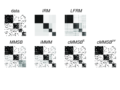
Figure 4: Comparison of the models’ posterior predictive distribution on the training data. The original data is a block diagonal matrix, with some outliers existed as the black points. For the IRM model, its result is composed of rectangular zones. one value is presented in each rectangular. This simplified and “smoothed” version is due to the single membership representation for one node, it can not distinguish the random distributed points. Comparing to this, the LFRM provides a larger amount of values to select from. This enable the model to place different values on one rectangular zone, especially each node is meant to be line-shaped colors, which is in consistent with the one latent features vector for one node representation. However, it still fails to detect the random points. Then comes the MMSB and iMMM in that they have successfully captured the random points. What is more, we find our $\textrm{\emph{cMMSB}}^{\pi}$ and $\textrm{\emph{cMMSB}}^{uv}$ models partition the relational data the best.

4.1.2 Partial correlation - Multiple Copulas in subgroup structure

We also have an additional test case and integrate two Gumbel Copula functions in the modelling. The first 20 nodes are forming a correlated subgroup and share one Copula function, while the other Copula function is applied on the rest of the interactions. The performance on the Full correlation data is shown in Table 3.

While using this model on a Partial correlation dataset, we get the $95\%$ Confidence Interval for both of the recovered $\theta_{1}$ and $\theta_{2}$ displayed in Table 4. We can see that our model can distinguish between the correlated and independent case, where the recovered value of $\theta_{2}$ is much closer to 1.

Table 4: $\theta$’s $95\%$ Confidence Interval

Models	s-cMMSB	s-ciMMM	Ground-truth
$\theta_{1}$	$4.19\mp 0.91$	$3.23\mp 1.22$	3.5
$\theta_{2}$	$1.42\mp 0.23$	$2.39\mp 0.48$	1.0

4.2 Real world datasets’ link prediction

We analyse three real world datasets here: the NIPS Co-authorship dataset, the MIT Reality Mining dataset and the lazega-lawfirm dataset. As the predict ability is one important property of the model, we use a ten-folds cross-validation to complete this task, where we randomly select one out of ten for each node’s link data as test data and the others as training data. The criteria in evaluating this predict ability includes the train error ($0-1$ loss), the test error ($0-1$ loss), the test log likelihood and the AUC (Area Under the roc Curve) score, where detail derivations of these values can refer to the Supplementary Material. Table 5 shows the detail results.

Table 5: Different models’ performance (Mean $\mp$ Standard Deviation) on Real world datasets. From these reported statistics, we can see that our methods ($\textrm{\emph{cMMSB}}^{\pi}$, $\textrm{\emph{cMMSB}}^{uv}$) obtain the best performance in these 3 datasets, amongest all other models.

dataset		Train error	Test error	Test log likelihood	AUC
	IRM	$0.0317\mp 0.0004$	$0.0423\mp 0.0014$	$-135.0467\mp 7.3816$	$0.8901\mp 0.0162$
	LFRM	$0.0482\mp 0.0794$	$0.0239\mp 0.0735$	$-105.2166\mp 179.5505$	$0.9348\mp 0.1667$
NIPS	MMSB	$0.0132\mp 0.0042$	$0.0301\mp 0.0064$	$-86.2134\mp 10.1258$	$0.9524\mp 0.0215$
co-author	iMMM	$\boldsymbol{0.0061\mp 0.0019}$	$0.0253\mp 0.0035$	$-83.4264\mp 9.4293$	$0.9574\mp 0.0155$
	$\textrm{\emph{cMMSB}}^{\pi}$	$0.0066\mp 0.0038$	$\boldsymbol{0.0231\mp 0.0043}$	$-83.4261\mp 9.4280$	$0.9569\mp 0.0159$
	$\textrm{\emph{cMMSB}}^{uv}$	$0.0097\mp 0.0047$	$0.0240\mp 0.0065$	$\boldsymbol{-83.4257\mp 9.4292}$	$\boldsymbol{0.9581\mp 0.0153}$
	IRM	$0.0627\mp 0.0002$	$0.0665\mp 0.0004$	$-133.8037\mp 1.1269$	$0.8261\mp 0.0047$
	LFRM	$0.0397\mp 0.0017$	$0.0629\mp 0.0037$	$-143.6067\mp 10.0592$	$0.8529\mp 0.0179$
MIT	MMSB	$0.0263\mp 0.0105$	$0.0716\mp 0.0043$	$-129.4354\mp 7.6549$	$0.8561\mp 0.0176$
realtiy	iMMM	$0.0297\mp 0.0055$	$0.0625\mp 0.0015$	$-126.7876\mp 3.4774$	$0.8617\mp 0.0124$
	$\textrm{\emph{cMMSB}}^{\pi}$	$\boldsymbol{0.0246\mp 0.0016}$	$0.0489\mp 0.0016$	$-125.3876\mp 3.2689$	$\boldsymbol{0.8794\mp 0.0159}$
	$\textrm{\emph{cMMSB}}^{uv}$	$0.0283\mp 0.0035$	$\boldsymbol{0.0438\mp 0.0015}$	$\boldsymbol{-123.3876\mp 3.1254}$	$0.8738\mp 0.0364$
	IRM	$0.0987\mp 0.0003$	$0.1046\mp 0.0012$	$-201.7912\mp 3.3500$	$0.7056\mp 0.0167$
	LFRM	$0.0566\mp 0.0024$	$0.1051\mp 0.0064$	$-222.5924\mp 16.1985$	$0.8170\mp 0.0197$
Lazega	MMSB	$0.0391\mp 0.0071$	$0.0913\mp 0.0030$	$-212.1256\mp 3.2145$	$0.7989\mp 0.0102$
lawfirm	iMMM	$0.0487\mp 0.0068$	$0.1096\mp 0.0026$	$-202.7148\mp 5.3076$	$0.8074\mp 0.0141$
	$\textrm{\emph{cMMSB}}^{\pi}$	$\boldsymbol{0.0246\mp 0.0050}$	$\boldsymbol{0.1023\mp 0.0056}$	$\boldsymbol{-201.0154\mp 5.2167}$	$\boldsymbol{0.8273\mp 0.0148}$
	$\textrm{\emph{cMMSB}}^{uv}$	$0.0276\mp 0.0043$	$0.1143\mp 0.0019$	$-204.0289\mp 9.5460$	$0.8215\mp 0.0167$

4.2.1 NIPS co-authorship dataset

We use the co-authorship as a relation from the proceeding of the Neural Information Processing Systems (NIPS) conference for the years 2000-2012. As the sparsity of the co-authorship, we observe the authors’ activities in all the 13 years (i.e. regardless of the time factor) and set the relational data being 1 if the two corresponding authors have co-authored for no less than 2 papers, which is to remove the co-authors’ randomness. Further, the author with less than 4 relationships with others are manually eliminated. Thus, a $92\times 92$ symmetric, binary matrix is obtained.

On this dataset, no pre-defined subgroup information is obtained in advance. Thus, we consider it as full-correlation case and use one Gumbel Copula function in modelling all the interactions.

4.2.2 MIT Reality dataset

From the MIT Reality Mining (Eagle & , Sandy), we have used the subjects’ proximity dataset, where weighted links are indicating the average proximity from one subject to another at work. We then“binarize” the data, in which we set the proximity value larger than 10 minutes per day as 1, and 0 otherwise. Therefore, a $94\times 94$ asymmetric, binary matrix is obtained.

The dataset are roughly divided into four groups: Sloan Business School students (Sloan), Lab faculty, senior students with more than 1 year in the lab and junior students. In our experiment, we have only applied the Gumbel Copula function to the Sloan portion of the students to encourage similar mixture membership indicators.

4.2.3 Lazega Law dataset

The lazega-lawfirm dataset (Lazega, 2001) is obtained from a social network study of corporate located in the northeastern part of U.S. in 1988 - 1991. The dataset contains three different types of relations: co-work network, basic advice network and friendship network, among the 71 attorneys, of which the element are labeled as $1$ (exist) or $0$ (absent).

Since no subgroup information is obtained in this dataset, we use one Gumbel Copula function on the whole group and show the corresponding result in Table 5.

5 Conclusions

In this paper, we have proposed a new framework to realistically describe the intra-subgroup correlations in a Mixed-Membership Stochastic Blockmodel. The key to the model is the introduction of the Copula function, which represents the correlation between the pair of membership indicators, while keeping the membership indicators’ marginal distribution invariant. The results show that, using both synthetic and real data, our Copula-incorporated MMSB is effective in learning the community structure and predicting the missing links, when information within a subgroup is known.

In terms of inference, our main contribution is to have obtained an analytical solution to both of the conditional marginal likelihoods to the two indicator variables $(s_{ij},r_{ji})$, given either the indicator distributions $\pi_{i},\pi_{j}$ or the bivariate Copula variables $u_{ij},v_{ij}$.

References

- Airoldi et al. (2008) Airoldi, E.M., Blei, D.M., Fienberg, S.E., and Xing, E.P. Mixed membership stochastic blockmodels. The Journal of Machine Learning Research, 9:1981–2014, 2008.
- Blei et al. (2010) Blei, David M., Griffiths, Thomas L., and Jordan, Michael I. The nested chinese restaurant process and bayesian nonparametric inference of topic hierarchies. Journal of ACM, 57(2):7:1–7:30, February 2010. ISSN 0004-5411. doi: 10.1145/1667053.1667056.
- Chen et al. (2013) Chen, C., Rao, V. A., Buntine, W., and Teh, Y. W. Dependent normalized random measures. In Proceedings of the International Conference on Machine Learning, 2013.
- Eagle & (Sandy) Eagle, Nathan and (Sandy) Pentland, Alex. Reality mining: sensing complex social systems. Personal Ubiquitous Comput., 10(4):255–268, 2006. ISSN 1617-4909.
- Fortunato (2010) Fortunato, S. Community detection in graphs. Physics Reports, 486(3):75–174, 2010.
- Foti et al. (2012) Foti, Nicholas J., Futoma, Joseph D., Rockmore, Daniel N., and Williamson, Sinead. A unifying representation for a class of dependent random measures. CoRR, abs/1211.4753, 2012.
- Girvan & Newman (2002) Girvan, M. and Newman, M.E.J. Community structure in social and biological networks. Proceedings of the National Academy of Sciences, 99(12):7821–7826, 2002.
- Griffiths & Ghahramani (2005) Griffiths, Thomas L. and Ghahramani, Zoubin. Infinite latent feature models and the indian buffet process. In Advances in Neural Information Processing Systems 18, pp. 475–482. MIT Press, 2005.
- Griffiths & Ghahramani (2011) Griffiths, Thomas L and Ghahramani, Zoubin. The indian buffet process: An introduction and review. Journal of Machine Learning Research, 12:1185–1224, 2011.
- Ho et al. (2012) Ho, Qirong, Parikh, Ankur P., and Xing, Eric P. A multiscale community blockmodel for network exploration. Journal of the American Statistical Association, 107(499):916–934, 2012. doi: 10.1080/01621459.2012.682530.
- Hoff (2005) Hoff, Peter D. Bilinear mixed-effects models for dyadic data. Journal of the american Statistical association, 100(469):286–295, 2005.
- Hoff et al. (2002) Hoff, Peter D, Raftery, Adrian E, and Handcock, Mark S. Latent space approaches to social network analysis. Journal of the american Statistical association, 97(460):1090–1098, 2002.
- Ishiguro et al. (2010) Ishiguro, Katsuhiko, Iwata, Tomoharu, Ueda, Naonori, and Tenenbaum, Joshua B. Dynamic infinite relational model for time-varying relational data analysis. In NIPS, pp. 919–927. Curran Associates, Inc., 2010.
- Kemp et al. (2006) Kemp, C., Tenenbaum, J.B., Griffiths, T.L., Yamada, T., and Ueda, N. Learning systems of concepts with an infinite relational model. In Proceedings of the national conference on artificial intelligence, volume 21, pp. 381. Menlo Park, CA; Cambridge, MA; London; AAAI Press; MIT Press; 1999, 2006.
- Kim et al. (2012) Kim, D.I., Hughes, M., and Sudderth, E. The nonparametric metadata dependent relational model. In Proceedings of the 29th Annual International Conference on Machine Learning. ACM, 2012.
- Koutsourelakis & Eliassi-Rad (2008) Koutsourelakis, P.S. and Eliassi-Rad, T. Finding mixed-memberships in social networks. In Proceedings of the 2008 AAAI spring symposium on social information processing, 2008.
- Lazega (2001) Lazega, E. The collegial phenomenon: The social mechanisms of cooperation among peers in a corporate law partnership. 2001.
- Lin & Fisher (2012) Lin, Dahua and Fisher, John. Coupling nonparametric mixtures via latent dirichlet processes. In Advances in Neural Information Processing Systems 25, pp. 55–63, 2012.
- Lin et al. (2010) Lin, Dahua, Grimson, Eric, and Fisher III, John W. Construction of dependent dirichlet processes based on poisson processes. Neural Information Processing Systems Foundation (NIPS), 2010.
- Liu (1994) Liu, Jun S. The collapsed gibbs sampler in bayesian computations with applications to a gene regulation problem. Journal of the American Statistical Association, 89(427):958–966, 1994.
- MacEachern (1999) MacEachern, Steven N. Dependent nonparametric processes. In ASA proceedings of the section on bayesian statistical science, pp. 50–55. American Statistical Association, pp. 50–55, Alexandria, VA, 1999.
- McNeil & Nešlehová (2009) McNeil, Alexander J and Nešlehová, Johanna. Multivariate archimedean copulas, d-monotone functions and -norm symmetric distributions. The Annals of Statistics, pp. 3059–3097, 2009.
- Miller et al. (2009) Miller, Kurt, Griffiths, Thomas, and Jordan, Michael. Nonparametric latent feature models for link prediction. Advances in neural information processing systems, 22:1276–1284, 2009.
- Nelsen (2006) Nelsen, R.B. An introduction to copulas. Springer, 2006.
- Newman & Girvan (2004) Newman, M.E.J. and Girvan, M. Finding and evaluating community structure in networks. Physical review E, 69(2):026113, 2004.
- Nowicki & Snijders (2001) Nowicki, Krzysztof and Snijders, Tom A. B. Estimation and prediction for stochastic blockstructures. Journal of the American Statistical Association, 96(455):1077–1087, 2001.
- Palla et al. (2012) Palla, Konstantina, Knowles, David A., and Ghahramani, Zoubin. An infinite latent attribute model for network data. In Proceedings of the 29th International Conference on Machine Learning, ICML 2012. Edinburgh, Scotland, GB, July 2012.
- Schwarz (1978) Schwarz, Gideon. Estimating the dimension of a model. The annals of statistics, 6(2):461–464, 1978.
- Sethuraman (1991) Sethuraman, J. A constructive definition of dirichlet priors. Technical report, DTIC Document, 1991.
- Tang & Liu (2010) Tang, Lei and Liu, Huan. Community detection and mining in social media. Synthesis Lectures on Data Mining and Knowledge Discovery, 2(1):1–137, 2010.
- Teh et al. (2006) Teh, Y.W., Jordan, M.I., Beal, M.J., and Blei, D.M. Hierarchical dirichlet processes. Journal of the American Statistical Association, 101(476):1566–1581, 2006.
- Xing et al. (2010) Xing, E.P., Fu, W., and Song, L. A state-space mixed membership blockmodel for dynamic network tomography. The Annals of Applied Statistics, 4(2):535–566, 2010.
- Yang et al. (2011) Yang, Tianbao, Chi, Yun, Zhu, Shenghuo, Gong, Yihong, and Jin, Rong. Detecting communities and their evolutions in dynamic social networks - a bayesian approach. Machine Learning, 82(2):157–189, 2011.