Mean–Variance and Expected Utility: The Borch Paradox

Abstract

The model of rational decision-making in most of economics and statistics is expected utility theory (EU) axiomatised by von Neumann and Morgenstern, Savage and others. This is less the case, however, in financial economics and mathematical finance, where investment decisions are commonly based on the methods of mean–variance (MV) introduced in the 1950s by Markowitz. Under the MV framework, each available investment opportunity (“asset”) or portfolio is represented in just two dimensions by the ex ante mean and standard deviation $(\mu,\sigma)$ of the financial return anticipated from that investment. Utility adherents consider that in general MV methods are logically incoherent. Most famously, Norwegian insurance theorist Borch presented a proof suggesting that two-dimensional MV indifference curves cannot represent the preferences of a rational investor (he claimed that MV indifference curves “do not exist”). This is known as Borch’s paradox and gave rise to an important but generally little-known philosophical literature relating MV to EU. We examine the main early contributions to this literature, focussing on Borch’s logic and the arguments by which it has been set aside.

and

There is no inevitable connection between the validity of the expected utility maxim and the validity of portfolio analysis based on, say, expected return and variance (Markowitz, 1959, page 209).

1 Introduction

This paper looks back at a little-known but highly interesting chapter in the history of business decision-making (call it “investment”) under uncertainty. In a once fêted but now rarely mentioned paper, titled politely A Note on Uncertainty and Indifference Curves, the Norwegian insurance theorist and economist Karl Borch (1969) argued that the mean–variance theory of investment, invented and popularized by Markowitz (1952, 1959), is logically absurd. In this delightfully provocative note, Borch (1969) proved, he claimed, that it is impossible to draw indifference curves in the mean–variance $(\mu,\sigma^{2})$ or mean–standard deviation $(\mu,\sigma)$ plane. The same proof appears in at least two other works by Borch (1973, 1974), who concluded that mean–variance is an interesting but not serious alternative to expected utility:

$\ldots$ I shall continue to use mean–variance analysis in teaching, but I shall warn students that such analysis must not be taken seriously and applied in practice (Borch (1974), page 430).

The proof presented by Borch (pronounced“Bork”) became known to theorists as “Borch’s paradox”. While of much interest theoretically, the academic discussion that stemmed from Borch’s work had virtually no impact on the practice of finance. To the contrary, mean–variance (MV) analysis, for which Markowitz later won a Nobel Prize in Economic Sciences, has become by far the most recognized decision framework in the practice of business decision-making, including especially capital budgeting (e.g., whether to build a new factory), investment management (e.g., whether to increase the weight of oil stocks in a pension fund) and corporate financial valuation (e.g., whether a firm is worth its current value on the stock market). Each of these common applications is built implicitly on MV, and explicitly on the so-called “capital asset pricing model” (CAPM) that arose as a corollary from the MV foundations set out by Markowitz.

Although business applications of MV portfolio theory and the CAPM are commonplace, and effectively the industry standard (witness any modern textbook in financial economics), proponents of this decision framework remain conscious that the proven philosophical foundations of decision analysis under uncertainty remain the axioms and theorems of expected utility theory (EU), formalized by Von Neumann and Morgenstern (1953) and Savage (1954). Utility theory, or more specifically the maximization of subjective expected utility satisfying the von Neumann–Morgenstern or similar axioms, remains the hallmark of rationality in economics and statistical decision analysis (e.g., DeGroot (1970); Bernardo and Smith (1994); Pratt, Raiffa and Schlaifer (1995); Lengwiler (2004); Eeckhoudt, Gollier and Schlesinger (2005)). As a mark of respect for this intellectual legacy, Markowitz (1991) devoted his 1990 Nobel Lecture to an empirical comparison of his MV methods of portfolio selection with a model based on EU theory. Authoritative recognition also goes the other way. In its second edition, one of the standard references on neoclassical decision theory, Pratt, Raiffa and Schlaifer (1995) contains an elegant exposition of the MV investment framework, albeit without reconciliation with other explicitly EU parts of the book. Completing the circle, Markowitz (2006) and Rubinstein (2006a) have lately pointed to an early paper in Italian, authored by de Finetti (1940), the most revered of all subjective probability theorists, as having been first to express a formal model of decision-making within a MV framework. Two further expositions concentrated on de Finetti’s previously little-known anticipation of Markowitz are Barone (2008) and Pressacco and Serafini (2007).

Our primary purpose is to examine the historical literature surrounding Borch’s paradox. To assist readers who are not familiar with this branch of applied statistical literature, we first recount the basic elements of investment decision-making under the two competing conceptual frameworks, expected utility and mean–variance. We then consider how MV can be justified on axiomatic foundations, in the face of critics such as Borch, and by comparison with EU theory generally. Finally, to better understand the practical appeal of MV methods, and why finance theory so readily adopted the language of MV over EU, we introduce the capital asset pricing model (CAPM) and observe how such a theoretically insightful model arose almost automatically once decisions were depicted in terms of MV rather than EU.

2 Expected Utility Theory

A decision is a choice between some (usually strict) subset of all of the available “lotteries,” “assets,” “investments” (these terms are synonyms)—and all feasible weighted portfolios thereof. Each such uncertain prospect reduces to a probability distribution over a domain of possible payoffs. Decision-making is therefore boiled down to a choice between different possible probability distributions of returns.

Von Neumann and Morgenstern (1953) proposed an axiomatic theory of how to decide between known probability distributions (of payoffs). In brief, they proved deductively that if decision-making is logical in the sense that it obeys certain specified basic axioms of coherence or rationality, then implicitly the decision-maker must act as if her objective is to maximize expected utility $E[u(x)]=\int_{x}f(x)u(x)$, where $u(x)$ is a real-valued function representing the utility obtained from certain wealth or payoff $x$, and $f(x)$ is the probability density function of $x$. The decision rule of maximizing $E[u(x)]$, taken in conjunction with some plausible looking utility function such as Bernoulli’s $u(x)=\log(x)$, is often treated as itself axiomatic. More correctly, the extra-intuitive appeal of the EU decision rule is that rather than being just another plausible looking but arbitrary objective function, it is a theorem deduced from a small number of far more elementary assumptions concerning what constitutes rational human preferences.

There are five essential axioms of expected utility: (i) Completeness. All lotteries $A$ and $B$ can be ranked relative to one another, $A\succ B$, $A\prec B$ or $A\sim B$, where $\sim$ indicates indifference. (ii) Transitivity. If $A\succeq B$ and $B\succeq C$, then $A\succeq C$. (iii) Continuity. If $A\succeq B\succeq C$, there exists some probability $\alpha\in[0,1]$ such that $B\sim\alpha A+(1-\alpha)C$, meaning that $B$ is indifferent to a compound lottery that returns lottery $A$ with probability $\alpha$ and lottery $C$ with probability $(1-\alpha)$. (iv) Independence. Indifference $A\sim B$ between lotteries $A$ and $B$ implies indifference between compound lottery $\alpha A+(1-\alpha)C$ and compound lottery $\alpha B+(1-\alpha)C$. Similarly, $A\succ B$ implies $\alpha A+(1-\alpha)C\succ\alpha B+(1-\alpha)C$, for $\alpha>0$. (v) Dominance. Let $C_{1}$ be the compound lottery $\alpha_{1}A+(1-\alpha_{1})B$ and let $C_{2}$ be the compound lottery $\alpha_{2}A+(1-\alpha_{2})B$. If $A\succ B$, then $C_{1}\succ C_{2}$ if and only if $\alpha_{1}>\alpha_{2}$.

For further interpretation of these axioms andproof of how they lead to the von Neumann and Morgenstern EU decision rule, see Pennacchi (2008), pages 4–11. Similar expositions are found in many textbooks both in economics and statistics. See, for example, Ingersoll (1987), pages 30–44, Huang and Litzenberger (1988), pages 1–11, and Levy (2012), pages 25–30. In brief, by assuming the primitive preference relationships (i)–(v), it is shown that lottery $A$ is preferred to lottery $B$ if and only if the expected utility of lottery $A$ exceeds the expected utility of lottery $B$. Expected utility $E[u(x)]$ is therefore the proven measure by which to rank uncertain investments.

The usual assumption in economics is that decision-makers are risk averse. This means that they have positive but diminishing marginal utility for money, and hence $u(x)$ is increasing and concave. A risk averse decision-maker will not accept any lottery with an expected money value of zero (or less). Actuarially fair bets are thus unacceptable. Before accepting a bet to win or lose some fixed sum $c$, a risk averse agent requires that the probability of winning exceeds 0.5 by some premium. The amount of this premium depends on the local concavity of $u(x)$ or on how fast the marginal utility of money is diminishing in the region of wealth $x_{0}\pm c$, where $x_{0}$ is her starting wealth. Technically, the Pratt–Arrow measure of local absolute risk aversion $-u^{\prime\prime}(x)/u^{\prime}(x)$ captures the degree of concavity of $u$ or the rate at which marginal utility is decreasing at wealth $x$.

3 Mean–Variance Theory

The following quick summary of MV owes much to Liu (2004). The one-period return on an investment over period $t$ is defined as $(p_{t}+d)/p_{t-1}$, where $p_{t}$ is the time $t$ asset price and $d$ is the income (dividend) drawn from the asset in period $t$. This definition has the advantage that the returns measure is always positive.

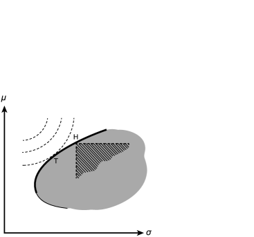
Figure 1: Graphical presentation of $\operatorname{MV}(\sigma,\mu)$ analysis.

Imagine a set of available investments or “assets”. These can be combined into arbitrarily weighted portfolios (e.g., the investor might form a 2:1 weighted portfolio of assets A and B, where two-thirds of her money is invested in A and one-third in B). The available assets and their linearly weighted portfolios form an opportunity set of investments. Each possible asset or portfolio presents a compromise between mean return $\mu$ and variance $\sigma^{2}$. Each such MV pair is reduced following Markowitz and finance convention to its parameters $(\sigma,\mu)$. The opportunity set is then a region of feasible $(\sigma,\mu)$ pairs. This region is depicted in its characteristic shape by the bullet-like shaded area in Figure 1. The investor is generally risk averse and thus prefers portfolios with higher mean return $\mu$ and lower “risk” (standard deviation) $\sigma$. The opportunity set is reduced therefore to just those portfolios on the thick black arc called the “efficient frontier”. Each asset portfolio on the efficient frontier dominates all assets and portfolios to its southeast, because these have both lower $\mu$ and higher $\sigma$. For example, asset $(\sigma,\mu)$-pair $H$ dominates all assets and portfolios in the hatched region.

To choose between all efficient portfolios, the investor forms a family of MV indifference curves. These are understood as equivalue curves defined by some indifference function $V(\sigma,\mu)$. Each such curve shows the locus of $(\sigma,\mu)$ points for which $V(\sigma,\mu)$ is held constant. A typical looking family of indifference curves is shown by the dotted lines in Figure 1. These curves are drawn convex downwards on the basis that, for assets known only by their MV parameters $(\sigma,\mu)$, the risk averse investor requires marginally greater compensation in $\mu$ for each further increment in risk $\sigma$ (see Meyer (1987), for related proofs). Since risk averse investors prefer lower $\sigma$ for fixed $\mu$, higher (more northwesterly) indifference curves represent greater expected utility to the investor. Having established both the efficient frontier and an indifference function $V(\sigma,\mu)$, the unique MV-optimal investment in risky assets is located at the point of tangency $T$ between the decision-maker’s own $V(\sigma,\mu)$ and the exogenous efficient frontier.

4 Borch’s Paradox

Borch (1969), pages 2 and 3, presented a proof based on assets with two-point distributions that revealed (he claimed) that it is impossible to draw indifference curves in the mean–variance $(\mu,\sigma^{2})$ or mean–standard deviation $(\mu,\sigma)$ plane. Borch repeated this same proof in 1973 and 1974, and wrote openly of his frustration that it was not more widely acknowledged by theorists developing portfolio optimization methods:

I have on several occasions (1969) and (1974) tried to warn against the uncritical use of mean–variance analysis. It was probably too much to expect that these warnings should have much effect (Borch (1978), page 181).

The Borch paradox goes as follows. First, assume that two assets (payoff distributions) with parameters $(\mu_{1},\sigma_{1}^{2})$ and $(\mu_{2},\sigma_{2}^{2})$ are regarded, on the basis of those parameters alone, as indifferent (i.e., of equal subjective merit). Now imagine two hypothetical assets constructed simply as two-point distributions. Asset 1 produces payoff $y_{1}$ with probability $p$ and payoff $x$ with probability $(1-p)$. Asset 2 produces payoff $y_{2}$ with probability $p$ and payoff $x$ with probability $(1-p)$. By common sense or some very basic axiom like the “sure thing” principle raised by Savage (Borch cites Allais’ concept of “preference absolue”), these two assets are indifferent if and only if $y_{1}=y_{2}$ $(p>0)$.

Now, suppose that the constants $x$, $p$, $y_{1}$ and $y_{2}$ take values

$$x = \frac{\sigma_{1}\mu_{2}-\sigma_{2}\mu_{1}}{\sigma_{1}-\sigma_{2}},$$ (1)

$$p = \frac{(\mu_{1}-\mu_{2})^{2}}{(\mu_{1}-\mu_{2})^{2}+(\sigma_{1}-\sigma_{2})^{2}},$$ (2)

$$y_{1} = \mu_{1}+\sigma_{1}\frac{(\sigma_{1}-\sigma_{2})}{(\mu_{1}-\mu_{2})},$$ (3)

$$y_{2} = \mu_{2}+\sigma_{2}\frac{(\sigma_{1}-\sigma_{2})}{(\mu_{1}-\mu_{2})}.$$ (4)

Borch did not make any mention of where these equations come from or what they assume, except to say that it is easy to verify that the implied values of the mean and variance parameters of the two assets are, respectively, $(\mu_{1},\sigma_{1}^{2})$ and $(\mu_{2},\sigma_{2}^{2})$, thus matching assets 1 and 2 (this is indeed easily verified).

The final step in Borch’s proof holds that because the two assets can be of equal merit only if $y_{1}=y_{2}$, the indifference condition $\mbox{(\ref{equ3})}=\mbox{(\ref{equ4})}$ is

$$\mu_{1}+\sigma_{1}\frac{(\sigma_{1}-\sigma_{2})}{(\mu_{1}-\mu_{2})}=\mu_{2}+\sigma_{2}\frac{(\sigma_{1}-\sigma_{2})}{(\mu_{1}-\mu_{2})},$$

implying that $(\mu_{1}-\mu_{2})^{2}+(\sigma_{1}-\sigma_{2})^{2}=0$ and, hence, indifference requires that $\mu_{1}=\mu_{2}$ and $\sigma_{1}=\sigma_{2}.$ According to Borch’s interpretation of this result, any supposed indifference between two arbitrary mean–variance pairs is impossible, unless of course they are the same. Mean–variance indifference curves are thus merely points rather than curves, or, in Borch’s [(1969), page 3] own words, “it is impossible to draw indifference curves in the E–S-plane” (E and S denote the mean and standard deviation).

In answer to any suspicion raised by their nonexplanation, there is nothing contrived about the four equations used by Borch to define the constants $x$, $p$, $y_{1}$ and $y_{2}$ in his proof. Rather, these can be derived by writing the standard equations for the means and standard deviations, $\mu_{1}$, $\mu_{2}$, $\sigma_{1}$ and $\sigma_{2}$, of the two Borch two-point assets in terms of $x$, $p$, $y_{1}$ and $y_{2}$, and then solving these four equations simultaneously to get general expressions for all four constants in terms of the specified means and standard deviations. It follows, therefore, that the four Borch equations, numbered (1)–(4) above, are not merely sufficient conditions to produce the specified mean–variance parameters $(\mu_{1},\sigma_{1}^{2})$ and $(\mu_{2},\sigma_{2}^{2})$. Rather, they follow necessarily from those specified parameter values as one of two possible sets of solutions. The second set of solutions, which Borch did not raise but could have employed to the same effect, is as follows:

$$x = \frac{\sigma_{1}\mu_{2}+\sigma_{2}\mu_{1}}{\sigma_{1}+\sigma_{2}},$$

$$p = \frac{(\mu_{1}-\mu_{2})^{2}}{(\mu_{1}-\mu_{2})^{2}+(\sigma_{1}+\sigma_{2})^{2}},$$

$$y_{1} = \mu_{1}+\sigma_{1}\frac{(\sigma_{1}+\sigma_{2})}{(\mu_{1}-\mu_{2})},$$

$$y_{2} = \mu_{2}+\sigma_{2}\frac{(\sigma_{1}+\sigma_{2})}{(\mu_{1}-\mu_{2})}.$$

4.1 Our Interpretation of Borch

Borch interprets his paradox to say that mean–variance indifference curves cannot exist. This is too strong, as will be seen in the sections below. More reasonable interpretations of Borch’s proof are as follows.

Interpretation 1: Suppose that a decision-maker is adamant that he is indifferent between any two assets with mean–variance characteristics $(\mu_{1},\sigma_{1}^{2})$ and $(\mu_{2},\sigma_{2}^{2})$, where $(\mu_{1},\sigma_{1}^{2})\neq(\mu_{2},\sigma_{2}^{2})$. It is possible to construct two-point assets with these very characteristics between which no one can reasonably be indifferent [these can be constructed by Borch’s equations (1)–(4), or equally well with the second possible set of solutions noted above].

This possibility does not imply that there are no possible assets with parameters $(\mu_{1},\sigma_{1}^{2})$ and $(\mu_{2},\sigma_{2}^{2})$ that are rationally (to someone) indifferent. Rather, it shows that the decision-maker cannot be indifferent between all imaginable pairs of assets with these parameters.

Interpretation 2: If we limit consideration to only the particular subclass of two-point assets constructed by Borch, there exists no pair of assets with $(\mu_{1},\sigma_{1}^{2})\neq(\mu_{2},\sigma_{2}^{2})$ between which anyone might reasonably be indifferent. Rather, whenever $(\mu_{1},\sigma_{1}^{2})\neq(\mu_{2},\sigma_{2}^{2})$, the two assets (having $x$ and $p$ in common) necessarily differ in that $y_{1}\neq y_{2}$, which of itself means that they cannot be indifferent.

4.2 Numerical Illustration

Here we exemplify Interpretation 1 numerically. Imagine that the subject of the experiment feels that he is indifferent between any two assets with parameters $(\mu_{1},\sigma_{1}^{2})=(10,225)$ and $(\mu_{2},\sigma_{2}^{2})=(20,625)$.Such subjective indifference would typically require that the security with the bigger mean has the bigger variance, but that practicality is not necessary in Borch’s demonstration. Now consider two comparable lottery tickets, ticket A and ticket B. Ticket A pays $25$ with probability $p=0.5$ and $-5$ with probability $(1-p)$. Similarly, ticket B pays $45$ with probability $p=0.5$ and $-5$ with probability $(1-p)$. The mean–variance parameters of these two lotteries are $(10,225)$ and $(20,625)$, respectively. Yet contrary to any thought that two assets with these parameters are indifferent, ticket B is obviously preferred because it has the same probability of winning as ticket A, and the same payoff if it loses, but pays 45 instead of 25 when it wins. Borch saw this apparent contradiction as proof that the decision-maker cannot logically be indifferent between two investments by reference only to their means and variances.

5 Baron’s Rebuttal of Borch

Borch’s paradox is well known to those economic theorists mindful of foundations and interested in the history of mean–variance, yet is largely unknown elsewhere and goes unmentioned in standard finance and financial economics texts, even in highly sophisticated works such as Ingersoll (1987), Cochrane (2001), Barucci (2003), Lengwiler (2004) and Pennacchi (2008) that deal with the connections between mean–variance models and expected utility theory. Neither is Borch mentioned in the very thorough historical annotated bibliography of Rubinstein (2006b). This omission is justified perhaps by the findings of a similarly important but now rarely mentioned paper by Baron (1977).

Baron rebuts Borch’s paradox in two steps. First comes the proposition that decision-making based on just the two parameters, mean and variance, implies an underlying quadratic utility function. The same argument arises in Hanoch and Levy [(1970), page 182] and Sarnat [(1974), page 687] who both note that quadratic (second order polynomial) utility is the only form of mathematical utility function for which expected utility reduces to a function of just the first two moments of the payoff distribution. Specifically, for risk-averse quadratic utility $u(x)=2ax-x^{2}$, the expected utility is $E[u(x)]=2a\mu-(\mu^{2}+\sigma^{2})$. Similarly, see the derivation by Liu (2004), page 233.

The presumption that MV necessarily implies quadratic utility traces to Markowitz [(1959), page 288] and also Mossin (1973), pages 26 and 27. Hanoch and Levy [(1970), page 182] hold that “rejection of quadratic utility implies the rejection of any analysis based on the expected utility maxim”, which is indirectly saying that the only unconditional way of hanging onto EU while applying MV is to adopt quadratic utility. Johnstone and Lindley (2011) have more recently given an elementary proof revealing that, in the absence of any further premise, MV necessitates quadratic utility.

Having concluded that Borch’s proposed subjective value function can arise from only a quadratic utility function, Baron’s second step is to show that one of the asset pairs in Borch’s counterexample, $(\mu_{1},\sigma_{1}^{2})$ and $(\mu_{2},\sigma_{2}^{2})$, must involve a potential payoff in the domain where quadratic utility is decreasing with money. This finding is easy to understand intuitively. The two Borch assets are identical except that $y_{1}\neq y_{2}$ and, hence, the asset with the lower $y$ (e.g., asset 1 if $y_{1}<y_{2}$) can only be as good in someone’s mind as the asset with the higher $y$ if that higher $y$ is in the domain where money has negative marginal utility, thus allowing $y_{1}$ and $y_{2}$ to have the same utility $u(y_{i})$.

The net effect of Baron’s argument can be summarized as follows:

[(iii)]

Borch’s paradox proves only that for any two mean–variance pairs, $(\mu_{1},\sigma_{1}^{2})$ and $(\mu_{2},\sigma_{2}^{2})$, a rational decision-maker cannot be indifferent between all pairs of assets with the specified parameters. Indeed, precisely as Borch revealed, there are easily definable assets with such characteristics which are obviously not indifferent.

If the decision-maker has quadratic utility, EU can be written as a function of mean and variance alone and, hence, $(\sigma,\mu)$ indifference curves do exist. It is necessary, however, to constrain the class of assets under consideration so as to exclude any asset with one (or more than one) potential payoff in the region where utility decreases with money. Negative marginal utility for some $x$ is a well-known limitation of quadratic utility, and is bound to produce irrational or incoherent decisions even under EU if the admissible asset class is not suitably restricted.

If assets with possible payoffs in the domain where quadratic utility decreases with money (i.e., where the last increment of payoff brings a reduction in utility) are excluded a priori from consideration, as if they cannot exist, then the class of counterexamples constructed by Borch (and illustrated numerically above) no longer exists.

Another somewhat forgotten finding should bementioned here. Taking MV as a representation of quadratic utility, and constraining all possible payoffs into the domain where quadratic utility is increasing, Levy and Sarnat [(1972), pages 387 and 388] proved that one MV asset pair $(\mu_{1},\sigma_{1}^{2})$ has higher utility than another $(\mu_{2},\sigma_{2}^{2})$, with $\mu_{1}>\mu_{2}$, if and only if $(\mu_{1}-\mu_{2})^{2}-(\sigma_{1}-\sigma_{2})^{2}>0.$ This is a stronger condition than the usual definition of dominance (i.e., $\mu_{1}\geq\mu_{2}$ and $\sigma_{1}<\sigma_{2}$ or $\mu_{1}>\mu_{2}$ and $\sigma_{1}\leq\sigma_{2}$) and is therefore more “efficient” in the sense that it reduces the class of possible investments to a smaller number.

6 Buridan’s Axiom and Mean–Variance

We now summarize our own disproof of generalized mean–variance analysis, very much in spirit with Borch, and then side with Baron by considering possible theoretical and practical restrictions on the admissible asset class that allow a partial reconciliation between the two ways of decision-making.

Following a convention in finance dating to Markowitz’s original exposition of the mean–variance framework, our analysis is set out in terms of the standard deviation $\sigma$ rather than variance $\sigma^{2}$. Adhering to another well-entrenched custom in the finance literature, we work with $\sigma$ as abscissa and $\mu$ as ordinate.

6.1 Decision Axioms in Terms of $(\sigma,\mu)$

Suppose there exists a value function $g(\sigma,\mu)$ that captures the merit or goodness of a $(\sigma,\mu)$-asset such that larger $g$ implies greater value. Indifference between two assets $(\sigma_{1},\mu_{1})$ and $(\sigma_{2},\mu_{2})$ means that $g(\sigma_{1},\mu_{1})=g(\sigma_{2},\mu_{2})$. It is not necessary to be explicit about the form of $g$.

Continuity-monotonicity-finiteness (CMF) axiom. The merit function $g(\sigma,\mu)$ is continuous, strictly increasing in $\mu$ for every $\sigma$, and strictly decreasing in $\sigma$ for every $\mu$. These properties hold throughout the $(\sigma,\mu)$ half-plane, $\sigma\geq 0$. Continuity implies that there is no abrupt change in merit as either $\sigma$ or $\mu$ changes slightly. Strict monotonicity reflects the merit, either positive or negative, of any change in $\mu$ or $\sigma$, however small. Finiteness requires that any finite increase in $\sigma$ can be offset by a sufficiently large finite increase in $\mu$. The existence of such a merit function implies transitivity, meaning that if asset X is preferred to Y, and Y to Z, then X is preferred to Z (and likewise when preference is replaced by indifference).

Buridan’s axiom. If a decision-maker is indifferent between two assets $i=1$ and $i=2$, then he must also be indifferent between either asset and a probability-mixture asset that yields (the same payoff as) $i=1$ with probability $\alpha$ and (the same payoff as) $i=2$ with probability $(1-\alpha)$, where $\alpha$ takes any value $\alpha\in[0,1]$. Thus, according to the merit function $g(\sigma,\mu)$, indifference $g(\sigma_{1},\mu_{1})=g(\sigma_{2},\mu_{2})$ implies $g(\sigma_{1},\mu_{1})=g(\sigma_{2},\mu_{2})=g(\sigma_{\alpha},\mu_{\alpha})$, where $\sigma_{\alpha}$ and $\mu_{\alpha}$ represent the mean and standard deviation of an $\alpha$-mixture of the two indifferent “pure” assets (for any probability $\alpha$). Note that Buridan’s axiom is a simple corollary of the independence axiom in EU.

The question now is whether a decision analysis constructed solely in terms of $(\sigma,\mu)$ can coexist with these two axioms. Consider an asset with $\sigma=0$, known in finance as a “risk-free” asset and approximated by government bonds. Let this asset return $\mu_{0}$, as represented by the point A in Figure 2 with coordinates $(0,\mu_{0})$. Now take any fixed $\sigma_{1}>0$ and points $(\sigma_{1},\mu)$ for all $\mu>0$. These represent risky assets, among which asset B with coordinates $(\sigma_{1},\mu_{0})$ is inferior to (has lower “merit” than) asset A because it has $\mu=\mu_{0}$ but greater $\sigma$. As $\mu$ increases from $\mu_{0}$, the assets on $\sigma=\sigma_{1}$ increase in merit, such that at some point C, with coordinates $(\sigma_{1},\mu_{1})$, the higher return $\mu_{1}=\mu_{0}$ is just sufficient to compensate for the associated risk $\sigma_{1}$, leaving the decision-maker indifferent between C and A. The existence of $\mu_{1}$ is guaranteed by the CMF axiom.

Figure 2: Axiomatic decision analysis in terms of $(\sigma,\mu)$.

Assuming that the decision-maker is indifferent between asset A at $(\sigma_{0}=0,\mu_{0})$ and asset C at $(\sigma_{1},\break\mu_{1})$, Buridan’s axiom dictates that this indifference extends to a randomized mixture of A and C, where A is selected with chance $\alpha$. The payoff $x$ from such an $\alpha$-mixture asset of any pair $(\sigma_{0},\mu_{0})$ and $(\sigma_{1},\mu_{1})$ has expectations

$$\mu=E(x)=\alpha\mu_{0}+(1-\alpha)\mu_{1}$$ (5)

and

$$E\bigl{(}x^{2}\bigr{)} = \alpha\bigl{(}\mu_{0}^{2}+\sigma_{0}^{2}\bigr{)}+(1-\alpha)\bigl{(}\mu_{1}^{2}+\sigma_{1}^{2}\bigr{)}$$

$$= \alpha\mu_{0}^{2}+(1-\alpha)\bigl{(}\mu_{1}^{2}+\sigma_{1}^{2}\bigr{)}\quad(\sigma_{0}=0).$$

Since var$(x)=E(x^{2})-E(x)^{2}$, simple algebra gives

$$\sigma^{2} = \operatorname{var}(x)$$

$$= \alpha\sigma_{0}^{2}+(1-\alpha)\sigma_{1}^{2}+\alpha(1-\alpha)(\mu_{1}-\mu_{0})^{2}$$

$$= (1-\alpha)\sigma_{1}^{2}+\alpha(1-\alpha)(\mu_{1}-\mu_{0})^{2}\quad(\sigma_{0}=0)$$

in the same way as found by Baron (1977), page 1685. Note that equations (5) and (6.1) hold generally for fixed $\alpha$ and do not require $\sigma_{0}=0$ or independent payoffs.

Equation (5) says that the mean of the mixture asset is a weighted average of $\mu_{0}$ and $\mu_{1}$. Equation (6.1) says that the variance does not have this property; its value is not simply $\alpha\sigma_{0}^{2}+(1-\alpha)\sigma_{1}^{2}$, but is inflated by an extra term, $\alpha(1-\alpha)(\mu_{1}-\mu_{0})^{2}$, determined by the difference between the two underlying means.

To satisfy Buridan, the decision-maker must be indifferent between the two original assets, A and C, and a set of $\alpha$-mixture assets with parameters $(\sigma_{\alpha},\mu_{\alpha})$ given by (5) and (6.1), with $\alpha$ taking values between 0 and 1. These assets lie on a curve connecting A and C. The equation of this curve (which is the indifference curve implied by the Buridan axiom) is found by solving (5) and (6.1) so as to eliminate $\alpha$, giving

$$\sigma^{2}+\bigl{[}\mu-(\rho_{0}+\mu_{0})\bigr{]}^{2}=\rho_{0}^{2},$$ (7)

where $\rho_{0}={\frac{1}{2}}[\sigma_{1}^{2}/(\mu_{1}-\mu_{0})+(\mu_{1}-\mu_{0})]$.

Note that the Buridan-based indifference curve (7) has the form of a circle in the $(\sigma,\mu)$ plane, with centre at $(0,\mu_{0}+\rho_{0})$ and radius $\rho_{0}$ (hence the notation). To be sensible, no two indifference circles can intersect.

Although (7) represents a full circle, further considerations reveal that only part of this circle constitutes a sensible indifference curve. The part of (7) with $\sigma<0$ may be ignored because negative $\sigma$ does not exist. The quarter circle DE can also be ignored, because any point on (7) between D and E is better than D. It has smaller $\sigma$ and larger $\mu$ and hence must be preferred under the continuity axiom. This leaves as a plausible indifference curve only the quarter circle AD, of which only the part between A and C is justified so far, having been derived from the Buridan axiom.

It remains, therefore, to examine the arc between C and D, for which $\sigma_{1}<\sigma\leq\rho_{0}$. Let $\sigma^{\ast}$ fall in this interval, and consider all assets $(\sigma^{\ast},\mu)$ on the vertical line through $\sigma=\sigma^{\ast}$. Just as for $\sigma_{1}$, the CMF axiom requires that there is an asset F on this line with sufficiently high $\mu$ to make the decision-maker indifferent between F and the risk-free asset A. When applied to $\sigma^{\ast}$, the logic relating to $\sigma_{1}$, which led to an indifference circle through A and C, produces an indifference circle through A and F, intersecting the line through BC. This is possible only when F lies on the original circle through AC. Otherwise there are two indifference points, both with $\sigma=\sigma_{1}$ yet with different means $\mu$. Repeating this argument for all possible $\sigma^{\ast}$ in the interval $\sigma_{1}<\sigma^{\ast}\leq\rho_{0}$, the indifference circle through AC is found to extend to D, thus completing the quarter circle AD.

Consider next any asset with $\sigma>\rho_{0}$. The decision-maker cannot be indifferent between a point in this region and A. Buridan’s axiom would have any such point on the same indifference circle as A and, in repeat of the argument above, there would be contradictions where that curve intersected any line of constant $\sigma<\rho_{0}$, such as the line through B and C. More specifically, it follows that all points in the region $\sigma>\rho_{0}$ must be worse than A. To see this, consider point L which has the same mean as A yet is worse than A because of its higher standard deviation. Now imagine that there is some point like G that has a mean so large that it is better than A, despite having the same standard deviation as L. Then by continuity there must be a point between L and G that is indifferent to A. But again this is impossible because of the contradictions it would cause with the existing indifference curve. Hence, all points like L with $\sigma>\rho_{0}$ must be inferior to A, and thus lie on a lower (larger radius) indifference curve than AD.

Finally, consider assets about the northeast quadrant with respect to D, for which $\mu>\mu_{0}+\rho_{0}$ and $\sigma>\rho_{0}$. More particularly, consider three assets labelled H and K and M that define a rectangle with corners HKMD. Of these, H is preferred to D, since it has higher mean $\mu^{\prime}>\mu_{0}+\rho_{0}$ and the same standard deviation $\sigma>\rho_{0}$. Likewise, D is preferred to M because it has the same mean and lower $\sigma$. Thus, letting $\succ$ symbolize “is preferred to”, H${}\succ{}$D${}\succ{}$M. Similarly, H${}\succ{}$K${}\succ{}$M, by the same reasoning. Unfortunately, however, these preferences do not complete the rectangle, since they do not imply any ordering between D and K.

To see the problem here, suppose to begin with D${}\succ{}$K. Then H${}\succ{}$D${}\succ{}$K, so D is intermediate between K and H. However, K and H are on a line of constant mean, so there must be an asset N on this line between H and K that is indifferent to D, and thus also indifferent to A, thus contradicting the indifference circle AD already in place. By an identical argument, this time assuming K${}\succ{}$D (forgetting for a moment that this ordering has already been shown impossible), there must be some further point P on the line of constant $\sigma$ between M and K that is indifferent to D and A, again contradicting the existing indifference curve AD.

It is impossible, therefore, to resolve all preference relationships within the rectangle HKMD in a way consistent with Buridan and the CMF axiom. The only way to avoid this inconsistency is to exclude all assets such as K with $\mu>\mu_{0}+\rho_{0}$ and $\sigma>\rho_{0}$ from the class of assets under consideration. In effect, this rules out all points $\mu>\mu_{0}+\rho_{0}$ above line RD in Figure 1, since asset D lies on an indifference circle centred at $\mu_{0}+\rho_{0}$ and of arbitrary radius. The implication, therefore, is that it is not possible to rank the class of all possible assets on a MV basis in a way that is consistent with axioms that would seem essential to any coherent MV decision framework. This reaffirms the counterexample of Borch (1969), but is reached by a more general line of reasoning.

7 Reconciling MV and EU Frameworks

Contrary to Borch’s paradox, it is possible to manufacture sensible $(\sigma,\mu)$ indifference curves by either constraining the asset class (in the way as described above) or by placing other restrictions on the decision model that limit its theoretical generality and possible practical relevance. We now discuss the most common ways of forming workable indifference curves, by which we mean an MV decision framework that yields the same investment choices (identical rankings of a given set of distributions) as those based explicitly on EU.

7.1 Quadratic Utility

Mean–variance analysis can be put to work on the generally implausible assumption of quadratic utility, provided that the returns on the available assets are constrained to suit this particular utility function. Since any utility function has arbitrary location and scale, there is only one parameter free to select and we may write any risk averse quadratic utility as $u(x)=2ax-x^{2}$, for some $a>0$, implying $u(0)=0$ and a maximum of $a^{2}$ at $x=a$. Expected utility is then

$$\mathit{EU} = 2a\mu-\bigl{(}\sigma^{2}+\mu^{2}\bigr{)}$$

$$= -\sigma^{2}-(\mu-a)^{2}+a^{2},$$

and the indifference curves are circles with centres at $(0,a)$ and various radii depending on the common fixed EU. Since these circles have been obtained using expected utility, they automatically satisfy Buridan.

Quadratic utility (QU) exhibits negative marginal utility beyond a point of personal satiation. A coherent EU decision framework might nonetheless assume QU provided that none of the class of assets (distributions) under consideration offers possible wealth $x$ in the domain where $u(x)$ is decreasing in $x$. The point of maximum possible quadratic utility, $x=a$, is represented by $R=(0,a)$ in Figure 2, where in that instance $a$ equals $\mu_{0}+\rho_{0}$.

The condition that no possible payoff $x$ exceeds $a$, where $x$ is either a certain or uncertain outcome, implies of course that $\mu\leq a$. Thus, by applying this condition concerning possible payoffs $x$ to all admissible assets, the analysis admits only assets with $\mu<a$, and thus only assets sitting below asset R (line RD) in Figure 2. This is the region of the $(\sigma,\mu)$ half-plane that we found admissible in our axiomatic critique of MV.

It is important to note, however, that it is not sufficient to exclude any asset with $\mu\geq a$ [for which $d(\mathit{EU})/d\mu=2(a-\mu)\leq 0$] because this condition is not strong enough to exclude all assets with one or more possible wealth payoffs $x$ in excess of $a$. To avoid any possible incoherence, the stronger condition of $x\leq a$ for all $x$ must be applied before the analysis can be conducted in terms of mean and variance.

To see why it is insufficient to exclude assets with $\mu\geq a$, contrary to conventional shorthand (e.g.,Lengwiler, 2004, page 96), consider a two-point distribution yielding wealth of either $x=x_{1}$ or $x=x_{2}$ with equal probability $p=0.5$. The expected quadratic utility is then $[(2ax_{1}-x_{1}^{2})+(2ax_{2}-x_{2}^{2})]/2$ and, hence, the equi-utility $(x_{1},x_{2})$ indifference-contours are concentric circles centred at $(a,a)$, as shown in Figure 3. Further, with $p=0.5$, the constraint that $\mu<a$ requires that we consider only $(x_{1},x_{2})$ pairs to the left of the solid diagonal line $(x_{1}+x_{2})/2=a$. The problem is that this constraint does not remove the $(x_{1},x_{2})$ pairs highlighted by the two solid thick sections on one of the indifference contours. Clearly, however, the assets so indicated are not indifferent. In both the dark highlighted parts of the indifference curve, the rightmost $(x_{1},x_{2})$ pairs are preferred by any rational decision-maker, because in both cases a shift to the right means that $x_{1}$ and $x_{2}$ both increase. To avoid this source of incoherence, it is essential to limit the analysis to asset pairs in the lower-left quadrant, where neither $x_{1}$ nor $x_{2}$ is greater than $a$.

Figure 3: Necessary constraint of possible payoffs $x_{1}$ and $x_{2}$.

It is at first disconcerting that this constraint on $x$ did not arise in our “first principles” derivation in Section 6. The reason for this is that the axioms on which this analysis is based are too minimal (they concern $\mu$ and $\sigma$ but say nothing directly about $x$) and are insufficient to reveal the difference between the asset $(x_{1},x_{2})$ pairs highlighted in Figure 3. The example depicted in Figure 3 reveals clearly, however, that it is essential to exclude all such assets before taking on the convenience of working in terms of distribution moments $(\sigma,\mu)$.

This example should be seen as an alternative version of Borch’s paradox. Borch relied on his rather opaque counterexample to condemn MV analysis generally, but the more reasonable conclusion, recognized by Baron, is that MV analysis can mimic a coherent application of EU under quadratic utility provided that the asset class is suitably restricted before the distributional properties of those assets are reduced to their parameters $(\sigma,\mu)$. This is the same restriction as is necessary for coherence under EU when assuming QU, and reflects a long-known defect of the quadratic utility function rather than any flaw in the mathematical restatement of expected quadratic utility in terms of mean and variance.

It can be argued that the need to exclude assets with potentially “high” payoffs from any analysis under quadratic utility (whether via MV or EU methods) is particularly bothersome, since that is when the decision-maker may feel most interest in the analysis. This is a problem for QU rather than for just the MV expression of QU.

7.2 Normally Distributed Payoffs

If the class of returns distributions is restricted to a scale-location family with density $f[(x-k)/b]/b$, given fixed $f$ but variable $k$ and $b$, the decision-maker’s expected utility will depend only on $k$ and $b$, and typically on $\sigma$ and $\mu$. This will lead to indifference curves in the $(\sigma,\mu)$-plane. A popular special case is to consider only assets belonging to the class of normal distributions, $f[(x-\mu)/\sigma]/\sigma$. If, for example, we specialize further by considering the class of utility functions of constant absolute risk aversion, $u(x)=1-\exp[-\kappa x]$, for some $\kappa>0$, the expected utility is easily evaluated to be

$$1-\exp\bigl{[}-\kappa\mu+\kappa^{2}\sigma^{2}/2\bigr{]}.$$ (9)

It follows immediately that EU indifference curves in the $(\sigma^{2},\mu)$-plane are straight lines, $\mu-\kappa\sigma^{2}/2=\mathrm{constant}$ (where the higher the constant, the higher the EU). In the $(\sigma,\mu)$ plane, these same curves appear as parabolas, all with axes $\sigma=0$ and increasing in $\mu$ as $\sigma$ increases. These contain none of the inherent contradictions revealed in the case of the circular indifference curves derived from either Buridan or the assumption of quadratic utility.

It is important to understand how we have arrived at a case of parabolic indifference curves in apparent contradiction with the circles based on Buridan. These different families of indifference curves emanate from different starting points. To get the Buridan (circular) curves, we presume what is implicit under quadratic utility—specifically, that all available assets (“mixed” or “pure”) are represented sufficiently by just $(\sigma,\mu)$. Similarly, to arrive at the normal-constant-risk-aversion (parabolic) indifference curves, we make a contrary and more restrictive assumption, namely, that all possible assets have normal distributions.

Derivation of indifference curves on the assumption of strictly normal distributions does not sit well with Buridan’s axiom. This class of distributions is not closed under probability mixing, since probability mixtures of normals are typically not normal. It is self-defeating, therefore, to arbitrarily limit the admissible asset class to just normal distributions, since mixture assets can always be constructed by randomization whether or not they arise naturally.

From a utility theory standpoint, this issue can be summed up as follows. If normal assets with parameters $(\sigma_{1},\mu_{1})$ and $(\sigma_{2},\mu_{2})$ have expected utilities $u_{1}=V(\sigma_{1},\mu_{1})$ and $u_{2}=V(\sigma_{2},\mu_{2})$, then any probability mixture thereof, defined by $\alpha$, has expected utility $u_{\alpha}=\alpha u_{1}+(1-\alpha)u_{2}$. Such calculations are elementary to expected utility theory, yet cannot be captured or exhibited in any way using a set of indifference curves applicable to only normal distributions. The parameters of a nonnormal probability mixture, $(\sigma_{\alpha},\mu_{\alpha})$, are known but meaningless, since they cannot be substituted into (9) or any other measure of the expected utility of a normal distribution. They can, of course, be substituted into (7.1), but that would presume quadratic utility rather than normality.

7.2.1 Chipman–Baron defence of normality

Having first revealed that Borch’s paradox exploits a defect in QU rather than one in MV per se, Baron (1977) went on to rationalize the use of MV indifference curves under the common presumption of only normal distributions. This further contribution, elaborating upon Chipman [(1973), pages 179–181] rests primarily on the assumption that assets are all highly divisible, thereby allowing investors to hold them in conventional linearly weighted portfolios with arbitrary positive weights (e.g., the investor can buy $3.121 worth of asset A and $6.879 worth of asset B in a $10 portfolio).

Linearly weighted portfolios have two helpful properties. First, as is well known, the class of jointly normal distributions is closed under linear combination. Second, and essential to the Chipman–Baron argument, it follows from Jensen’s inequality that for any increasing and strictly concave (risk averse) utility function $u(x)$, the expected utility of an $\alpha$-mixture of any two assets A and B is less than the expected utility of the corresponding $\alpha$-weighted portfolio of the same two assets, $\alpha\in(0,1)$. Thus, even for risk averse utility functions that cannot be represented in terms of solely $(\sigma,\mu)$, there is always a conventional weighted portfolio of A and B that dominates any probability mixture of A and B. Probability mixtures can thus be ignored by any rational risk averse expected utility maximizer, provided of course that it is possible to combine the available pure assets into arbitrarily weighted portfolios.

By excluding all probability mixture assets, Chipman and Baron got around the problem that mixtures of normals are not normal, and thus made it feasible to work on the assumption that the asset class worthy of consideration includes only jointly normal distributions. This leaves the problem, of course, of how to choose between such normally distributed assets (both the pure assets and theirweighted portfolios).

On this issue, Baron emphasized two points. First, the assumption that all assets are normal allows decision-makers with essentially any increasing utility function to draw $(\sigma,\mu)$ indifference curves. For instance, a decision-maker with exponential utility has parabolic $(\sigma,\mu)$ indifference curves. Second, it is wrong to draw an arbitrary set of convex $(\sigma,\mu)$ indifference curves and presume that they derive from some sensible risk averse utility function. To the contrary, as occurs in Borch’s paradox, a set of apparently quite plausible looking indifference curves drawn on the basis of intuition, rather than being derived from an underlying utility function $u(x)$, will generally embody preferences between at least some definable assets that are obviously irrational.

This second point, due initially to Chipman[(1973), pages 168 and 169] is not widely known. It is commonplace, especially in classroom and textbook contexts, to draw up any “sensible looking” usually convex $(\sigma,\mu)$ indifference curves, as if the investor has free reign to take on any curves she likes. This fundamental misconception underlines why time can be well spent revisiting the analytical literature on MV versus EU from the Borch era. The depth of this literature is exhibited in the way that Chipman [(1973), page 169] was able to characterize the MV indifference curves from which an expected utility function can be recovered. Specifically, Chipman proved that when the choice is between only normal distributions, the utility function $u(x)$ must be bounded over $-\infty<x<\infty$ by the condition that $|u(x)|\leq a\exp(bx^{2})$, $a,b>0$ so as to ensure that the expected utility integral converges. Given this growth constraint on $u(x)$, there exists an indifference function $V(\sigma,\mu)=E[u(x)]$ under the necessary and sufficient condition that $V(\sigma,\mu)$ satisfies the differential equation

$$\frac{1}{\sigma}\frac{\partial V}{\partial\sigma}=\frac{\partial^{2}V}{\partial\mu^{2}}.$$

7.2.2 Mixture assets in practice

Baron [(1977), page 1692] and Liu [(2004), page 233] discuss how probability mixtures of different assets occur, explicitly or implicitly. For instance, the cash flows from a firm might have different probability distributions depending on a random event such as the outcome of a law suit, the reaction of competitors or a regulatory or political shift.

There is no stock market for explicit mixtures of different individual stocks. Indeed, Baron’s argument suggests that there could be little if any rational demand for these. As an interesting aside, however, in some betting markets there is a commercially successful product called a “mystery bet”, where the buyer agrees to be allocated a random bet of agreed amount (e.g., a $10 bet on a random horse in a random race).

A fully subjectivist view of real world stock market investment would suggest that much “rational investment” is tantamount to making “mystery bets”, in that there are so many random factors outside the control or observation of the investor that determine how the payoffs from her chosen investments are distributed. On this view, every discrete asset (company stock) in the stockmarket is in fact a mixture of distributions, and the investor has a subjective assessment of that stock’s payoffs which amounts to a subjective mixture distribution of latent “underlying stocks”.

8 Borch and Stochastic Dominance

The axioms of EU do not insist that the decision-maker should prefer more rather than less. To make this basic presumption of human behavior, the utility function $u(x)$ must be a monotonically increasing function of the payoff $x$. Once this assumption is made of $u(x)$, it is possible to argue either on the grounds of utility theory or mere common sense that some distributions of payoffs strictly dominate others. To begin with, if one distribution $f_{1}(x)$ is entirely to the right of another $f_{2}(x)$, then any investor who prefers more to less will favour $f_{1}(x)$. A little less obviously, the same order of strict preference holds whenever the cumulative probability of any given outcome $x\geq x^{\ast}$ is higher under $f_{1}(x)$ than under $f_{2}(x)$ for all $x^{\ast}$. Specifically, $f_{1}$ is weakly preferred to $f_{2}$ whenever $F_{2}(x^{\ast})-F_{1}(x^{\ast})\geq 0$ for all $x^{\ast}$, where $F(x)$ is the cumulative distribution function corresponding to probability density $f(x)$.

This condition is known following Hadar and Russell (1969) as first order stochastic dominance (FSD). Its implication is that the expected utility of distribution $f_{1}(x)$ exceeds the expected utility of distribution $f_{2}(x)$ for all strictly increasing $u(x)$. Hadar and Russell (1969) also proved that if the class of decision-makers is limited to only those with risk averse $u(x)$, $f_{1}$ is weakly preferred to $f_{2}$ if and only if $\int_{-\infty}^{a}[F_{2}(x)-F_{1}(x)]\,dx\geq 0$ for all $a>-\infty$ (the potential payoffs are $-\infty\leq x\leq\infty$). This is known as second order stochastic dominance (SSD).

The conditions of stochastic dominance discovered by Hadar and Russell (1969), and independently by Hanoch and Levy (1969), proceed by constraining not the class of asset distributions $f(x)$, but rather the class of decision-makers. Decision-makers are categorized in effect by the Pratt–Arrow measure of absolute risk aversion $r(x)=-u^{\prime\prime}(x)/u^{\prime}(x)$, which is constant under positive linear transformations of $u(x)$ and hence characterizes decision-makers uniquely [i.e., such that any two decision-makers with the same preferences have the same $r(x)$]. FSD is an implicit dominance criterion for any decision-maker with increasing twice differentiable utility$(-\infty<r(x)<\infty)$, whereas SSD is implicit in the decision criteria of any risk averse decision-maker $(0<r(x)<\infty)$. Meyer (1977) provides a succinct overview and generalization of the Hadar and Russell (1969) and Hanoch and Levy (1969) proofs. See Levy (2006) for a comprehensive synthesis of the theory of stochastic dominance as a framework for decision-making under uncertainty. Levy [(2012),Chapter 3] shows that with normal distributions, SSD is equivalent to the MV criterion, and can be used as the axiomatic basis on which to derive it.

Fishburn (1980) made significant strides towards a general theory of ranking assets in order of stochastic dominance using only their moments. He proved, for example, that (i) first order stochastic dominance of asset A over asset B implies that $\mu_{A}>\mu_{B}$, and (ii) second order stochastic dominance of asset A over asset B implies that $\mu_{A}\geq\mu_{B}$ and $\sigma_{A}<\sigma_{B}$. Similar conditions involving higher moments follow necessarily under higher orders of stochastic dominance. These proofs have not led to a theory of ranking all assets via moments because the moment conditions are necessary but not sufficient to prove stochastic dominance at their respective levels. This has recently been emphasized by Liu [(2004),pages 231 and 232] who gave a general proof that there is no specifiable set of moment conditions concerning the first $n$ moments of A and B that imply a first, second or third order dominance relationship between those two assets. Essentially, while certain moment conditions are suggestive of certain orders of stochastic dominance, those conditions can still arise when their corresponding order of dominance does not obtain.

Levy and Sarnat (1969) employed the principle of FSD to rebut Borch. They explained that the basic mistake in Borch’s logic is to treat the joint conditions that $\mu_{1}>\mu_{2}$ and $\sigma_{1}>\sigma_{2}$ as if these alone are sufficient for two assets $(\sigma_{1},\mu_{1})$ and $(\sigma_{2},\mu_{2})$ to be seen by someone as indifferent and positioned on the same indifference curve. Their counterargument is that while $\mu_{1}>\mu_{2}$ and $\sigma_{1}>\sigma_{2}$ are necessary under risk aversion for indifference, these conditions are not sufficient. So much is proven by Borch’s own example, in which two specified assets meeting both conditions are obviously not indifferent.

Levy and Sarnat (1969) go on to reveal that one of the two assets in Borch’s example is FSD over the other. Again, this is clear since one asset produces $x$ or $y_{1}$ with probability $p$ and the other produces $x$ or $y_{2}$ with the same probability, implying that if $y_{1}>y_{2}$, for instance, then the cumulative distribution of asset 1 is weakly to the right of asset 2. The Levy and Sarnat antidote to Borch is thus to adopt a modified application of MV where in the first step the admissible asset class is immediately and efficiently reduced by removing all assets that are dominated under FSD (and hence are not in the efficient set for any decision-maker with increasing utility). This two-stage procedure was first proposed in Hanoch and Levy (1969) and later by Levy (1974) and Levy and Sarnat (1972), pages 315–318. There can be no argument against FSD from any angle. In the words of a referee, it is “normatively desirable and descriptively accurate”.

9 The Capital Asset Pricing Model

The restatement of a subset of EU in the language of MV led immediately to formulation of the capital asset pricing model (CAPM) by Sharpe (1964), Lintner (1965) and Mossin (1966). In this section we set out a simple derivation of the CAPM and explain briefly what it offers that might not have been discovered without MV.

There are $n$ risky assets in the market and the price of asset $j$ is $P_{j}$ $(j=1,2,\ldots,n)$. The investor spreads her money between risky assets and risk-free bonds. Her portfolio weights are therefore $w_{\mathrm{rf}}$ in the risk-free asset and $w_{M}=1-w_{\mathrm{rf}}$ in the market. Her investment in the market (risky assets) is spread evenly across all $n$ risky assets in proportion to their respective prices. She earns return $r_{\mathrm{rf}}$ from the risk free asset and $r_{M}$ from the market portfolio of risky assets. By definition, the return on the market portfolio is $r_{M}=\sum_{j}P_{j}r_{j}/\sum_{j}P_{j}$, where $r_{j}$ is the return on asset $j$.

Suppose that $r_{\mathrm{rf}}$ is less than both expected returns $\mu(r_{M})$ and $\mu(r_{j})$, as must be the case to attract risk averse investors. To increase the expected return of her investment portfolio, the first possibility is that the investor buys some more of asset $j$ using some of the money she has invested in the risk-free asset. Her new portfolio weights are then $w_{M}$ in the market portfolio, $\delta$ in security $j$ and $w_{\mathrm{rf}}-\delta$ in the risk-free asset. The expected return of this portfolio is $w_{M}\mu(r_{M})+\delta\mu(r_{j})+(w_{\mathrm{rf}}-\delta)r_{\mathrm{rf}}$ and its variance is $w_{M}^{2}\sigma^{2}(r_{M})+\delta^{2}\sigma^{2}(r_{j})+2w_{M}\delta\operatorname{cov}(r_{j},r_{M})$. The marginal increase in expected return is therefore $\delta\mu(r_{j})-\delta r_{\mathrm{rf}}$. Similarly, the marginal increase in portfolio variance is $\delta^{2}\sigma^{2}(r_{j})+2w_{M}\delta\operatorname{cov}(r_{j},r_{M})$, which approaches $2w_{M}\delta\operatorname{cov}(r_{j},r_{M})$ for small $\delta$. The marginal rate of substitution, or price in terms of added risk (variance) for each extra unit of expected return (mean), is thus

$$\frac{\mu(r_{j})-r_{\mathrm{rf}}}{2w_{M}\operatorname{cov}(r_{j},r_{M})}.$$ (10)

The second way for the investor to increase expected return is to sell weight $\delta$ of the risk-free asset and add weight $\delta$ to her investment in the market portfolio. By an identical argument to that above, the marginal rate of substitution is then

$$\frac{\mu(r_{M})-r_{\mathrm{rf}}}{2w_{M}\sigma^{2}(r_{M})}.$$ (11)

Setting $\mbox{(\ref{equ10})}=\mbox{(\ref{equ11})}$, on the basis that there cannot be two different unit prices to achieve the same result in a rational market (the “law of no arbitrage”), leads to the equation commonly known as the mean–variance CAPM

$$\mu(r_{j})=r_{\mathrm{rf}}+\frac{\operatorname{cov}(r_{j},r_{M})}{\sigma^{2}(r_{M})}\bigl{[}\mu(r_{M})-r_{\mathrm{rf}}\bigr{]}.$$ (12)

To rewrite this equation in terms of asset prices rather than returns, let the return on asset $j$ be defined in terms of its initial price $P_{i}$ and its period-end price or value $V_{j}$ by $r_{j}=V_{j}/P_{j}-1$. Hence, by definition, $\mu(r_{i})=\mu(V_{i})/P_{i}-1$, $\operatorname{cov}(r_{i},r_{M})=\break\operatorname{cov}(V_{j},V_{M})/P_{j}P_{M}$ and $\sigma(r_{M})=\sigma(V_{M})/P_{M}$. Substituting in (12) and rearranging reveals the CAPM as an explicit pricing model

$$P_{j}=\frac{\mu(V_{j})-\beta_{j}[\mu(V_{M})-P_{M}(1+r_{\mathrm{rf}})]}{1+r_{\mathrm{rf}}}$$ (13)

$$\eqntext{\displaystyle\biggl{(}P_{M}=\sum_{j}P_{j}\biggr{)},}$$

where $\beta_{j}=\operatorname{cov}(V_{j},V_{M})/\sigma^{2}(V_{M})$.

The CAPM asset prices $P_{j}$ can be understood as either (i) coherent prices in the mind of a given investor with quadratic utility, or (ii) market equilibrium prices in a market where all investors have quadratic utility and the same probability beliefs regarding the uncertain future asset values $V_{j}$. The wider possibility drawing on the Chipman–Baron argument is that only normally distributed assets need be considered, in which case the investor(s) need not have quadratic utility.

The appeal of the CAPM equation is that rather than looking at assets one by one, each risky asset is valued with respect to what it contributes to an optimally weighted portfolio. Upon taking this unified rather than piecemeal approach, the CAPM reveals the factors, most interestingly $\beta_{j}$, that make each asset more or less valuable to decision-makers seeking an optimal mix of investments. Particularly revealing is that the risk of investing in a given asset is measured not by its variance, but by its covariance with all other risky assets. An asset can therefore be highly risky of itself and yet still be highly attractive. Furthermore, even an asset with negative expected return might have a high price $P_{j}$ if its returns have negative correlation with the market.

Borch (1979) was of course well aware of the CAPM, which he described as having in finance something like the status of $E=mc^{2}$. He was critical of the CAPM for the fact that it stands on MV foundations and is therefore open to the same kind of “nonsense results” as generalized MV decision-making. Anticipating what has more recently become very widely accepted, Borch (1979) noted that the CAPM did not perform well when fitted to actual market price data. Levy (2012) has recently reviewed the history and status of the CAPM, with emphasis on how it has survived as a highly important tool in financial practice while at the same time having its empirical or descriptive validity widely disparaged.

A more sympathetic view of the CAPM (Meyer (1987), page 426) is that by effectively restating expected quadratic utility in terms of moments $(\sigma,\mu)$, finance theorists uncovered a coherence relationship between asset prices that had not been evident from the higher plane of EU theory. Reassuringly, much of the “new finance” inspired by MV and the CAPM hinges on the rule of no arbitrage or “no Dutch book”. This idea appeared much earlier in the writings of de Finetti. Indeed, it would come as no great surprise to find that de Finetti envisaged a “subjectivist CAPM”. In principle, a de Finetti style CAPM would connect the utility functions and subjective probability distributions of all investors to a theoretical (and possibly observable) set of equilibrium asset prices, and would do much to unify finance and decision analysis at a philosophical level.

10 Conclusion

Mean–variance is the most influential theory in the practice of investment analysis and business decision-making. This is remarkable given that Markowitz’s model is effectively a diminished form of expected utility theory. Of itself, in the elegant structures set out by Von Neumann and Morgenstern (1953), Savage (1954) and other decision theorists, utility theory is hardly known to financial practitioners. This is despite its intellectual traditions and theoretical acceptance in many fields, including somewhat paradoxically economics.

From the 1950s when Markowitz introduced what he saw as a new theory of decision-making under subjective probability, there has been a concerted intellectual undertaking in financial economics towards understanding how mean–variance methods might be reconciled with expected utility. The literature on this topic is extremely wide and the task of surveying its current state and its links to modern financial practice is well beyond what we have attempted in this paper. An historically thorough and helpful survey of the literature exists in Liu (2004).

We focus on the historical debate concerning mean–variance and expected utility, particularly on the once prominent reductio absurdum of mean–variance known as Borch’s paradox. This logical counter-argument directed by Borch at mean–variance has been rebutted, most explicitly by Baron (1977). Despite its hidden weak spots, Borch’s paper, and the literature that it initiated, holds timeless philosophical interest. Opinions are widely divided on whether expected utility is “too normative” to be practical or mean–variance is too “practical” to be respectable. The pragmatists’ perspective is summed up by economics Nobel Laureate James Tobin [(1969), page 14] who suggested that a business practitioner will not be amused by the instruction that “he should consult his utility and his subjective probabilities and then maximize”. Yet contrary of Tobin’s mockery, there is intensive theoretical and empirical study in current finance research devoted precisely to practical investment portfolio selection by optimization of certain expected utility functions, both directly and by their expression through higher moments (e.g., MacLean, Ziemba and Li (2005); Cremers, Kritzman and Page (2005); Sharpe (2007); Adler and Kritzman (2007); Hagstromer et al. (2008)).

A conciliatory note among the seminal contributors to the MV versus EU literature was struck by Meyer (1987), page 426. He saw that MV offered a way of rewriting a subclass of expected utility that not only simplified the notions of risk and return, but which also revealed previously unrecognized relationships between the risks and returns of individual assets and their combinations in weighted portfolios. This gave rise to the new language of the “efficient frontier” and ultimately the “capital asset pricing model”. More fundamentally, it revealed very interesting and sometimes counterintuitive financial principles. In many instances these results can be transported back into EU theory and generalized to suit different possible utility functions. See, for example, the log utility CAPM applied in Johnstone (2012). This asset pricing equation is obtainable from first principles for any $E[\log(x)]$ maximizing portfolio optimizer. Such equations might have been discovered without being triggered by Markowitz and the invention of the mean–variance CAPM, but more realistically the academic field of asset pricing was inspired by Markowitz and the theory that arose in the era of Borch and the swinging 60s.

11 Postscript

After completing this survey of Borch’s paradox, the authors learnt more of the status that Borch retains in actuarial science from a fascinating biography by Aase (2004). The following passage from this biography confirms much of the impression we gained from the literature regarding Borch and his intellectual influence over the mean–variance debate:

There is a story about Borch’s stand on “mean–variance” analysis. This story is known to economists, but probably unknown to actuaries: He published a paper, “A note on Uncertainty and Indifference Curves” in Review of Economic Studies (1969), and Martin Feldstein, a friend of Borch, published another paper in the same issue on the limitations of the mean–variance analysis for portfolio choice (Feldstein, 1969). In the same issue a comment from James Tobin appeared, “Comment on Borch and Feldstein” (Tobin (1969)). Today Borch’s and Feldstein’s criticism seems well in place, but at the time this was shocking news. In particular, Professor James Tobin at Yale, later a Nobel laureate in economics, entertained at the time great plans for incorporating mean–variance analysis in macroeconomic modelling. There was even financing in place for an institute on a national level. However, after Borch’s and Feldstein’s papers were published, Tobin’s project seemed to have been abandoned. After this episode, involving two of the leading American economists, Borch was well noticed by the economist community, and got a reputation, perhaps an unjust one, as a feared opponent.

References

- Aase (2004) {bincollection}[auto:STB—2013/03/04—13:35:07] \bauthor\bsnmAase, \bfnmK. K.\binitsK. K. (\byear2004). \btitleThe life and career of Karl H. Borch. In \bbooktitleEncyclopedia of Actuarial Science. Vol. 1 (\beditor\bfnmJ. L.\binitsJ. L. \bsnmTeugels and \beditor\bfnmB.\binitsB. \bsnmSundt, eds.) \bpages191–195. \bpublisherWiley, \blocationNew York. \bptokimsref \endbibitem
- Adler and Kritzman (2007) {barticle}[auto:STB—2013/03/04—13:35:07] \bauthor\bsnmAdler, \bfnmT.\binitsT. and \bauthor\bsnmKritzman, \bfnmM.\binitsM. (\byear2007). \btitleMean–variance versus full-scale optimization: In and out of sample. \bjournalJournal of Asset Management \bvolume7 \bpages302–311. \bptokimsref \endbibitem
- Baron (1977) {barticle}[auto:STB—2013/03/04—13:35:07] \bauthor\bsnmBaron, \bfnmD. P.\binitsD. P. (\byear1977). \btitleOn the utility theoretic foundations of mean–variance analysis. \bjournalJ. Finance \bvolume32 \bpages1683–1697. \bptokimsref \endbibitem
- Barone (2008) {barticle}[mr] \bauthor\bsnmBarone, \bfnmLuca\binitsL. (\byear2008). \btitleBruno de Finetti and the case of the critical line’s last segment. \bjournalInsurance Math. Econom. \bvolume42 \bpages359–377. \biddoi=10.1016/j.insmatheco.2007.04.003, issn=0167-6687, mr=2392094 \bptokimsref \endbibitem
- Barucci (2003) {bbook}[mr] \bauthor\bsnmBarucci, \bfnmEmilio\binitsE. (\byear2003). \btitleFinancial Markets Theory: Equilibrium, Efficiency and Information. \bpublisherSpringer, \blocationLondon. \biddoi=10.1007/978-1-4471-0089-8, mr=1958149 \bptokimsref \endbibitem
- Bernardo and Smith (1994) {bbook}[mr] \bauthor\bsnmBernardo, \bfnmJose-M.\binitsJ.-M. and \bauthor\bsnmSmith, \bfnmAdrian F. M.\binitsA. F. M. (\byear1994). \btitleBayesian Theory. \bpublisherWiley, \blocationChichester. \biddoi=10.1002/9780470316870, mr=1274699 \bptokimsref \endbibitem
- Borch (1969) {barticle}[auto:STB—2013/03/04—13:35:07] \bauthor\bsnmBorch, \bfnmK.\binitsK. (\byear1969). \btitleA note on uncertainty and indifference curves. \bjournalRev. Econom. Stud. \bvolume36 \bpages1–4. \bptokimsref \endbibitem
- Borch (1973) {barticle}[auto:STB—2013/03/04—13:35:07] \bauthor\bsnmBorch, \bfnmK.\binitsK. (\byear1973). \btitleExpected utility expressed in terms of moments. \bjournalOmega: The International Journal of Management Science \bvolume1 \bpages331–343. \bptokimsref \endbibitem
- Borch (1974) {barticle}[auto:STB—2013/03/04—13:35:07] \bauthor\bsnmBorch, \bfnmK.\binitsK. (\byear1974). \btitleThe rationale of the mean–standard deviation analysis: Comment. \bjournalAmerican Economic Review \bvolume64 \bpages428–430. \bptokimsref \endbibitem
- Borch (1978) {barticle}[auto:STB—2013/03/04—13:35:07] \bauthor\bsnmBorch, \bfnmK.\binitsK. (\byear1978). \btitlePortfolio theory is for risk lovers. \bjournalJournal of Banking and Finance \bvolume2 \bpages179–181. \bptokimsref \endbibitem
- Borch (1979) {barticle}[mr] \bauthor\bsnmBorch, \bfnmKarl\binitsK. (\byear1979). \btitleEquilibrium in capital markets. \bjournalEconom. Lett. \bvolume2 \bpages175–179. \biddoi=10.1016/0165-1765(79)90169-1, issn=0165-1765, mr=0539182 \bptokimsref \endbibitem
- Chipman (1973) {barticle}[auto:STB—2013/04/24—11:25:54] \bauthor\bsnmChipman, \bfnmJ. S.\binitsJ. S. (\byear1973). \btitleThe ordering of portfolios in terms of mean and variance. \bjournalRev. Econom. Stud. \bvolume40 \bpages167–190. \bptokimsref \endbibitem
- Cochrane (2001) {bbook}[auto:STB—2013/03/04—13:35:07] \bauthor\bsnmCochrane, \bfnmJ.\binitsJ. (\byear2001). \btitleAsset Pricing. \bpublisherPrinceton Univ. Press, \blocationPrinceton. \bptokimsref \endbibitem
- Cremers, Kritzman and Page (2005) {barticle}[auto:STB—2013/03/04—13:35:07] \bauthor\bsnmCremers, \bfnmJ. H.\binitsJ. H., \bauthor\bsnmKritzman, \bfnmM.\binitsM. and \bauthor\bsnmPage, \bfnmS.\binitsS. (\byear2005). \btitleOptimal hedge fund allocations. \bjournalJournal of Portfolio Management \bvolume31 \bpages70–81. \bptokimsref \endbibitem
- de Finetti (1940) {barticle}[mr] \bauthor\bparticlede \bsnmFinetti, \bfnmB.\binitsB. (\byear1940). \btitleIl problema dei “Pieni.” \bjournalGiorn. Ist. Ital. Attuari \bvolume11 \bpages1–88. \bnoteEnglish Transaltion by Luca Barone in Journal of Investment Management 4 (2006) 19–43. \bptokimsref \endbibitem
- DeGroot (1970) {bbook}[mr] \bauthor\bsnmDeGroot, \bfnmMorris H.\binitsM. H. (\byear1970). \btitleOptimal Statistical Decisions. \bpublisherMcGraw-Hill, \blocationNew York. \bidmr=0356303 \bptokimsref \endbibitem
- Eeckhoudt, Gollier and Schlesinger (2005) {bbook}[auto:STB—2013/03/04—13:35:07] \bauthor\bsnmEeckhoudt, \bfnmL.\binitsL., \bauthor\bsnmGollier, \bfnmC.\binitsC. and \bauthor\bsnmSchlesinger, \bfnmH.\binitsH. (\byear2005). \btitleEconomic and Financial Decisions Under Risk. \bpublisherPrinceton Univ. Press, \blocationPrinceton. \bptokimsref \endbibitem
- Feldstein (1969) {barticle}[auto:STB—2013/03/04—13:35:07] \bauthor\bsnmFeldstein, \bfnmM. S.\binitsM. S. (\byear1969). \btitleMean–variance analysis in the theory of liquidity preference and portfolio selection. \bjournalRev. Econom. Stud. \bvolume36 \bpages5–12. \bptokimsref \endbibitem
- Fishburn (1980) {barticle}[mr] \bauthor\bsnmFishburn, \bfnmPeter C.\binitsP. C. (\byear1980). \btitleStochastic dominance and moments of distributions. \bjournalMath. Oper. Res. \bvolume5 \bpages94–100. \biddoi=10.1287/moor.5.1.94, issn=0364-765X, mr=0561157 \bptokimsref \endbibitem
- Hadar and Russell (1969) {barticle}[auto:STB—2013/03/04—13:35:07] \bauthor\bsnmHadar, \bfnmJ.\binitsJ. and \bauthor\bsnmRussell, \bfnmW. R.\binitsW. R. (\byear1969). \btitleRules for ordering uncertain prospects. \bjournalAmerican Economic Review \bvolume59 \bpages25–34. \bptokimsref \endbibitem
- Hagstromer et al. (2008) {barticle}[auto:STB—2013/03/04—13:35:07] \bauthor\bsnmHagstromer, \bfnmB.\binitsB., \bauthor\bsnmAnderson, \bfnmR. G.\binitsR. G., \bauthor\bsnmBinner, \bfnmJ. M.\binitsJ. M., \bauthor\bsnmElger, \bfnmT.\binitsT. and \bauthor\bsnmNilsson, \bfnmB.\binitsB. (\byear2008). \btitleMean–variance versus full-scale optimization: Broad evidence for the UK. \bjournalThe Manchester School \bvolume76 \bpages(Supplement) 134–156. \bptokimsref \endbibitem
- Hanoch and Levy (1969) {barticle}[auto:STB—2013/03/04—13:35:07] \bauthor\bsnmHanoch, \bfnmG.\binitsG. and \bauthor\bsnmLevy, \bfnmH.\binitsH. (\byear1969). \btitleThe efficiency analysis of choices involving risk. \bjournalRev. Econom. Stud. \bvolume36 \bpages335–346. \bptokimsref \endbibitem
- Hanoch and Levy (1970) {barticle}[auto:STB—2013/03/04—13:35:07] \bauthor\bsnmHanoch, \bfnmG.\binitsG. and \bauthor\bsnmLevy, \bfnmH.\binitsH. (\byear1970). \btitleEfficient portfolio selection with quadratic and cubic utility. \bjournalThe Journal of Business \bvolume43 \bpages181–189. \bptokimsref \endbibitem
- Huang and Litzenberger (1988) {bbook}[mr] \bauthor\bsnmHuang, \bfnmChi-Fu\binitsC.-F. and \bauthor\bsnmLitzenberger, \bfnmRobert H.\binitsR. H. (\byear1988). \btitleFoundations for Financial Economics. \bpublisherNorth-Holland, \blocationNew York. \bidmr=0996240 \bptokimsref \endbibitem
- Ingersoll (1987) {bbook}[auto:STB—2013/03/04—13:35:07] \bauthor\bsnmIngersoll, \bfnmJ. E.\binitsJ. E. (\byear1987). \btitleTheory of Financial Decision Making. \bpublisherRoman and Littlefield Publishers Inc., \blocationSavage, MD. \bptokimsref \endbibitem
- Johnstone (2012) {barticle}[mr] \bauthor\bsnmJohnstone, \bfnmD. J.\binitsD. J. (\byear2012). \btitleLog-optimal economic evaluation of probability forecasts. \bjournalJ. Roy. Statist. Soc. Ser. A \bvolume175 \bpages661–689. \biddoi=10.1111/j.1467-985X.2011.01011.x, issn=0964-1998, mr=2948369 \bptnotecheck related\bptokimsref \endbibitem
- Johnstone and Lindley (2011) {barticle}[mr] \bauthor\bsnmJohnstone, \bfnmD. J.\binitsD. J. and \bauthor\bsnmLindley, \bfnmD. V.\binitsD. V. (\byear2011). \btitleElementary proof that mean–variance implies quadratic utility. \bjournalTheory and Decision \bvolume70 \bpages149–155. \biddoi=10.1007/s11238-010-9194-7, issn=0040-5833, mr=2753395 \bptokimsref \endbibitem
- Lengwiler (2004) {bbook}[auto:STB—2013/03/04—13:35:07] \bauthor\bsnmLengwiler, \bfnmY.\binitsY. (\byear2004). \btitleMicrofoundations of Financial Economics: An Introduction to General Equilibrium Asset Pricing. \bpublisherPrinceton Univ. Press, \blocationPrinceton. \bptokimsref \endbibitem
- Levy (1974) {barticle}[auto:STB—2013/03/04—13:35:07] \bauthor\bsnmLevy, \bfnmH.\binitsH. (\byear1974). \btitleThe rationale of the mean–standard deviation analysis: Comment. \bjournalAmerican Economic Review \bvolume64 \bpages434–442. \bptokimsref \endbibitem
- Levy (2006) {bbook}[mr] \bauthor\bsnmLevy, \bfnmHaim\binitsH. (\byear2006). \btitleStochastic Dominance: Investment Decision Making Under Uncertainty, \bedition2nd ed. \bseriesStudies in Risk and Uncertainty \bvolume12. \bpublisherSpringer, \blocationNew York. \bidmr=2239375 \bptnotecheck year\bptokimsref \endbibitem
- Levy (2012) {bbook}[auto:STB—2013/03/04—13:35:07] \bauthor\bsnmLevy, \bfnmH.\binitsH. (\byear2012). \btitleThe Capital Asset Pricing Model in the 21st Century: Analytical, Empirical, and Behavioral Perspectives. \bpublisherCambridge Univ. Press, \blocationCambridge. \bptokimsref \endbibitem
- Levy and Sarnat (1969) {barticle}[auto:STB—2013/03/04—13:35:07] \bauthor\bsnmLevy, \bfnmH.\binitsH. and \bauthor\bsnmSarnat, \bfnmM.\binitsM. (\byear1969). \btitleA note on indifference curves and uncertainty. \bjournalThe Swedish Journal of Economics \bvolume71 \bpages206–208. \bptokimsref \endbibitem
- Levy and Sarnat (1972) {bbook}[auto:STB—2013/03/04—13:35:07] \bauthor\bsnmLevy, \bfnmH.\binitsH. and \bauthor\bsnmSarnat, \bfnmM.\binitsM. (\byear1972). \btitleInvestment and Portfolio Analysis. \bpublisherWiley, \blocationNew York. \bptokimsref \endbibitem
- Lintner (1965) {barticle}[auto:STB—2013/03/04—13:35:07] \bauthor\bsnmLintner, \bfnmJ.\binitsJ. (\byear1965). \btitleThe valuation of risk assets and the selection of risky investments in stock portfolios and capital budgets. \bjournalRev. Econom. Statist. \bvolume47 \bpages13–37. \bptokimsref \endbibitem
- Liu (2004) {barticle}[mr] \bauthor\bsnmLiu, \bfnmLiping\binitsL. (\byear2004). \btitleA new foundation for the mean–variance analysis. \bjournalEuropean J. Oper. Res. \bvolume158 \bpages229–242. \biddoi=10.1016/S0377-2217(03)00301-1, issn=0377-2217, mr=2063614 \bptokimsref \endbibitem
- MacLean, Ziemba and Li (2005) {barticle}[mr] \bauthor\bsnmMacLean, \bfnmLeonard C.\binitsL. C., \bauthor\bsnmZiemba, \bfnmWilliam T.\binitsW. T. and \bauthor\bsnmLi, \bfnmYuming\binitsY. (\byear2005). \btitleTime to wealth goals in capital accumulation. \bjournalQuant. Finance \bvolume5 \bpages343–355. \biddoi=10.1080/14697680500149552, issn=1469-7688, mr=2239384 \bptokimsref \endbibitem
- Markowitz (1952) {barticle}[auto:STB—2013/03/04—13:35:07] \bauthor\bsnmMarkowitz, \bfnmH. M.\binitsH. M. (\byear1952). \btitlePortfolio selection. \bjournalJ. Finance \bvolume7 \bpages77–91. \bptokimsref \endbibitem
- Markowitz (1959) {bbook}[mr] \bauthor\bsnmMarkowitz, \bfnmHarry M.\binitsH. M. (\byear1959). \btitlePortfolio Selection: Efficient Diversification of Investments. \bseriesCowles Foundation for Research in Economics at Yale University, Monograph \bvolume16. \bpublisherWiley, \blocationNew York. \bidmr=0103768 \bptokimsref \endbibitem
- Markowitz (1991) {barticle}[auto:STB—2013/03/04—13:35:07] \bauthor\bsnmMarkowitz, \bfnmH. M.\binitsH. M. (\byear1991). \btitleFoundations of portfolio theory. \bjournalJ. Finance \bvolume46 \bpages469–477. \bptokimsref \endbibitem
- Markowitz (2006) {barticle}[auto:STB—2013/03/04—13:35:07] \bauthor\bsnmMarkowitz, \bfnmH. M.\binitsH. M. (\byear2006). \btitlede Finetti scoops Markowitz. \bjournalJournal of Investment Management \bvolume4 \bpages5–18. \bptokimsref \endbibitem
- Meyer (1977) {barticle}[mr] \bauthor\bsnmMeyer, \bfnmJack\binitsJ. (\byear1977). \btitleChoice among distributions. \bjournalJ. Econom. Theory \bvolume14 \bpages326–336. \bidissn=0022-0531, mr=0469189 \bptokimsref \endbibitem
- Meyer (1987) {barticle}[auto:STB—2013/03/04—13:35:07] \bauthor\bsnmMeyer, \bfnmJ.\binitsJ. (\byear1987). \btitleTwo-moment decision models and expected utility. \bjournalAmerican Economic Review \bvolume77 \bpages421–430. \bptokimsref \endbibitem
- Mossin (1966) {barticle}[auto:STB—2013/04/24—11:25:54] \bauthor\bsnmMossin, \bfnmJ.\binitsJ. (\byear1966). \btitleEquilibrium in a capital asset market. \bjournalEconometrica \bvolume34 \bpages768–783. \bptokimsref \endbibitem
- Mossin (1973) {bbook}[auto:STB—2013/03/04—13:35:07] \bauthor\bsnmMossin, \bfnmJ.\binitsJ. (\byear1973). \btitleTheory of Financial Markets. \bpublisherPrentice Hall, \blocationEnglewood Cliffs, NJ. \bptokimsref \endbibitem
- Pennacchi (2008) {bbook}[auto:STB—2013/03/04—13:35:07] \bauthor\bsnmPennacchi, \bfnmG.\binitsG. (\byear2008). \btitleTheory of Asset Pricing. \bpublisherPearson, \blocationBoston. \bptokimsref \endbibitem
- Pratt, Raiffa and Schlaifer (1995) {bbook}[mr] \bauthor\bsnmPratt, \bfnmJohn W.\binitsJ. W., \bauthor\bsnmRaiffa, \bfnmHoward\binitsH. and \bauthor\bsnmSchlaifer, \bfnmRobert\binitsR. (\byear1995). \btitleIntroduction to Statistical Decision Theory, \bedition2nd ed. \bpublisherMIT Press, \blocationCambridge, MA. \bptokimsref \endbibitem
- Pressacco and Serafini (2007) {barticle}[mr] \bauthor\bsnmPressacco, \bfnmFlavio\binitsF. and \bauthor\bsnmSerafini, \bfnmPaolo\binitsP. (\byear2007). \btitleThe origins of the mean–variance approach in finance: Revisiting de Finetti 65 years later. \bjournalDecis. Econ. Finance \bvolume30 \bpages19–49. \biddoi=10.1007/s10203-007-0067-7, issn=1593-8883, mr=2323257 \bptokimsref \endbibitem
- Rubinstein (2006a) {barticle}[auto:STB—2013/03/04—13:35:07] \bauthor\bsnmRubinstein, \bfnmM.\binitsM. (\byear2006a). \btitleBruno de Finetti and mean–variance portfolio selection. \bjournalJournal of Investment Management \bvolume4 \bpages3–4. \bptokimsref \endbibitem
- Rubinstein (2006b) {bbook}[auto:STB—2013/03/04—13:35:07] \bauthor\bsnmRubinstein, \bfnmM.\binitsM. (\byear2006b). \btitleA History of the Theory of Investments: My Annotated Bibliography. \bpublisherWiley, \blocationHoboken, NJ. \bptokimsref \endbibitem
- Sarnat (1974) {barticle}[auto:STB—2013/03/04—13:35:07] \bauthor\bsnmSarnat, \bfnmM.\binitsM. (\byear1974). \btitleA note on the implications of quadratic utility for portfolio theory. \bjournalJournal of Financial and Quantitative Analysis \bvolume9 \bpages687–689. \bptokimsref \endbibitem
- Savage (1954) {bbook}[mr] \bauthor\bsnmSavage, \bfnmLeonard J.\binitsL. J. (\byear1954). \btitleThe Foundations of Statistics. \bpublisherWiley, \blocationNew York. \bidmr=0063582 \bptokimsref \endbibitem
- Sharpe (1964) {barticle}[auto:STB—2013/03/04—13:35:07] \bauthor\bsnmSharpe, \bfnmW. F.\binitsW. F. (\byear1964). \btitleCapital asset prices: A theory of market equilibrium under conditions of risk. \bjournalJ. Finance \bvolume19 \bpages425–442. \bptokimsref \endbibitem
- Sharpe (2007) {barticle}[auto:STB—2013/03/04—13:35:07] \bauthor\bsnmSharpe, \bfnmW. F.\binitsW. F. (\byear2007). \btitleExpected utility asset allocation. \bjournalFinancial Analysts Journal \bvolume63 \bpages18–30. \bptokimsref \endbibitem
- Tobin (1969) {barticle}[auto:STB—2013/03/04—13:35:07] \bauthor\bsnmTobin, \bfnmJ.\binitsJ. (\byear1969). \btitleComment on Borch and Feldstein. \bjournalRev. Econom. Stud. \bvolume36 \bpages13–14. \bptokimsref \endbibitem