Selecting Efficient Phase Estimation With Constant-Precision Phase Shift Operators

Abstract

We investigate the cost of three phase estimation procedures that require only constant-precision phase shift operators. The cost is in terms of the number of elementary gates, not just the number of measurements. Faster phase estimation requires the minimal number of measurements with a $\log*$ factor of reduction when the required precision $n$ is large. The arbitrary constant-precision approach (ACPA) requires the minimal number of elementary gates with a minimal factor of 14 of reduction in comparison to Kitaev’s approach. The reduction factor increases as the precision gets higher in ACPA. Kitaev’s approach is with a reduction factor of 14 in comparison to the faster phase estimation in terms of elementary gate counts.

1 Introduction

Quantum phase estimation (QPE) is a commonly used technique in many important algorithms, such as prime factorization[1], quantum walk [2], discrete logarithm[3] and quantum counting[4]. Various approaches have been devised to implement QPE and all have different requirements. For instance, the standard QFT^† [5] requires high precision of the control rotation gates. The one by Kitaev [6, 7] requires constant rotation gates and Hadamard gates. The advantage of the former is that it does not require repetition while the latter needs repetition and classical post-measurement process in order to achieve the required precision. Between these two extreme approaches, there exist some approaches [8, 9, 10] that scale between two extremes in terms of the required precision of the rotation gate. By examining the trade off between the rotation gate precision and the required number of repetition, those approaches tend to be of lower complexity.

We are interested in comparing the approaches from a lower level by examining the cost that comes from the phase kick back and the phase shift operators. Here we would like to point out that we are comparing the number of required elementary gates (single qubit gates and two-qubit gates). By doing so, if in the near future we can explicitly express the cost for obtaining a gate within certain precision, we can select the best (less costly) implementation based on various scenarios.

For QFT^†, Kitaev’s Hadamard test is the standard and it performs efficiently with classical post measurement processing. In [8] it is shown that its circuit depth for QFT^† is about $1/14$ of Kitaev’s approach when the constant-precision phase shift operator is precise to the third degree. Recently the faster phase estimation (FPE) algorithm [11] shows FPE has a $\log*$ factor of reduction in terms of the total number of measurements in comparison to Kitaev’s approach. The core of this algorithm is similar to Kitaev’s approach but it reduces the number of measurements by use of multiple bit inference. Despite of the reduction in the number of measurements, this algorithm still must invoke the corresponding unitary for phase kick back for a certain number of times. We investigate the required number of invocations of unitary $U$ in FPE and compare with two other approaches.

In our analysis, we assume that

• A unitary $U^{m}$ is implemented by applying the unitary $U$ $m$ times.

• We use the Chernoff bound to obtain the minimal number of trials needed for each approach. Based on the required minimal trials, we compare the number of elementary gates used in each approach.

The remainder of this article is organized as the following: we briefly describe Kitaev’s approach, ACPA and FPE in section 2 and provide the analysis for obtaining the required repetition of each approach. In section 3 we compare the circuit complexity and discuss the scenario when the phase shift operation is imperfect for the ACPA.

2 Overview and Analysis

There are various settings for phase estimation. For instance, based on the availability of eigenvector. If there are multiple copies, approaches based on Hadamard tests can be run in parallel. Therefore, in terms of time complexity, Hadamard test based approaches should be chosen. If there is only one copy, then time complexity of all approaches are proportional to their circuit size. Here we consider there is only one copy of eigenvector as we are interested in the number of required elementary gates used.

Problem.

[Phase Estimation] Let $U$ be a unitary matrix with eigenvalue $e^{2\pi i\varphi}$ and corresponding eigenvector $|u\rangle$. Assume only a single copy of $\left|{u}\right\rangle$ is available, the goal is to find $\widetilde{\varphi}$ such that

$$\Pr(|\widetilde{\varphi}-\varphi|<\frac{1}{2^{n}})>1-c,$$ (1)

where $c$ is a constant less than $\frac{1}{2}$.

To simplify the analysis, let us choose $c=1/4$ such that the result from phase estimation is precise to the $n_{th}$ bit and the success probability is at least $3/4$. To achieve such a goal, in this section we will compute the numbers of trials needed for Kitaev’s approach, ACPA and FPE.

2.1 Kitaev’s original approach

Theorem 1.

[8] Assume $U$ is a unitary matrix with eigenvalue $e^{2\pi i\varphi}$ and corresponding eigenvector $|u\rangle$. Suppose $\varphi=0.\varphi_{1}\ldots\varphi_{n}$ and let $\phi_{l}=2^{l-1}\varphi$ ($1\leq l\leq n$). To obtain the recovered $\tilde{\varphi}$ that is precise to the $n_{th}$ bit with constant success probability greater than $1-c$ where $c<1/2$, for each $\phi_{l}$ we need to run at least $55\ln\frac{n}{c}$ trials of Hadamard tests when using Kitaev’s approach.

To be complete, here we briefly describe the analysis given in [8] for the above theorem. For the interested readers, a similar analysis on the FPE is given in section 2.3. In Kitaev’s approach, a series of Hadamard tests are performed. In each test the phase $2^{k-1}\varphi$ ($1\leq k\leq n$) will be computed up to precision $1/16$. Assume an $n$-bit approximation is desired. Starting from $k=n$, in each step the $k_{th}$ bit position is determined consistently from the results of previous steps.

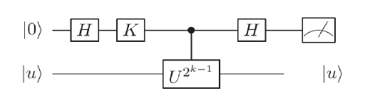
Figure 1: Hadamard test with extra phase shift operator.

For the $k_{th}$ bit position, we perform the Hadamard test depicted in Figure 1. Denote $\varphi_{k}=2^{k-1}\varphi$ and choose gate $K=I_{2}$, the probability of the post measurement state is

$$\Pr(0|k)=\frac{1+\cos(2\pi\varphi_{k})}{2},\quad\Pr(1|k)=\frac{1-\cos(2\pi\varphi_{k})}{2}.$$ (2)

By choosing the gate

$$K=\left({\begin{array}[]{cc}1&0\\ 0&i\\ \end{array}}\right)$$ (3)

as the square root of Pauli-Z ($\sigma_{z}$) gate, we have

$$\Pr(0|k)=\frac{1-\sin(2\pi\varphi_{k})}{2},\quad\Pr(1|k)=\frac{1+\sin(2\pi\varphi_{k})}{2}.$$ (4)

From the estimates of the probabilities, we have enough information to recover $\varphi_{k}$. In Kitaev’s original approach, after performing the Hadamard tests, some classical post processing is also necessary. Suppose $\varphi=0.x_{1}x_{2}\ldots x_{n}$ is an exact $n$-bit. If we are able to determine the values of $\varphi$, $2\varphi,\ldots,$ $2^{n-1}\varphi$ with some constant-precision ($1/16$ to be exact), then we can determine $\varphi$ with precision $1/2^{n}$ efficiently [7, 6].

Starting with $\varphi_{n}$ we increase the precision of the estimated fraction as we proceed toward $\varphi_{1}$. The approximated values of $\varphi_{k}\,(k=n,\ldots,1)$ will allow us to make the right choices.

For $k=1,\ldots,n$ the value of $\varphi_{k}$ is replaced by $\beta_{k}$, where $\beta_{k}$ is the closest number chosen from the set $\{\frac{0}{8},\frac{1}{8},\frac{2}{8},\frac{3}{8},\frac{4}{8},\frac{5}{8},\frac{6}{8},\frac{7}{8}\}$ such that

$$|\varphi_{k}-\beta_{k}|_{\text{mod 1}}<\frac{1}{8}.$$ (5)

The result follows by a simple iteration. Let $\beta_{n}=\overline{0.x_{n}x_{n+1}x_{n+2}}$ and proceed by the following iteration:

$$x_{k}=\left\{\begin{array}[]{l l}0&\quad\mbox{if \quad$|\overline{0.0x_{k+1}x_{k+2}}-\beta_{k}|_{\text{mod 1}}<1/4$ }\\ 1&\quad\mbox{if \quad$|\overline{0.1x_{k+1}x_{k+2}}-\beta_{k}|_{\text{mod 1}}<1/4$}\\ \end{array}\right.$$ (6)

for $k=n-1,\ldots,1$. By using simple induction, the result satisfies the following inequality:

$$|\overline{0.x_{1}x_{2}\ldots x_{n+2}}-\varphi|_{\text{mod 1}}<2^{-(n+2)}.$$ (7)

In Eq. 5, we do not have the exact value of $\varphi_{k}$. So, we have to estimate this value and use the estimate to find $\beta_{k}$. Let $\widetilde{\varphi_{k}}$ be the estimated value and

$$\epsilon=|\widetilde{\varphi_{k}}-\varphi_{k}|_{\text{mod 1}}$$ (8)

be the estimation error. Now we use the estimate to find the closest $\beta_{k}$. Since we know the exact binary representation of the estimate $\widetilde{\varphi_{k}}$, we can choose $\beta_{k}$ such that

$$|\widetilde{\varphi_{k}}-\beta_{k}|_{\text{mod 1}}\leq\frac{1}{16}.$$ (9)

By the triangle inequality we have,

$$|\varphi_{k}-\beta_{k}|_{\text{mod 1}}\leq|\widetilde{\varphi_{k}}-\varphi_{k}|_{\text{mod 1}}+|\widetilde{\varphi_{k}}-\beta_{k}|_{\text{mod 1}}\leq\epsilon+\frac{1}{16}.$$ (10)

To satisfy Eq. 5, we need to have $\epsilon<1/16$, which implies

$$|\widetilde{\varphi_{k}}-\varphi_{k}|_{\text{mod 1}}<\frac{1}{16}.$$ (11)

Therefore, it is necessary that the phase be estimated with precision $1/16$ at each stage. Let $s_{k}$ be the estimate of $\sin(2\pi\varphi_{k})$ and $t_{k}$ the estimate of $\cos(2\pi\varphi_{k})$. By Eq. 11 we should have

$$\left|\varphi_{k}-\frac{1}{2\pi}\arctan\left(\frac{s_{k}}{t_{k}}\right)\right|_{\text{mod 1}}<\frac{1}{16}.$$ (12)

To estimate the phase $\varphi_{k}$ with precision $1/16$, $s_{k}$ and $t_{k}$ must be estimated with error at most around 0.2706 [8]. By use of Chernoff bound, in order to obtain

$$\mathrm{Pr}\left(|\widetilde{\varphi_{k}}-\varphi_{k}|<\frac{1}{16}\right)>1-\varepsilon,$$ (13)

we require a minimum of

$$m\approx 76+55\ln\frac{1}{\varepsilon}$$ (14)

many trials. And by use of union bound, we desire $1-n\varepsilon\geq 3/4$. In our case $\varepsilon=\frac{1}{4n}$, hence

$$m\approx 76+55\ln 4n.$$ (15)

Therefore, for this approach the number of total unitary $U$ invocation will be

$$(76+55\ln 4n)\times(2^{n}-1).$$ (16)

2.2 Arbitrary Constant-Precision Approach

The arbitrary constant-precision approach (ACPA) draws a trade-off between the highest degree of phase shift operators being used and the depth of the circuit. As a result, when smaller degrees of phase shift operators are used, the depth of the circuit increases and vice versa. ACPA is useful when the precision of the rotation gate is limited. Let rotation gate $R_{k}$, that is precise to the $k_{th}$ degree, be defined as follows

$$R_{k}\equiv\left[{\begin{array}[]{cc}1&0\\ 0&e^{2\pi i/2^{k}}\\ \end{array}}\right].$$ (17)

A simple example of $k=3$ for estimating the third least significant eigenphase bit is given in Fig. 2.

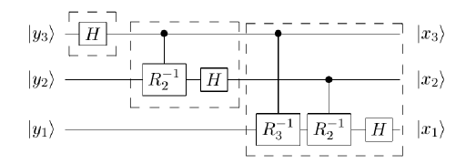
Figure 2: 3-qubit inverse QFT where $1\leq i\leq 3$, $|y_{i}\rangle=\frac{1}{\sqrt{2}}(\left|0\right>+e^{2\pi i(0.x_{i}\ldots x_{3})}\left|1\right>$.

Assume the eigenphase is $\varphi=0.x_{1}x_{2}x_{3}\ldots x_{n}$ and suppose we are at step $j$, that is we are to estimate $x_{j}$. It is clear that after applying controlled phase shift operators $R_{2}^{-1}$, $R_{3}^{-1}$, …, $R_{k}^{-1}$, we obtain

$$\left|{\widetilde{\psi_{j}}}\right\rangle=\frac{1}{\sqrt{2}}(\left|{0}\right\rangle+e^{2\pi i\widetilde{\varphi}}\left|{1}\right\rangle),$$ (18)

where

$$\widetilde{\varphi}=0.x_{j}\underbrace{00\ldots 0}_{\text{$k$ 0s}}x_{j+k}x_{j+k+1}\ldots.$$ (19)

It is easy to see that

$$|\widetilde{\varphi}-0.x_{j}|<\frac{1}{2^{k}}.$$ (20)

Hence, we can express

$$\widetilde{\varphi}=0.x_{j}+\theta.$$ (21)

The post measurement probabilities of achieving $|0\rangle$ or $|1\rangle$ where $x_{j+1}$ = 0 are

$$\Pr(0|j)=\cos^{2}(\pi\theta),\quad\Pr(1|j)=\sin^{2}(\pi\theta)$$ (22)

where $\theta<\frac{1}{2^{k}}$. Let $\tau=\frac{\pi}{2^{k-1}}$ and we can rewrite the above formula as

$$P(0|j)=\cos^{2}(\pi\theta)\geq\cos^{2}(\frac{\pi}{2^{k}})=\frac{\cos(\tau)+1}{2}.$$ (23)

By use of Taylor expansion for the cosine function, we obtain a lower bound that

$$\Pr(0|j)>1-(\tau/2)^{2}.$$ (24)

In order to achieve a success probability of $1-\varepsilon$ for estimating the $j_{th}$ bit, we can bound the required number of iterations, $m$, from below. For simplicity, let us denote $p$ as $\Pr(0|j)$ and let $X_{i}$ be the random variable for Bernoulli trials. By Chernoff bound, we have

$$\mathrm{Pr}\left(\frac{1}{m}\sum_{i=0}^{m}X_{i}\leq\frac{1}{2}\right)\geq 1-e^{-2m(p-\frac{1}{2})^{2}}=1-\varepsilon.$$ (25)

Hence, we would need at least

$$m\geq\frac{\ln(1/\varepsilon)}{2(p-1/2)^{2}}$$ (26)

trials for estimating each eigenphase bit in order to achieve success probability $1-\varepsilon$ (each bit) by use of rotation gates precise up to the $k_{th}$ degree. By Eq. 24, we know that it is sufficient to choose

$$m=\frac{2\ln(1/\varepsilon)}{{(1-\frac{(\tau)^{2}}{2})^{2}}}=\frac{2\ln(4n)}{{(1-\frac{\pi^{2}}{2^{2k-1}})^{2}}}.$$ (27)

Therefore, for this approach the number of unitary $U$ invocation will be

$$\frac{2\ln(4n)}{{(1-\frac{\pi^{2}}{2^{2k-1}})^{2}}}\times(2^{n}-1).$$ (28)

For instance, when $k=3$, this approach requires about $1/14$ of trials of Kitaev’s method to achieve the same degree of success probability for each bit. However, this rough comparison is only in terms of measurements (trials). Kitaev’s approach does not require higher degree of rotation gates, except the Hadamard. In our approach we need constant-precision rotation gates and this should be taken into account when comparing the cost.

2.3 Faster Phase Estimation

The Faster Phase Estimation (FPE) by Svore and et. al. [11] cleverly modifies Kitaev’s original approach and applies the two-stage-multiple-round strategy. By such modifications, FPE reduces the number of measurements by a logarithm factor, $\log^{*}$, in comparison to Kitaev’s approach. However, for each measurement it uses a multiple bits inference that introduces an extra logarithm factor in terms of the required number of invoking the unitary $U$.

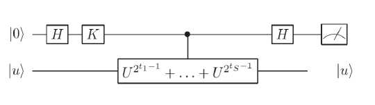
Figure 3: FPE Stage 2: Multiple Bits Inference

The algorithm contains two stages and the second stage contains multiple rounds. We list the quantum part of that algorithm in Algorithm 1 as follows:

Algorithm 1 Faster Phase Estimation

First Round:
for $j=n-1$ to $1$ do
       Estimate $2^{j-1}\varphi$ using $O(1)$ measurements per $j$.
end for
Later Rounds:
for $r$ = 2 to Number of Rounds do
       Set density, $S$, and number of measurements per bit, $s_{r}$ , for given round.
      for i = 1 to $s_{r}n$ do
            Set $M_{i}$ to a sum of $S$ different powers of two, choosing these powers of two at random
             or with a pseudo-random distribution. Perform C measurements with given $M_{i}$.
      end for
end for
Post Processing:
Perform multi-bit inference to determine estimate of $\beta_{j}=2^{j-1}\varphi$ for all $j$ from eigenphase estimates obtained in stage 1 and stage 2.
Infer eigenphase from the $\beta_{j}$s.

The first stage (see Fig. 1) is the same as Kitaev’s Hadamard tests but it requires fewer repetitions. Interested readers can refer to their work for details. The estimated eigenphase from the first stage will be used to obtain a more refined result in the second stage from multiple bits inference (see Fig. 3). We refer interested reader to [11] for details. Here we are interested in finding the constant number of repetitions, referred as C in their work, required in the second stage of FPE algorithm for resources comparison with other approaches. As shown in [11], it is necessary to obtain an estimate of $M_{i}\varphi$, let us say $\sigma_{i}$, with precision of $1/32$ and failure probability $\leq 1/8$, that is

$$\Pr[|\varphi{M_{i}}-\sigma_{i}|_{\text{mod 1}}>1/32]<1/8.$$ (29)

For simplicity, let us look at the 2-round algorithm of FPE and $M_{i}=\sum_{j\in S}2^{j}$, $S=\{s\in\mathbb{N}|1\leq s\leq n\}$ and $|S|\approx\log n$ [11]. Denote $\varphi M_{i}$ as $\varphi_{i}$. When $K=I_{2}$, the probability of the post measurement state is

$$\Pr(0|i)=\frac{1+\cos(2\pi\varphi_{i})}{2},\quad\Pr(1|i)=\frac{1-\cos(2\pi\varphi_{i})}{2}.$$ (30)

In order to recover $\varphi_{i}$, we can estimate $\Pr(0|i)$ with higher probabilities by iterating the process. But we also need to distinguish between $\varphi_{i}$ and $-\varphi_{i}$. This can be solved by the same Hadamard test in Figure 1, but instead we use the gate $K=\sqrt{\sigma_{z}}$. The probabilities of the post-measurement states based on the modified Hadamard test become

$$\Pr(0|i)=\frac{1-\sin(2\pi\varphi_{i})}{2},\quad\Pr(1|i)=\frac{1+\sin(2\pi\varphi_{i})}{2}.$$ (31)

Hence, we have enough information to recover $\varphi_{k}$ from the estimates of the probabilities.

In the first Hadamard test (Eq. 30), in order to estimate $\Pr(1|i)$ an iteration of Hadamard tests should be applied to obtain the required precision of $1/32$ (see Eq. 29) for $\varphi_{i}$. To get an estimate of $\Pr(1|i)$, we can count the number of states $\left|{1}\right\rangle$ in the post measurement state and then divide that number by the total number of iterations.

The Hadamard test outputs $\left|{0}\right\rangle$ or $\left|{1}\right\rangle$ with a fixed probability. We can model an iteration of Hadamard tests as Bernoulli trials with success probability (obtaining $\left|{1}\right\rangle$) being $p_{i}$. The best estimate for the probability of obtaining the post measurement state $\left|{1}\right\rangle$ with $\kappa$ samples is

$$\widetilde{p_{i}}=\frac{h}{\kappa},$$ (32)

where $h$ is the number of ones in $\kappa$ trials. In order to find $\sin(2\pi\varphi_{i})$ and $\cos(2\pi\varphi_{i})$, we can use estimates of probabilities in Eq. 30 and Eq. 31. Let $s_{i}$ be the estimate of $\sin(2\pi\varphi_{i})$ and $t_{i}$ the estimate of $\cos(2\pi\varphi_{i})$. It is clear that if

$$|\widetilde{p_{i}}-p_{i}|<\delta/2,$$ (33)

then

$$|s_{i}-\sin(2\pi\varphi_{i})|<\delta,\quad|t_{i}-\cos(2\pi\varphi_{i})|<\delta.$$ (34)

As the inverse tangent function is more robust to error than the inverse sine or cosine functions, we use

$$\widetilde{\varphi_{i}}=\frac{1}{2\pi}\arctan\left(\frac{s_{i}}{t_{i}}\right)$$ (35)

as the estimation of $\varphi_{i}$. By the condition given Eq. (29), the following constraint

$$\Pr[|\varphi{M_{i}}-\frac{1}{2\pi}tan^{-1}(\frac{s_{i}}{t_{i}})|\leq 1/32]_{\text{mod 1}}>7/8$$ (36)

must be satisfied.

The inverse tangent function can not distinguish between the two values $\varphi_{i}$ and $\varphi_{i}\pm 1/2$. However, because we find estimates of the sine and cosine functions as well, the correct value can be determined properly. It is easy to see, in order to estimate the phase $\varphi_{i}$ with precision $1/32$, we should make sure that

$$\left|\tan^{-1}\frac{\sin(2\pi\varphi_{i})}{\sqrt{1-\sin^{2}(2\pi\varphi_{i})}}-\tan^{-1}\frac{\sin(2\pi\varphi_{i})+\delta}{\sqrt{1-\sin^{2}(2\pi\varphi_{i})}-\delta}\right|\leq\pi/16$$ (37)

is satisfied. We obtain $\delta\leq\frac{1}{4}\sqrt{1-\frac{1}{\sqrt{2}}}$ and therefore the error of estimated probabilities should be less than $\frac{1}{8}\sqrt{1-\frac{1}{\sqrt{2}}}$. By use of the simpler bound of Chernoff-Hoeffding theorem, the number of repetition, $m$, should satisfy

$$\mathrm{Pr}\left(\left|\frac{1}{m}\sum_{i=0}^{m}X_{i}-p_{i}\right|>\frac{\delta}{2}\right)\leq 2e^{-2(\frac{\delta}{2})^{2}m}\leq 1/16.$$ (38)

Because we have to estimate both sine and cosine, the failure probability is $1/16$, instead of $1/8$. The total number of repetition is therefore $C=2m\approx 756$. The algorithm later generates the estimate of each $\beta_{j}$ that needs to satisfy

$$\Pr[|2^{j-1}\varphi-\beta_{j}|_{\text{mod 1}}>1/16]<e^{-s_{2}S}\leq 1/4n.$$ (39)

Hence, if we choose $S=\ln n$, then $s_{2}={\ln 4n}/{\ln n}$. If we are sampling from a uniform distribution for selecting $S$ different numbers for each iteration $i$, then for $s_{2}n$ iterations each unitary $U^{2^{l-1}}$ where $1\leq l\leq n$ will be summoned at least $s_{2}\cdot S\cdot C$ times. Therefore, the number of unitary $U$ invocation will be $s_{2}\cdot S\cdot C\cdot(2^{n}-1)$.

3 Cost Estimation

The cost of phase estimation comes from phase kick back and inverse quantum Fourier transform. In this section, we will compare these three approaches under the perfect and the imperfect scenarios. Suppose unitary $U$ can be decomposed into $\gamma$ logical gates. In the perfect scenario we assume that the unitary can be perfectly simulated and the cost of simulating a logical gate is one. In the imperfect case, a logical gate can only simulated imperfectly and we need to determine how the imperfection affects the required number of repetition.

3.1 Perfect Gate Generation

The cost of phase kick back is in direct proportion to the number of required measurements. As shown in the analysis in section 2, In comparison to Kitaev’s approach, even though FPE has significantly reduced the number of required measurements but it invokes at least $14$ times more than Kitaev’s in invoking the unitary $U$ for phase kick back. The cost of rotation gates only occurs in the ACPA method and the number of rotation gate invocations is

$$kn\frac{2\ln(4n)}{{(1-\frac{\pi^{2}}{2^{2k-1}})^{2}}}.$$ (40)

In comparison to the cost of the phase kick back, for any $n$ the contribution from the cost of rotation gates is negligible. The logic is that the cost in Eq. 40 will only carry a small factor for $\ln n$ with various $k$. Due to the fact that $k$ is integer and $k\geq 3$, the case where the denominator is $0$, i.e. $k\approx 2.2$, never occurs. Therefore, the cost of logical gate invocation in phase kick back in ACPA is by far larger than the cost of rotation gate invocations ($kn\ln n$ v.s. $\gamma^{2^{n}-1}$).

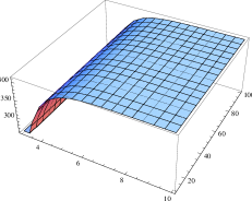
In Fig. 4 and Fig. 5, where $k\in[3,10]$ and $n\in[1,100]$, we plot the ratio between the numbers of unitary $U$ invocations among the three approaches. We can see that as $k$ goes up, we should choose ACPA as the total invocation of the unitary $U$ is significantly reduced, in comparison to those that use Hadamard test.
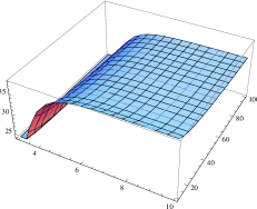
Figure 4: Ratio: Kitaev/ours. Figure 5: Ratio: FPE/ours.

Here we summarize the result in Table 1.

Case	Kitaev	Faster Phase Estimation	Ours Perfect
Measurements	$n\cdot(76+55\ln({4n}))$	$n\cdot(\log\log({4n})+C\cdot s_{2})$	$n\cdot\frac{2\ln(4n)}{{(1-\frac{\pi^{2}}{2^{2k-1}})^{2}}}$
Elementary gates	$(76+55\ln({4n}))\cdot\gamma^{2^{n}-1}$	$(\log(\log{4n})+S\cdot s_{2}\cdot C)\cdot\gamma^{2^{n}-1}$	$\frac{2\ln(4n)}{{(1-\frac{\pi^{2}}{2^{2k-1}})^{2}}}\cdot(\gamma^{2^{n}-1}+kn)$

Table 1: Phase kick back invocations. $s_{2}=\frac{\ln({4n})}{\ln n},S=\ln{n}$.

3.2 Imperfect Gate Generation

In reality, we cannot generate the rotation gate perfectly. We can only generate rotation gate $\tilde{R}_{k}$ that is $\eta$-close to rotation gate $R_{k}$. When considering the success probability of estimating each eigenphase bit, the errors propagated from imperfect gate simulations must also be considered. As mentioned in the perfect case, our approach has extra cost in the rotation gates. We need to examine the impact of imperfect rotation gates on the success probability because it directly affects the required number of repetition. Similar to the analysis in the perfect case, we have the same constraints but the analysis slightly varies. The Eq. 22 would become

$$\Pr(0|j)=\cos^{2}(\pi\tilde{\theta}),\quad\Pr(1|j)=\sin^{2}(\pi\tilde{\theta})$$ (41)

where $\tilde{\theta}=\theta+(k-1)\eta<\frac{1}{2^{k}}+(k-1)\eta$ as the error propagates from the imperfect gate simulations. Let us choose $\eta=\frac{1}{(k-1)2^{k}}$. By following the same computation logic in Eq. 23 and Eq. 24, we have the success probably of estimating the eigenphase bit correctly as

$$P(0|j)=\cos^{2}(\pi\tilde{\theta})\geq\cos^{2}(\frac{\pi}{2^{k-1}})=\frac{\cos(2\tau)+1}{2}>1-\tau^{2}$$ (42)

where $\tau=\frac{\pi}{2^{k-1}}$. Therefore, Eq. 27 can be rewritten as

$$m=\frac{2\ln(1/\varepsilon)}{{(1-2(\tau)^{2}})^{2}}=\frac{2\ln(4n)}{{(1-\frac{\pi^{2}}{2^{2k-3}})^{2}}}$$ (43)

in this scenario. It is clear to see that the result is almost identical to the perfect case, except the value of $k$ in the perfect case is now shifted to the left by 1 in the imperfect case. From Fig. 6 we know that the smallest ratio occurs when $3<k<4$ (to be exact, it should be around $3.2$ as the imperfect case is the perfect case shifted to the left by 1). When $k=3$, the ratio is about $1.7$ and when $k=4$, the ratio is around $14$ . Because $k$ must be an integer in our case, we know that in the imperfect case the number of required repetition is still smaller than other the two approaches. Hence, the number of unitary $U$ invocations in our approach still requires fewer resources.

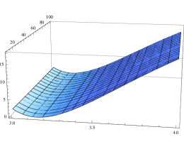
Figure 6: Ratio: Kitaev/ours.

There are some clever approaches [5, 12] for simulating rotation gates. For instance, in a recent paper [12], the authors show the cost of such a gate is $O(\log^{c}(1/\eta))$ where $1.12\leq c\leq 2.27$ and $\eta$ is the rotation angle error. In Solovay-Kitaev’s decomposition theorem, $c$ is around $3.94$ and is bounded from below by $1$. By applying the cost function given in the decomposition theorem, the extra cost in ACPA would be

$$kn\cdot\frac{2\ln(4n)}{{(1-\frac{\pi^{2}}{2^{2k-3}})^{2}}}\cdot O(\log^{c}(1/\eta))=O((k+\log k)^{c}(kn\cdot\frac{2\ln(4n)}{{(1-\frac{\pi^{2}}{2^{2k-3}})^{2}}})).$$ (44)

Similar to the argument in the perfect case, the extra cost ($O((k+\log k)^{c}(kn\ln n))$ v.s. $\gamma^{2^{n}-1}$) is negligible (by use of L’Hôpital’s rule) when $n$ is large and $k$ is small (as we are discussing constant precision rotation gates) and $c$ is a constant less than 4.

4 Discussion

In this work, we are analyzing the three approaches solely in terms of the circuit complexity. Hence, it pays off if higher degree of rotation gates can be implemented as it significantly reduces the cost from phase kick back. However, if we need to consider time complexity when multiple eigenvectors are available and higher degrees of rotation gates are unfeasible, Hadamard test based approaches should be chosen as they can be run in parallel while the ACPA can be run partially in parallel.

5 Acknowledgments

C. C gratefully acknowledges the support of Lockheed Martin Corporation. We also like to thank J. Anderson, P. Iyer and D. Poulin for useful comments and suggestions.

References

- [1] P. W. Shor, Polynomial-time algorithms for prime factorization and discrete logarithms on a quantum computer, SIAM J. Comp., 26, no. 5, pp. 1484–1509, 1997
- [2] M. Szegedy, Quantum speed-up of markov chain based algorithms, 45th Ann. IEEE Symp. Found., pp. 32–41, 2004
- [3] P. W. Shor, Algorithms for quantum computation: discrete logarithms and factoring, 35th Ann. IEEE Symp. Found. (Santa Fe, NM, pp. 124–134, 1994
- [4] G. Brassard, P, Høyer, A. Tapp, Lecture Notes in Computer Science, vol. 1443, pp 820–831, Springer, 1998
- [5] M. A. Nielsen and I. L. Chuang, Quantum computation and quantum information, Cambridge: Cambridge University Press, 2000
- [6] A. Kitaev, A. H. Shen and M. N. Vyalyi, Classical and quantum computation, Providence, RI: American Mathematical Society, 2002
- [7] A. Kitaev, Quantum measurements and the Abelian stabilizer problem, technical report., 1996
- [8] H. Ahmedi and C. Chiang, Quantum phase estimation with arbitrary constant-precision phase shift operators, Quantum Information and Computation, vol. 12, no. 9&10, pp. 0864–0875, 2012
- [9] D. Cheung, Improved Bounds for the approximate QFT, Proceedings of the Winter International Symposium on Information and Communication Technologies (WISICT), pp. 1–6, Trinity College Dublin, 2004
- [10] P. Kaye, R. Laflamme and M. Mosca, An introduction to quantum computing, Oxford: Oxford University Press, 2007
- [11] K. Svore, M. Hastings and M. Freedman, Faster Phase Estimation, arXiv:1304.0741
- [12] G. Duclos-Cianci and K. Svore, A state distillation protocol to implement arbitrary single-qubit rotations, arXiv:1210.1980v1