Quantum Phase Estimation with an Arbitrary Number of Qubits

Abstract

Due to the great difficulty in scalability, quantum computers are limited in the number of qubits during the early stages of the quantum computing regime. In addition to the required qubits for storing the corresponding eigenvector, suppose we have additional $k$ qubits available. Given such a constraint $k$, we propose an approach for the phase estimation for an eigenphase of exactly $n$-bit precision. This approach adopts the standard recursive circuit for quantum Fourier transform (QFT) in [1] and adopts classical bits to implement such a task. Our algorithm has the complexity of $O(n\log k)$, instead of $O(n^{2})$ in the conventional QFT, in terms of the total invocation of rotation gates. We also design a scheme to implement the factorization algorithm by using $k$ available qubits via either the continued fractions approach or the simultaneous diophantine approximation.

1 Introduction

Quantum phase estimation (QPE) is a key quantum operation in many quantum algorithms [2, 3, 4, 5, 6]. Phase estimation is extensively used to solve a variety of problems, such as hidden subgroup, graph isomorphism, quantum walk, quantum sampling, adiabatic computing, order-finding and large number factorization. QPE comprises two components: phase kick back and inverse quantum Fourier transform. The implementation of quantum Fourier transform has been described in numerous research articles [1, 7, 8, 9, 10]. The physical implementation (algorithms based on quantum Fourier transform (QFT)) is highly constrained by the requirement of (1) high-precision controlled rotation gates (phase shift operators), which remain difficult to realize, and (2) sufficient number of qubits to approximate the eigenphase to a required precision.

At the early stage of a quantum computing implementation, we can imagine that scalability could be an issue. The quantum resources could be limited, in terms of available quantum qubits and quantum gates. From that perspective, efficient implementations of quantum algorithms are essential when available quantum resources are scarce. For instance, Parker and Plenio [12] show that a single pure qubit together with a collection of $\log_{2}N$ qubits in an arbitrary mixed (or pure) state is sufficient to implement Shor’s factorization algorithm efficiently to factorize a large number $N$. Such implementation addresses the issue of limited qubits but introduces the concern for the decoherence.

In this paper, we are interested in the following two aspects. (1) Given certain available qubits, assuming $k+\log_{2}N$ qubits in total, we want to have an efficient way to implement quantum phase estimation and use as few controlled rotation gates (c-r.g.) as possible. (2) Apply this technique to Shor’s factorization algorithm along with simultaneous diophantine approximation [13] to investigate the feasible implementation structure when the available qubits are limited. We assume only one copy of the eigenvector $|u\rangle$ (requiring $\log_{2}N$ qubits) and additional $k$ qubits are available. One copy of the eigenvector implies a restriction on the use of controlled-U gates: all controlled-U gates should be applied on the workspace register ($k$ qubits).

One copy of an eigenvector is a reasonable assumption because multiple copies of $|u\rangle$ would imply the requirement for extra multiple of $\log_{2}N$ qubits for storage. Hence, it is practical as we are considering the case that the available qubits are scarce. Thus, the entire process is a single circuit ($\lceil n/k\rceil$ stages) that can not be divided into parallel processes. Under such an assumption, for approaches that require repetitions, such as Kitaev’s [7] and others [9], parallelization can not be done and the circuit depth is the same as the size of the circuit. On the other hand, if we have enough qubits for storing multiple copies of eigenvector $|u\rangle$, we should choose Kitaev’s approach because the processes can thus be run in parallel. Throughout the rest of the article, we will refer to the $k$ available qubits as the qubits used in the workspace register.

Generally speaking, quantum circuits for QFT implemented in different approaches [1, 7, 8, 9, 10] would require the same number of controlled-U gates but different numbers of rotation gates. We are interested in using the recursive approach, along with some classical resources, to implement the inverse quantum Fourier transform. We bound the number of required rotation gates from above.

We give an overview of the conventional quantum phase estimation technique in section 2. We detail our algorithms and the analysis in section 3, including a brief analysis of Kitaev’s original approach [7]. An application of our approach along with simultaneous diophantine approximation to the factorization problem is given in section 3.4. Finally we state our conclusion in section 4.

2 Approach based on QFT

One of the standard methods to approximate the phase of a unitary matrix is QPE based on QFT. The structure of this method is depicted in Figure 1.

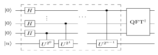
Figure 1: Standard QPE with $n$ qubits as ancilla. The dash-line box is the phase kickback.

The QPE algorithm requires two registers and contains two stages. Suppose the eigenphase of unitary $U$ is $\varphi=0.\varphi_{1}\varphi_{2}\ldots\varphi_{n}$ in the binary representation such that

$$U|u\rangle=e^{2\pi i\varphi}|u\rangle.$$ (1)

Then the first register is prepared as a composition of $n$ qubits initialized in the state $|0\rangle$. The second register is initially prepared in the state $|u\rangle$. The first stage prepares a uniform superposition over all possible states and then applies controlled-$U^{2^{l}}$ operations. Consequently, the state becomes

$$\frac{1}{2^{n/2}}\sum_{l=0}^{2^{n}-1}e^{2\pi i\varphi l}|l\rangle.$$ (2)

The second stage in the QPE algorithm is the QFT^† operation. At each step (starting from the least significant bit) by using the information from previous steps, the inverse Fourier transform transforms the state

$$\frac{1}{\sqrt{2}}(|0\rangle+e^{2\pi i2^{l}\varphi}|1\rangle)$$ (3)

to get closer to one of the states

$$\frac{1}{\sqrt{2}}(|0\rangle+e^{2\pi i0.0}|1\rangle)=\frac{1}{\sqrt{2}}(|0\rangle+|1\rangle)\quad\mbox{or}\quad\frac{1}{\sqrt{2}}(|0\rangle+e^{2\pi i0.1}|1\rangle)=\frac{1}{\sqrt{2}}(|0\rangle-|1\rangle).$$ (4)

Suppose $\varphi$ is precise to the $3$rd bit, that is $\varphi=0.\varphi_{1}\varphi_{2}\varphi_{3}$. As shown in Figure 2, each step (dashed-line box) uses the result of previous steps, where phase shift operators are defined as

$$R_{l}\equiv\left[{\begin{array}[]{cc}1&0\\ 0&e^{2\pi i/2^{l}}\\ \end{array}}\right]$$ (5)

for $2\leq l\leq 3$. By concatenating $\varphi_{1}$, $\varphi_{2}$ and $\varphi_{3}$, we obtain $\varphi$. Therefore, when $\varphi$ is precise to the $n_{th}$ bit, the total number of rotation gate invocations is $O(n^{2})$.

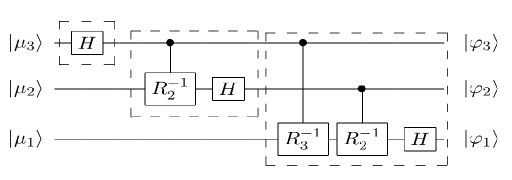
Figure 2: 3-qubit inverse QFT where $1\leq j\leq 3$, $|\mu_{j}\rangle=\frac{1}{\sqrt{2}}(\left|0\right>+e^{2\pi i(0.\varphi_{j}\ldots\varphi_{3})}\left|1\right>$).

3 Our Algorithm

Before proceeding to our algorithm, we provided the description of the recursive circuit for quantum Fourier transform [1] technique. In [1], in addition to the recursive circuit, the authors also adopted the technique by Schönhage and Strassen [14] for integer multiplication. However, the integer multiplication is performed via classical computation. We use the classical bits and operators to compute the parameter (the desired phase shift) of a quantum rotation gate. The algorithm structure is explained in subsection 3.2.

3.1 Standard recursive circuit description for $F_{2^{n}}^{\dagger}$

Let $F_{2^{n}}^{\dagger}$ denote the inverse Fourier transform modulo $2^{n}$ that acts on $n$ qubits. The standard quantum circuit for $F_{2n}^{\dagger}$ can be described recursively as follows. Let us denote this circuit as $RF_{2^{n}}^{\dagger}$.

1. Suppose the state of the work register after phase kickback is

   $$|\psi\rangle=\frac{1}{\sqrt{2}}(|0\rangle+e^{2\pi i0.\varphi_{1}\ldots\varphi_{n}}|1\rangle)\otimes\ldots\otimes\frac{1}{\sqrt{2}}(|0\rangle+e^{2\pi i0.\varphi_{n}}|1\rangle)=|\mu_{1}\rangle\otimes\ldots\otimes|\mu_{n}\rangle$$ (6)

2. Apply $F_{2^{m}}^{\dagger}$ to the last m qubits ($|\mu_{n-m+1}\rangle\otimes\ldots\otimes|\mu_{n}\rangle$).

3. Read out and store the values of the $m$ qubits in classical bits ($c_{1}\ldots c_{m}$).

4. Compute rotation angle: $f(c_{1}\ldots c_{m})=\sum_{i=1}^{m}(\frac{1}{2})^{i}\cdot c_{i}$.

5. For each $j\in\{1,2,\ldots,n-m\}$, apply the rotation gate $R_{\frac{f(c_{1}\ldots c_{m})}{2^{n-m-j+1}}}^{\dagger}$ to the $j^{th}$ qubit. Here the rotation gate $R_{\frac{f(c_{1}\ldots c_{m})}{2^{n-m-j+1}}}^{\dagger}$ is defined as

   $$R_{q}^{\dagger}=\left(\begin{array}[]{cc}1&0\\ 0&e^{-2\pi i\frac{f(c_{1}\ldots c_{m})}{2^{n-m-j+1}}}\end{array}\right)$$

6. Apply $F_{2^{n-m}}^{\dagger}$ to the first $n-m$ qubits.

For simplicity, let us assume that $n$ is some power of 2. Then step 5 is the step that resets the disturbing eigenphase bits for the first $n-m$ qubits because all the disturbing eigenphase bits from the last $m$ bits will be cleared. The number of required rotation operations for such a step is $n/2$ (suppose we choose $m=n/2$) as we have to reset for each qubit in the last $n-m$ qubits.

It is clear to that the total number of required rotation gates is

$$T_{n}=T_{n/2}+T_{n/2}+n/2$$ (7)

where $T_{1}=1$. Hence, the complexity is $O(n\log n)$ for such a recursive circuit.

3.2 The algorithm structure

Given $k$ ancillary bits initialized in $|0\rangle$ and eigenvector $|u\rangle$ of unitary $U$ where $U|u\rangle=e^{2\pi i\varphi}|u\rangle$ as input, we want to estimate the eigenphase of $U$ precise to the $n_{th}$ bit. The algorithm comprises $\lceil n/k\rceil$ stages that run in sequence. At each stage, we perform phase kickback, controlled-rotation operation and recursive inverse Fourier transform to obtain $k$ eigenphase bits. Once the last stage finishes, we can concatenate the obtained eigenphase bits, resulting in an estimated eigenphase of $\varphi$. For the details, please refer to Algorithm 1 listed below.

Algorithm 1 Phase Estimation with Variable Number of qubits

Input: $k$ ancillary bits initialized in $|0\rangle$ and eigenvector $|u\rangle$ of unitary $U$ where $U|u\rangle=e^{2\pi i\varphi}|u\rangle$.

Step I:
At stage $j$, where $j\in\{1,\ldots,\lceil n/k\rceil\}$, run phase kick back on $k$ qubits by using the controlled $U^{2^{l}}$ operations. Note that $l\in\{{n-jk},{n-jk+1},\ldots,{n-(j-1)k-1}\}$.

Step II:
For $t\in\{1,\ldots,k\}$, apply the rotation gate $R_{\frac{F[j-1]}{2^{k-t+1}}}^{\dagger}$ to the $t_{th}$ qubit.
Apply the generalized recursive circuit $F_{2^{k}}^{\dagger}$.
Read out the result to $k$ classical bits $(c_{1}\ldots c_{k})$ (the actual label is $c_{n-jk+1}\ldots c_{n-(j-1)k}$).
Compute the value $F[j]=f(c_{1}\ldots c_{k})+\frac{F[j-1]}{2^{k}}$ where $f(c_{1}\ldots c_{k})=\sum_{i=1}^{k}(\frac{1}{2})^{i}\cdot c_{i}$.
Reset $k$ qubits to $|0\rangle$

Step III:
Repeat Step I and Step II $\lceil n/k\rceil$ times (i.e. $\lceil n/k\rceil$ stages)

Output:
Concatenate the $n$ classical bits $c_{1},\ldots,c_{n}$, resulting in an estimated eigenphase $\varphi=0.c_{1}c_{2}c_{3}\ldots$.

Let us write the eigenphase $\varphi$ in the binary presentation as $0.\varphi_{1}\ldots\varphi_{n}$. Let $|\psi\rangle=|0\rangle^{\otimes k}|u\rangle$ be the initial state at stage $j$ before the phase kickback. After Step I, we obtain the state

$$|\Phi\rangle_{1}=\frac{1}{\sqrt{2}}(|0\rangle+e^{2\pi i0.\varphi_{n-jk+1}\ldots\varphi_{n-1}\varphi_{n}}|1\rangle)\otimes\ldots\otimes\frac{1}{\sqrt{2}}(|0\rangle+e^{2\pi i0.\varphi_{n-jk+k}\ldots\varphi_{n-1}\varphi_{n}}|1\rangle).$$ (8)

It is clear to see that for the $t_{th}$ qubit that the eigenphase discovered from previous stages is shifted to the right by $k-t+1$ bits in the binary presentation. At the beginning of Step II, by applying the rotation gate $R_{\frac{1}{2^{k-t+1}}\cdot F[j-1]}^{\dagger}$ , we reset the discovered eigenphase in those $k$ qubits. Hence, we obtain the state

$$|\Phi\rangle_{2-1}=\frac{1}{\sqrt{2}}(|0\rangle+e^{2\pi i0.\varphi_{n-jk+1}\ldots\varphi_{n-jk+k}}|1\rangle)\otimes\ldots\otimes\frac{1}{\sqrt{2}}(|0\rangle+e^{2\pi i0.\varphi_{n-jk+k}}|1\rangle).$$ (9)

Now we have reduced the scenario to the case where the disturbing eigenphase bits from previous stages are reset to $0$. Hence we can use the general recursive circuit for the inverse quantum Fourier transform to obtain the eigenphase bits ($\varphi_{n-jk+1},\varphi_{n-jk+2},\ldots,\varphi_{n-jk+k}$).

Once we obtain the $k$ eigenphase bits, we can read out and store them in classical bits to compute $F[j]$. We refer interested readers to [17] for the details in this semiclassical approach. The value, $F[j]$ will be used again in the next stage for resetting the previous $j\times k$ eigenphase bits. Figure 3 depicts the process of a single iteration.

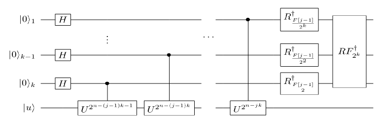
Figure 3: At stage $j$: with $k$ qubits as ancilla, $k$ rotation operations and one $RF_{2^{k}}^{\dagger}$ operation.

3.3 The Analysis

The cost of our algorithm has two parts: classical and quantum. For the classical part, we need $n$ classical bits, $k+2$ doubles and $k+2$ classical operators. $n$ classical bits are used to store all of the observed eigenphase bits. At any given stage (say $j$), two primitive doubles, $X$ and $Y$ are required such that we have

$$X=F[j],\quad Y=F[j-1].$$

To generate $k$ different rotation angle operators (see the first substep of Step II in Algorithm 1), we need $k$ doubles ($Reg[k]$, an array of $k$ doubles) and $k$ operators to generate the parameter,

$${\frac{F[j-1]}{2^{k-t+1}}},$$

of a quantum rotation gate for the $t_{th}$ qubit at the $j_{th}$ iteration where $t\in\{1,2,\ldots,k\}$.

Once the $k$ eigenphase bits are stored in classical bits in the $j_{th}$ iteration, a classical operator computes $F[j]$ such that

$$F[j]=X=f(c_{1}\ldots c_{k})+\frac{Y}{2^{k}}.$$

Then another operator sets $Y=X$. By doing so, double $X$ and $Y$ can be reused in the next iteration. Therefore, classically $n$ classical bits, $k+2$ doubles and $k+2$ classical operators are needed. The same device (classical requirement) can be used inside the recursive circuit since our approach is sequential, not parallelled. The classical requirements are summed in Table 1.

Table 1: Required classical bits

Register Type	Required number of bits
$X$ (classical register)	64
$Y$ (classical register)	64
Reg$[k]$ (classical register)	64$k$
Classical bits for eigenphase	$n$

For the quantum part, the number of total rotation gate invocations in our approach would be

$$k\log k+(\lceil n/k\rceil-1)((k+k\log k))\approx O(n\log k).$$ (10)

The reasoning is as follows. At stage $j=1$, the rotation operations only occur inside the recursive inverse Fourier transform $RF_{2^{k}}$ as $F[0]=0$. For stage $j=2,\ldots,\lceil\frac{n}{k}\rceil$, it is required to have rotation gates $R^{\dagger}_{\frac{F[j-1]}{2^{k-t+1}}}$, where $1\leq t\leq k$, to reset the dangling eigenphase bits before the recursive inverse Fourier transform $RF_{2^{k}}$. Based on the cost fuction for $RF_{2^{k}}$ derived in Eqn. 7, we obtain the cost for our approach as shown in Eqn. 10.

For comparison with other known existing approaches, in the following section we will briefly describe the analysis and the result rendered in [9] regarding Kitaev’s original approach [7].

3.3.1 Kitaev’s Original Approach

In this approach, a series of Hadamard tests are performed for each eigenphase bit in order to recover the phase correctly. Suppose the precision up to the $n$th bit is required, then in each test the phase $\phi_{l}=2^{l-1}\varphi$ ($1\leq l\leq n$) must be computed up to precision $1/16$. We perform the Hadamard test on the $l_{th}$ eigenphase bit, starting from $l=n$ down to $1$, as depicted in Figure 4.

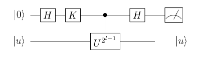
Figure 4: Hadamard test with extra phase shift operator.

When $K=I_{2}$, the probabilities of post-measurement of the Hadamard test are

$$\Pr(0|k)=\frac{1+\cos(2\pi\varphi_{k})}{2},\quad\Pr(1|k)=\frac{1-\cos(2\pi\varphi_{k})}{2}.$$ (11)

However, a cosine cannot distinguish $\phi_{l}$ and $-\phi_{l}$. We need to choose $K=\left({\begin{array}[]{cc}1&0\\ 0&i\\ \end{array}}\right)$ to be able to distinguish. The probabilities of the post-measurement states based on the modified Hadamard test become

$$\Pr(0|l)=\frac{1-\sin(2\pi\phi_{l})}{2},\quad\Pr(1|l)=\frac{1+\sin(2\pi\phi_{l})}{2}.$$ (12)

We then can recover $\phi_{l}$ from the estimates of the probabilities. To obtain the required precision of $1/16$ for $\phi_{l}$, we can run an iteration of Hadamard tests to estimate $\Pr(1|l)$ to some precision.

Theorem 1.

[9] Assume $U$ is a unitary matrix with eigenvalue $e^{2\pi i\varphi}$ and corresponding eigenvector $|u\rangle$. Suppose $\varphi=0.\varphi_{1}\ldots\varphi_{n}$ and let $\phi_{l}=2^{l-1}\varphi$ ($1\leq l\leq n$). To obtain the required precision of $1/16$ for $\phi_{l}$ such that the recovered $\tilde{\varphi}$ is precise to the $n$th bit with constant success probabilty greater than $\frac{1}{2}$, for each $\phi_{l}$ we need to run at least $55\ln n$ trials of Hadamard tests when using Kitaev’s approach.

We refer the interested readers to [9] for the details. Since we have $n$ stages for $\phi_{l}$, the required invocation of a rotation gate (Hadamard in this case) in Kitaev’s approach is $O(n\ln n)$. Suppose the controlled-rotation gates are precise, we list the comparison between Kitaev’s approach, the conventional QFT based approach and our approach in Table 2.

Table 2: The number of quantum rotation gates invocations

Approach Type	Conventional	Kitaev’s	Ours
Complexity	$O(n^{2})$	$O(n\ln n)$	$O(n\log k)$

3.4 An Application

In this section, we will focus on how to use $k$ available qubits to implement the quantum factorization algorithm. Shor’s factorization algorithm provides a polynomial approach to factorize a large number $N$. Suppose $N$ is an $L$ bit composite number of interest. There is no known classical algorithm for factoring in only polynomial time, i.e., that can factor in time $O(L^{c})$ for some constant $c$. The most difficult integers to factor in practice using existing algorithms are those that are products of two large primes of similar size, and for this reason these are the integers used in cryptographic applications. The largest such semiprime yet factored was RSA-768, a 768-bit number with 232 decimal digits [15].

Quantumly, it is shown such a task can be done by using $O(L^{3})$ operations. The algorithm is two-fold. It first runs phase estimation to obtain the eigenphase $\varphi=0.\varphi_{1}\varphi_{2}\ldots\approx s/r$ where $r$ is the order of an arbitrary element $x$ (that is $x^{r}=1($mod $N)$). The second part of the algorithm involves the continued fractions algorithm to approximate $s/r$, based on the eigenphase we obtain in phase estimation, in order to recover the order $r$. If $r$ is even, then we know that $(x^{r/2}+1)(x^{r/2}-1)=0($mod $N)$ and we successfully factorize $N$ into a product of two large numbers of similar size.

However, using the continued fraction algorithm leads inevitably to a squaring of the number to be factored. This follows from the following theorem.

Theorem 2.

[8] Suppose $s/r$ is a rational number such that

$$\big{|}\frac{s}{r}-\varphi\big{|}\leq\frac{1}{2r^{2}}.$$

Then $s/r$ is a convergent of the continued fraction for $\varphi$, and thus can be computed in $O(L^{3})$ operations using the continued fractions algorithm.

This in turn doubles the length, approximately to $2L+1$ qubits, of the quantum registers in order to achieve required precision $1/2r^{2}$ since $1\leq r\leq N\leq 2^{L}$. Park and Plenio [12] show that they can implement the algorithm by use of $1$ qubit along with the semiclassical approach [17]. For such a design, the whole circuit (quantum-wise) consists of $2L+1$ stages of recovering $\varphi_{i}$, where $1\leq i\leq 2L+1$, and calculating a controlled rotation for the next stage. After obtaining all the $\varphi_{i}$, the post processing (continued fractions) recovers the order $r$.

In the work by Seifert[13], he proposes an alternative to approximate the order by using the simultaneous diophantine approximation [16]. The theorem is as follows.

Theorem 3.

[13] Let $N$ be the product of two randomly chosen primes of equal size, i.e. of the same length in the binary representations. There exists a randomized polynomial-time quantum algorithm that factors $N$ and uses quantum registers of binary length $\lceil(1+\epsilon)\log N\rceil$, where $\epsilon$ is an arbitrarily small positive constant .

In such a design, more computations are shifted from the quantum computation part to the classical computation part, in comparison to Shor’s algorithm. This might be of importance to practical realizations of a quantum computer. It is also clear that the simultaneous diophantine approach only requires $(1+\epsilon)\log N$ qubits, that is the precision requirement of $\frac{1}{2^{L(1+\epsilon)}}$ for the phase estimation, to guarantee the existence of a polynomial quantum algorithm for the factorization problem.

Given the constraint that we only have $k$ qubits available for implementation, we have the following scheme.

Algorithm 2 Factorization: Choice of Approximation Approach

Input: $k$ ancillary bits initialized in $|0\rangle$ and eigenvector $|u\rangle$ of unitary $U$ where $U|u\rangle=e^{2\pi i\varphi}|u\rangle$.

Case I: Continued Fractions
Choose $n=2L+1$.
Run algorithm 1 to approximate $\varphi$ and the number of stages is $\lceil\frac{2L+1}{k}\rceil$.
Run the continued fractions algorithm to recover the order $r$ from the approximated $\varphi$.

Case II: Diophantine Approximation
Choose $n=L(1+\epsilon)$.
Run algorithm 1 to approximate $\varphi$ and the number of stages is $\lceil\frac{L(1+\epsilon)}{k}\rceil$.
Run the simultaneous diophantine approximation algorithm to recover the order $r$ from the approximated $\varphi$.

Clearly this is the tradeoff between the computational complexity (even though both are polynomial) and the available qubits. Quantumly they both have the same number of invocation of the unitary $U$. However, based on Eq. 10, the number of total quantum rotation gates invocation in the first case is approximately $(2L+1)\log k+(2L+1)-k$ while that of the second case is approximately $L(1+\epsilon)\log k+L(1+\epsilon)-k$. At the early stage of a quantum computing implementation, $k$ is probably significantly less than $L$. In such a scenario, the number of total rotation gate invocation in the first case is approximately twice of that in the second case.

Furthermore, another important issue we need to consider is the decoherence. Despite the fact that the complexity for case I is smaller (classically), it is more costly quantumly. The difference in quantum resources might be amplified when the implementation of error correction is considered as the first case has more stages and more rotation gate invocations.

4 Conclusion

We expect the cost of classical computation to be fairly inexpensive in comparison to its quantum counterpart. Our approach provides a way to obtain the eigenphase when the number of available qubits is rather limited. It invokes $O(n\log k)$ rotation gates and this gain comes from (1) the use of recursive circuits for $QFT^{\dagger}$ and (2) the use of the classical bits and classical operators.

Another obstacle of high-precision rotation gates (phase shift operators) is not addressed yet. For future work, we could combine with another approach [9] to approximate the eigenphase with variable number of qubits and arbitrary constant-precision operators.

5 Acknowledgments

C. C gratefully acknowledges the support of Lockheed Martin Corporation and NSF grants CCF-0726771 and CCF-0746600. We would like to thank David Poulin and Pawel Wocjan for useful comments and suggestions.

References

- [1] R. Cleve and J. Watrous, Fast Parallel Circuits for Quantum Fourier Transform, Proceedings of 41st Annual Symposium on Foundations of Computer Sciences, pp. 526–536, 2000.
- [2] S. Hallgren, Polynomial-time Quantum Algorithms for Pell’s Equation and the Principal Ideal Problem. In Proceedings of the 34th ACM Symposium on Theory of Computing, 2002.
- [3] P. Shor, Algorithms for Quantum Computation: Discrete Logarithms and Factoring. Proceedings of FOCS, pg. 124-134, 1994.
- [4] P. Shor, Polynomial-time Algorithms for Prime Factorization and Discrete Logarithms on a Quantum Computer. SIAM Journal on Computing, 26(5):1484-1509, 1997.
- [5] M. Szegedy, Quantum Speed-up of Markov Chain Based Algorithms, Proc. of 45th Annual IEEE Symposium on Foundations of Computer Science, pp. 32–41, 2004.
- [6] P. Wocjan, C. Chiang, D. Nagaj and A. Abeyesinghe, A Quantum Algorithm for Approximating Partition Functions, Physical Review A, vol. 80, pp. 022340, 2009.
- [7] A. Kitaev, A. Shen and M. Vyalyi, Classical and Quantum Computation, vol. 47, Graduate Studies in Mathematics, American Mathematical Society, 2002.
- [8] M. Nielsen and I. Chuang, Quantum Computation and Quantum Information, Cambridge University Press, 2000.
- [9] H. Ahmedi and C. Chiang, Quantum Phase Estimation with Arbitrary Constant-precision Phase Shift Operators, Quantum Information and Computation, vol. 12, no. 9&10, pp. 0864–0875, 2012.
- [10] D. Cheung, Improved Bounds for the Approximate QFT, Proceedings of the Winter International Symposium on Information and Communication Technologies (WISICT), pp. 1–6, Trinity College Dublin, 2004.
- [11] A. Kitaev, Quantum measurements and the Abelian stabilizer problem, technical report, 1996.
- [12] S. Parker and M. Plenio, Efficient Factorization with a Single Pure Qubit and logN Mixed Qubits, Phys. Rev. Lett. vol. 85, issue 14, pp. 3049–3052, 2000.
- [13] J. Seifert, Using Fewer Qubits in Shor’s Factorization Algorithm Via Simultaneous Diophantine Approximation, Proceedings of the Conference on Topics in Cryptology, pp. 319–327, 2001.
- [14] A. Schönhage and V. Straßen, Schnelle Multiplikation Großer Zahlen, Computing, vol. 7, no. 3, pp. 281–292, 1971.
- [15] T. Kleinjung, et al, Factorization of a 768-bit RSA modulus, International Association for Cryptologic Research. Retrieved 2010-08-09.
- [16] J. Lagarias, The Computational Complexity of Simultaneous Diophantine Approximation Problems, SIAM Journal on Computing, vol. 14, issue 1, pp. 196-209, 1985.
- [17] R. Griffiths and C. Niu, Semiclassical Fourier Transform for Quantum Computation, Phys. Rev. Lett. 76, 3228, 1996.