A Mathematical Aspect of A Tunnel-Junction
for Spintronic Qubit

Abstract

We consider the Dirac particle living in the $1$-dimensional configuration space with a junction for a spintronic qubit. We give concrete formulae explicitly showing the one-to-one correspondence between every self-adjoint extension of the minimal Dirac operator and the boundary condition of the wave functions of the Dirac particle. We then show that the boundary conditions are classified into two types: one of them is characterized by two parameters and the other is by three parameters. Then, we show that Benvegnù and Da̧browski’s four-parameter family can actually be characterized by three parameters, concerned with the reflection, penetration, and phase factor.

1 Introduction

The current cutting-edge technology has developed seeking the realization of quantum information and quantum computation. For such realization, the mathematical modeling of the system of some quantum devices will play an important role. One of the candidates for qubit is electron spin, that is, the so-called electron-spin qubit or the spintronic qubit, from the point of the view of spintronics [5, 9, 12, 21, 22, 23]. It is remarkable that the transportation of a single electron as a qubit has been demonstrated experimentally [17, 24] as well as the spin-conserved transport tunneling through a junction was experimentally demonstrated in organic spintronics [28, 36]. In addition, the spin-flip and the phase-shift was demonstrated in the experiment for the spin state of an electron-hole pair in a semiconductor quantum dot [16], while the spin alignment was studied in the process of the spin-transport in organic spintronics [29]. The experimental development makes us hopeful that an integrated circuit for qubit and a quantum network are really demonstrated in future.

This paper deals with the Dirac particle living in the configuration space consisting of the two quantum wires and a junction for the spintronic qubit. Although we actually have to determine a concrete physical object for the junction, we regard the junction as a black box so that it has mathematical arbitrariness. We regard the wires as the union of the intervals, $(-\infty,-\Lambda)\cup(\Lambda,\infty)$, $\Lambda\geq 0$, for mathematical simplicity. Namely, the segment $[-\Lambda,\Lambda]$ with length $2\Lambda$ plays a role of the junction. Many physicists have investigated the individual boundary condition of the wave functions of the Dirac particle for the corresponding self-adjoint extension of the Dirac operator in the case of the point interaction (i.e., $\Lambda=0$) [1, 2, 8, 14, 30]. Meanwhile, the Dirac operator consists of the combination of the Dirac matrices and the momentum operator of electron. The boundary conditions of the self-adjoint extensions of the momentum operators have been studied by mathematicians [18, 26]. We note that there is a general theory in mathematics, called boundary triple, to handle the boundary condition, and the theory has still been developed [6, 7, 11, 10, 13]. In Refs.[15, 31] the appearance of a phase factor was proved for the Schrödinger particle under the same mathematical set-up as ours. For our Dirac particle, in the case where $\Lambda=0$, Benvegnù and Da̧browski showed that a phase factor appears in their four-parameter family (see Eq.(15) of Ref.[8]). In addition, they showed how the boundary condition affects the spin. The description of boundary condition by the individual one-parameter families have been studied in Refs.[1, 14, 20, 30] (also see Eqs.(17) and (18) of Ref.[8]). We will go ahead and make an in-depth research for the Dirac particle. Thus, we employ the minimal Dirac operator for the Hamiltonian. In this paper, we follow the machinery in Refs.[8, 15, 18, 26, 31] based on the von Neumann’s theory [27, 34], in which all the self-adjoint extensions of our minimal Dirac operator are parameterized by $U\in U(2)$, where $U(2)$ is unitary group of degree $2$.

We prove that all the boundary conditions of wave functions of our Dirac particle are completely classified into the two types (See Corollary 4.5). One of them is the type that states the wave functions do not pass through the junction, and described by two parameters, $\gamma_{L},\gamma_{R}\in\mathbb{C}$ with $|\gamma_{L}|=|\gamma_{R}|=1$, concerned with the reflections at $-\Lambda$ and at $+\Lambda$, respectively. The other is the type that states the wave functions do pass through the junction, and described by Benvegnù and Da̧browski’s four-parameter family (see Theorem 4.2, Theorem 4.4, and Proposition 4.7). We give our concrete formulae showing the one-to-one correspondence between the boundary conditions of wave functions of our Dirac particle and the self-adjoint extensions of the minimal Dirac operator (see Theorem 4.4, and Propositions 4.3, 4.6, 4.7). Our formulae states that Benvegnù and Da̧browski’s four-parameter family can be characterized by three parameters, $\gamma_{1},\gamma_{2},\gamma_{3}\in\mathbb{C}$ with $|\gamma_{1}|^{2}+|\gamma_{2}|^{2}=|\gamma_{3}|=1$, concerned with the reflection, penetration, and phase factor, respectively (see Corollary 4.8). To obtain our formulae, we invent our representation of $U(2)$ in Proposition 4.3. We then realize that all the boundary conditions are independent of $2\Lambda$, the length of the junction, which is different from the case for the Schrödinger operator [15, 19, 31]. Through our mathematical toy model we propose a mathematically fundamental idea for a tunnel-junction device in the light of the industry of quantum engineering.

2 Mathematical Notations and Notions

We always assume that every Hilbert space $\mathcal{H}$ that we handle in this paper is separable. We denote by $\langle\,\,\,|\,\,\,\rangle_{\mathcal{H}}$ the inner product of the Hilbert space $\mathcal{H}$, where we suppose that the right hand side of the inner product $\langle\,\,\,|\,\,\,\rangle_{\mathcal{H}}$ is linear. We here prepare some notations and notions using in operator theory.

Let $\mathcal{L}(\mathcal{H})$ denote the set of all (linear) operators acting in $\mathcal{H}$. We always omit the word of ‘linear’ from the notion of linear operator because we consider only linear operators in this paper. So, when we write, $A\in\mathcal{L}(\mathcal{H})$, it means that $A$ is an operator acting in the Hilbert space $\mathcal{H}$. That is, there is a subspace $D(A)\subset\mathcal{H}$ so that $A$ is a linear map from $D(A)$ to $\mathcal{H}$. We call $D(A)$ the domain of the operator $A$. We say that an operator $B\in\mathcal{L}(\mathcal{H})$ is an extension of the operator $A\in\mathcal{L}(\mathcal{H})$, provided that $D(A)\subset D(B)$ and $A\psi=B\psi$ for every $\psi\in D(A)$. We denote it as $A\subset B$ or $B\supset A$. The operator equation is defined in the following: an operator $A\in\mathcal{L}(\mathcal{H})$ is equal to an operator $B\in\mathcal{L}(\mathcal{H})$ if and only if $D(A)=D(B)$ and $A\psi=B\psi$ for every $\psi\in D(A)=D(B)$. In particular, the operator equation, $A=B$, is equivalent to the conditions, $A\subset B$ and $A\supset B$. For every operator $A\in\mathcal{L}(\mathcal{H})$ and subspace $S\subset\mathcal{H}$ with $S\subset D(A)$, the operator $A\lceil{S}\in\mathcal{L}(\mathcal{H})$ is defined by $D(A\lceil{S}):=S$ and $A\lceil{S}\psi:=A\psi$ for every $\psi\in S$. We call $A\lceil{S}$ the restriction of the operator $A$ on the subspace $S$. In particular, the equation, $B\lceil{D(A)}=A$, holds for operators $A,B\in\mathcal{L}(\mathcal{H})$ with $A\subset B$. Let $I_{\mathcal{H}}$ or $I$ denote the identity operator on $\mathcal{H}$, i.e., $I_{\mathcal{H}}\psi\equiv I\psi:=\psi$ for every $\psi\in\mathcal{H}$.

An operator $A\in\mathcal{L}(\mathcal{H})$ is said to be closed when the graph $\mathcal{G}(A)$ of the operator $A$ is closed in $\mathcal{H}\times\mathcal{H}$, where $\mathcal{G}(A):=\left\{(\psi\,,\,A\psi)\in\mathcal{H}\times\mathcal{H}\,|\,\psi\in D(A)\right\}$. In other words, if $D(A)\ni\psi_{n}\to\psi\in\mathcal{H}$ and $A\psi_{n}\to\phi$ in $\mathcal{H}$ as $n\to\infty$, then $\psi\in D(A)$ and $A\psi=\phi$. We say that an operator $A\in\mathcal{L}(\mathcal{H})$ is densely defined when its domain $D(A)$ is dense in $\mathcal{H}$.

Let an operator $A\in\mathcal{L}(\mathcal{H})$ be densely defined. We define a subspace $D_{A^{*}}$ of $\mathcal{H}$ by

$$D_{A^{*}}:=\biggl{\{}\psi\in\mathcal{H}\,\bigg{|}\,\textrm{there is}\,\,\,\phi_{\psi}\in\mathcal{H}\,\,\,\textrm{so that}\,\,\,\langle\psi|A\varphi\rangle_{\mathcal{H}}=\langle\phi_{\psi}|\varphi\rangle_{\mathcal{H}}\,\,\,\textrm{for every}\,\,\,\varphi\in D(A)\biggr{\}}.$$

We note $\phi_{\psi}$ is uniquely determined then. The adjoint operator $A^{*}$ of $A$ is defined by $D(A^{*}):=D_{A^{*}}$ and $A^{*}\psi:=\phi_{\psi}$. It is well known that $A^{*}$ is closed and $\langle\psi|A\varphi\rangle_{\mathcal{H}}=\langle A^{*}\psi|\varphi\rangle_{\mathcal{H}}$. A densely defined operator $A\in\mathcal{L}(\mathcal{H})$ is symmetric when the condition, $A\subset A^{*}$, holds. We say that a densely defined operator $A\in\mathcal{L}(\mathcal{H})$ is self-adjoint if and only if the operator equation, $A=A^{*}$, holds. We emphasize that self-adjointness requires $D(A)=D(A^{*})$, while symmetry requires $D(A)\subset D(A^{*})$ only.

Let $A_{0}\in\mathcal{L}(\mathcal{H})$ be closed symmetric. An operator $A\in\mathcal{L}(\mathcal{H})$ is self-adjoint extension of $A_{0}$, provided that the condition, $A_{0}\subset A$, holds and the operator $A$ is self-adjoint. For every closed symmetric operator $A_{0}\in\mathcal{L}(\mathcal{H})$, we respectively define deficiency subspaces $\mathcal{K}_{+}(A_{0})$ and $\mathcal{K}_{-}(A_{0})$ by $\mathcal{K}_{\pm}(A_{0}):=\mathrm{ker}(\pm i-A_{0}^{*})$, and moreover, deficiency indices $n_{+}(A_{0})$ and $n_{-}(A_{0})$ by $n_{\pm}(A_{0}):=\mathrm{dim}\,\mathcal{K}_{\pm}(A_{0})$. Namely, $\mathcal{K}_{\pm}(A_{0})$ are the eigenspaces of $A_{0}^{*}$, respectively, corresponding to the eigenvalues $\pm i$, and $n_{\pm}(A_{0})$ are their individual dimensions.

A unitary operator $U$ from a Hilbert space $\mathcal{H}_{1}$ to a Hilbert space $\mathcal{H}_{2}$ is defined as follows: $U$ is a surjective linear map from the Hilbert space $\mathcal{H}_{1}$ to the Hilbert space $\mathcal{H}_{2}$, and it satisfies the relation, $\langle U\psi\,|\,U\varphi\rangle_{\mathcal{H}_{2}}=\langle\psi\,|\,\varphi\rangle_{\mathcal{H}_{1}}$ for every $\psi,\varphi\in\mathcal{H}_{1}$.

Our argument developed in this paper is based on the following proposition:

Proposition 2.1

(von Neumann [27, 34]): Let $A_{0}\in\mathcal{L}(\mathcal{H})$ be closed symmetric.

1. If $n_{+}(A_{0})=n_{-}(A_{0})$, then $A_{0}$ has self-adjoint extensions.

2. There is a one-to-one correspondence between self-adjoint extensions $A$ of $A_{0}$ and unitary operators $U:\mathcal{K}_{+}(A_{0})\to\mathcal{K}_{-}(A_{0})$ so that the correspondence is given by the following: For every unitary operator $U:\mathcal{K}_{+}(A_{0})\to\mathcal{K}_{-}(A_{0})$, the corresponding self-adjoint extension $A_{U}$ is defined by

   $$\left\{\begin{array}[]{l}D(A_{U}):=\left\{\psi=\psi_{0}+\psi^{+}+U\psi^{+}\,\big{|}\,\psi_{0}\in D(A_{0}),\,\psi^{+}\in\mathcal{K}_{+}(A_{0})\right\},\\ A_{U}:=A_{0}^{*}\lceil{D(A_{U})},\end{array}\right.$$

   and then its operation is $A_{U}(\psi_{0}+\psi^{+}+U\psi^{+})=A_{0}\psi_{0}+i\psi^{+}-iU\psi^{+}$. Conversely, for every self-adjoint extension $A$ of $A_{0}$, there is the corresponding unitary operator $U:\mathcal{K}_{+}(A_{0})\to\mathcal{K}_{-}(A_{0})$ so that $A=A_{U}$.

Let us now suppose that $n_{+}(A_{0})=n_{-}(A_{0})=n\in\mathbb{N}$. Fix individual complete orthonormal systems, $\{\psi_{j}^{\pm}\}_{j=1}^{n}$, of the deficiency subspaces $\mathcal{K}_{\pm}(A_{0})$. We identify unitary operators from $\mathcal{K}_{+}(A_{0})$ to $\mathcal{K}_{-}(A_{0})$ with $n\times n$ unitary matrices making the correspondence by $U:\psi_{j}^{+}\longmapsto\sum_{k=1}^{n}u_{jk}\psi_{k}^{-}$, $j=1,\cdots,n$. So, we often identify the unitary operator $U$ with the unitary matrix $(u_{jk})_{jk}$, and write $U\in U(n)$ in the case $n_{\pm}(A_{0})<\infty$, where $U(n)$ denotes the unitary group of degree $n$. We say $U$ is diagonal if $u_{jk}=0$ with $j\neq k$. Otherwise, we say $U$ is non-diagonal.

We here introduce some notations concerning function spaces that we use in this paper. Let $\Omega$ be an open set of the $1$-dimensional Euclidean space $\mathbb{R}$, i.e., $\Omega\subset\mathbb{R}$. We respectively define function spaces, $L^{2}(\Omega)$, $AC^{1}\bigl{(}\overline{\Omega}\big{)}$, and $AC_{0}^{1}\bigl{(}\overline{\Omega}\big{)}$ as follows:

$$L^{2}(\Omega):=\left\{f:\Omega\to\mathbb{C}\,\,\,\textrm{is the Lebesgue measureble}\,\,\,\bigg{|}\,\int_{\Omega}|f(x)|^{2}dx<\infty\right\},$$

where the integral is the Lebesgue integral.

$$AC^{1}\bigl{(}\overline{\Omega}\big{)}:=\biggl{\{}f\in L^{2}(\Omega)\,\bigg{|}\,\textrm{$f$ is absolutely continuous on $\overline{\Omega}$},\,\,\,\textrm{and}\,\,\,f{\,}^{\prime}\in L^{2}(\Omega)\biggr{\}}.$$

Here $\overline{\Omega}$ denotes the closure of the set $\Omega$ in $\mathbb{R}$. We note that the differential $f{\,}^{\prime}(x)$ of the absolutely continuous function $f(x)$ exists for almost every $x\in\overline{\Omega}$.

$$AC_{0}^{1}\bigl{(}\overline{\Omega}\bigr{)}:=\left\{f\in AC^{1}\bigl{(}\overline{\Omega}\bigr{)}\,\bigg{|}\,f=0\,\,\,\textrm{on}\,\,\,\partial\Omega\right\}.$$

Here $\partial\Omega$ is the boundary of the set $\Omega$. In the case where $+\infty$ (resp. $-\infty$) is in the set $\Omega$, the boundary condition in the function space $AC_{0}^{1}\bigl{(}\overline{\Omega}\bigr{)}$ means that $\lim_{x\to+\infty}f(x)=\lim_{x\to+\infty}f{\,}^{\prime}(x)=0$ (resp. $\lim_{x\to-\infty}f(x)=\lim_{x\to-\infty}f{\,}^{\prime}(x)=0$).

3 One-Dimensional Dirac Operators

In this section we define some $1$-dimensional Dirac operators. First up, we define the configuration space in which the Dirac particle lives. For every $\Lambda\geq 0$, we set two intervals $\Omega_{\Lambda,L}$ and $\Omega_{\Lambda,R}$ by $\Omega_{\Lambda,L}:=(-\infty,-\Lambda)$ and $\Omega_{\Lambda,R}:=(+\Lambda,+\infty)$. We often call $\Omega_{\Lambda,L}$ and $\Omega_{\Lambda,R}$ the left island and the right island, respectively. We set our configuration space $\Omega_{\Lambda}$ by $\Omega_{\Lambda}:=\Omega_{\Lambda,L}\cup\Omega_{\Lambda,R}$. We define two spaces of functions on our configuration space $\Omega_{\Lambda}$ as:

$$\mathcal{AC}(\overline{\Omega_{\Lambda}}):=\mathbb{C}^{2}\hat{\otimes}AC^{1}(\overline{\Omega_{\Lambda}})\,\,\,\textrm{and}\,\,\,\mathcal{AC}_{0}(\overline{\Omega_{\Lambda}}):=\mathbb{C}^{2}\hat{\otimes}AC_{0}^{1}(\overline{\Omega_{\Lambda}}),$$

where $\hat{\otimes}$ denotes the algebraic tensor product. The function spaces $\mathcal{AC}(\overline{\Omega_{\Lambda}})$ and $\mathcal{AC}_{0}(\overline{\Omega_{\Lambda}})$ are dense in $\mathbb{C}^{2}\otimes L^{2}(\Omega_{\Lambda})$, where $\otimes$ denotes the tensor product of Hilbert spaces. We, however, note the following. The Sobolev spaces respectively corresponding to $\mathcal{AC}(\overline{\Omega_{\Lambda}})$ and $\mathcal{AC}_{0}(\overline{\Omega_{\Lambda}})$ have their own Sobolev-space structures different from each other because of the junction $[-\Lambda,+\Lambda]$ for $\Lambda\geq 0$, which implies existence of uncountably many self-adjoint extensions of the minimal Dirac operator defined below.

For the quantization of a relativistic particle on the $1$-dimensional configuration space $\Omega_{\Lambda}$, we seek a representation of ‘energy $=\alpha\otimes p+\beta\otimes mI$’ with matrices $\alpha$ and $\beta$ satisfying $\alpha^{2}=\beta^{2}=I$ and $\alpha\beta+\beta\alpha=0$ for the probability interpretation of the wave function of electron. Here $p$ is the momentum operator and $m$ is the mass of electron. Then, we have candidates of the representation: $\alpha=\sigma_{x}$ or $\sigma_{y}$, and $\beta=\sigma_{z}$, where $\sigma_{x},\sigma_{y},\sigma_{z}$ are the Pauli (spin) matrices:

$$\sigma_{x}:=\left(\begin{array}[]{cc}0&1\\ 1&0\end{array}\right),\,\,\,\sigma_{y}:=\left(\begin{array}[]{cc}0&-i\\ i&0\end{array}\right),\,\,\,\text{and}\,\,\,\sigma_{z}:=\left(\begin{array}[]{cc}1&0\\ 0&-1\end{array}\right).$$

We employ $\sigma_{x}$ as $\alpha$ throughout this paper.

Definition 3.1

(Minimal Dirac Operator): Let $m\geq 0$ be the mass of electron. The $1$-dimensional Dirac operator $H_{0}\in\mathcal{L}(\mathbb{C}^{2}\otimes L^{2}(\Omega_{\Lambda}))$ is defined by

$$\left\{\begin{array}[]{l}D(H_{0}):=\mathcal{AC}_{0}(\overline{\Omega_{\Lambda}}),\\ H_{0}:=\sigma_{x}\otimes p+m\sigma_{z}\otimes I_{L^{2}(\Omega_{\Lambda})},\end{array}\right.$$

where the momentum operator $p$ is given by $p:=\,-i\frac{d}{dx}$. We call the operator $H_{0}$ the minimal Dirac operator.

The following proposition comes from the well-known facts on the momentum operator $p$ and its adjoint operator $p^{*}$:

Proposition 3.2

The minimal Dirac operator $H_{0}$ is closed symmetric. Its adjoint operator $H_{0}^{*}$ is given by

$$\left\{\begin{array}[]{l}D(H_{0}^{*})=\mathcal{AC}(\overline{\Omega_{\Lambda}}),\\ H_{0}^{*}=\sigma_{x}\otimes p^{*}+m\sigma_{z}\otimes I_{L^{2}(\Omega_{\Lambda})},\end{array}\right.$$

where $p^{*}=\,-i\frac{d}{dx}$.

Since the operation of the adjoint operator $H_{0}^{*}$ is the same as that of the minimal Dirac operator $H_{0}$ though their domains are different from each other, we make the following definition:

Definition 3.3

(Maximal Dirac Operator): We call the adjoint operator $H_{0}^{*}$ the maximal Dirac operator.

Similarly, since the restriction of the adjoint operator $H_{0}^{*}$ on every subspace $\mathcal{D}$ with the condition, $D(H_{0})\subset\mathcal{D}\subset D(H_{0}^{*})$, has the same operation as that of the minimal Dirac operator $H_{0}$, we name them in the following:

Definition 3.4

For every subspace $\mathcal{D}$ with the condition, $D(H_{0})\subset\mathcal{D}\subset D(H_{0}^{*})$, we call the restriction $H_{0}^{*}\lceil\mathcal{D}$ the Dirac operator in this paper.

4 Main Results

Set constants $\mu$ and $N$ by $\mu:=(1+im)/\sqrt{1+m^{2}}$ and $N:=(1+m^{2})^{\frac{1}{4}}e^{-\sqrt{1+m^{2}}\Lambda}$, respectively. We define functions $\psi_{L}^{+}(x)$ and $\psi_{R}^{+}(x)$ by

$$\left\{\begin{array}[]{l}\psi_{L}^{+}(x)\equiv\left(\begin{array}[]{c}\psi_{L\uparrow}^{+}(x)\\ \psi_{L\downarrow}^{+}(x)\end{array}\right):=N{\displaystyle\left(\begin{array}[]{c}1\\ -\mu\end{array}\right)\otimes\chi_{L}(x)e^{\sqrt{1+m^{2}}\,x}},\vspace*{3mm}\\ \psi_{R}^{+}(x)\equiv\left(\begin{array}[]{c}\psi_{R\uparrow}^{+}(x)\\ \psi_{R\downarrow}^{+}(x)\end{array}\right):=N{\displaystyle\left(\begin{array}[]{c}1\\ \mu\end{array}\right)\otimes\chi_{R}(x)e^{-\sqrt{1+m^{2}}\,x}},\end{array}\right.$$ (4.1)

and functions $\psi_{L}^{-}(x)$ and $\psi_{R}^{-}(x)$ by

$$\left\{\begin{array}[]{l}\psi_{L}^{-}(x)\equiv\left(\begin{array}[]{c}\psi_{L\uparrow}^{-}(x)\\ \psi_{L\downarrow}^{-}(x)\end{array}\right):=N{\displaystyle\left(\begin{array}[]{c}1\\ \mu^{*}\end{array}\right)\otimes\chi_{L}(x)e^{\sqrt{1+m^{2}}\,x}},\vspace*{3mm}\\ \psi_{R}^{-}(x)\equiv\left(\begin{array}[]{c}\psi_{R\uparrow}^{-}(x)\\ \psi_{R\downarrow}^{-}(x)\end{array}\right):=N{\displaystyle\left(\begin{array}[]{c}1\\ -\mu^{*}\end{array}\right)\otimes\chi_{R}(x)e^{-\sqrt{1+m^{2}}\,x}}.\end{array}\right.$$ (4.2)

Here $\chi_{L}$ and $\chi_{R}$ are respectively the characteristic functions on the closure $\overline{\Omega_{\Lambda,L}}$ of the left island and the closure $\overline{\Omega_{\Lambda,R}}$ of the right island.

As proved in §6.1, we can compute the deficiency indices of the minimal Dirac operator $H_{0}$ in the following:

Proposition 4.1

The deficiency indices of the minimal Dirac operator are $n_{+}(H_{0})=n_{-}(H_{0})=2$ and therefore the minimal Dirac operator $H_{0}$ has self-adjoint extensions. Then, the deficiency subspaces are given by

$$\mathcal{K}_{+}(H_{0})=\left\{c_{L}\psi_{L}^{+}+c_{R}\psi_{R}^{+}\,|\,c_{L},c_{R}\in\mathbb{C}\right\}\,\,\,\textrm{and}\,\,\,\mathcal{K}_{-}(H_{0})=\left\{c_{L}\psi_{L}^{-}+c_{R}\psi_{R}^{-}\,|\,c_{L},c_{R}\in\mathbb{C}\right\}.$$

By Propositions 2.1 and 4.1 we can represent every self-adjoint extension of the minimal Dirac operator by an element of $U(2)$. We denote by $H_{U}$ the self-adjoint extension of the minimal Dirac operator $H_{0}$ corresponding to $U\in U(2)$. Then, Proposition 2.1 says that the domain $D(H_{U})$ of the self-adjoint extension $H_{U}$ is

$$D(H_{U})=\left\{\psi=\psi_{0}+\psi^{+}+U\psi^{+}\,\big{|}\,\psi_{0}\in D(H_{0}),\,\psi^{+}\in\mathcal{K}_{+}(H_{0})\right\}.$$

Since $\psi_{0}(\pm\Lambda)=0$ for $\psi_{0}\in D(H_{0})=\mathcal{AC}_{0}(\overline{\Omega_{\Lambda}})$, the unitary operator $U\in U(2)$ includes the information about how the electron reflects at the boundary and how it passes through the junction. So, our problem is to derive the boundary condition form the information that $U$ has. We determine the entries $u_{k\ell}$ of $U=(u_{k\ell})_{k,\ell=1,2}$ as follows:

$$\left\{\begin{array}[]{l}U\psi_{L}^{+}=u_{11}\psi_{L}^{-}+u_{12}\psi_{R}^{-},\\ U\psi_{R}^{+}=u_{21}\psi_{L}^{-}+u_{22}\psi_{R}^{-}.\end{array}\right.$$

The von Neumann theory says that the unitary operator $U$ maps the eigenfunction $\psi_{L}^{+}$ living in the left island (resp. $\psi_{R}^{+}$ living in the right island) to the eigenfunction $\psi_{L}^{-}$ (resp. $\psi_{R}^{-}$) staying in the same island with the probability $|u_{11}|^{2}$ (resp. $|u_{22}|^{2}$) and the eigenfunction $\psi_{R}^{-}$ (resp. $\psi_{L}^{-}$) coming from the opposite island with the probability $|u_{12}|^{2}$ (resp. $|u_{21}|^{2}$).

We denote by $\overline{\mathbb{R}}$ the set of all extended real numbers: $\overline{\mathbb{R}}:=\mathbb{R}\cup\{+\infty\}$. For every two parameters $\rho=(\rho_{+},\rho_{-})\in\overline{\mathbb{R}}^{2}$, we introduce a boundary condition by

$$\left\{\begin{array}[]{l}i\rho_{+}\psi_{\uparrow}(+\Lambda)=\psi_{\downarrow}(+\Lambda)\quad\textrm{if $\rho_{+}\in\mathbb{R}$},\\ \psi_{\uparrow}(+\Lambda)=0\quad\textrm{if $\rho_{+}=+\infty$},\\ i\rho_{-}\psi_{\uparrow}(-\Lambda)=\psi_{\downarrow}(-\Lambda)\quad\textrm{if $\rho_{-}\in\mathbb{R}$},\\ \psi_{\uparrow}(-\Lambda)=0\quad\textrm{if $\rho_{-}=+\infty$}.\end{array}\right.$$ (4.3)

We introduce a class of four parameters $\alpha=(\alpha_{1},\alpha_{2},\alpha_{3},\alpha_{4})\in\mathbb{C}^{4}$ in the following:

$$\left\{\begin{array}[]{l}\Re(\alpha_{1}\alpha_{2}^{*})=\Re(\alpha_{1}\alpha_{3}^{*})=0,\\ \Re(\alpha_{2}\alpha_{4}^{*})=\Re(\alpha_{3}\alpha_{4}^{*})=0,\\ \alpha_{1}\alpha_{4}^{*}+\alpha_{2}\alpha_{3}^{*}=\alpha_{1}\alpha_{4}^{*}+\alpha_{2}^{*}\alpha_{3}=1.\end{array}\right.$$ (4.4)

For every $\alpha\in\mathbb{C}^{4}$ in the class (4.4), we define the boundary matrix $B_{\alpha}\in M_{2}(\mathbb{C})$ by

$$B_{\alpha}:=\left(\begin{array}[]{cc}\alpha_{1}&\alpha_{2}\\ \alpha_{3}&\alpha_{4}\end{array}\right).$$

We note that our vector $\alpha$ is equivalent to the Benvegnù and Da̧browski’s four-parameter family given in Eq.(15) of Ref.[8] (see Proposition 4.7 below).

For every wave function $\psi\in\mathbb{C}^{2}\otimes L^{2}(\Omega_{\Lambda})$, we respectively set the wave function $\psi_{\uparrow}$ with up-spin and the wave function $\psi_{\downarrow}$ with down-spin by

$$\psi_{\uparrow}:=\left(\begin{array}[]{c}1\\ 0\end{array}\right)\otimes\psi\qquad\textrm{and}\qquad\psi_{\downarrow}:=\left(\begin{array}[]{c}0\\ 1\end{array}\right)\otimes\psi.$$

Because of the unitarily equivalence, $\mathbb{C}^{2}\otimes L^{2}(\Omega_{\Lambda})\cong L^{2}(\Omega_{\Lambda})\oplus L^{2}(\Omega_{\Lambda})$, we often identify $\mathbb{C}^{2}\otimes L^{2}(\Omega_{\Lambda})$ with $L^{2}(\Omega_{\Lambda})\oplus L^{2}(\Omega_{\Lambda})$, and then, we represent $\psi\in\mathbb{C}^{2}\otimes L^{2}(\Omega_{\Lambda})$ as

$$\psi=\left(\begin{array}[]{c}\psi_{\uparrow}\\ \psi_{\downarrow}\end{array}\right)\equiv{{}^{t}}(\psi_{\uparrow},\psi_{\downarrow})\in L^{2}(\Omega_{\Lambda})\oplus L^{2}(\Omega_{\Lambda}).$$

Conforming with this representation, we often use the representation:

$$\psi(\pm\Lambda)=\left(\begin{array}[]{c}\psi_{\uparrow}(\pm\Lambda)\\ \psi_{\downarrow}(\pm\Lambda)\end{array}\right)\equiv{{}^{t}}(\psi_{\uparrow}(\pm\Lambda),\psi_{\downarrow}(\pm\Lambda))\in\mathbb{C}^{2}.$$

Then, the boundary matrix $B_{\alpha}$ gives a boundary condition:

$$\left(\begin{array}[]{c}\psi_{\uparrow}(+\Lambda)\\ \psi_{\downarrow}(+\Lambda)\end{array}\right)\equiv\psi(+\Lambda)=B_{\alpha}\psi(-\Lambda)\equiv\left(\begin{array}[]{cc}\alpha_{1}&\alpha_{2}\\ \alpha_{3}&\alpha_{4}\\ \end{array}\right)\left(\begin{array}[]{c}\psi_{\uparrow}(-\Lambda)\\ \psi_{\downarrow}(-\Lambda)\end{array}\right).$$ (4.5)

As proven in §6.2, the Dirac operators with the following two types of boundary conditions are self-adjoint extensions of the minimal Dirac operator:

Theorem 4.2

1. Give a subspace $D(H_{\rho})$ by

   $$D(H_{\rho}):=\left\{\psi\in D(H_{0}^{*})\,\bigg{|}\,\psi\,\,\,\textrm{satisfies the boundary condition (\ref{BC-rho})}\right\}$$

   for every $\rho\in\overline{\mathbb{R}}^{2}$. Then, the Dirac operator $H_{\rho}$ defined as the restriction of the maximal Dirac operator $H_{0}^{*}$ on $D(H_{\rho})$, i.e., $H_{\rho}:=H_{0}^{*}\lceil{D(H_{\rho})}$, is a self-adjoint extension of the minimal Dirac operator $H_{0}$.

2. Give a subspace $D(H_{\alpha})$ by

   $$D(H_{\alpha}):=\left\{\psi\in D(H_{0}^{*})\,\bigg{|}\,\psi\,\,\,\textrm{satisfies the boundary condition (\ref{BC-alpha})}\right\}$$

   for every vector $\alpha$ in the class (4.4). Then, the Dirac operator $H_{\alpha}$ defined as the restriction of the maximal Dirac operator $H_{0}^{*}$ on $D(H_{\alpha})$, i.e., $H_{\alpha}:=H_{0}^{*}\lceil{D(H_{\alpha})}$, is a self-adjoint extension of the minimal Dirac operator $H_{0}$.

Before stating our second theorem, we introduce a device for the representation of $U(2)$. In general, the so-called homomorphism theorem tells us that $U(n)/SU(n)\cong U(1)$ for each $n\in\mathbb{N}$, where $SU(n)$ is the special unitary group of degree $n$. In this paper we seek another representation of the unitary group $U(2)$ making good use of the degree, $n=2$, that we handle now. The following proposition will be proved in §6.3:

Proposition 4.3

The unitary group $U(2)$ has the following representation:

$$U(2)=U(1)\,S\mathbb{H}=\left\{\gamma_{3}\left(\begin{array}[]{cc}\gamma_{1}&-\gamma_{2}^{*}\\ \gamma_{2}&\gamma_{1}^{*}\end{array}\right)\,\bigg{|}\,\gamma_{1},\gamma_{2},\gamma_{3}\in\mathbb{C},\,\,\,|\gamma_{1}|^{2}+|\gamma_{2}|^{2}=|\gamma_{3}|=1\right\}.$$

Here $S\mathbb{H}$ is defined by

$$S\mathbb{H}:=\left\{A\in\mathbb{H}\,|\,\mathrm{det}\,A=1\right\}$$

for the Hamilton quaternion field $\mathbb{H}$ consisting of $2\times 2$ matrices.

Remark: For arbitrary coefficients, $c_{L},c_{R}\in\mathbb{C}$, the wave function

$$\psi=\psi_{0}+c_{L}\psi_{L}^{+}+c_{R}\psi_{R}^{+}+U(c_{L}\psi_{L}^{+}+c_{R}\psi_{R}^{+})$$ (4.6)

is in the domain $D(H_{\alpha})$, where $\psi_{0}\in D(H_{0})$, and $\psi_{\sharp}^{\pm}$ were defined in Eqs.(4.1) and (4.2). Taking $0$ as the coefficient $c_{R}$ (resp. $c_{L}$) in the case where $U$ is non-diagonal, we have $\psi=\psi_{0}+c_{L}(\psi_{L}^{+}+\gamma_{1}\gamma_{3}\psi_{L}^{-}-\gamma_{2}^{*}\gamma_{3}\psi_{R}^{-})$ (resp. $\psi=\psi_{0}+c_{R}(\psi_{R}^{+}+\gamma_{1}^{*}\gamma_{3}\psi_{R}^{-}+\gamma_{2}\gamma_{3}\psi_{L}^{-})$). We set $k(z):=\sqrt{z-m}\sqrt{z+m}$ for $z\in\mathbb{C}$, where $\sqrt{z}$ is the branch of the complex square root with the cut along the non-negative real axis $\mathbb{R}_{+}$. The function $k(\cdot)$ is analytic in $\mathbb{C}\setminus[-m\,,m]$, $\Im k(z)\geq 0$ for $z\in\mathbb{C}_{+}$, and $\Im k(z)\leq 0$ for $z\in\mathbb{C}_{-}$ [10]. Then, since $\sqrt{1+m^{2}}=\mp ik(\pm i)$ and $|k(\pm i)|=\sqrt{1+m^{2}}$, we have $e^{\sqrt{1+m^{2}}\,x}=e^{\mp ik(\pm i)x}$ and $e^{-\sqrt{1+m^{2}}\,x}=e^{\pm ik(\pm i)x}$. Thus, the entry $\gamma_{1}$ is concerned with the reflection, and the entry $\gamma_{2}$ with the penetration.

Now our second theorem is the following:

Theorem 4.4

1. Every diagonal $U\in U(2)$ has the following representation: There are complex numbers $\gamma_{L},\gamma_{R}\in\mathbb{C}$ so that

   $$U=\left(\begin{array}[]{cc}\gamma_{L}&0\\ 0&\gamma_{R}\end{array}\right)\,\,\,\textrm{with}\,\,\,|\gamma_{L}|=|\gamma_{R}|=1.$$

   Then, for arbitrarily fixed $\gamma_{L}$ and $\gamma_{R}$ satisfying $|\gamma_{L}|=|\gamma_{R}|=1$, a necessary and sufficient condition for $D(H_{U})=D(H_{\rho})$ is given by determining the vector $\rho\in\overline{\mathbb{R}}^{2}$ with the formulae:

   1. For $\gamma_{L}\neq-1$, $\rho_{-}=\left(\tan\frac{\theta_{L}}{2}-m\right)/\sqrt{1+m^{2}}$, where $\theta_{L}:=\arg\gamma_{L}\in[0,2\pi)$.

   2. For $\gamma_{L}=\,-1$, $\rho_{-}=+\infty$.

   3. For $\gamma_{R}\neq-1$, $\rho_{+}=\,-\left(\tan\frac{\theta_{R}}{2}-m\right)/\sqrt{1+m^{2}}$, where $\theta_{R}:=\arg\gamma_{R}\in[0,2\pi)$.

   4. For $\gamma_{R}=\,-1$, $\rho_{+}=+\infty$.

2. Let $\mu$ be a constant defined by $\mu:=(1+im)/\sqrt{1+m^{2}}\in\mathbb{C}$. Every non-diagonal $U\in U(2)$ has the following representation: There are complex numbers $\gamma_{1},\gamma_{2},\gamma_{3}\in\mathbb{C}$ so that

   $$U=\gamma_{3}\left(\begin{array}[]{cc}\gamma_{1}&-\gamma_{2}^{*}\\ \gamma_{2}&\gamma_{1}^{*}\end{array}\right)\,\,\,\textrm{with}\,\,\,|\gamma_{1}|^{2}+|\gamma_{2}|^{2}=|\gamma_{3}|=1\,\,\,\textrm{and}\,\,\,\gamma_{2}\neq 0.$$

   Then, for arbitrarily fixed $\gamma_{1}$, $\gamma_{2}$, and $\gamma_{3}$ satisfying $|\gamma_{1}|^{2}+|\gamma_{2}|^{2}=|\gamma_{3}|=1$ and $\gamma_{2}\neq 0$, a necessary and sufficient condition for $D(H_{U})=D(H_{\alpha})$ is given by determining the vector $\alpha\in\mathbb{C}^{4}$ with the formulae:

   $$\left\{\begin{array}[]{l}\alpha_{1}=i\gamma_{2}^{-1}\sqrt{1+m^{2}}\left(\Im(\gamma_{1}^{*}\mu)+\Im(\gamma_{3}^{*}\mu)\right),\\ \alpha_{2}=\gamma_{2}^{-1}\sqrt{1+m^{2}}\left(\Re\gamma_{1}+\Re\gamma_{3}\right),\\ \alpha_{3}=\gamma_{2}^{-1}\sqrt{1+m^{2}}\left(-\Re\gamma_{1}+\Re(\gamma_{3}^{*}\mu^{2})\right),\\ \alpha_{4}=i\gamma_{2}^{-1}\sqrt{1+m^{2}}\left(\Im(\gamma_{1}\mu)+\Im(\gamma_{3}^{*}\mu)\right).\end{array}\right.$$ (4.7)

The proof of this theorem will appear in §6.4.

Since Proposition 2.1 says that unitary operators $U\in U(2)$ determine all the self-adjoint extensions of the minimal Dirac operator, Theorem 4.4 gives the complete classification with the boundary conditions:

Corollary 4.5

The boundary conditions of all the self-adjoint extensions of the minimal Dirac operator $H_{0}$ can be classified under either one of the boundary conditions, (4.3) and (4.5).

Theorem 4.4 gives the formulae showing how to construct the two parameters $\rho=(\rho_{+},\rho_{-})\in\overline{\mathbb{R}}^{2}$ (resp. the four parameters $\alpha=(\alpha_{1},\alpha_{2},\alpha_{3},\alpha_{4})\in\mathbb{C}^{4}$) describing the boundary condition from the parameters, $(\gamma_{L},\gamma_{R})$ (resp. $(\gamma_{1},\gamma_{2},\gamma_{3})$), describing the unitary operator $U\in U(2)$ appearing in von Neumann’s theory. We give the formulae conversely showing how to construct the parameters describing the unitary operator $U\in U(2)$ from the parameter family describing the boundary condition.

Since Theorem 4.4 i) gives the one-to-one correspondence between the boundary condition (4.3) and the parameters $(\gamma_{L},\gamma_{R})$ actually, we immediately have

1. $\gamma_{L}=\exp\left[2i\tan^{-1}\left(m+\sqrt{1+m^{2}}\rho_{-}\right)\right]$ if $\rho_{-}\in\mathbb{R}$,

2. $\gamma_{L}=\,-1$ if $\rho_{-}=\infty$,

3. $\gamma_{R}=\exp\left[2i\tan^{-1}\left(m-\sqrt{1+m^{2}}\rho_{+}\right)\right]$ if $\rho_{+}\in\mathbb{R}$,

4. $\gamma_{R}=\,-1$ if $\rho_{+}=\infty$.

The formulae for the other case are obtained using Propositions 4.3 and 4.7:

Proposition 4.6

For every boundary matrix $B_{\alpha}$ with $\alpha\in\mathbb{C}^{4}$ in the class (4.4), the corresponding non-diagonal $U\in U(2)=U(1)S\mathbb{H}$ is determined as:

$$\left\{\begin{array}[]{l}\gamma_{1}=\Gamma_{0}e^{-i(\theta-\pi/2)}\left(-\mu^{*}\alpha_{1}+\alpha_{2}-\alpha_{3}+\mu\alpha_{4}\right),\\ \gamma_{2}=\frac{2}{\sqrt{1+m^{2}}}\Gamma_{0}e^{-i(\theta-\pi/2)},\\ \gamma_{3}=\Gamma_{0}e^{-i(\theta-\pi/2)}\mu\left(\alpha_{1}+\mu^{*}\alpha_{2}+\mu\alpha_{3}+\alpha_{4}\right)^{*},\end{array}\right.$$ (4.11)

where $\mu=(1+im)/\sqrt{1+m^{2}}$,

$$\Gamma_{0}=\left(\frac{4}{1+m^{2}}+|-\mu^{*}\alpha_{1}+\alpha_{2}-\alpha_{3}+\mu\alpha_{4}|^{2}\right)^{-1/2},$$

and $\theta$ is determined by following Proposition 4.7 as $\alpha_{j}=e^{i\theta}a_{j}$, $j=1,4$, and $\alpha_{k}=ie^{i\theta}a_{k}$, $j=2,3$.

We will prove this proposition in §6.6.

The following proposition says that our $\alpha\in\mathbb{C}^{4}$ in the class (4.4) is equivalent to Benvegnù and Da̧browski’s four-parameter family, which shows how a phase factor appears in the boundary matrix:

Proposition 4.7

Let $\mathcal{A}$ be the set of all boundary matrices $B_{\alpha}$ for vectors $\alpha=(\alpha_{1},\alpha_{2},\alpha_{3},\alpha_{4})\in\mathbb{C}^{4}$ in the class (4.4). Then, $\alpha_{1}\neq 0$ or $\alpha_{3}\neq 0$. So, set $\theta\in\left[\left.0,2\pi\right)\right.$, and $a_{1},a_{2},a_{3},a_{4}\in\mathbb{R}$ as

$$\left\{\begin{array}[]{l}\theta:=\arg(\alpha_{1}/|\alpha_{1}|);\\ a_{1}:=|\alpha_{1}|,\,\,\,a_{2}:=\,-i(\alpha_{1}\alpha_{2}^{*})^{*}/|\alpha_{1}|,\,\,\,a_{3}:=\,-i(\alpha_{1}\alpha_{3}^{*})^{*}/|\alpha_{1}|,\,\,\,a_{4}:=(\alpha_{1}\alpha_{4}^{*})^{*}/|\alpha_{1}|,\end{array}\right.$$

if $\alpha_{1}\neq 0$, and

$$\left\{\begin{array}[]{l}\theta:=\arg(-i\alpha_{3}/|\alpha_{3}|);\\ a_{1}:=i\alpha_{1}\alpha_{3}^{*}/|\alpha_{3}|,\,\,\,a_{2}:=\alpha_{2}\alpha_{3}^{*}/|\alpha_{3}|,\,\,\,a_{3}:=|\alpha_{3}|,\,\,\,a_{4}:=i(\alpha_{3}\alpha_{4}^{*})^{*}/|\alpha_{3}|,\end{array}\right.$$

if $\alpha_{1}=0$. Then, $\mathcal{A}$ has the following representation:

$$\mathcal{A}=\Biggl{\{}e^{i\theta}\left(\begin{array}[]{cc}a_{1}&ia_{2}\\ ia_{3}&a_{4}\end{array}\right)\,\Biggl{|}\,\theta\in[0,2\pi),\,a_{j}\in\mathbb{R},\,j=1,2,3,4,\,\,\,\textrm{with}\,\,\,a_{1}a_{4}+a_{2}a_{3}=1\Biggl{\}}.$$

Remark: The Benvegnù and Da̧browski’s four-parameter family, consisting of $A,B,C,D\in\mathbb{R}$ and $\omega\in\mathbb{C}$, as in Eq.(15) of Ref.[8] is given by the correspondence, $\omega=e^{i\theta}$, $A=a_{1},B=a_{2},C=\,-a_{3}$, and $D=a_{4}$.

Meanwhile, in the case of the Schrödinger particle living in our configuration space $\Omega_{\Lambda}$, the boundary matrix $B_{\alpha}$ making the boundary condition,

$$\begin{pmatrix}\psi(+\Lambda)\\ \psi^{\prime}(+\Lambda)\end{pmatrix}=B_{\alpha}\begin{pmatrix}\psi(-\Lambda)\\ \psi^{\prime}(-\Lambda)\end{pmatrix},$$

has the four parameters satisfying $\alpha_{1}\alpha_{3}^{*},\alpha_{2}\alpha_{4}^{*}\in\mathbb{R}$ and $\alpha_{1}\alpha_{4}-\alpha_{2}\alpha_{3}=1$, and moreover, the set $\mathcal{A}$ has the following representation:

$$\mathcal{A}=\Biggl{\{}e^{i\theta}\left(\begin{array}[]{cc}a_{1}&a_{2}\\ a_{3}&a_{4}\end{array}\right)\,\Biggl{|}\,\theta\in[0,2\pi),\,a_{j}\in\mathbb{R},\,j=1,2,3,4,\,\,\,\textrm{with}\,\,\,a_{1}a_{4}-a_{2}a_{3}=1\Biggl{\}}.$$

For more details, see Proposition 2.6 of Ref.[19].

Thus, Proposition 4.7, together with Eqs.(4.7), says that the Benvegnù and Da̧browski’s four-parameter family can actually characterized by three parameters coming from von Neumann’s theory:

Corollary 4.8

The Benvegnù and Da̧browski’s four-parameter family, consisting of $A,B,C,D\in\mathbb{R}$ and $\omega\in\mathbb{C}$, is characterized by three parameters, $\gamma_{1},\gamma_{2},\gamma_{3}\in\mathbb{C}$ with $|\gamma_{1}|^{2}+|\gamma_{2}|^{2}=|\gamma_{3}|=1$ and $\gamma_{2}\neq 0$.

5 Mathematical Idea of Tunnel-Junction Device for Spintronic Qubit

In this section, we propose a mathematical idea for a tunnel-junction device for spintronic qubit. Of course, since we derive mathematically-theoretical possible mechanism from our simple toy model, we are not sure that the idea can be experimentally demonstrated. Even this toy model, however, tells us that we have to mind the effect of a phase coming from the boundary. We can see such an effect in the Andreev(-like) effects in more realistic cases Refs.[3, 4, 32]. Conversely, we may use the phase effect for a device. We are interested in the unit of a quantum device, consisting of a junction and two quantum wires such as in Fig.1 from the point of the view of quantum engineering.

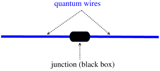
Figure 1: The unit of our quantum device consists of the two quantum wires (blue solid lines) and the junction as the black box.

The combination of these units makes a quantum network. The junction is for controlling the information of qubit. The wires play a role of transporting the information.

We suppose that the energy of our unit has the Hamiltonian, $H_{\mathrm{wires}}+H_{\mathrm{junction}}+H_{\mathrm{interaction}}$, where $H_{\mathrm{wires}}$ is the Hamiltonian for the single electron living in the two wires, $H_{\mathrm{junction}}$ the Hamiltonian for the electron in the junction consisting of a physical object such as a quantum dot, and $H_{\mathrm{interaction}}$ describes the interaction between the wires and the junction. The Hamiltonians $H_{\mathrm{wires}}$ and $H_{\mathrm{junction}}$ should be observables in physics, and therefore, self-adjoint operators in mathematics then. We actually have to determine a concrete physical object for the junction to complete and realize our unit in the quantum engineering. But, in this paper, we regarded the junction as a black box so that the junction has mathematical, physical arbitrariness. Thus, we handled the Hamiltonian $H_{\mathrm{wires}}$ only, but we adopted proper boundary condition between the two wires and the junction instead of considering the Hamiltonian $H_{\mathrm{junction}}$ and the interaction $H_{\mathrm{interaction}}$ so that the Hamiltonian $H_{\mathrm{wires}}$ becomes observable, i.e., self-adjoint. The self-adjointness of the Hamiltonian $H_{\mathrm{wires}}$ is mathematically determined by a boundary condition of the wave functions on which the Hamiltonian $H_{\mathrm{wires}}$ acts. In addition to this, the boundary condition is uniquely determined by the quality and the shape of the boundary of a material of the wires in real physics. Thus, the wave functions have to satisfy the unit’s own specific boundary condition to become the residents of the unit, otherwise they are ejected.

Our one-to-one correspondence formulae show how the Benvegnù and Da̧browski’s four-parameter family are concretely determined. Their four-parameter family shows how the phase factor appears and how the electron spin is affected at the boundary. Since von Neumann’s theory gives the form of the wave functions, we can grasp how they pass through the junction. On the other hand, the boundary which is not characterized by the Benvegnù and Da̧browski’s four-parameter family is the case where the wave functions never infiltrate the junction, which is characterized by the two parameters. As is well known, this case is also important, for instance, to demonstrate the Aharonov-Bohm effect experimentally [33, 25]. Thus, through our observation along with Benvegnù and Da̧browski’s result, we understood that, for the wave functions which pass through the junction, the boundary condition has its own relation between the phase factor and the electron spin. The results may suggest a mathematical possibility of making a device for switching the channel of qubit. There is a case of the two units in Fig.2:

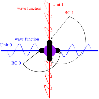
Figure 2: Qubit switch between the two units: The electron wave functions living in quantum wires (blue transversus solid lines) of Unit0 has the boundary condition BC0. If we can change the boundary condition from BC0 to another boundary condition BC1 in a gate (purple disc) connected the junctions, then the electron wave functions have to be residents in the quantum wires (red longitudinal solid lines) of Unit1.

The Unit 0 accepts the wave functions with the boundary condition BC 0 only, and refuses the wave functions with another boundary condition. On the other hand, the Unit 1 welcomes the wave functions with the boundary condition BC 1 different from BC 0, though it rejects the wave functions with the boundary condition BC 0. For instance, as shown in Eqs.(5.2) and (5.3) below, we can use Unit 0 for the channel without spin-flip and Unit 1 for the channel with spin-flip as well as we can use the units for channels for the phase-shifted qubit. Thus, regarding Unit 0 and Unit 1 as a qubit, our switching device in Fig.2 may play a role of quantum state transfer from spintronic qubit. Here we should remember the experimental demonstration of the flying qubit [35], which is realized by the presence of an electron in either channel of the wire of an Aharonov-Bohm ring.

Theorem 4.4 shows the correspondence:

$$U\in U(2) {\longleftrightarrow}$$ is diagonal (4.3)

$$U\in U(2) {\longleftrightarrow} \,\,\,\textrm{(\ref{BC-alpha})}.\qquad\qquad$$ is non-diagonal

Theorem 4.4 assures us that there is no boundary condition which makes a self-adjoint extension but conditions, (4.3) and (4.5). These two conditions make the broad difference: The solitariness in the boundary condition (4.3),

$$(\textrm{left island})\qquad\left\{\begin{array}[]{l}i\rho_{-}\psi_{\uparrow}(-\Lambda)=\psi_{\downarrow}(-\Lambda)\,\,\,\textrm{if\,\,\, $\rho_{-}\in\mathbb{R}$},\\ \psi_{\uparrow}(-\Lambda)=0\,\,\,\textrm{if\,\,\, $\rho_{-}=\infty$},\end{array}\right.$$

and

$$(\textrm{right island})\qquad\left\{\begin{array}[]{l}i\rho_{+}\psi_{\uparrow}(+\Lambda)=\psi_{\downarrow}(+\Lambda)\,\,\,\textrm{if\,\,\, $\rho_{+}\in\mathbb{R}$},\\ \psi_{\uparrow}(+\Lambda)=0\,\,\,\textrm{if\,\,\, $\rho_{+}=\infty$}.\end{array}\right.$$

Both of boundary conditions in the left island and the right one are independent of each other, which says that there is no interchange between the wave functions living in the left island $\Omega_{\Lambda,L}$ and those living in the right island $\Omega_{\Lambda,R}$ because the information of the wave functions never infiltrates the junction. In addition, no special phase factor but $\pm\pi/2$ appears in this boundary condition then.

On the other hand, according to Eq.(15) of Ref.[8] described by the Benvegnù and Da̧browski’s four-parameter family with the representation Proposition 4.7, the boundary condition (4.5) shows how the wave functions living in the left island and the those living in the right island make interchange between each other, and how the electron spin is affected by the phase factor at the boundaries:

$$\left(\begin{array}[]{c}\psi_{\uparrow}(+\Lambda)\\ \psi_{\downarrow}(+\Lambda)\\ \end{array}\right)=\left(\begin{array}[]{c}e^{i\theta}a_{1}\psi_{\uparrow}(-\Lambda)+e^{i(\theta+\pi/2)}a_{2}\psi_{\downarrow}(-\Lambda)\\ e^{i(\theta+\pi/2)}a_{3}\psi_{\uparrow}(-\Lambda)+e^{i\theta}a_{4}\psi_{\downarrow}(-\Lambda)\end{array}\right)$$ (5.1)

for some $a_{j}\in\mathbb{R}$, $j=1,\cdots,4$, with $a_{1}a_{4}+a_{2}a_{3}=1$. The wave function (4.6) determines four parameters $\alpha=(\alpha_{1},\alpha_{2},\alpha_{3},\alpha_{4})\in\mathbb{C}^{4}$ through Eq.(4.7). If $a_{j}\in\mathbb{R}$, $j=1,\cdots,4$, satisfy $a_{1}=a_{4}=0$ and $a_{2}a_{3}=1$, we obtain the boundary condition so that the spin-flip with the phase factor $e^{i(\theta+\pi/2)}$ for an arbitrary $\theta\in[0,2\pi)$ takes place, that is, the up-spin and the down-spin interchange with each other:

$$\left(\begin{array}[]{c}\psi_{\uparrow}(+\Lambda)\\ \psi_{\downarrow}(+\Lambda)\\ \end{array}\right)=e^{i(\theta+\pi/2)}\left(\begin{array}[]{c}a_{2}\psi_{\downarrow}(-\Lambda)\\ a_{3}\psi_{\uparrow}(-\Lambda)\end{array}\right).$$ (5.2)

Meanwhile, if $a_{j}\in\mathbb{R}$, $j=1,\cdots,4$, satisfy $a_{1}a_{4}=1$ and $a_{2}=a_{3}=0$, we obtain the boundary condition so that the phase factor $e^{i\theta}$ appears for an arbitrary $\theta\in[0,2\pi)$ but the spin-flip does not take place:

$$\left(\begin{array}[]{c}\psi_{\uparrow}(+\Lambda)\\ \psi_{\downarrow}(+\Lambda)\\ \end{array}\right)=e^{i\theta}\left(\begin{array}[]{c}a_{1}\psi_{\uparrow}(-\Lambda)\\ a_{4}\psi_{\downarrow}(-\Lambda)\end{array}\right).$$ (5.3)

In Fig.2, for instance, let us employ Eq.(5.3) with $a_{1}=a_{4}=1$ and $\theta=0$ for Unit 0, and Eq.(5.2) with $a_{2}=a_{3}=1$ and $\theta=\,-\pi/2$ for Unit 1, respectively. We set the Pauli-X gate in the disc of junctions. Then, the residence of the wave functions living in Unit 0 is switched to Unit 1 after the Pauli-X gate operation. That is, we have a spin-based switching device for qubit. Thus, there is a possibility that we can use this switching device for quantum state transfer from spintronic qubit regarding Unit 0 and Unit 1 as qubit. In the same way, if we employ Eq.(5.3) with $a_{1}=a_{4}=1$ and $0<\theta<2\pi$ for Unit 1 instead, we can make a phase-based switching device for qubit. This means that we may control the qubit consisting of Unit 0 and Unit 1 through the phase factor $\theta$. We note that both the spin-flip gate operation and the phase-shift gate operation had been demonstrated in the experiment for the spin state of an electron-hole pair in a semiconductor quantum dot [16].

6 Proofs of Main Results

We will give individual proofs of our main results.

6.1 Proof of Proposition 4.1

We now prove Proposition 4.1. Let $\psi={{}^{t}}(\psi_{\uparrow},\psi_{\downarrow})$ be in the deficiency subspace $\mathcal{K}_{\pm}(H_{0})$, i.e., $\psi\in\mathcal{K}_{+}(H_{0})$ or $\psi\in\mathcal{K}_{-}(H_{0})$. Then, since $H_{0}^{*}\psi=\pm i\psi$, Proposition 3.2 gives us the following differential equation:

$$\left(\begin{array}[]{c}\psi_{\uparrow}{\,}^{\prime}\\ \psi_{\downarrow}{\,}^{\prime}\end{array}\right)=\left(\begin{array}[]{cc}0&(\mp 1+im)\\ (\mp 1-im)&0\end{array}\right)\left(\begin{array}[]{c}\psi_{\uparrow}\\ \psi_{\downarrow}\end{array}\right).$$ (6.1)

We note that $\mathcal{K}_{\pm}(H_{0})\subset\mathcal{AC}(\overline{\Omega_{\Lambda}})$. So, according to the general theory of differential equation, every solution $\psi$ of Eq.(6.1) in $\mathcal{AC}(\overline{\Omega_{\Lambda}})$ is respectively written as

$$\left\{\begin{array}[]{l}\psi=c_{L}^{+}\psi_{L}^{+}+c_{R}^{+}\psi_{R}^{+},\,\,\,c_{L}^{+},c_{R}^{+}\in\mathbb{C},\,\,\,\textrm{if $\psi\in\mathcal{K}_{+}(H_{0})$,}\\ \psi=c_{L}^{-}\psi_{L}^{-}+c_{R}^{-}\psi_{R}^{-},\,\,\,c_{L}^{-},c_{R}^{-}\in\mathbb{C},\,\,\,\textrm{if $\psi\in\mathcal{K}_{-}(H_{0})$.}\end{array}\right.$$ (6.2)

It follows from this representation that $n_{\pm}(H_{0})=2$ because the functions $\psi_{L}^{\sharp}$ and $\psi_{R}^{\sharp}$ mutually intersect orthogonally in the Hilbert space $L^{2}(\Omega_{\Lambda})$. The existence of self-adjoint extensions follows from Proposition 2.1.

6.2 Proof of Theorem 4.2

To prove Theorem 4.2 we prepare the following lemma here.

Lemma 6.1

1. Let $a_{1},a_{2},b_{1},b_{2}$ be arbitrary complex numbers.

   1. For every $\rho=(\rho_{+},\rho_{-})$ with $|\rho_{\pm}|<\infty$, there is a wave function $\psi\in D(H_{\rho})$ so that $\psi_{\uparrow}(+\Lambda)=a_{1}$ and $\psi_{\uparrow}(-\Lambda)=a_{2}$.

   2. For every $\rho=(\rho_{+},\rho_{-})$ with $|\rho_{+}|<\infty$ and $\rho_{-}=+\infty$, there is a wave function $\psi\in D(H_{\rho})$ so that $\psi_{\uparrow}(+\Lambda)=a_{1}$ and $\psi_{\downarrow}(-\Lambda)=b_{1}$.

   3. For every $\rho=(\rho_{+},\rho_{-})$ with $\rho_{+}=+\infty$ and $|\rho_{-}|<\infty$, there is a wave function $\psi\in D(H_{\rho})$ so that $\psi_{\uparrow}(-\Lambda)=a_{2}$ and $\psi_{\downarrow}(+\Lambda)=b_{2}$.

   4. For every $\rho=(\rho_{+},\rho_{-})$ with $\rho_{\pm}=+\infty$, there is a wave function $\psi\in D(H_{\rho})$ so that $\psi_{\downarrow}(-\Lambda)=b_{1}$ and $\psi_{\downarrow}(+\Lambda)=b_{2}$.

2. For arbitrary vector ${{}^{t}}(a_{1},a_{2})\in\mathbb{C}^{2}$, there is a wave function $\psi\in D(H_{\alpha})$ so that ${{}^{t}}(\psi_{\uparrow}(-\Lambda),\psi_{\downarrow}(-\Lambda))={{}^{t}}(a_{1},a_{2})$.

Proof:  We embed the function spaces $\mathcal{AC}(\overline{\Omega_{\Lambda,L}})$ and $\mathcal{AC}(\overline{\Omega_{\Lambda,R}})$ in the function space $\mathcal{AC}(\overline{\Omega_{\Lambda}})$ in the following: for every $\psi\in\mathcal{AC}(\overline{\Omega_{\Lambda,L}})$, we expand the function $\psi$ as $\psi(x)=0$ for $x\in\overline{\Omega_{\Lambda,R}}$ and regard the function $\psi$ as the function on $\overline{\Omega_{\Lambda}}$. We employ the same expansion for functions in $\mathcal{AC}(\overline{\Omega_{\Lambda,R}})$.

i) It is not so difficult to show this part. Let $\rho$ be in $\mathbb{R}^{2}$. Fix an arbitrary function $f\in AC^{1}(\overline{\Omega_{\Lambda,R}})$ with $f(+\Lambda)\neq 0$, and take it. For an arbitrary number $a_{1}\in\mathbb{C}$ we define functions $\psi_{R}$ by $\psi_{R}:=(a_{1}/f(+\Lambda))\,{}^{t}\!\left(f,i\rho_{+}f\right)\in\mathcal{AC}(\overline{\Omega_{\Lambda,R}})$. Similarly, take a function $g\in AC^{1}(\overline{\Omega_{\Lambda,L}})$ with $g(-\Lambda)\neq 0$. For an arbitrary number $a_{2}\in\mathbb{C}$ we define functions $\psi_{L}$ by $\psi_{L}:=(a_{2}/g(-\Lambda))\,{}^{t}\!\left(g,i\rho_{-}g\right)\in\mathcal{AC}(\overline{\Omega_{\Lambda,L}})$.

In the case where $|\rho_{\pm}|<\infty$, define a function $\psi\in\mathcal{AC}(\overline{\Omega_{\Lambda}})$ by $\psi:=\psi_{L}+\psi_{R}$. In the case where $|\rho_{+}|<\infty$ and $\rho_{-}=+\infty$, define a function $\psi\in\mathcal{AC}(\overline{\Omega_{\Lambda}})$ by $\psi:=\psi_{R}+(b_{1}/g(-\Lambda))\,{}^{t}\left(0,g\right)$. In the case where $\rho_{+}=+\infty$ and $|\rho_{-}|<\infty$, define a function $\psi\in\mathcal{AC}(\overline{\Omega_{\Lambda}})$ by $\psi:=\psi_{L}+(b_{2}/f(+\Lambda))\,{}^{t}\!\left(0,f\right)$. In the case where $\rho_{\pm}=+\infty$, define a function $\psi\in\mathcal{AC}(\overline{\Omega_{\Lambda}})$ by $\psi:=(b_{1}/g(-\Lambda))\,{}^{t}\!\left(0,g\right)+(b_{2}/f(+\Lambda))\,{}^{t}\!\left(0,f\right)$. Then, we obtain our desired wave function $\psi$.

ii) Take functions $f,g\in AC^{1}(\overline{\Omega_{\Lambda,L}})$ and $h,k\in AC^{1}(\overline{\Omega_{\Lambda,R}})$ with $f(-\Lambda)\neq 0$, $g(-\Lambda)=0$, $h(+\Lambda)\neq 0$, and $k(+\Lambda)\neq 0$. For arbitrary vector ${{}^{t}}(a_{1},a_{2})\in\mathbb{C}^{2}$ we define functions $\varphi_{L}$ and $\varphi_{R}$ by $\varphi_{L}:=(a_{1}/f(-\Lambda))\,{}^{t}\!\left(f,g\right)\in\mathcal{AC}(\overline{\Omega_{\Lambda,L}})$ and $\varphi_{R}:={}^{t}\left((a_{1}\alpha_{1}/h(+\Lambda))h,(a_{1}\alpha_{3}/k(+\Lambda))k\right)\in\mathcal{AC}(\overline{\Omega_{\Lambda,R}})$, respectively. Define the function $\varphi$ by $\varphi:=\varphi_{L}+\varphi_{R}$. Then, we reach the function $\varphi$ satisfying $\varphi\in D(H_{\alpha})$ with $\varphi(-\Lambda)={{}^{t}}(a_{1},0)$. In the same way, we can obtain a function $\phi$ satisfying $\phi\in D(H_{\alpha})$ with $\phi(-\Lambda)={{}^{t}}(0,a_{2})$. Therefore, defining the function $\psi$ by $\psi:=\varphi+\phi$, this function is our desired one.   $\blacksquare$

We here prove Theorem 4.2. Using integration by parts, for every $\psi,\phi\in D(H_{0}^{*})$ we have the following equation:

$$\langle H_{0}^{*}\psi\,|\,\phi\rangle_{L^{2}(\Omega_{\Lambda})\oplus L^{2}(\Omega_{\Lambda})}-\langle\psi\,|\,H_{0}^{*}\phi\rangle_{L^{2}(\Omega_{\Lambda})\oplus L^{2}(\Omega_{\Lambda})}$$

$$= \,-i\bigg{\{}\psi_{\uparrow}(+\Lambda)^{*}\phi_{\downarrow}(+\Lambda)+\psi_{\downarrow}(+\Lambda)^{*}\phi_{\uparrow}(+\Lambda)$$

$$\qquad\quad-\psi_{\uparrow}(-\Lambda)^{*}\phi_{\downarrow}(-\Lambda)-\psi_{\downarrow}(-\Lambda)^{*}\phi_{\uparrow}(-\Lambda)\bigg{\}}.$$

i) We prove our statement in the case where $\rho\in\mathbb{R}^{2}$ only. It is clear that $H_{0}\subset H_{\rho}$.

First up, we show $H_{\rho}\subset H_{\rho}^{*}$. Since $H_{\rho}\subset H_{0}^{*}$, Eq.(6.2) leads to the equation,

$$\langle H_{\rho}\psi\,|\,\phi\rangle_{L^{2}(\Omega_{\Lambda})\oplus L^{2}(\Omega_{\Lambda})}-\langle\psi\,|\,H_{\rho}\phi\rangle_{L^{2}(\Omega_{\Lambda})\oplus L^{2}(\Omega_{\Lambda})}$$

$$= \,-i\bigg{\{}\psi_{\uparrow}(+\Lambda)^{*}(i\rho_{+}\phi_{\uparrow}(+\Lambda))+(i\rho_{+}\psi_{\uparrow}(+\Lambda))^{*}\phi_{\uparrow}(+\Lambda)$$

$$\qquad\quad-\psi_{\uparrow}(-\Lambda)^{*}(i\rho_{-}\phi_{\uparrow}(-\Lambda))-(i\rho_{-}\psi_{\uparrow}(-\Lambda))^{*}\phi_{\uparrow}(-\Lambda)\bigg{\}}=0$$

for every $\psi,\phi\in D(H_{\rho})$. This means that $H_{\rho}$ is symmetric, i.e., $H_{\rho}\subset H_{\rho}^{*}$.

Next, we show $H_{\rho}\supset H_{\rho}^{*}$. Based on Lemma 6.1 (i-1), for arbitrary vector ${{}^{t}}(a_{1},a_{2})\in\mathbb{C}^{2}$, we employ the wave function $\psi\in D(H_{\rho})$ so that $\psi_{\uparrow}(+\Lambda)=a_{1}^{*}$ and $\psi_{\uparrow}(-\Lambda)=a_{2}^{*}$. Using the definition of the adjoint operator, the fact that $H_{\rho}\subset H_{\rho}^{*}\subset H_{0}^{*}$, and Eq.(6.2), we have the equation,

$$0 {=} \langle H_{\rho}\psi\,|\,\phi\rangle_{L^{2}(\Omega_{\Lambda})\oplus L^{2}(\Omega_{\Lambda})}-\langle\psi\,|\,H_{\rho}^{*}\phi\rangle_{L^{2}(\Omega_{\Lambda})\oplus L^{2}(\Omega_{\Lambda})}$$

$${=} \,-i\bigg{\{}a_{1}(\phi_{\downarrow}(+\Lambda)-i\rho_{+}\phi_{\uparrow}(+\Lambda))-a_{2}(\phi_{\downarrow}(-\Lambda)-i\rho_{-}\phi_{\uparrow}(-\Lambda))\bigg{\}}$$

for every $\phi\in D(H_{\rho}^{*})$. Because the complex numbers $a_{1}$ and $a_{2}$ were arbitrarily, we have the equations: $\phi_{\downarrow}(+\Lambda)-i\rho_{+}\phi_{\uparrow}(+\Lambda)=0$ and $\phi_{\downarrow}(-\Lambda)-i\rho_{-}\phi_{\uparrow}(-\Lambda)$ for every $\phi\in D(H_{\rho}^{*})$. These conditions say that $\phi\in D(H_{\rho})$, namely, $D(H_{\rho}^{*})\subset D(H_{\rho})$ and thus $H_{\rho}^{*}\subset H_{\rho}$. Therefore, we have showed that the Dirac operator $H_{\rho}$ is a self-adjoint extension of the minimal Dirac operator: $H_{0}\subset H_{\rho}=H_{\rho}^{*}$.

In the same way, we can prove our statement for the case where $|\rho_{+}|=\infty$ or $|\rho_{-}|=\infty$ with the help of Lemma 6.1 (i-2)–(i-4).

ii) Let us fix an arbitrary vector $\alpha\in\mathbb{C}^{4}$ in the class (4.4). It is clear that $H_{0}\subset H_{\alpha}$. By Eq.(6.2) together with the fact that $H_{\alpha}\subset H_{0}^{*}$, we have the equation,

$$\langle H_{\alpha}\psi\,|\,\phi\rangle_{L^{2}(\Omega_{\Lambda})\oplus L^{2}(\Omega_{\Lambda})}-\langle\psi\,|\,H_{\alpha}\phi\rangle_{L^{2}(\Omega_{\Lambda})\oplus L^{2}(\Omega_{\Lambda})}$$

$${=} \,-i\biggl{\{}(\alpha_{1}^{*}\alpha_{3}+\alpha_{1}\alpha_{3}^{*})\psi_{\uparrow}(-\Lambda)^{*}\phi_{\uparrow}(-\Lambda)+(\alpha_{2}^{*}\alpha_{4}+\alpha_{2}\alpha_{4}^{*})\psi_{\downarrow}(-\Lambda)^{*}\phi_{\downarrow}(-\Lambda)$$

$$\qquad\quad+(\alpha_{1}^{*}\alpha_{4}+\alpha_{2}\alpha_{3}^{*}-1)\psi_{\uparrow}(-\Lambda)^{*}\phi_{\downarrow}(-\Lambda)$$

$$\qquad\qquad+(\alpha_{1}\alpha_{4}^{*}+\alpha_{2}^{*}\alpha_{3}-1)\psi_{\downarrow}(-\Lambda)^{*}\phi_{\uparrow}(-\Lambda)\biggr{\}}=0$$

for every $\psi,\phi\in D(H_{\alpha})$. This means that $H_{\alpha}$ is symmetric, i.e., $H_{\alpha}\subset H_{\alpha}^{*}$.

Based on Lemma 6.1 ii), for arbitrary vector ${{}^{t}}(a_{1},a_{2})\in\mathbb{C}^{2}$, we employ the wave function $\psi\in D(H_{\alpha})$ so that ${{}^{t}}(\psi_{\uparrow}(-\Lambda),\psi_{\downarrow}(-\Lambda))={{}^{t}}(a_{1}^{*},a_{2}^{*})$. Using the definition of the adjoint operator, the fact that $H_{\alpha}\subset H_{\alpha}^{*}\subset H_{0}^{*}$, and Eq.(6.2), we have the equation,

$$0 {=} \langle H_{\alpha}\psi\,|\,\phi\rangle_{L^{2}(\Omega_{\Lambda})\oplus L^{2}(\Omega_{\Lambda})}-\langle\psi\,|\,H_{\alpha}^{*}\phi\rangle_{L^{2}(\Omega_{\Lambda})\oplus L^{2}(\Omega_{\Lambda})}$$

$${=} \,-i\biggl{\{}(\alpha_{1}^{*}\phi_{\downarrow}(+\Lambda)+\alpha_{3}^{*}\phi_{\uparrow}(+\Lambda)-\phi_{\downarrow}(-\Lambda))a_{1}$$

$$\qquad\quad+(\alpha_{2}^{*}\phi_{\downarrow}(+\Lambda)+\alpha_{4}^{*}\phi_{\uparrow}(+\Lambda)-\phi_{\uparrow}(-\Lambda))a_{2}\biggr{\}}$$

for every $\phi\in D(H_{\alpha}^{*})$. Because the complex numbers $a_{1}$ and $a_{2}$ were arbitrarily, we have the equations: $\alpha_{1}^{*}\phi_{\downarrow}(+\Lambda)+\alpha_{3}^{*}\phi_{\uparrow}(+\Lambda)-\phi_{\downarrow}(-\Lambda)=0$ and $\alpha_{2}^{*}\phi_{\downarrow}(+\Lambda)+\alpha_{4}^{*}\phi_{\uparrow}(+\Lambda)-\phi_{\uparrow}(-\Lambda)=0$ for every $\phi\in D(H_{\alpha}^{*})$. We here note that the immediate computation leads to the entries of the inverse boundary matrix as

$$B_{\alpha}^{-1}=\left(\begin{array}[]{cc}\alpha_{4}^{*}&\alpha_{2}^{*}\\ \alpha_{3}^{*}&\alpha_{1}^{*}\end{array}\right)$$

since $\alpha=(\alpha_{1},\alpha_{2},\alpha_{3},\alpha_{4})$ satisfies the conditions of the class (4.4). Hence it follows that $\phi\in D(H_{\alpha})$, namely, $D(H_{\alpha}^{*})\subset D(H_{\alpha})$ and thus $H_{\alpha}^{*}\subset H_{\alpha}$. Therefore, we have showed that the Dirac operator $H_{\alpha}$ is a self-adjoint extension of the minimal Dirac operator: $H_{0}\subset H_{\alpha}=H_{\alpha}^{*}$.

6.3 Proof of Proposition 4.3

First up, we rewrite $SU(2)$ in terms of the electron spin, that is, in terms of the Hamilton quaternion field spanned by the Pauli spin matrices:

Lemma 6.2

The special unitary group $SU(2)$ has the following representation:

$$SU(2)=S\mathbb{H}=\left\{\left(\begin{array}[]{cc}\alpha&-\beta^{*}\\ \beta&\alpha^{*}\end{array}\right)\in\mathbb{H}\,\bigg{|}\,\alpha,\beta\in\mathbb{C},\,\,\,|\alpha|^{2}+|\beta|^{2}=1\right\}.$$

Proof:  In this proof we use the following representation. Introducing the argument $\theta_{j}\in[0,2\pi)$ of each entry $u_{j}$ of the matrix $U\in M_{2}(\mathbb{C})$, we represent $U$ as

$$U=\left(\begin{array}[]{cc}u_{1}&u_{2}\\ u_{3}&u_{4}\end{array}\right)\,\,\,\textrm{with}\,\,\,u_{j}=|u_{j}|e^{i\theta_{j}},\,\,\,j=1,\cdots,4.$$ (6.4)

Let us handle an arbitrary $U\in U(2)$ for a while. The unitarity of $U$ leads to the equations:

$$I_{\mathbb{C}^{2}} =UU^{*}=\left(\begin{array}[]{cc}|u_{1}|^{2}+|u_{2}|^{2}&u_{1}u_{3}^{*}+u_{2}u_{4}^{*}\\ u_{1}^{*}u_{3}+u_{2}^{*}u_{4}&|u_{3}|^{2}+|u_{4}|^{2}\end{array}\right).$$ (6.7)

$$I_{\mathbb{C}^{2}} =U^{*}U=\left(\begin{array}[]{cc}|u_{1}|^{2}+|u_{3}|^{2}&u_{1}^{*}u_{2}+u_{3}^{*}u_{4}\\ u_{1}u_{2}^{*}+u_{3}u_{4}^{*}&|u_{2}|^{2}+|u_{4}|^{2}\end{array}\right).$$ (6.10)

Comparing the diagonal entries in the first row and the first column of both sides of Eq.(6.10), we have the equality:

$$|u_{1}|^{2}+|u_{3}|^{2}=1.$$ (6.11)

In addition, we similarly have the equality, $|u_{1}|^{2}+|u_{2}|^{2}=1$, by Eq.(6.7). Thus, it follows from these two equalities that

$$|u_{2}|=|u_{3}|.$$ (6.12)

In the same way, using the equalities, $|u_{1}|^{2}+|u_{2}|^{2}=1$ and $|u_{2}|^{2}+|u_{4}|^{2}=1$, we reach the equality:

$$|u_{1}|=|u_{4}|.$$ (6.13)

Comparing the off-diagonal entries in the first row and the second column of both sides of in Eq.(6.7), and using Eqs.(6.12) and (6.13), we have the equation,

$$|u_{1}||u_{3}|\left(e^{i(\theta_{1}-\theta_{3})}+e^{i(\theta_{2}-\theta_{4})}\right)=0.$$

Multiplying the both sides of this by $e^{i(\theta_{3}+\theta_{4})}$, we have

$$|u_{1}||u_{3}|\left(e^{i(\theta_{1}+\theta_{4})}+e^{i(\theta_{2}+\theta_{3})}\right)=0.$$ (6.14)

Thus, we have derived the conditions (6.11), (6.12), (6.13), and (6.14) from the condition $U\in U(2)$.

Conversely, it is easy to check that Eqs.(6.11), (6.12), (6.13), and (6.14) bring us to the condition $U\in U(2)$. Consequently, the condition $U\in U(2)$ is equivalent to the conditions (6.11), (6.12), (6.13), and (6.14):

$$U\in U(2)\Longleftrightarrow\textrm{(\ref{eq:5-3-1}), (\ref{eq:5-3-2}), (\ref{eq:5-3-3}), and (\ref{eq:5-3-4})}.$$ (6.15)

Let us consider the case where $U\in SU(2)$ from now on. Then, we have an extra condition:

$$\mathrm{det}\,U=u_{1}u_{4}-u_{2}u_{3}=1.$$ (6.16)

Combining Eq.(6.16) with Eqs.(6.11)–(6.13) leads to the equations,

$$|u_{1}|^{2}+|u_{3}|^{2}=1=u_{1}u_{4}-u_{2}u_{3}=|u_{1}|^{2}e^{i(\theta_{1}+\theta_{4})}-|u_{3}|^{2}e^{i(\theta_{2}+\theta_{3})},$$

which implies that

$$|u_{3}|^{2}\left(1+e^{i(\theta_{2}+\theta_{3})}\right)=|u_{1}|^{2}\left(e^{i(\theta_{1}+\theta_{4})}-1\right).$$ (6.17)

Assume that $u_{1}u_{3}\neq 0$ now. Then, Eq.(6.14) brings us to the equation:

$$e^{i(\theta_{1}+\theta_{4})}+e^{i(\theta_{2}+\theta_{3})}=0.$$ (6.18)

Eqs.(6.17) and (6.18) say that $|u_{3}|^{2}\left(1-e^{i(\theta_{1}+\theta_{4})}\right)=|u_{1}|^{2}\left(e^{i(\theta_{1}+\theta_{4})}-1\right)$. Suppose that $1-e^{i(\theta_{1}+\theta_{4})}\neq 0$ here. Then, the above equation leads to the relation, $|u_{3}|^{2}=\,-|u_{1}|^{2}<0$. This is a contradiction. Thus, by the reductio ad absurdum, we know that $e^{i(\theta_{1}+\theta_{4})}=1$ and therefore $e^{i(\theta_{2}+\theta_{3})}=\,-1$ by Eq.(6.18).

On the other hand, assume that $u_{1}u_{3}=0$. Then, we have the condition, $u_{1}\neq 0$ or $u_{3}\neq 0$, by Eq.(6.11). In the case where $u_{1}\neq 0$, since we have the equality $u_{3}=0$, the equation $e^{i(\theta_{1}+\theta_{4})}=1$ comes up from Eq.(6.17). In the case $u_{3}\neq 0$, similarly, the equation $e^{i(\theta_{2}+\theta_{3})}=\,-1$ is derived from Eq.(6.17). These arguments make us realize that

$$\left\{\begin{array}[]{l}\textrm{if $u_{1}\neq 0$, then $e^{i(\theta_{1}+\theta_{4})}=1$};\\ \textrm{if $u_{3}\neq 0$, then $e^{i(\theta_{2}+\theta_{3})}=\,-1$}.\end{array}\right.$$ (6.19)

In this way, we succeeded in showing that the condition $U\in SU(2)$ implies the conditions (6.11), (6.12), (6.13), (6.14), and the extra condition (6.19).

We here show that adding the condition (6.19) to the conditions (6.11), (6.12), (6.13), and (6.14) completes a necessary and sufficient condition so that $U\in SU(2)$. In the case where $u_{1}u_{3}\neq 0$, we have the equations, $\mathrm{det}\,U=u_{1}u_{4}-u_{2}u_{3}=|u_{1}|^{2}e^{i(\theta_{1}+\theta_{4})}-|u_{3}|^{3}e^{i(\theta_{2}+\theta_{3})}=|u_{1}|^{2}+|u_{3}|^{2}=1$, since $e^{i(\theta_{1}+\theta_{4})}=1$ and $e^{i(\theta_{2}+\theta_{3})}=\,-1$ by the condition (6.19). In the case $u_{1}u_{3}=0$, if $u_{3}=0$ (resp. $u_{1}=0$), then we have the equality, $|u_{1}|=1$ (resp. $|u_{3}|=1$ ) by Eq.(6.11). Thus, we reach the computation, $\mathrm{det}\,U=|u_{1}|^{2}e^{i(\theta_{1}+\theta_{4})}=1$ (resp. $\mathrm{det}\,U=\,-|u_{3}|^{2}e^{i(\theta_{2}+\theta_{3})}=1$ ) by the condition (6.19). Therefore, the condition, $U\in SU(2)$, is equivalent to the conditions, (6.11), (6.12), (6.13), (6.14), and (6.19):

$$U\in SU(2)\Longleftrightarrow\textrm{(\ref{eq:5-3-1}), (\ref{eq:5-3-2}), (\ref{eq:5-3-3}), (\ref{eq:5-3-4}), and (\ref{eq:5-3-7})}.$$ (6.20)

Based on this equivalence (6.20), set our desired complex numbers as $\alpha:=u_{1}$ and $\beta:=u_{3}$, respectively. Then, we have $u_{2}=0=\,-u_{3}^{*}$ if $u_{3}=0$, and $u_{2}=|u_{3}|e^{i\theta_{2}}=\,-|u_{3}|e^{-i\theta_{3}}=\,-u_{3}^{*}$ if $u_{3}\neq 0$, by (6.12) and (6.19). We have $u_{4}=0=u_{1}^{*}$ if $u_{1}=0$, and $u_{4}=|u_{1}|e^{i\theta_{4}}=|u_{1}|e^{-i\theta_{1}}=u_{1}^{*}$ if $u_{1}\neq 0$, by (6.13) and (6.19). Thus, we obtain the statement of our lemma.   $\blacksquare$

Now we prove Proposition 4.3. We use the matrix representation (6.4) again.

In the case where $u_{3}\neq 0$, through the equivalence (6.15), multiplying the both sides of Eq.(6.14) by $|u_{1}|$ gives us the expression $|u_{1}|^{2}(e^{i(\theta_{1}+\theta_{4})}+e^{i(\theta_{2}+\theta_{3})})=0$. Thus, we can compute the determinant of $U$ as

$$\mathrm{det}\,U=u_{1}u_{4}-u_{2}u_{3} = |u_{1}|^{2}e^{i(\theta_{1}+\theta_{4})}-|u_{3}|^{2}e^{i(\theta_{2}+\theta_{3})}$$

$$= \,-(|u_{1}|^{2}+|u_{3}|^{2})e^{i(\theta_{2}+\theta_{3})}=e^{i(\theta_{2}+\theta_{3}+\pi)}.$$

Here we used Eq.(6.11) of the equivalence (6.15), and the equality $e^{i\pi}=\,-1$. Thus, we realize that $e^{-i(\theta_{2}+\theta_{3}+\pi)/2}U\in SU(2)$. Define our desired complex numbers as $\gamma_{1}:=e^{-i(\theta_{2}+\theta_{3}+\pi)/2}u_{1}=e^{-i(\theta_{2}+\theta_{3}+\pi)/2}\alpha$, $\gamma_{2}:=e^{-i(\theta_{2}+\theta_{3}+\pi)/2}u_{3}=e^{-i(\theta_{2}+\theta_{3}+\pi)/2}\beta$, and $\gamma_{3}:=e^{i(\theta_{2}+\theta_{3}+\pi)/2}$, respectively. Then, Lemma 6.2 gives the representation:

$$U=e^{i(\theta_{2}+\theta_{3}+\pi)/2}e^{-i(\theta_{2}+\theta_{3}+\pi)/2}U=\gamma_{3}\left(\begin{array}[]{cc}\gamma_{1}&-\gamma_{2}^{*}\\ \gamma_{2}&\gamma_{1}^{*}\end{array}\right).$$

On the other hand, in the case $u_{3}=0$, we can compute the determinant of $U$ as $\mathrm{det}\,U=e^{i(\theta_{1}+\theta_{4})}$ since we have the value of $|u_{1}|^{2}$ as $|u_{1}|^{2}=1$ by Eq.(6.11) of the equivalence (6.15). Thus, we realize that $e^{-i(\theta_{1}+\theta_{4})/2}U\in SU(2)$. Based on Lemma 6.2, define our desired complex numbers as $\gamma_{1}:=e^{-i(\theta_{1}+\theta_{4})/2}u_{1}=e^{-i(\theta_{1}+\theta_{4})/2}\alpha$, $\gamma_{2}:=e^{-i(\theta_{1}+\theta_{4})/2}u_{3}=e^{-i(\theta_{1}+\theta_{4})/2}\beta$, and $\gamma_{3}:=e^{i(\theta_{1}+\theta_{4})/2}$, respectively. Then, we reach the conclusion,

$$U=e^{i(\theta_{1}+\theta_{4})/2}e^{-i(\theta_{1}+\theta_{4})/2}U=\gamma_{3}\left(\begin{array}[]{cc}\gamma_{1}&-\gamma_{2}^{*}\\ \gamma_{2}&\gamma_{1}^{*}\end{array}\right).$$

These are the construction of the representation in our proposition.

6.4 Proof of Theorem 4.4

Before proving Theorem 4.4, we make a small remark: For every $\psi\in D(H_{U})$, there are $\psi_{0}\in D(H_{0})$ and $c_{L},c_{R}\in\mathbb{C}$ so that

$$\psi=\psi_{0}+c_{L}\psi_{L}^{+}+c_{R}\psi_{R}^{+}+U(c_{L}\psi_{L}^{+}+c_{R}\psi_{R}^{+})$$ (6.21)

by Propositions 2.1 and 4.1 together with Eq.(6.2).

We prove Theorem 4.4 i) here. Let us suppose that $U$ is diagonal. In this case, it is clear that there are complex numbers $\gamma_{L},\gamma_{R}\in\mathbb{C}$ so that

$$U=\left(\begin{array}[]{cc}\gamma_{L}&0\\ 0&\gamma_{R}\end{array}\right),\quad|\gamma_{L}|=|\gamma_{R}|=1,$$

and thus, the operation of the unitary operator $U$ on $\mathcal{K}_{+}(H_{0})$ is determined by $U\psi_{L}^{+}=\gamma_{L}\psi_{L}^{-}$ and $U\psi_{R}^{+}=\gamma_{R}\psi_{R}^{-}$. By Eq.(6.21), we can represent the boundary value $\psi(-\Lambda)$ as

$$\psi(-\Lambda)=c_{L}\psi_{L}^{+}(-\Lambda)+c_{L}\gamma_{L}\psi_{L}^{-}(-\Lambda)=c_{L}Ne^{-\sqrt{1+m^{2}}\,\Lambda}\left(\begin{array}[]{c}1+\gamma_{L}\\ -\mu+\gamma_{L}\mu^{*}\end{array}\right),$$

and the boundary value $\psi(+\Lambda)$ as

$$\psi(+\Lambda)=c_{R}\psi_{R}^{+}(+\Lambda)+c_{R}\gamma_{R}\psi_{R}^{-}(+\Lambda)=c_{R}Ne^{-\sqrt{1+m^{2}}\,\Lambda}\left(\begin{array}[]{c}1+\gamma_{R}\\ \mu-\gamma_{R}\mu^{*}\end{array}\right).$$

We set $\theta_{\mu}$ as $\theta_{\mu}:=\arg\mu$, and so, we have $\mu=e^{i\theta_{\mu}}$. Here $\mu$ was given as $\mu=(1+im)/\sqrt{1+m^{2}}$, and thus, $\cos\theta_{\mu}=1/\sqrt{1+m^{2}}$ and $\sin\theta_{\mu}=m/\sqrt{1+m^{2}}$. We compare the boundary values $\psi_{\uparrow}(-\Lambda)$ and $\psi_{\downarrow}(-\Lambda)$:

In the case where $\gamma_{L}\neq\,-1$, we have

$$\frac{\psi_{\downarrow}(-\Lambda)}{\psi_{\uparrow}(-\Lambda)} {=} \frac{-\mu+\gamma_{L}\mu^{*}}{1+\gamma_{L}}$$

$${=} \frac{(-\mu+\gamma_{L}\mu^{*})(1+\gamma_{L}^{*})}{(1+\gamma_{L})(1+\gamma_{L}^{*})}=\,-\,\frac{\mu-\gamma_{L}\mu^{*}+\gamma_{L}^{*}\mu-\mu^{*}}{2+\gamma_{L}+\gamma_{L}^{*}}$$

$${=} \,-i\frac{\sin(\theta_{\mu}-\theta_{L})+\sin\theta_{\mu}}{1+\cos\theta_{L}}=i\left(\cos\theta_{\mu}\tan\frac{\theta_{L}}{2}-\sin\theta_{\mu}\right).$$

The value of $\cos\theta_{\mu}\tan(\theta_{L}/2)-\sin\theta_{\mu}$ runs over the whole $\mathbb{R}$ when the angular $\theta_{L}$ runs over $[0,2\pi)\setminus\{\pi\}$, and then, the correspondence $[0,2\pi)\setminus\{\pi\}\ni\theta_{L}\longrightarrow\rho_{-}\in\mathbb{R}$ makes the one-to-one correspondence. On the other hand, in the case where $\gamma_{L}=\,-1$, we have $\psi_{\uparrow}(-\Lambda)=0$ and $\psi_{\downarrow}(-\Lambda)=\,-c_{L}Ne^{-\sqrt{1+m^{2}}\Lambda}(\mu+\mu^{*})$.

Similarly, compare the boundary values $\psi_{\uparrow}(+\Lambda)$ and $\psi_{\downarrow}(+\Lambda)$: In the case where $\gamma_{R}\neq\,-1$, we have

$$\frac{\psi_{\downarrow}(+\Lambda)}{\psi_{\uparrow}(+\Lambda)}=\frac{\mu-\gamma_{R}\mu^{*}}{1+\gamma_{R}}=i\left(-\cos\theta_{\mu}\tan\frac{\theta_{R}}{2}+\sin\theta_{\mu}\right).$$

The correspondence $[0,2\pi)\setminus\{\pi\}\ni\theta_{R}\longrightarrow\rho_{+}\in\mathbb{R}$ makes the one-to-one correspondence. In the case where $\gamma_{R}=\,-1$, we have $\psi_{\uparrow}(+\Lambda)=0$ and $\psi_{\downarrow}(+\Lambda)=c_{R}Ne^{-\sqrt{1+m^{2}}\Lambda}(\mu+\mu^{*})$.

Therefore, we realize that the condition, $D(H_{\rho})=D(H_{U})$, is equivalent to the correspondence: $i\rho_{-}=\psi_{\downarrow}(-\Lambda)/\psi_{\uparrow}(-\Lambda)$ for $\gamma_{L}\neq\,-1$ and $\rho_{-}=|\psi_{\downarrow}(-\Lambda)/\psi_{\uparrow}(-\Lambda)|=+\infty$ for $\gamma_{L}=\,-1$, and $i\rho_{+}=\psi_{\downarrow}(+\Lambda)/\psi_{\uparrow}(+\Lambda)$ for $\gamma_{R}\neq\,-1$ and $\rho_{+}=|\psi_{\downarrow}(+\Lambda)/\psi_{\uparrow}(+\Lambda)|=+\infty$ for $\gamma_{R}=\,-1$, which gives our desired correspondence.

We prove Theorem 4.4 ii) now. First up, Proposition 4.3 gives the representation of $U$: there are complex numbers $\gamma_{1},\gamma_{2},\gamma_{3}\in\mathbb{C}$ so that

$$U=\gamma_{3}\left(\begin{array}[]{cc}\gamma_{1}&-\gamma_{2}^{*}\\ \gamma_{2}&\gamma_{1}^{*}\end{array}\right)\,\,\,\textrm{with}\,\,\,|\gamma_{1}|^{2}+|\gamma_{2}|^{2}=|\gamma_{3}|=1,\,\gamma_{2}\neq 0.$$

Here the fact, $\gamma_{2}\neq 0$, comes from the assumption that $U$ is non-diagonal. Thus, the operation of $U$ on $\mathcal{K}_{+}(H_{0})$ is determined by $U\psi_{L}^{+}=\gamma_{1}\gamma_{3}\psi_{L}^{-}-\gamma_{2}^{*}\gamma_{3}\psi_{R}^{-}$ and $U\psi_{R}^{+}=\gamma_{2}\gamma_{3}\psi_{L}^{-}+\gamma_{1}^{*}\gamma_{3}\psi_{R}^{-}$. Using Eq.(6.21), we can compute individual boundary values $\psi(-\Lambda)$ and $\psi(+\Lambda)$ as

$$\psi(-\Lambda) {=} c_{L}\psi_{L}^{+}(-\Lambda)+c_{L}\gamma_{1}\gamma_{3}\psi_{L}^{-}(-\Lambda)+c_{R}\gamma_{2}\gamma_{3}\psi_{L}^{-}(-\Lambda)$$

$${=} Ne^{-\sqrt{1+m^{2}}\Lambda}\left(\begin{array}[]{cc}1+\gamma_{1}\gamma_{3}&\gamma_{2}\gamma_{3}\\ -\mu+\gamma_{1}\gamma_{3}\mu^{*}&\gamma_{2}\gamma_{3}\mu^{*}\end{array}\right)\left(\begin{array}[]{c}c_{L}\\ c_{R}\end{array}\right)$$

and

$$\psi(+\Lambda) {=} c_{R}\psi_{R}^{+}(+\Lambda)-c_{L}\gamma_{2}^{*}\gamma_{3}\psi_{R}^{-}(+\Lambda)+c_{R}\gamma_{1}^{*}\gamma_{3}\psi_{R}^{-}(+\Lambda)$$

$${=} Ne^{-\sqrt{1+m^{2}}\Lambda}\left(\begin{array}[]{cc}-\gamma_{2}^{*}\gamma_{3}&1+\gamma_{1}^{*}\gamma_{3}\\ \gamma_{2}^{*}\gamma_{3}\mu^{*}&\mu-\gamma_{1}^{*}\gamma_{3}\mu^{*}\end{array}\right)\left(\begin{array}[]{c}c_{L}\\ c_{R}\end{array}\right).$$

We remember that $\gamma_{2}\neq 0$ and $\gamma_{3}\neq 0$, and then,

$$\mathrm{det}\,\left(\begin{array}[]{cc}1+\gamma_{1}\gamma_{3}&\gamma_{2}\gamma_{3}\\ -\mu+\gamma_{1}\gamma_{3}\mu^{*}&\gamma_{2}\gamma_{3}\mu^{*}\end{array}\right)=\gamma_{2}\gamma_{3}(\mu+\mu^{*})=\frac{2\gamma_{2}\gamma_{3}}{\sqrt{1+m^{2}}}\neq 0.$$

Thus, noting $\gamma_{3}^{-1}=\gamma_{3}^{*}$, we can compute the following inverse matrix:

$$\left(\begin{array}[]{cc}1+\gamma_{1}\gamma_{3}&\gamma_{2}\gamma_{3}\\ -\mu+\gamma_{1}\gamma_{3}\mu^{*}&\gamma_{2}\gamma_{3}\mu^{*}\end{array}\right)^{-1}=\frac{1}{\gamma_{2}(\mu+\mu^{*})}\left(\begin{array}[]{cc}\gamma_{2}\mu^{*}&-\gamma_{2}\\ \gamma_{3}^{*}\mu-\gamma_{1}\mu^{*}&\gamma_{1}+\gamma_{3}^{*}\end{array}\right).$$

Thus, define a $2\times 2$ matrix $V$ by

$$V\equiv\left(\begin{array}[]{cc}v_{1}&v_{2}\\ v_{3}&v_{4}\\ \end{array}\right):=\left(\begin{array}[]{cc}-\gamma_{2}^{*}\gamma_{3}&1+\gamma_{1}^{*}\gamma_{3}\\ \gamma_{2}^{*}\gamma_{3}\mu^{*}&\mu-\gamma_{1}^{*}\gamma_{3}\mu^{*}\end{array}\right)\left(\begin{array}[]{cc}1+\gamma_{1}\gamma_{3}&\gamma_{2}\gamma_{3}\\ -\mu+\gamma_{1}\gamma_{3}\mu^{*}&\gamma_{2}\gamma_{3}\mu^{*}\end{array}\right)^{-1}.$$

Then, we have

$$V=\frac{\sqrt{1+m^{2}}}{\gamma_{2}}\left(\begin{array}[]{cc}i\left\{\Im(\gamma_{1}^{*}\mu)+\Im(\gamma_{3}^{*}\mu)\right\}&\Re\gamma_{1}+\Re\gamma_{3}\\ -\Re\gamma_{1}+\Re(\gamma_{3}^{*}\mu^{2})&i\left\{\Im(\gamma_{1}\mu)+\Im(\gamma_{3}^{*}\mu)\right\}\end{array}\right).$$

Thus, we reach the boundary condition: $\psi(+\Lambda)=V\psi(-\Lambda)$ for every $\psi\in D(H_{U})$. We set $v_{j}^{\prime}$ as $v_{j}^{\prime}:=i(\gamma_{2}/|\gamma_{2}|)v_{j}$, $j=1,\cdots,4$, and then, we have $v_{j}^{\prime}{v_{k}^{\prime}}^{*}=v_{j}v_{k}^{*}$. Then, $v_{1}^{\prime}$ and $v_{4}^{\prime}$ are real numbers, and $v_{2}^{\prime}$ and $v_{3}^{\prime}$ are purely imaginary numbers, which implies the relations: $\Re(v_{1}v_{2}^{*})=\Re(v_{1}^{\prime}{v_{2}^{\prime}}^{*})=0$, $\Re(v_{1}v_{3}^{*})=\Re(v_{1}^{\prime}{v_{3}^{\prime}}^{*})=0$, $\Re(v_{2}v_{4}^{*})=\Re(v_{2}^{\prime}{v_{4}^{\prime}}^{*})=0$, and $\Re(v_{3}v_{4}^{*})=\Re(v_{3}^{\prime}{v_{4}^{\prime}}^{*})=0$. So, we have confirmed the first part of conditions of the class (4.4). We check the last two conditions of the class (4.4): The immediate computation easily bring us to $v_{1}v_{4}^{*}+v_{2}v_{3}^{*}=1$ using $|\gamma_{1}|^{2}+|\gamma_{2}|^{2}=1$. We here note that $v_{k}^{*}=v_{k}(\gamma_{2}/\gamma_{2}^{*})$, $k=2,3$, which implies $v_{2}v_{3}^{*}=v_{2}\{v_{3}(\gamma_{2}/\gamma_{2}^{*})\}=\{v_{2}(\gamma_{2}/\gamma_{2}^{*})\}v_{3}=v_{2}^{*}v_{3}^{*}$. Thus, we have $v_{1}v_{4}^{*}+v_{2}^{*}v_{3}=v_{1}v_{4}^{*}+v_{2}v_{3}^{*}=1$. Therefore, we can conclude from the above argument that the vector $v=(v_{1},v_{2},v_{3},v_{4})\in\mathbb{C}^{4}$ is in the class (4.4), and then, $V=B_{v}$. Therefore, the condition, $D(H_{\alpha})=D(H_{U})$, is equivalent to the correspondence $\alpha=v$. We accomplished the proof of the part ii).

6.5 Proof of Proposition 4.7

We denote by $\mathcal{A}_{0}$ the set on the right hand side of our desired representation. It is evident that $\mathcal{A}_{0}\subset\mathcal{A}$. So, the only thing we have to do is that we show $\mathcal{A}\subset\mathcal{A}_{0}$. For every $B_{\alpha}\in\mathcal{A}$, set $\theta_{j}$ as $\theta_{j}=\arg\alpha_{j}$. Since the vector $\alpha$ is in the class (4.4), $\alpha_{1}\alpha_{2}^{*}$, $\alpha_{1}\alpha_{3}^{*}$, $\alpha_{2}\alpha_{4}^{*}$, and $\alpha_{3}\alpha_{4}^{*}$ are purely imaginary numbers. Moreover, the last condition of the class (4.4) says that $\alpha_{2}\alpha_{3}^{*}=1-\alpha_{1}\alpha_{4}^{*}=\alpha_{2}^{*}\alpha_{3}$. That is, $\alpha_{2}\alpha_{3}^{*}$ is a real number. Thus, it follows from the last condition, that $\alpha_{1}\alpha_{4}^{*}$ is also a real number, and $\alpha_{1}\neq 0$ or $\alpha_{3}\neq 0$. In the case where $\alpha_{1}\neq 0$, setting $\theta\in[0,2\pi)$, and $a_{1},a_{2},a_{3},a_{4}\in\mathbb{R}$ as $\theta:=\arg(\alpha_{1}/|\alpha_{1}|)$, $a_{1}:=|\alpha_{1}|$, $a_{2}:=(\alpha_{1}\alpha_{2}^{*})^{*}/i|\alpha_{1}|$, $a_{3}:=(\alpha_{1}\alpha_{3}^{*})^{*}/i|\alpha_{1}|$, and $a_{4}:=(\alpha_{1}\alpha_{4}^{*})^{*}/|\alpha_{1}|$, we immediately obtain the representation of $B_{\alpha}$ in $\mathcal{A}_{0}$. In the case $\alpha_{1}=0$, we only have to set $\theta\in[0,2\pi)$, and $a_{1},a_{2},a_{3},a_{4}\in\mathbb{R}$ by $\theta:=\arg(-i\alpha_{3}/|\alpha_{3}|)$, $a_{1}:=i\alpha_{1}\alpha_{3}^{*}/|\alpha_{3}|$, $a_{2}:=\alpha_{2}\alpha_{3}^{*}/|\alpha_{3}|$, $a_{3}:=|\alpha_{3}|$, and $a_{4}:=i(\alpha_{3}\alpha_{4}^{*})^{*}/|\alpha_{3}|$, respectively, and then, we reach our desired fact $B_{\alpha}\in\mathcal{A}_{0}$. Thus, the two cases imply that $\mathcal{A}\subset\mathcal{A}_{0}$. Therefore, we can conclude the proof of the equality, $\mathcal{A}=\mathcal{A}_{0}$.

6.6 Proof of Proposition 4.6

We prove Proposition 4.6 here. First up, it immediately follows from the definition of $\gamma_{1}$, $\gamma_{2}$, and $\Gamma_{0}$ that $|\gamma_{1}|^{2}+|\gamma_{2}|^{2}=1$. We here remark that this equation gives us the equation,

$$1=\Gamma_{0}^{2} \Bigl{[}\frac{4}{1+m^{2}}+\sum_{j=1}^{4}|\alpha_{j}|^{2}-2\Re(\mu^{*}\alpha_{1}\alpha_{2}^{*})+2\Re(\mu^{*}\alpha_{1}\alpha_{3}^{*})-2\Re(\mu^{*2}\alpha_{1}\alpha_{4}^{*})$$ (6.24)

$$\quad-2\Re(\alpha_{2}\alpha_{3}^{*})+2\Re(\mu\alpha_{2}^{*}\alpha_{4})-2\Re(\mu\alpha_{3}^{*}\alpha_{4})\Bigr{]}.$$

Next, we show $|\gamma_{3}|=1$. It is easy to check the equations,

$$\Re(\mu\alpha_{1}\alpha_{j}^{*})=\,-\Re(\mu^{*}\alpha_{1}\alpha_{j}^{*})=\frac{m}{\sqrt{1+m^{2}}}a_{1}a_{j},\quad j=2,3,$$

$$\Re(\mu^{*}\alpha_{j}^{*}\alpha_{4})=\,-\Re(\mu\alpha_{j}^{*}\alpha_{4})=\,-\,\frac{m}{\sqrt{1+m^{2}}}a_{j}a_{4},\quad j=2,3,$$

$$\Re(\mu^{*2}\alpha_{j}\alpha_{k}^{*})=\frac{1-m^{2}}{1+m^{2}}\Re(\alpha_{j}\alpha_{k}^{*})=\frac{1-m^{2}}{1+m^{2}}a_{j}a_{k},\quad(j,k)=(1,4),(2,3),$$

by Proposition 4.7. By using these equations together with

$$\frac{1\mp m^{2}}{1\pm m^{2}}=\frac{2}{1\pm m^{2}}\,-1,$$

we have

$$|\gamma_{3}|^{2} {=} \Gamma_{0}^{2}\Bigl{[}\sum_{j=1}^{4}|\alpha_{j}|^{2}+2\Re(\mu\alpha_{1}\alpha_{2}^{*})+2\Re(\mu^{*}\alpha_{1}\alpha_{3}^{*})+2\Re(\alpha_{1}\alpha_{4}^{*})+2\Re(\mu^{*2}\alpha_{2}\alpha_{3}^{*})$$

$$\qquad+2\Re(\mu\alpha_{2}^{*}\alpha_{4})+2\Re(\mu^{*}\alpha_{3}^{*}\alpha_{4})\Bigr{]}$$

$${=} \textrm{right hand side of (\ref{eq:inv-1})}.$$

Thus, we have $|\gamma_{3}|=1$, and then, we reach

$$U=\gamma_{3}\left(\begin{array}[]{cc}\gamma_{1}&-\gamma_{2}^{*}\\ \gamma_{2}&\gamma_{1}^{*}\end{array}\right)\in U(1)S\mathbb{H}=U(2).$$

Thus, what we have to show is that every $\psi\in D(H_{U})$ satisfies the boundary condition (4.5). Insert the boundary values $\psi_{\sharp}(+\Lambda)$ and $\psi_{\sharp}(-\Lambda)$ with expressions,

$$\left\{\begin{array}[]{l}\psi_{\sharp}(+\Lambda)=c_{R}\psi_{R\sharp}^{+}(+\Lambda)-c_{L}\gamma_{3}\gamma_{2}^{*}\psi_{R\sharp}^{-}(+\Lambda)+c_{R}\gamma_{3}\gamma_{1}^{*}\psi_{R\sharp}^{-}(+\Lambda),\\ \psi_{\sharp}(-\Lambda)=c_{L}\psi_{L\sharp}^{+}(-\Lambda)+c_{L}\gamma_{3}\gamma_{1}\psi_{L\sharp}^{-}(-\Lambda)+c_{R}\gamma_{3}\gamma_{2}\psi_{L\sharp}^{-}(-\Lambda),\end{array}\right.\sharp=\uparrow,\downarrow,$$

into the boundary conditions,

$$\left\{\begin{array}[]{l}\psi_{\uparrow}(+\Lambda)=\alpha_{1}\psi_{\uparrow}(-\Lambda)+\alpha_{2}\psi_{\downarrow}(-\Lambda),\\ \psi_{\downarrow}(+\Lambda)=\alpha_{3}\psi_{\uparrow}(-\Lambda)+\alpha_{4}\psi_{\downarrow}(-\Lambda).\end{array}\right.$$

Then, by using the arbitrariness of the coefficients $c_{L}$ and $c_{R}$ in $D(H_{U})$ and noting the fact $\gamma_{3}^{-1}=\gamma_{3}^{*}$, we can show that the condition $D(H_{U})=D(H_{\alpha})$ is equivalent to the system of the following system of equations:

$$(\alpha_{1}+\mu^{*}\alpha_{2})\gamma_{1}+\gamma_{2}^{*}=\gamma_{3}^{*}(-\alpha_{1}+\mu\alpha_{2}),$$ (6.25)

$$(\alpha_{1}+\mu^{*}\alpha_{2})\gamma_{2}-\gamma_{1}^{*}=\gamma_{3}^{*},$$ (6.26)

$$(\alpha_{3}+\mu^{*}\alpha_{4})\gamma_{1}-\mu^{*}\gamma_{2}^{*}=\gamma_{3}^{*}(-\alpha_{3}+\mu\alpha_{4}),$$ (6.27)

$$(\alpha_{3}+\mu^{*}\alpha_{4})\gamma_{2}+\mu^{*}\gamma_{1}^{*}=\mu\gamma_{3}^{*}.$$ (6.28)

Then, we can show that our $(\gamma_{1},\gamma_{2},\gamma_{3})$ is a solution of this system of equations:

Noting $\mu+\mu^{*}=2/\sqrt{1+m^{2}}$ and $a_{1}a_{4}+a_{2}a_{3}=1$, we have $\mu a_{1}a_{4}+\mu^{*}a_{2}a_{3}=2/\sqrt{1+m^{2}}-\mu^{*}a_{1}a_{4}-\mu a_{2}a_{3}$. Thus, we realize that our $\gamma_{1},\gamma_{2},\gamma_{3}$ satisfy (6.25) as

$$(\alpha_{1}+\mu^{*}\alpha_{2})\gamma_{1}+\gamma_{2}^{*} {=} ie^{i\theta}\Gamma_{0}\Bigl{[}-\mu^{*}a_{1}^{2}+i(1-\mu^{*2})a_{1}a_{2}-ia_{1}a_{3}-\mu^{*}a_{1}a_{4}$$

$$\qquad\qquad-\mu^{*}a_{2}^{2}-\mu a_{2}a_{3}+ia_{2}a_{4}\Bigr{]}$$

$${=} \gamma_{3}^{*}(-\alpha_{1}+\mu\alpha_{2}).$$

Using $\mu\mu^{*}=1$ and $\mu^{*2}=2\mu^{*}/\sqrt{1+m^{2}}-1$, we can show that our $\gamma_{1},\gamma_{2},\gamma_{3}$ satisfy (6.26) as

$$(\alpha_{1}+\mu^{*}\alpha_{2})\gamma_{2}-\gamma_{1}^{*}=\Gamma_{0}\left(i\mu^{*}a_{1}-\mu^{*2}a_{2}-a_{3}+i\mu^{*}a_{4}\right)=\gamma_{3}^{*}.$$

Combining $\mu^{*2}=2\mu^{*}/\sqrt{1+m^{2}}-1$ and $a_{1}a_{4}+a_{2}a_{3}=1$, we have $-\mu^{*2}a_{1}a_{4}-a_{2}a_{3}=a_{1}a_{4}^{*}+\mu^{*2}a_{2}a_{3}-2\mu^{*}/\sqrt{1+m^{2}}$. Using this equation and $\mu\mu^{*}=1$, we can show that our $\gamma_{1},\gamma_{2},\gamma_{3}$ satisfy (6.27) as

$$(\alpha_{3}+\mu^{*}\alpha_{4})\gamma_{1}-\mu^{*}\gamma_{2}^{*} {=} i\Gamma_{0}e^{i\theta}\Bigl{[}-i\mu^{*}a_{1}a_{3}+a_{1}a_{4}+\mu^{*2}a_{2}a_{3}+i\mu^{*}a_{2}a_{4}$$

$$\qquad\qquad+a_{3}^{2}+i(\mu-\mu^{*})a_{3}a_{4}+a_{4}^{2}\Bigr{]}$$

$${=} \gamma_{3}^{*}(-\alpha_{3}+\mu\alpha_{4}).$$

Using $\mu\mu^{*}=1$ and $\mu+\mu^{*}=2/\sqrt{1+m^{2}}$, we know that our $\gamma_{1},\gamma_{2},\gamma_{3}$ satisfy (6.28) as

$$(\alpha_{3}+\mu^{*}\alpha_{4})\gamma_{2}+\mu^{*}\gamma_{1}^{*}=\Gamma_{0}\left(ia_{1}-\mu^{*}a_{2}-\mu a_{3}+ia_{4}\right)=\mu\gamma_{3}^{*}.$$

Therefore, consequently, we can complete the proof of our proposition.

7 Conclusion

We have proved that all the boundary conditions of wave functions of our Dirac particle are completely classified into the two types. For the case where the electron’s wave functions do not pass through the junction, their boundary condition can be described by two parameters, $\gamma_{L},\gamma_{R}\in\mathbb{C}$ with $|\gamma_{L}|=|\gamma_{R}|=1$, determined by von Neumann’s theory. In the case where the wave functions do pass through the junction, the boundary condition is described by Benvegnù and Da̧browski’s four-parameter family, and then, their four parameters can actually be described by three parameters, $\gamma_{1},\gamma_{2},\gamma_{3}\in\mathbb{C}$ with $|\gamma_{1}|^{2}+|\gamma_{2}|^{2}=|\gamma_{3}|=1$ and $\gamma_{2}\neq 0$, determined by von Neumann’s theory. These results stem from our one-to-one correspondence formulae, Eqs.(4.7) and (4.11) with Propositions 4.3 and 4.7.

Let us make small two remarks at the tail end of this paper. Using our method, we can completely classify the boundary conditions of all self-adjoint extensions of the minimal Schrödinger operator, too [19]. In the Dirac operator’s case, there is no effect of the length of junction in the boundary condition. However, in the Schrödinger operator’s case, we can find it in the boundary condition. We have not understand any strictly physical reason why the Schrödinger particle feels the length $2\Lambda$ of the junction, but the Dirac particle does not. We conjecture that the speed of the particle is concerned with the reason.

References

• [1] S. Albeverio, F. Gesztesy, R. Høgh-Krohn, and H. Holden, Solvable models in quantum mechanics, Springer, New York, 1988.
• [2] V. Alonso and S. De Vincenzo, Delta-type Dirac point interactions and their nonrelativistic limits, Int. J. Math. Phys., 39 (2000), 1483.
• [3] A. F. Andreev, Thermal conductivity of the intermediate state of superconductors., Sov. Phys. JETP, 19 (1964), 1228.
• [4] A. F. Andreev, Thermal conductivity of the intermediate state of superconductors. II, Sov. Phys. JETP, 20 (1965), 1490.
• [5] D. D. Awschalom, M. E. Flatté, and N. Samarth, Spintronics, Scientific American, 286 (2002), 67.
• [6] J. Behrndt, M. Malamud, and H. Neidhardt, Scattering matrices and Weyl functions, Proc. London Math. Soc., 97 (2008), 568.
• [7] J. Behrndt, H. Neidhardt, E. R. Racec, P. N. Racec, U. Wulf, On Eisenbud’s and Wigner’s R-matrix: A general approach, J. Differ. Equations, 244 (2008), 2545.
• [8] S. Benvegnù and L. Da̧browski, Relativistic point interaction, Lett. Math. Phys., 30 (1994), 159.
• [9] J. Berezovsky, O. Gywat, F. Meier, D. Battaglia, X. Peng, and D. D. Awschalom, Initialization and read-out of spins in coupled core-shell quantum dots, Nature Physics, 2 (2006), 831.
• [10] J. F. Brasche, M. Malamud, and H. Neidhardt, Weyl function and spectral properties of self-adjoint extensions, Integr. Equ. Oper. Theo., 43 (2002), 264.
• [11] J. Brüning, V. Geyler, and K. Pankrashkin, Spectra of self-adjoint extensions and applications to solvable Schrödinger operators, Rev. Math. Phys., 20 (2008), 1.
• [12] G. Burkard, Spin qubits: Connect the dots, Nature Physics, 2 (2006), 807.
• [13] R. Carlone, M. Malamud, and A. Posilicano, On the spectral theory of Gesztesy-Šeba realizations of $1$-$D$ Dirac operators with point interactions on a discrete set, arXiv:1302.5044v1.
• [14] F. Dominguez-Adame and E. Marcia, Bound states and confining properties of rel. point interaction potentials, J. Phys. A, 22 (1989), L419.
• [15] Y. Furuhashi, M. Hirokawa, K. Nakahara, and Y. Shikano, Role of a phase factor in the boundary condition of a one-dimensional junction, J. Phys. A: Math. Theo., 43 (2010), 354010.
• [16] A. B. Giroday, A. J. Bennett, M. A. Pooley, R. M. Stevenson, N. Sköld, R. B. Patel, I. Farrer, D. A. Ritchie, and A. J. Shields, All-electrical coherent control of the exciton states in a single quantum dot, Phys. Rev. B, 82 (2010), 241301.
• [17] S. Hermelin, S. Takada, M. Yamamoto, S. Tarucha, A. D. Wieck, L. Saminadayar, C. Bäuerle, and T. Meunier, Electrons surfing on a sound wave as a platform for quantum optics with flying electrons, Nature, 477 (2011), 435.
• [18] M. Hirokawa, Canonical quantization on a doubly connected space and the Aharonov-Bohm phase, J. Funct. Anal., 174 (2000), 322.
• [19] M. Hirokawa and T. Kosaka, One-dimensional tunnel-junction formula for Schrödinger particle, arXiv:0759041v1.
• [20] R. J. Hughes, Relativistic point interactions: Approximation by smooth potentials, Rep. Math. Phys., 39 (1997), 425.
• [21] M. N. Leuenberger, D. Loss, M. Poggio, and D. D. Awschalom, Quantum information processing with large nuclear spins in GaAs semiconductors, Phys. Rev. Lett., 89 (2002), 207601.
• [22] M. N. Leuenberger, M. E. Flatté, and D. D. Awschalom, Teleportation of electronic many-qubit states encoded in the electron spin of quantum dots via single photons, Phys. Rev. Lett., 94 (2005), 107401.
• [23] D. Loss and D. P. DiVincenzo, Quantum computation with quantum dots, Phys. Rev. A, 57 (1998), 120.
• [24] R. P. G. McNeil, M. Kataoka, C. J. B. Ford, C. H. W. Barnes, D. Anderson, G. A. C. Jones, I. Farrer, and D. A. Ritchie, On-demand single-electron transfer between distant quantum dots, Nature, 477 (2011), 439.
• [25] N. Osakabe, T. Matsuda, T. Kawasaki, J. Endo, A. Tonomura, S. Yano, and H. Yamada, Experimental confirmation of Aharonov-Bohm effect using a toroidal magnetic field confined by a superconductor, Phys. Rev. A, 34 (1986), 815.
• [26] S. Pedersen and F. Tian, Momentum operators in the unit square, Integr. Equ. Oper. Theo., 77 (2013), 57.
• [27] M. Reed and B. Simon, Methods of Modern Mathematical Physics II. Fourier Analysis, Self-Adjointness, Academic Press, San Diego, 1975.
• [28] T. S. Santos, J. S. Lee, P. Migdal, I. C. Lekshmi, B. Satpati, and J. S. Moodera, Room-temperature tunnel magnetoresistance and spin-polarized tunneling through an organic semiconductor barrier, Phys. Rev. Lett., 98 (2007), 016601.
• [29] J. J. H. M. Schoonus, P. G. E. Lumens, W. Wagemans, J. T. Kohlhepp, P. A. Bobbert, H. J. M. Swagten, and B. Koopmans, Magnetoresistance in hybrid organic spin valves at the onset of multiple-step tunneling, Phys. Rev. Lett., 103 (2009), 146601.
• [30] P. Šeba, Klein’s paradox and the relativistic point interaction, Lett. Math. Phys., 18 (1989), 77.
• [31] Y. Shikano and M. Hirokawa, Boundary conditions in one-dimensional tunneling junction, J. Phys.: Conference Series, 302 (2011), 012044.
• [32] A. Tokuno, M. Oshikawa, and E. Demler, Dynamics of one-dimensional Bose liquids: Andreev-like reflection at Y-junctions and the absence of the Aharonov-Bohm effect, Phys. Rev. Lett., 100 (2008), 140402.
• [33] A. Tonomura, N. Osakabe, T. Matsuda, T. Kawasaki, and J. Endo, Evidence for Aharonov-Bohm effect with magnetic field completely shielded from electron wave, Phys. Rev. Lett., 56 (1986), 792.
• [34] J. Weidmann, Linear Operators in Hilbert Spaces, Springer-Verlag, New York, 1980.
• [35] M. Yamamoto, S. Takada, C. Bäuerle, K. Watanabe, A. D. Wieck, and S. Tarucha, Electrical control of a solid-state flying qubit, Nature Nanotechnology, 7 (2012), 247.
• [36] X. Zhang, S. Mizukami, T. Kubota, Q. Ma, M. Oogane, H. Naganuma, Y. Ando, and T. Miyazaki, Observation of a large spin-dependent transport length in organic spin valves at room temperature, Nature Communications, 4 (2013), 1392.