Order-by-disorder in classical oscillator systems
Abstract
We consider classical nonlinear oscillators on hexagonal lattices. When the coupling between the elements is repulsive, we observe coexisting states, each one with its own basin of attraction. These states differ by their degree of synchronization and by patterns of phase-locked motion. When disorder is introduced into the system by additive or multiplicative Gaussian noise, we observe a non-monotonic dependence of the degree of order in the system as a function of the noise intensity: intervals of noise intensity with low synchronization between the oscillators alternate with intervals where more oscillators are synchronized. In the latter case, noise induces a higher degree of order in the sense of a larger number of nearly coinciding phases. This order-by-disorder effect is reminiscent to the analogous phenomenon known from spin systems. Surprisingly, this non-monotonic evolution of the degree of order is found not only for a single interval of intermediate noise strength, but repeatedly as a function of increasing noise intensity. We observe noise-driven migration of oscillator phases in a rough potential landscape.
pacs:
05.45.Xt, 05.40.Ca, 64.60.aqI Introduction
The so-called order-by-disorder effect is usually discussed in different contexts of spin models. The notion refers to the frequently found situation in which the ground state is degenerate due to the competition among the interactions, and this degeneracy is lifted due to disorder. Here the lifting can be temperature driven (that is entropically) 26 ; 29 or quantum driven as in barnett or reimers ; chubukov . The term itself was introduced in classical spin models 26 , and was further discussed in 27 ; it has been also observed in quantum magnetism 29 ; 28 and in ultracold atoms, see for example 30 . In reimers ; chubukov this effect was studied for a two-dimensional Heisenberg antiferromagnet on a Kagomé lattice, where the long-range order of spins was induced via disorder. As mentioned in 29 , it depends crucially on the degree of degeneracy whether the order-by-disorder effect dominates in the competition of interactions so that its implications on correlations become visible. What makes the order-by-disorder effect particularly interesting is the feature that it appears to be counterintuitive.
In this paper we consider a different realization of an order-by-disorder effect in a multistable system of classical active rotators 15 . Active rotators are a prototype of systems that, depending on the choice of parameters, display either periodic oscillations or excitable fixed-point behavior. Most studies of ensembles of rotators treated attractive (positive) coupling, which favored in-phase synchronization. In a few studies a random subset of attractive couplings was replaced by repulsive ones. Disorder in the very sign of couplings was the focus of 183 with the result that a moderate fraction of repulsive interactions triggered global firing of the rotator ensemble, an effect that is suppressed for large networks unless the interaction topology is appropriately changed.
In previous studies the repulsive coupling was introduced into the ensembles of active rotators 183 and Kuramoto oscillators zanette at random, without an explicit control over the induced frustration. In a recent work hong the case of directed links was treated: for a certain proportion of oscillators (“contrarians”) the coupling to the mean field was negative, which resulted in rich nontrivial dynamics. Differently, in this paper we consider undirected coupling and focus on effects that are merely induced by frustration, while disorder is implemented in the form of additive or multiplicative noise. We therefore prescribe the sign of couplings in a way that it is possible to control the number of induced frustrated bonds and to distinguish effects, generated by frustration and noise, from those which owe to disorder in the coupling signs in combination with noise. As we shall see, for the latter case the order-by-disorder effect is absent.
The notion of frustration in oscillatory systems was introduced in daido and further used in zanette for Kuramoto oscillators with undirected coupling. Later it was generalized by one of us pablo for directed networks and excitable and oscillatory systems. In pablo we have shown that frustration in these systems can indeed lead to a considerable increase in the number of stationary states and to multistability, an effect analogous to that in spin systems. It is this growth in the number of coexisting attractors, for which we here introduce frustration in the active rotator systems.
Without noise the system obeys a gradient dynamics which drives it to lower values of the potential in the high-dimensional configuration space. The evolution either ends up in one of the local minima of the energy landscape, or (since the potential is not bounded from below) proceeds ad infinitum along the descending rifts at the bottom of landscape valleys. While the local minima in the energy landscapes of spin systems correspond to different fixed points, attractors for active rotator units, depending on the choice of parameters, can be either fixed points (minima as well) or trajectories along the rifts. If, in the toroidal phase space of the system, the rifts turn into closed curves, the respective attractors are limit cycles: the motion along them corresponds to periodic oscillations. Non-closed rifts correspond to temporal patterns which never repeat themselves exactly: either quasiperiodic or chaotic oscillations. Besides the quantitative details, the attractors differ by their degree of synchronization (which we call “order”): the number of different oscillator phases in the patterns of phase-locked motions. The lower this number is, the higher the order, the more phases in the ensemble coincide in a state. Counterintuitive, this order can be increased via the introduction of disorder into the system: disorder in the form of additive or multiplicative white noise.
II The model
We study systems of active rotators 15 , whose phases are governed by the equations:
| (1) | |||||
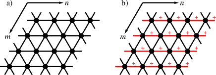
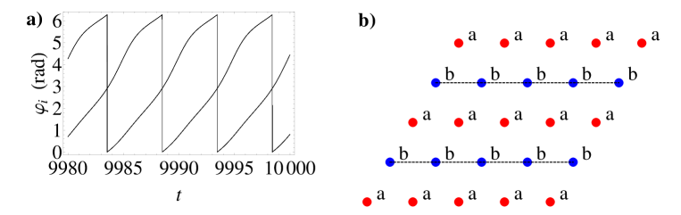
Here denote the natural “frequencies” of the rotators, and parameterize, respectively, the level of excitability and the coupling strength. Further, denotes the number of neighbors to which the -th unit is connected, and is the adjacency matrix with , if and units and are connected, otherwise . The terms and denote multiplicative and additive white noise, respectively, with , , likewise , where and are measures for the multiplicative and additive noise intensities, respectively. Throughout the paper we set : for a set of identical elements the synchronized solution always exists on arbitrary plane lattices, in contrast to two-dimensional lattices of oscillators with distributed frequencies Hong_Park . We choose to represent a hexagonal lattice of the size with periodic boundary conditions, unless otherwise stated, as shown in Fig. 1 (a), so that each unit has the same number of nearest neighbors: .
Most former studies have been performed for positive coupling , while we are mainly interested in repulsive coupling and choose . The reason is that negative in combination with the hexagonal coupling pattern turns all bonds into frustrated. Consider any elementary triangle formed by units . Negative coupling ensures that unit prefers to be antiphase to and prefers to be antiphase to . As a result, would be in phase to , which is in conflict with the repelling direct link between them. So whatever phase the unit assumes, the bond either between and or between and is frustrated.
In order to compare our results with couplings that are disordered with respect to their sign, but do not lead to any frustrated bonds, we show also the case of positive couplings for the bonds along the horizontal directions in Fig. 1 (b), while all other bonds are repulsive.
III Multistability for repulsive coupling
Kuramoto oscillators. Consider eq. (1) with both sources of noise set to zero. Let us first discuss the phase space structure for : a set of Kuramoto oscillators coupled on a hexagonal -lattice. By going into the comoving frame via and rescaling the time via the normalized coupling strength (for the given number of nearest neighbors), we arrive at
| (2) |
While for positive this system has a single stable fixed point in which all phases are the same (this corresponds to synchronous oscillations with frequency in the lab frame), we see hints on the expected multistability for the negative coupling for a subset of solutions. These are plane-wave solutions, characterized by fronts of constant phases along parallel lines on the hexagonal lattice such that no nearest neighbors share the same phase. Their spatial distribution is characterized by
| (3) |
for coordinates and , where allowed values for the wave vector are restricted to integers by the periodic boundary conditions. In patterns of this kind the coupling term identically vanishes. For this set we show in the Appendix A.1 that for a sufficiently large extension of the lattice and an even number of the linear extension , there are always two sets of wave vectors and such that the plane waves correspond to different solutions. These solutions do not merely differ by a rotation of the linear front, but by the very number of oscillators sharing the same phase (below we denote such sets of oscillators as “clusters”).
Plane-wave solutions, which obviously reflect the lattice symmetry in their fronts of constant phases, are not the only stable solutions on a hexagonal lattice, as we shall discuss in more detail below.
Active rotators. In the following, without restriction of generality, we assume to be non-negative. For , by rescaling the time unit we set and follow the solutions in the parameter space of and . For and positive , active rotators have a stable fixed point, , , in which all elements are synchronized with the same phase. This fixed point is stable for sufficiently small negative as well; when is decreased, it loses stability via the degenerate pitchfork bifurcation at , where is the minimal (most negative) eigenvalue of the adjacency matrix . The corresponding derivation is provided in Appendix A.2. For the hexagonal lattice the minimal eigenvalue is always degenerate; its multiplicity depends on the periods and : for and == it equals 2; for = it equals 6 with the exception of the case ==4 when the multiplicity of the minimal eigenvalue is 9. Accordingly, the dynamics on the corresponding central manifold is not quite trivial. Leaving the complete description for the forthcoming publication, here we note only that, in spite of the high multiplicity, the gradient character of the dynamics forbids the complexification of eigenvalues, therefore no Hopf bifurcations can occur.
For sufficiently negative , when, at , every individual unit is in the limit-cycle state, there are no stable fixed points. Since we are primarily interested in the order-by-disorder effect, we do not further zoom into the bifurcation region, but choose sufficiently negative as to be well inside the parameter domain with time-dependent dynamics. This domain is characterized by coexisting states with different synchronization patterns which perform periodic or quasiperiodic oscillations. Even for small lattice sizes the number of coexisting attractors can be quite large, and below we briefly describe just two typical patterns.
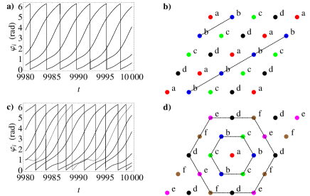
Similarly as for Kuramoto oscillators, one form of stable solutions are plane-wave patterns. They are characterized by fronts of identical phases which are parallel to each other and extend along straight lines of the hexagonal lattice as shown in Fig. 2 (b), connecting sites which are not nearest neighbors in accordance with the repulsive couplings. A special case of plane wave solutions are splay-like states for which the instantaneous values of phases characterizing different clusters are separated on the unit circle by equal intervals.
Another type of solution appears as a spherical wave on a hexagonal lattice. For example, it is found as a 6-cluster solution on a lattice with integer . At a first glance, the phase assignments on the -lattice, displayed in Fig. 2 (d), may look irregular; there the characters label different clusters. However, what we see is a sector of a “discretized” spherical wave on the hexagonal lattice, with an isolated oscillator in its center, surrounded by two clusters of three oscillators, in alternating order , along the first polygon ring of nearest neighbors. In the second ring of next-nearest-neighbors of the center, three clusters of three oscillators are arranged like . Phase differences within a ring and between different rings do not stay constant, but oscillate regularly. Placing on a -lattice the center of the wave into any of the 16 sites and performing any number of 60∘ rotations, we obtain 96 replicas of this configuration.
The existence of the described wave assumes compatibility with the lattice size and the boundary conditions; its stability depends on the strength of repulsive coupling.
Characterization of states. In view of our goal to analyze the order-by-disorder effect, it is sufficient to distinguish the states according to their cluster partitions: we denote the states as , being the overall number of clusters. We say that several oscillators belong to the same cluster if they share the same phase within numerical accuracy. This accuracy will be lowered and adapted in the presence of noise. Of course, this characterization is not unique: several different states can have (and as we will see below they do have indeed) the same partition into clusters. By different we mean dynamical distinctions: two states which cannot be transformed into each other by a combination of symmetry transformations of the lattice (translations, rotations, reflections); for periodic solutions, it suffices to have non-coinciding values of the period.
IV Order-by-disorder for active rotators
Quasi-stationary states. In the following we consider active rotators coupled with frustration on hexagonal lattices under the action of noise. Without noise, the stationary -states, characterized by their cluster partitions, correspond to frequency - synchronized oscillators, with phase-locked motion in case of Kuramoto oscillators, (that is time-constant phase differences between different clusters,) and oscillating phase differences between different clusters in case of active rotators.
In contrast, under the action of weak and moderate noise, the system exhibits behavior which we would call quasi-stationary. In fact, this is noisy dynamics on a landscape with many traps: the trajectory moves from one -state to another, spends there a noticeable amount of time, departs to the next one, and this ad infinitum. For strong noise the short intervals of stay can hardly be resolved and the motion turns into a random walk across the rough energy landscape.
We represent our results in terms of time evolutions of individual oscillator phases , a presentation which is limited by the spatial resolution for larger systems. The widespread characterization in terms of the Kuramoto order parameters has been designed for the case of uniformly rotating oscillators, and works especially well in the splay situation, when the phase clusters are more or less uniformly placed on the circle. There for the state the values of with (nearly) vanish, whereas the value of is close to 1. Since in our computations the values of phases in the clusters are typically not equally spread, the lower parameters are usually not small and can hardly serve as simple indicators. In case of active rotators the set of order parameters is even less appropriate: phase space of an active rotator involves segments of relatively fast and relatively slow evolution. Since major portions of time are spent on slow segments, the parameter would be close to 1 (and, hence, indicate synchrony) even in the case when the coupling is completely absent. It may also happen that the average over one time period of some takes a larger value for a state with less coinciding phases. Examples will be discussed below.
Our basic example is the lattice of size at =0.7, =1 and sufficiently strong negative coupling =–2. In the absence of noise, this lattice is especially multistable. Starting from different initial conditions (a sequence of randomly generated 2 sets) we were able to resolve here 75 stable periodic orbits of the type which have different values of the period and, hence, are dynamically different. Each of these orbits has a multitude of symmetric replicas. Besides, we detected two dynamically different spherical waves of the type : one of them corresponds to a limit cycle, and another one – to a quasiperiodic state. Finally, one periodic solution and several quasiperiodic states belong to the type : all instantaneous values of individual phases are different. The reason why we call the latter type a clustered pattern although each cluster consists of a single oscillator, is the fact that in this state the phases are still correlated: phase differences between the sixteen oscillators oscillate periodically or quasiperiodically. This regular character of oscillations persists at weak noise. In contrast, in the most disordered state that is observed for strong noise, the evolution of individual phases seems fully uncorrelated.
For detection of periodic and quasiperiodic states we used the numerically obtained Poincaré mapping on the hypersurface =const. Limit cycles turn into attracting fixed points of the mapping, whereas the quasiperiodic states (two-dimensional tori) are identified as smooth curves on the secant surface.
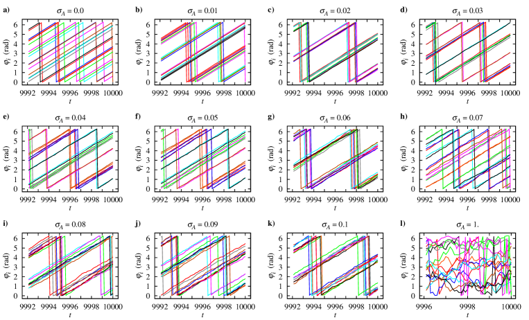
Now we turn on additive noise and monotonically increase its intensity. The results are shown in Fig. 3.
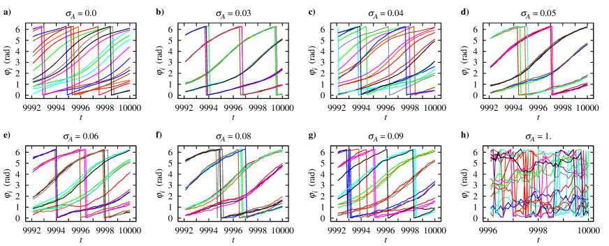
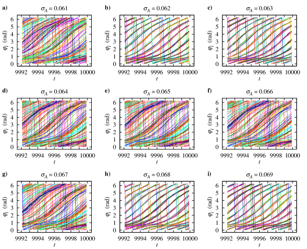
We plot the phases of all oscillators in the interval as functions of time. While the noise intensity is varied from to , all other parameters are kept fixed: , , . In the presence of noise, exact coincidence of phases is washed out, but the tendency to form easily recognizable groups persists, therefore we soften the definition: we say that oscillators belong to one cluster if their phases agree within for and within for , so that the accuracy has to be adapted to the noise intensity. If we characterize the solutions by the cluster partitions in terms of , and mark all disordered states by the symbol , we read off the following sequence from Fig. 3: (each oscillator is isolated) for ; (four clusters with four oscillators in each), for , , and later again for ; solutions consisting of one isolated oscillator, two clusters with three oscillators each and three clusters with three oscillators each around the center of the spherical wave, for , (, not displayed), (and , not displayed). The states as seen for and correspond to patterns, but for stronger noise the system stays in a more ordered realization of this pattern, which may give a hint on a deeper valley of the attractor in which the synchronization is less sensitive to the noise. For even stronger noise like the solutions get fully disordered: all phases are non-synchronized and uncorrelated. In terms of our notion of order, a 4-cluster solution is more ordered than a 6-cluster solution which is more ordered than a 16-cluster solution.
Generic features. For all realizations, displayed in Fig. 3, we varied only the intensity of additive noise, starting from the same randomly chosen initial condition, and choosing the same seed for the random number generator. The question therefore arises of how representative are these plots. Individual plots like those of Fig. 3 do depend on the boundary conditions (whether periodic or not), initial conditions (random or not), the realization of noise (additive, multiplicative, weak, intermediate, and the very realization), moreover on the time instant at which the snapshots are taken, and the lattice size. What is independent of the concrete choice of all these conditions is the observed non-monotonically varying degree of order when the noise intensity is monotonically increased. This feature should be observed as long as the boundary and initial conditions allow for many coexisting attractors in the system without noise, as we shall explain in the following.
We formed an ensemble of hundred randomly chosen initial conditions, and for each of them we repeated the simulation with ten different realizations of noise of the same intensity. Let us call the sequence , , , , , , , , , , , that is observed in Fig. 3 a “pattern”. If we view as “qualitatively the same pattern” those sequences which differ by permutations of the sequence or a different number of 6-cluster and 4-cluster solutions, then out of the hundred initial conditions led to qualitatively the same pattern as in Fig. 3. The remaining of initial conditions lead to sequences like with homogeneous behavior for a larger intermediate range of noise, in case of which the non-monotonic behavior is less pronounced. From the different realizations of noise for otherwise unchanged parameters about have led to qualitatively the same patterns, the actual numbers vary between one and six out of ten. We conclude that the observation of a sequence with a pattern as displayed in Fig. 3 is not a rare event in the stochastic dynamics of the ensemble.
It should be noticed that the patterns of Fig. 3 correspond to a short time window after time units from the start of integration and are not meant as final states. The sequence of order may differ for other, earlier and also (arbitrarily) later time windows, as we explain below. In particular, on sufficiently long time segments the solution of panel b) will repeatedly transform to and solution and back.
Similar, but visually more pronounced differences between more and less ordered and disordered states are recovered on a -lattice. Ordered states with ten clusters of ten oscillators each are seen for the intermediate noise intensities and , while we see hundred different phases, synchronized for zero or small noise values and fully disordered for large noise values, for the plots see (Fig. 4).
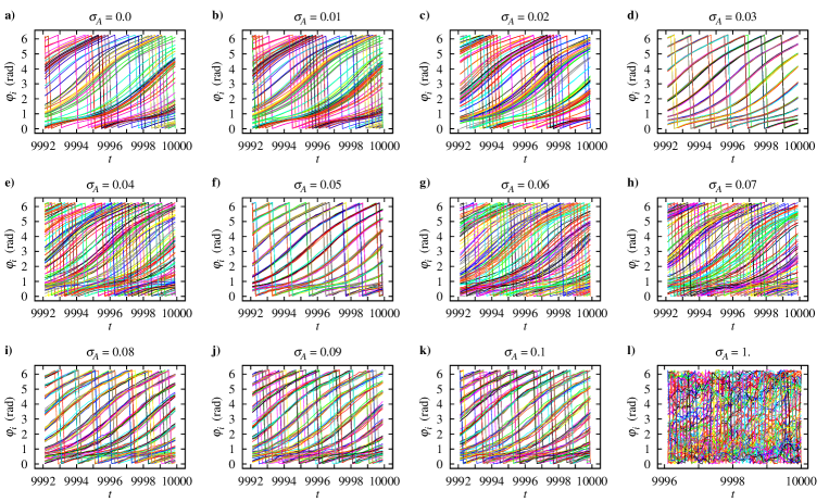
Remarkably, if we here further zoom into the noise intervals, for example into between the disordered patterns of hundred different phases at and (Fig. 5), we see a sequence like , for equidistant values of between to , where stands for hundred different phases and (order) for ten different phases organized in ten clusters.
At this point one may be tempted to continue the zooms to find out, down to which resolution of the noise intensity the characteristic order of the solutions within the same time interval (here ) persists. A variation of the noise in steps of for intervals within showed the same type of ordered solutions.
Again, all runs for different noise intensities started from the very same randomly chosen initial configuration of oscillator phases. Also here a slight change in the initial conditions may lead to different patterns as a function of the same increasing noise intensity. We observed similar pronounced non-monotonic behavior for about ten out of hundred different randomly chosen initial conditions.
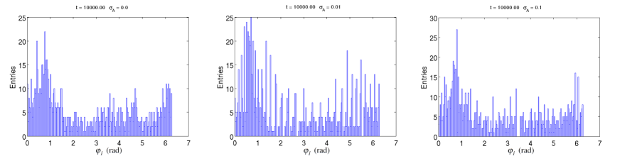
We have also identified order-by-disorder in larger systems like -lattices. Here we used histograms of the distribution of phases over the unit circle, which result from a collection of phase values at a fixed time instant (here time units from the start of integration.) For an intermediate value of the noise intensity (), the histogram has a more pronounced peak structure than for vanishing noise or for a strength of , see Fig. 6. For such systems we expect a multitude of attractors that is hard to resolve in its variety.
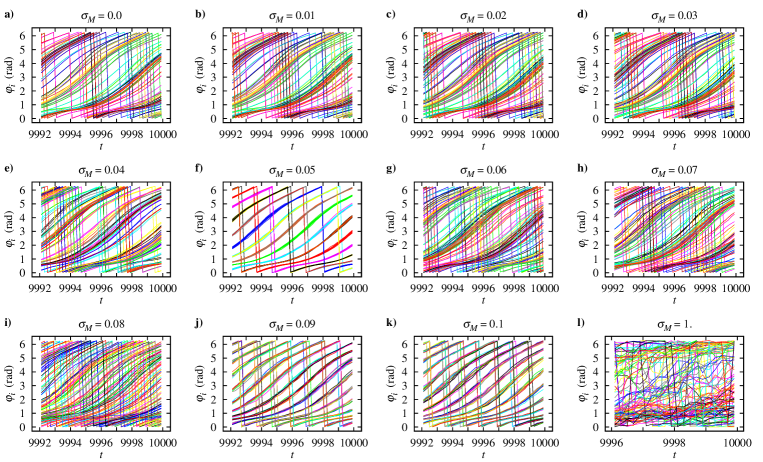
Order-by-disorder for multiplicative noise. Similar sequences of alternating synchronization patterns as in Fig. 3 are obtained, when the additive noise is replaced by multiplicative noise and is varied between and , with other parameters fixed at the same values. Here we again observe the effect of order-by-disorder for roughly of the different initial conditions; an example is shown for active rotators in Fig. 7.
Order-by-disorder for non-periodic boundary conditions. According to our numerical data, the discussed effect seems to be unrelated to the kind of boundary conditions on the lattice. As shown in Fig. 8, the tendency to formation of long-living clusters at small and moderate values of noise intensity persists for the lattice with free boundaries as well.
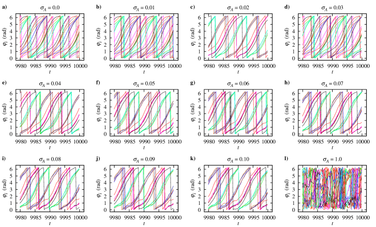
Order-by-disorder for Kuramoto oscillators. Kuramoto oscillators on the hexagonal lattice display similar sequences of states as in Fig. 3, confirming that the phenomenon is not caused by the excitability of the active rotators, but by the structure of the underlying potential landscape, which itself depends on the lattice topology and the sign-assignments of couplings. In Table 1 we illustrate why an alternative representation in terms of higher Kuramoto order parameters (here , , , and ) fails to reflect the order of states in full detail.
| panel | |||||
|---|---|---|---|---|---|
| 0.00 | a | 0.001 | 0.102 | 0.060 | 0.149 |
| 0.01 | b | 0.002 | 0.279 | 0.300 | 0.339 |
| 0.02 | c | 0.003 | 0.868 | 0.514 | 0.104 |
| 0.03 | d | 0.005 | 0.489 | 0.803 | 0.414 |
| 0.04 | e | 0.006 | 0.420 | 0.503 | 0.366 |
| 0.05 | f | 0.007 | 0.372 | 0.334 | 0.393 |
| 0.06 | g | 0.009 | 0.838 | 0.461 | 0.235 |
| 0.07 | h | 0.009 | 0.280 | 0.302 | 0.258 |
| 0.08 | i | 0.011 | 0.767 | 0.303 | 0.227 |
| 0.09 | j | 0.012 | 0.644 | 0.308 | 0.417 |
| 0.10 | k | 0.013 | 0.787 | 0.346 | 0.224 |
| 1.00 | l | 0.122 | 0.256 | 0.223 | 0.222 |
For example, in the noisy disordered state () they show larger values than for the initial state of vanishing noise intensity in panel (a) of Fig. 9. While otherwise adequately reflects the change in the order as observed in Fig. 9, fails for , where the order is less than for in contrast to what the order parameter suggests.
V Hierarchies in the potential barriers
We interpret the occurrence of more ordered and less ordered cluster partitions for monotonically increasing noise strength as an indication of a hierarchy in the potential barriers. In our system the role of a potential is played by the integral over of the equations (1), in terms of which the equations obey a gradient dynamics, , with given by
| (4) |
The first term in (4) is linear with respect to the phases and is responsible for the unbounded average drift whose slope is the same for all patterns. Two last terms, taken together, form the oscillatory part of the potential, . We evaluate for the 4-cluster solution, the 6-cluster solution, and the 16-cluster solution. The mean values over one period are , , and , respectively: the higher the order, the lower the corresponding potential. However, we possess no detailed knowledge about the landscape in between, in particular about the height of the ridges. Sensitive response to different noise intensities indicates that the landscape is quite rough, owing to the implemented high degree of frustration. Numerical evidence suggests that for a sizeable portion of initial conditions, deterministic paths to their eventual attractors pass close to one or several ridges, which makes them sensitive to the action of noise and introduces uncertainty in the destination.
In general, on the very large timescale, the time evolution of under the action of noise is a walk over the entire landscape. However, for the small and moderate noise intensities the residence times in vicinities of the deep minima or rifts are quite large (of the order of several hundred or thousand time units), whereas the shallow valleys are traversed relatively fast. Below we restrict ourselves to the moderately long epochs of evolution; hence, for shortness, these intermediate asymptotics near which the system spends long intervals of time, are referred to as “attractors”. It is these states that are displayed in Fig. 3. Furthermore, as indicated before, it is not the number of different patterns, characterized as , or , which defines the number of different attractors, since characterizations in terms of a pattern do not uniquely characterize a state due to the high degeneracy in assigning a pattern to the grid. Therefore, what we call “new attractors” below may share the same pattern as encountered before.
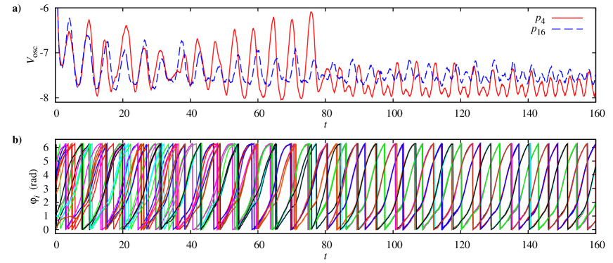
Consider an ensemble of stochastic trajectories which start from the same initial location in the high-dimensional landscape, that is, the ensemble is formed by different realizations of noise. Without noise, the gradient dynamics drives the phases along the gradient of the potential until the first local minimum or rift is met, where the system gets stuck, be it in a fixed point or in a limit cycle. Under sufficiently weak noise, the bulk of the trajectories of the ensemble remains close to the deterministic orbit and ends up at the same attracting set. Under somewhat stronger noise, the ensemble splits: part of the trajectories crosses the nearby ridge(s) and goes to different attractor(s), in contrast to the rest which follows the deterministic trajectory. This is what we have seen to occur in ten realizations. Fig. 10 (a) displays the temporal evolution of the oscillatory part of the potential for two trajectories which start from the same initial position under the same parameter values and correspond to two different realizations of additive noise at . The dashed line shows the trajectory which largely follows the deterministic solution and ends up at a pattern (the attracting state for these initial conditions in the absence of noise). The trajectory which is shown by the solid line, initially tracks the deterministic solution as well; however, after a certain time and a short epoch of strong oscillations, it appears to cross the ridge and land upon the deeper lying attractor of a solution. A closer look at the individual phases (Fig. 10 (b)) shows that transitional oscillations are close to the three-clustered state: apparently this is the unstable periodic solution, located on the ridge which separates the basins of and . The trajectory approaches this state along its stable manifold, spends some time (roughly the interval ) in its neighborhood, displaying larger amplitudes of , and leaves it along the unstable manifold. Very similar type of crossover behavior was found for and for different noise realizations, also leading to or patterns in the end.
Starting with yet a higher noise level, the overwhelming majority of trajectories cannot resolve the former basin of attraction any longer, as its shape gets buried under the noisy background; instead, the stronger noise enables the trajectories to explore the phase space in more remote regions from the starting point. It then depends on the depth of the valley whether the new attractor is able to keep the trajectory in its vicinity for a while and let the system settle inside the rift. Were the basin as shallow as the former one, the structure of the rift could not be recognized, and the transient passage of such a basin would not be identified as long-living metastable state in our simulations.
Now, as a matter of fact, our system finds repeatedly new attractors when the noise is increased. This may be either due to the presence of several ridges already in the vicinity of the starting point; it is then a random event which attractor is chosen under a new realization of noise, once its depth is sufficiently large. Or the new attractors are discovered when the noise drives the system a longer path through phase space, as long as an attractor in a more remote deep valley stops the walk for a transient time. Wherever the new attractors are located, with increasing noise they have to be increasingly deep to become observable. Naturally, trajectories visiting basins of attractions between the higher ridges will be less localized for stronger noise. This feature explains the need for adapting the size of the tolerance interval within which two phases are identified, see Fig. 3 (d) and (f).
For sufficiently high noise intensities, the whole potential structure is buried under the noise, and the phase trajectory performs a random walk, now driven by an effectively random potential, without correlations between individual phases, as it was seen in Fig. 3 (h). It should be noticed that Fig. 10(b) shows only the first 160 time units of the quasi-stationary state to illustrate the dispersion of the trajectories after about time units. The state remains time-dependent afterwards, as the system keeps jumping from one attractor to another in the presence of noise. The histogram of escape times from one type of ordered state to another (say from any of the to any of the -states) shows a multi-peak structure. More details will be presented in a forthcoming paper.
Analogy to stochastic resonance
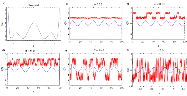
As an argument in favor of our conjecture of a hierarchical landscape with potential barriers of various depths, we demonstrate analogous behavior for stochastic resonance. To this aim we choose a one-dimensional potential with only two levels of barriers: , as shown in Fig. 11 (a). Unlike most studies of stochastic resonance, we are interested not in temporal (resonance-like) aspects of the dynamics, but in the localization of solutions in different basins.
Consider the motion of a particle, described by the stochastic differential equation
| (5) |
where is Gaussian white noise with intensity : , . An external subthreshold periodic perturbation does not allow the particle to leave any of the four local minima in the absence of noise, but combined with noise it triggers the switching between different minima. In Fig. 11 (b)-(f) the response of the system to increasing noise intensity is shown. For low intensity (), we observe very small random oscillations about one of the local minima, here about (Fig. 11 (b), red line). Regular oscillations in Figs. 11 (b)-(f) show the periodic external force (blue lines). For an optimal noise strength (), the particle is enabled to cross the lower barrier, so it jumps in resonance with the external frequency between and (or, depending on the initial conditions, and ) (Fig. 11 (c)). For an intermediate larger noise intensity the motion between and is irregular (Fig. 11 (d)). For crossing the second barrier, there is the second “optimal” noise strength for which the particle jumps in resonance with the external frequency between locations in the interval and (Fig. 11 (e)). For even larger noise the particle does no longer see the underlying shape of the potential, but moves irregularly between the outer walls (Fig. 11 (f)). We see that under higher noise intensity the localization occurs on levels separated by higher barriers, and the particle is less localized in the vicinity of the minima. This reduced localization is akin to our need for adapting the tolerance interval when two rotator phases are identified within an uncertainty of .
VI Disorder in the coupling signs, but no frustration
Without frustration, but with disorder in the coupling signs according to the choice as in Fig. 1 (b), we have neither seen a signature for multistability, nor for the order-by-disorder phenomenon in oscillators. On a -lattice with otherwise the same choice of parameters we started from randomly chosen initial conditions, and from for a -lattice. The only stationary state we have found were 2-cluster solutions with oscillators in cluster aligned along a horizontal line and alternating with oscillators in cluster along the succeeding horizontal line, where the phase difference between clusters and fluctuates about (see Fig. 12).
VII Summary and conclusions
It is well known that the role of noise in nonlinear systems can be quite versatile lutz : in particular, it can increase the order in a disordered system. Here we made use of a similar mechanism that is known from spin systems with an analogous role played by the temperature there and noise here: we have chosen the topology and the couplings in a way as to induce frustrated bonds. Frustration leads to a considerable increase in the number of attracting states. Since the units are oscillatory, coexisting states are no longer restricted to fixed points as in spin systems, but can also be different patterns of phase-locked motion. The energy landscape is not necessarily degenerate, but the system is multistable. Similarly to spin systems, here the noise can temporarily increase the order of states, a fact that we called order-by-disorder. Surprisingly, however, as a function of monotonically increasing noise intensity we observe not only a maximum of order at some optimal noise intensity, as one may have expected from analogous results on stochastic resonance stoch , coherence resonance coh , or system size resonance sys . Instead we record an alternating sequence of higher and lower order among the oscillator phases, so that the variation of the noise intensity appears to “scan” a rough potential landscape with a hierarchy of potential barriers. To turn it into a practical device for scanning similar kinds of potential, the high sensitivity to the initial conditions should be reduced by adding appropriate control terms to the dynamics. Interestingly, the quasi-stationary state in the presence of noise shows a variety of time scales, realized in the escape times from one to another “attractor” (metastable state), which we shall further explore in a forthcoming paper.
Acknowledgements.
Two of us (F.I. and D.L.) would like to thank the Deutsche Forschungsgemeinschaft (DFG, contract ME-1332/19-1) for financial support. M.A.Z. was supported by the DFG Research Center MATHEON (Project D21).References
- (1) J. Villain, R. Bidaux, J.P. Carton, R. Conte, J. Phys. (France) 41, 1263 (1980)
- (2) D. Bergman, J. Alicea, E. Gull, S. Trebst, L. Balents, Nature Physics 3, 487 (2007)
- (3) R. Barnett, S. Powell, T. Graß, M. Lewenstein, S. Das Sharma, Phys. Rev. A 85, 023615 (2012)
- (4) J.N. Reimers, A.J. Berlinsky, Phys. Rev. B 48, 9539 (1993)
- (5) A. Chubukov, Phys. Rev. Lett. 69, 832 (1992)
- (6) R. Moessner, J.T. Chalker, Phys. Rev. B 58, 12049 (1998)
- (7) C.L. Henley, Phys. Rev. Lett. 62, 2056 (1989)
- (8) A.M. Turner, R. Barnett, E. Demler, A. Vishwanath, Phys. Rev. Lett. 98, 190404 (2007)
- (9) H. Sakaguchi, S. Shinomoto, Y. Kuramoto, Prog. Theor. Phys. 79, 600 (1988)
- (10) C.J. Tessone, D.H. Zanette, R. Toral, Eur. Phys. J. B 62, 319 (2008)
- (11) D.H. Zanette, Europhys. Lett. 72, 190 (2005)
- (12) H. Hong, S.H. Strogatz, Phys. Rev. E 84, 046202 (2011)
- (13) H. Daido, Phys. Rev. Lett. 68, 1073 (1992)
- (14) P. Kaluza, H. Meyer-Ortmanns, Chaos 20, 043111 (2010)
- (15) H. Hong, H. Park, M.Y. Choi, Phys. Rev. E 72, 036217 (2005)
- (16) B. Lindner, J. Garcia Ojalvo, A. Neiman, L. Schimansky-Geier, Physics Reports 392, 321 (2004)
- (17) L. Gammaitoni, P. Hänggi, P. Jung, F. Marchesoni, Rev. Mod. Phys. 70, 223 (1998)
- (18) A.S. Pikovsky, J. Kurths, Phys.Rev.Lett. 78, 775 (1997)
- (19) R. Toral, C.R. Mirasso, J.D. Gunton, Europhys. Lett. 61, 162 (2003)
Appendix A
A.1 Multistability for plane waves in Kuramoto oscillators
In the corotating reference frame the existence of steady states for Kuramoto oscillators is independent on the coupling strength, while their stability depends on the coupling sign. Here we formulate sufficient stability conditions for a certain class of fixed points, and for the coexistence of multi-stable solutions.

On the hexagonal lattice, the equation of motion for each oscillator includes 6 terms. We restrict ourselves to the plane waves with the pattern (3): ; there, the terms cancel pairwise, hence every solution of this form is an equilibrium point. Let the coupling strength be negative.
In the symmetric Jacobian matrix for an equilibrium of this kind, each row includes 7 non-zero elements. The non-zero off-diagonal elements are, respectively, two elements , two elements and two elements . The diagonal elements equal . Since the sum in every row vanishes, the Jacobian always possesses the zero eigenvalue which corresponds to the translational invariance of the equations of motion (2).
If all off-diagonal elements are negative, that is,
| (6) |
then the Jacobian matrix has no positive eigenvalues. Indeed, by splitting the Jacobian into the diagonal and the off-diagonal matrices we observe, as a consequence of the Frobenius-Perron theorem, that none of the eigenvalues of the non-diagonal part exceeds in the absolute value the (negative) diagonal element. This implies stability for the considered plane wave solution.
Note that this condition is not necessary: it does not include e.g. the patterns of spherical waves, which are numerically observed as stable solutions as well.
Next we use the same framework to demonstrate coexistence on sufficiently large lattices of plane waves (3) which differ by their number of clusters. For the case of the square lattice with , condition (6) is reduced to . For this interval contains at least two integers. Taking an even 18 and two consecutive integers and +1 from the stability interval, we observe that the first one corresponds to the pattern with clusters, where is the greatest common divisor of and , whereas the second one corresponds to clusters. Since two consecutive integers have no nontrivial common divisors, whereas a divisor 2 is shared between and either or +1, the numbers of clusters in two stable steady patterns cannot coincide.
A.2 Stability of the “synchronous” fixed point for active rotators
Here we discuss the synchronous steady solution for Eq.(1). We set, without restrictions of generality, =1 and work in the parameter space of and .
We start from the non-coupled case . For there are fixed points, defined by , with and . For linearizations of (1) at these points, the number of positive eigenvalues of the respective Jacobian equals the number of components . Accordingly, out of steady states –2 are saddles, one is stable, and one is unstable. For the stable equilibrium the values of each coordinate equals .
Now we switch on the coupling . Notably, the location of this equilibrium in the phase space is independent of . For the corresponding Jacobian we obtain
| (7) |
so that
| (8) |
where , as above, is the number of nearest neighbors on the lattice. The eigenvalues of are
| (9) |
where are the eigenvalues of the adjacency matrix. For =0, all eigenvalues of are negative. For , the first eigenvalue that becomes positive corresponds to the minimal eigenvalue of , , provided . The transition takes place at
| (10) |
here the stable fixed point loses stability and becomes a saddle. Notably, for a hexagonal lattice (=6) the minimal eigenvalue is always degenerate.
Our numerical observations on the hexagonal lattices suggest that the synchronous equilibrium has a large basin of attraction for sufficiently small weak negative couplings: this attractor was the only one which we found for different randomly chosen initial conditions on various lattice sizes (, , and ) and , , . On the other hand, for values , multistable solutions were easily found by starting from different initial conditions, solutions with clusters of phase locked oscillators that performed limit cycles. Therefore one may wonder whether multistable fixed point solutions exist as well. Such coexisting fixed point solutions can be identified for the case of , starting from initial conditions, which are given by phase distributions that are known from Kuramoto oscillators for () and otherwise the same choice of parameters, but then turning on . Since we can absorb in the time scale (setting ), we checked the stability of these fixed point solutions under tuning to more negative values, keeping . Using the Newton Raphson method, we found coexisting fixed points for which differ in the cluster partition of coinciding phases. For the coexisting fixed-point solutions see Fig. 13.