The Lee-Wick Standard Model at Finite Temperature

Abstract

The Lee-Wick Standard Model at temperatures near the electroweak scale is considered, with the aim of studying the electroweak phase transition. While Lee-Wick theories possess states of negative norm, they are not pathological but instead are treated by imposing particular boundary conditions and using particular integration contours in the calculation of S-matrix elements. It is not immediately clear how to extend this prescription to formulate the theory at finite temperature; we explore two different pictures of finite-temperature LW theories, and calculate the thermodynamic variables and the (one-loop) thermal effective potential. We apply these results to study the Lee-Wick Standard Model and find that the electroweak phase transition is a continuous crossover, much like in the Standard Model. However, the high-temperature behavior is modified due to cancellations between thermal corrections arising from the negative- and positive-norm states.

I Introduction

The Lee-Wick Standard Model (LWSM) Grinstein:2007mp is an extension of the Standard Model (SM) that tames the Higgs mass hierarchy problem by modifying the dispersion relationships of the various SM fields in order to improve the UV behavior of the theory. This modification is accomplished by introducing a new mass scale $\Lambda_{\text{\sc lw}}$ and extending the Lagrangian by dimension-six operators of the forms $\delta\mathcal{L}=(\Box\phi)^{2}/\Lambda_{\text{\sc lw}}^{2}$ and $\delta\mathcal{L}=\bar{\Psi}i(\not{\partial})^{3}\Psi/\Lambda_{\text{\sc lw}}^{2}$ and $\delta\mathcal{L}={\rm Tr}\left[D^{\mu}F_{\mu\nu}D^{\alpha}F_{\alpha\beta}\right]g^{\nu\beta}/\Lambda_{\text{\sc lw}}^{2}$. As such, the propagators fall off more rapidly in the ultraviolet (UV) limit above the scale $\Lambda_{\text{\sc lw}}$, which softens the divergences in one-loop corrections to the Higgs self-energy from dangerous quadratic ones to harmless logarithmic ones. To eliminate the need for fine tuning, $\Lambda_{\text{\sc lw}}$ should be not much larger than the electroweak scale.

Since the LWSM augments the SM by new degrees of freedom at the electroweak (EW) scale that are coupled to the Higgs (and indeed, one can study a variant LWSM in which only these fields are significant Carone:2008bs ), it is natural to expect the new physics to affect the nature of the electroweak phase transition. This connection is further motivated by the relationship between UV quadratic divergences and the phenomenon of symmetry restoration Comelli:1996vm . That is, the same Feynman graphs that give rise to quadratic divergences in the Higgs self-energy also yield $O(T^{2})$ corrections to the effective mass at finite temperature, and thereby lift the tachyonic Higgs mass and induce symmetry restoration. In previous work, the free energy density and thermodynamic properties of the LWSM plasma have been calculated Fornal:2009xc , and the non-thermal effective potential has been derived Espinosa:2011js . The goal of this paper is to study the LWSM at finite temperature using the thermal effective potential in order to determine the nature of the electroweak phase transition and symmetry restoration.

The LWSM Lagrangian contains higher-order time derivatives of the various SM fields, which leads to roughly a doubling of the number of dynamical degrees of freedom. It is well-known that such higher-derivative (HD) theories generally suffer from a variety of pathologies (see, e.g., Hawking:1985gh ; Hawking:2001yt for a pedagogical discussion). At the classical level, Ostrogradsky’s theorem forces the Hamiltonian to be unbounded from below due to excitations of the new degrees of freedom. If one departs from the canonical quantization prescription in quantizing the theory, then the spectrum can be rendered bounded from below, but at the cost of introducing states of negative norm, i.e., ghosts. Lee and Wick developed a prescription for removing the ghosts and rendering the theory predictive by treating the system as a boundary-value problem and imposing boundary conditions at future infinity Lee:1969fy ; Lee:1970iw (see also Cutkosky:1969fq ). Subject to these boundary conditions, the system develops an acausal behavior on the timescale $\Lambda_{\text{\sc lw}}^{-1}$. For $\Lambda_{\text{\sc lw}}=O(\rm{TeV})$, the acausality is confined to microscopic scales, and thereby evades constraints from direct laboratory observation.

Due to the pathologies of HD theories, it is a priori unclear how to correctly and consistently formulate a calculation at finite temperature. To illustrate where the trouble arises, consider a classical HD theory. At finite temperature, a system approaches thermal equilibrium by redistributing energy between its many degrees of freedom so as to minimize its energy and maximize its entropy. However, for a system in which the Hamiltonian is unbounded, the entropy can always be increased without bound by lowering the energy of some degrees of freedom and raising the energy of others. This discussion illustrates why care must be taken in formulating the calculation at finite temperature.

Developing the correct formulation of Lee-Wick theories at finite temperature is one of the goals of this paper. Previous efforts to tackle this problem have taken different approaches: One group studied an ideal gas of negative-energy particles Bhattacharya:2011bb , whereas a second group studied the partition function of SM particles that are able to scatter through negative-norm narrow resonances Fornal:2009xc . Both groups concluded that the contribution from a LW field to the free energy is precisely the opposite of that from a SM field with identical mass and spin. However, a third group argued that the connection between symmetry restoration and UV behavior suggests that a relative minus sign should not appear Espinosa:2011js . In Sec. III we explore and extend the previous work by first addressing whether it is more realistic to treat the LW fields as an ideal gas or as resonances, and second by addressing the issue of the sign. On the second point, we introduce an index $\sigma=\pm 1$ in order to consider both sign choices simultaneously and thereby keep our analysis general. For the case $\sigma=+1$($-1$), the LW fields contribute to the free energy density with the same (opposite) sign as SM fields, and it is from this perspective that we proceed to study the LWSM at finite temperature. We find that the two cases lead to qualitatively different outcomes with regard to the temperature of the electroweak phase transition, as well as the sign of thermodynamic quantities in the ultra-relativistic limit.

This paper is organized as follows. For the reader who is unfamiliar with Lee-Wick theories, we provide a more detailed introduction to the subject in Sec. II. In Sec. III we formulate the thermodynamics of Lee-Wick theories and calculate the one-loop thermal effective potential for a toy model. In Sec. IV we evaluate the thermal effective potential for the LWSM and study the LWSM at finite temperature, determine the nature of the electroweak phase transition, and investigate the phenomenon of symmetry restoration. In Sec. V we summarize and conclude. Appendix A describes possible quantization conventions, and App. B gives details of the LWSM spectrum.

II Introduction to Lee-Wick Theories

The Lee-Wick Standard Model Grinstein:2007mp was developed by Grinstein, O’Connell, and Wise as an alternative approach to taming the gauge hierarchy problem of the Standard Model. In the case of the much better-explored example of low-scale supersymmetry (SUSY), each SM loop diagram is joined by one in which the loop particle is replaced by its opposite-statistics partner (but which carries the same gauge and Yukawa couplings), thus introducing a relative sign difference that induces the cancellation of the leading-order (quadratic) divergence. In the LWSM, each loop diagram is joined by one in which the loop particle is replaced by its opposite-norm partner, again inducing the desired cancellation.

The essence of the original Lee and Wick program Lee:1969fy ; Lee:1970iw is the promotion of Pauli-Villars regulators to the status of full dynamical fields with negative quantum-mechanical norm. Obviously, such unusual states introduce paradoxes of physical interpretation that must be addressed. At the classical level, such signs correspond to instabilities in the form of runaway states of ever-increasing negative energy, while at the quantum level a negative norm (which generates a Hilbert space of indefinite metric Pauli:1943xx ) produces a violation of unitarity. However, Lee and Wick showed that these runaway solutions can be eliminated from the theory by the imposition of future boundary conditions on Green’s functions, which has the price of introducing violations of causality. If the LW scale is sufficiently high, then the realm of acausal effects is relegated to an unobservably microscopic scale. Moreover, if the negative-norm states are required to be unstable (decaying into conventional particles), then they may be excluded from the set of asymptotic states of the theory, thus restoring unitarity. In order for the exclusion of on-shell negative-norm states to make sense in Feynman loop diagrams, Lee and Wick developed a variant of the Feynman integration contour for such cases, a program that was greatly expanded by Cutkosky et al. Cutkosky:1969fq (CLOP). While no problematic exceptions to this program are known, it remains unknown whether a nonperturbative formulation exists that preserves unitarity Boulware:1983vw .

In the same way that adding a Pauli-Villars regulator to a scalar propagator softens its high-momentum behavior from $~{}1/p^{2}$ to $~{}1/p^{4}$, the Lagrangian of a scalar theory containing a particle and its LW partner is promoted from one with a canonical $\partial^{2}$ kinetic energy term to a higher-derivative theory with a $\partial^{4}$ term. To be explicit, let $\hat{\phi}$ be a real scalar field appearing in the Lagrangian

$${\cal L}_{{\rm HD}}=-\frac{1}{2}\hat{\phi}\,\Box\,\hat{\phi}-\frac{1}{2\Lambda_{\text{\sc lw}}^{2}}\hat{\phi}\,\Box^{2}\hat{\phi}-\frac{1}{2}m^{2}\hat{\phi}^{2}+{\cal L}_{{\rm int}}(\hat{\phi})\,,$$ (1)

where the last term represents interactions. One may recast Eq. (1) in an equivalent form without the HD term by introducing an auxiliary field (AF) $\tilde{\phi}$:

$${\cal L}_{{\rm AF}}=-\frac{1}{2}\hat{\phi}\,\Box\,\hat{\phi}-\frac{1}{2}m^{2}\hat{\phi}^{2}-\tilde{\phi}\,\Box\,\hat{\phi}+\frac{1}{2}\Lambda_{\text{\sc lw}}^{2}\tilde{\phi}^{2}+{\cal L}_{{\rm int}}(\hat{\phi})\,.$$ (2)

The equation of motion for $\tilde{\phi}$,

$$\tilde{\phi}=\frac{1}{\Lambda_{\text{\sc lw}}^{2}}\Box\,\hat{\phi}\,,$$ (3)

is exact at the quantum level (meaning that the path integral over this degree of freedom can be performed exactly), and upon substitution into Eq. (2), reproduces Eq. (1). Further defining the field $\phi\equiv\hat{\phi}+\tilde{\phi}$ diagonalizes the kinetic energy terms:

$${\cal L}=-\frac{1}{2}\phi\,\Box\,\phi+\frac{1}{2}\tilde{\phi}\,\Box\,\tilde{\phi}-\frac{1}{2}m^{2}(\phi-\tilde{\phi})^{2}+\frac{1}{2}\Lambda_{\text{\sc lw}}^{2}\tilde{\phi}^{2}+{\cal L}_{{\rm int}}(\phi-\tilde{\phi})\,.$$ (4)

One diagonalizes the mixed mass terms without altering the kinetic terms by a symplectic transformation:

$$\left(\begin{array}[]{c}\phi\\ \tilde{\phi}\end{array}\right)=\left(\begin{array}[]{cc}\cosh\theta&\sinh\theta\\ \sinh\theta&\cosh\theta\end{array}\right)\left(\begin{array}[]{c}\phi_{0}\\ \tilde{\phi}_{0}\end{array}\right)\,,$$ (5)

with mass eigenstates being indicated by subscript $0$, and the transformation parameter $\theta$ satisfies

$$\tanh 2\theta=\frac{-2m^{2}}{\Lambda_{\text{\sc lw}}^{2}-2m^{2}}\,,$$ (6)

which admits real solutions provided $\Lambda_{\text{\sc lw}}^{2}>4m^{2}$. If this LW stability condition fails, then the kinetic and mass terms cannot be simultaneously diagonalized with real mass eigenvalues, and the Lagrangian Eq. (1) does not represent a Lee-Wick theory. The Lagrangian then assumes the form

$${\cal L}_{{\rm LW}}=-\frac{1}{2}\phi_{0}\,\Box\,\phi_{0}+\frac{1}{2}\tilde{\phi}_{0}\,\Box\,\tilde{\phi}_{0}-\frac{1}{2}m_{0}^{2}\phi_{0}^{2}+\frac{1}{2}M_{0}^{2}\tilde{\phi}_{0}^{2}+{\cal L}_{{\rm int}}[e^{-\theta}(\phi_{0}-\tilde{\phi}_{0})]\,,$$ (7)

for mass eigenvalues

$$m_{0}^{2},\,M_{0}^{2}\equiv\frac{\Lambda_{\text{\sc lw}}^{2}}{2}\left(1\mp\sqrt{1-\frac{4m^{2}}{\Lambda_{\text{\sc lw}}^{2}}}\right)\,,$$ (8)

and the factor of $e^{-\theta}$ can be absorbed into redefinitions of the couplings. The quadratic terms in Eq. (7) clearly manifest the promised opposite-norm $\phi_{0}$ and $\tilde{\phi}_{0}$ propagators (see App. A). This fact, combined with the fixed relationship between $\phi_{0}$ and $\tilde{\phi}_{0}$ couplings seen in ${\cal L}_{{\rm int}}$, leads to the cancellation of quadratic divergences, as shown explicitly in Ref. Grinstein:2007mp . While we have presented only the LW construction for a real scalar field, an analogous AF construction holds for all SM fields Grinstein:2007mp : complex scalars (with or without spontaneous symmetry breaking), Dirac fermions, and vector fields (including gauge fields).

We see that SM particles with LW partners can be represented by HD fields appearing in a restricted class of Lagrangians (so that the mass eigenvalues turn out real and positive) whose propagators fall off as $1/p^{4}$ and have two propagator poles, which represent one field of positive and one of negative norm. But nothing in principle requires the HD theory to truncate at just two extra derivatives. One can define a LW theory of a given $N$ as one in which the full propagator has $N$ poles, or equivalently, $2N$ extra derivatives in the Lagrangian. The SM would therefore be called an $N=1$ theory, the LWSM would be $N=2$, and as shown in Ref. Carone:2008iw , one can build $N\geq 3$ theories for all fields appearing the SM, including a proper AF construction. Furthermore, one finds that the additional field degrees of freedom alternate in norm: Each $N=3$ field, like its SM partner, has positive norm. Such a generalized LW theory is quite unlike SUSY and rather more resembles theories with Kaluza-Klein (KK) excitations, such as extra-dimension models.

Nevertheless, LW theories are unlike both SUSY and KK theories in important respects. Since no principle dictates how many LW partners a given SM field possesses nor what determines the LW scale, one can imagine a scenario in which some SM fields have 2 partners, some have 1, and some have none. In contrast, the closure of the SUSY algebra requires every field to have precisely one opposite-statistics partner, while KK theories have no predetermined limit on the number of modes available to the field. This generality of LW theories of course comes at a price. To name just a few issues: In fits to data or in making predictions, one must allow for the possibility that all field LW mass scales are distinct; the equivalent HD theory may only be an effective theory of an unknown UV completion (for our purposes, we assume only that the effective theory is good up to the 14 TeV reach of the Large Hadron Collider); and while grand unification is possible Grinstein:2008qq ; Carone:2009it , it is not as straightforward to arrange as in, say, the MSSM. Even so, LW theories are quite flexible and can be combined with other beyond-SM (BSM) ideas like SUSY Dias:2012fi ; Gama:2011ws .

The LWSM was subjected to tests of its phenomenological viability as a potential BSM theory already starting in Ref. Grinstein:2007mp , and subsequently compared to precision electroweak constraints in a variety of interesting ways Alvarez:2008za ; Underwood:2008cr ; Carone:2008bs ; Chivukula:2010nw ; Krauss:2007bz ; Carone:2009nu ; Alvarez:2011ah ; Figy:2011yu . The consensus view emerged that LW gauge bosons must have masses at least $~{}2$ TeV and the LW fermions at least several TeV, but the LW scalars can be substantially lighter. When $N=3$ partners are permitted, the allowed gauge boson partner masses must still be at least 2 TeV or higher, and the fermions may be as low as $1.5$ TeV, but viable scenarios in which the scalar partners lie in the several hundred GeV range emerge Lebed:2012ab .

III Thermodynamics of Lee-Wick Theories

In this section we address the question of how one should calculate the thermodynamic properties (e.g., entropy, energy density) of a LW theory. It is unclear to what extent the standard formulation of this calculation is applicable due to the presence of unphysical degrees of freedom, namely, the negative-norm LW particles. At zero temperature, one imposes boundary conditions to remove the LW particles from the set of asymptotic states and employs the LW/CLOP prescriptions to calculate elements of the unitary S matrix between states containing only SM particles. It is not obvious how to extend the boundary conditions and LW / CLOP prescriptions to a LW theory at finite temperature. Thus, two pictures emerge: Either

• The thermal system can access states containing explicit LW particles, or

• The system can only explore states from which these explicit LW particles are absent.

Both scenarios have been considered in the literature (Bhattacharya:2011bb and Fornal:2009xc , respectively). In fact, Ref. Bhattacharya:2011bb obtains the same result for the free energy as Ref. Fornal:2009xc . We argue, however, that the pictures are not equivalent, but instead that the second picture, in which LW particles only serve to modify the scattering of SM particles, is more realistic. In the next subsection we show that no self-consistent calculation using ideal gas LW particles appears to agree with the common result of Refs. Fornal:2009xc ; Bhattacharya:2011bb . Furthermore, Ref. Bhattacharya:2011bb uses a convention of negative-energy, positive-norm particles, while Ref. Fornal:2009xc uses negative-norm, positive-energy particles. While we adopt the second convention, the first one can be shown to be equivalent if properly implemented (see App. A).

III.1 Ideal Gas of LW Particles

In this section, we consider the first of the two pictures discussed above and calculate the thermodynamic properties of an ideal gas of LW particles. A LW theory contains both SM and LW particles, but in the absence of interactions, their ideal gas contributions can be evaluated separately. We define the partition function $Z$ by the requirement that the density matrix,

$$\hat{\rho}=\frac{1}{Z}{\rm exp}(-\beta\hat{H})\,,$$ (9)

is properly normalized (see below). With interactions turned off, the spectrum of the Hamiltonian $\hat{H}$ consists of the vacuum $\bigl{|}0\bigr{>}$, single-particle states $\bigl{|}\bf p\bigr{>}$, and multi-particle states $\bigl{|}{\bf p}_{1},{\bf p}_{2},\ldots,{\bf p}_{N}\bigr{>}$ with the appropriate symmetrization (anti-symmetrization) for bosons (fermions). For example,

$$\bigl{|}{\bf p}_{1}\,{\bf p}_{2}\bigr{>}=\frac{1}{\sqrt{2}}\left(\bigl{|}{\bf p}_{1}\bigr{>}\otimes\bigl{|}{\bf p}_{2}\bigr{>}+\eta_{S}\bigl{|}{\bf p}_{2}\bigr{>}\otimes\bigl{|}{\bf p}_{1}\bigr{>}\right)\,,$$ (10)

where $\eta_{S}=+1$ ($-1$) for bosons (fermions). The single-particle states satisfy $\hat{H}\bigl{|}{\bf p}\bigr{>}=E_{\bf p}\bigl{|}\bf p\bigr{>}$, where $E_{\bf p}=\sqrt{{\bf p}^{2}+m^{2}}$. These expressions use the quantization convention $\eta_{C}=+1$ of Eq. (84).

As discussed in Sec. II, states with an odd number of LW particles have a negative norm due to the wrong-sign commutation relation of the associated creation and annihilation operators. We use the index $\eta_{N}$ [see Eq. (84)] to keep track of this norm; for LW particles (SM particles) we have $\eta_{N}=-1$ ($+1$). For example,

$$\begin{array}[]{l}\bigl{<}0\bigl{|}0\bigr{>}=1\,,\\ \bigl{<}{\bf p}\bigl{|}{\bf q}\bigr{>}=\eta_{N}(2\pi)^{3}\,2E_{\bf p}\,\delta({\bf p}-{\bf q})\,,\\ \bigl{<}{\bf p}_{1}\,{\bf p}_{2}\bigl{|}{\bf q}_{1}\,{\bf q}_{2}\bigr{>}=(2\pi)^{6}\,2E_{{\bf p}_{1}}2E_{{\bf p}_{2}}\left[\delta({\bf p}_{1}-{\bf q}_{1})\,\delta({\bf p}_{2}-{\bf q}_{2})+\eta_{S}\,\delta({\bf p}_{1}-{\bf q}_{2})\,\delta({\bf p}_{2}-{\bf q}_{1})\right]\,,\end{array}$$ (14)

and so on. The negative norm implies that eigenvalues and expectation values differ by a sign. For instance,

$$\int\frac{d^{3}q}{(2\pi)^{3}}\frac{1}{2E_{\bf q}}\bigl{<}{\bf p}\bigr{|}\hat{H}\bigl{|}{\bf q}\bigr{>}=\eta_{N}E_{\bf p}\ \ ,$$ (15)

whereas the state $\bigl{|}\bf p\bigr{>}$ has eigenvalue $E_{\bf p}$. This distinction is particularly relevant for the calculation of the partition function. If we normalize the density matrix by requiring

$${\rm Tr}\,\hat{\rho}=1\ \ ,$$ (16)

then the partition function $Z={\rm Tr}\,e^{-\beta\hat{H}}$ is given by a sum of expectation values

$$Z=\bigl{<}0\bigr{|}e^{-\beta\hat{H}}\bigl{|}0\bigr{>}+\int\frac{d^{3}p}{(2\pi)^{3}}\frac{1}{2E_{\bf p}}\bigl{<}{\bf p}\bigr{|}e^{-\beta\hat{H}}\bigl{|}{\bf p}\bigr{>}+\int\frac{d^{3}p}{(2\pi)^{3}}\frac{1}{2E_{\bf p}}\int\frac{d^{3}q}{(2\pi)^{3}}\frac{1}{2E_{\bf q}}\bigl{<}{\bf p},{\bf q}\bigr{|}e^{-\beta\hat{H}}\bigl{|}{\bf p},{\bf q}\bigr{>}+\ldots\ .$$ (17)

In the case $\eta_{N}=-1$, the terms alternate in sign. Since the expectation values of $\hat{\rho}$ are not strictly positive, the possibility may arise that the sum of the eigenvalues of $\hat{\rho}$ becomes greater than unity, while $\hat{\rho}$ itself remains normalized in the sense of Eq. (16). It is not clear how to interpret such a density matrix. Alternatively, one can normalize the density matrix by imposing

$${\rm Tr}^{\prime}\hat{\rho}\equiv\sum_{\rm eigs}\hat{\rho}=1\,,$$ (18)

where Trace^′ is obtained by simply summing the eigenvalue spectrum of the operator. In this case, the norm of the states is irrelevant to the calculation, and its outcome is the standard ideal gas partition function. It is not a priori clear that this sum is finite; such an assertion is equivalent to assuming that the conditionally convergent series implied in Eqn. (16) is absolutely convergent. We do not dwell on the issue of which normalization condition is the “correct” one, and the following section makes this debate moot. However, we pedagogically consider both cases in order to illustrate the issues that arise when one treats the LW particles as an ideal gas.

We first calculate the partition function using the normalization condition Eq. (16). It is convenient to perform the standard transformations and work in a different basis (see, e.g., Kapusta:1989 ): One discretizes the momentum by imposing periodic boundary conditions, and writes the Hamiltonian $\hat{H}=\sum_{\bf p}\hat{h}_{\bf p}$ as a sum over the single-particle Hamiltonians $\hat{h}_{\bf p}=E_{\bf p}\hat{N}_{\bf p}$. The number operator $\hat{N}_{\bf p}$ has a spectrum

$$\hat{N}_{\bf p}\bigl{|}n_{\bf q}\bigr{>}=n_{\bf p}\,\delta_{{\bf p},{\bf q}}\bigl{|}n_{\bf p}\bigr{>}\,,$$ (19)

where $\bigl{|}n_{\bf p}\bigr{>}$ is the state containing $n_{\bf p}$ particles, each of momentum ${\bf p}$. In this basis, the partition function is given by

$$Z={\rm Tr}\,e^{-\beta\hat{H}}={\rm Tr}\,\prod_{\bf p}\,e^{-\beta E_{\bf p}\hat{N}_{\bf p}}=\prod_{\bf p}\sum_{n_{\bf p}=0}^{n_{\rm max}}\bigl{<}n_{\bf p}\bigr{|}e^{-\beta E_{\bf p}\hat{N}_{\bf p}}\bigl{|}n_{\bf p}\bigr{>}\,,$$ (20)

where $n_{\rm max}=\infty$ (1) for bosons (fermions). Noting that the norms are $\bigl{<}n_{\bf p}\bigl{|}n_{\bf p}\bigr{>}=(\eta_{N})^{n_{\bf p}}$, one finds

$$Z=\prod_{\bf p}\sum_{n_{\bf p}=0}^{n_{\rm max}}\left(\eta_{N}e^{-\beta E_{\bf p}}\right)^{n_{\bf p}}\,.$$ (21)

Taking the logarithm turns the product into a sum, which becomes an integral in the continuum limit. Dividing by the volume factor, one obtains the free energy density

$$\mathcal{F}=-(\beta V)^{-1}\ln Z=-\beta^{-1}\int\frac{d^{3}p}{(2\pi)^{3}}\ln\left[\sum_{n_{p}=0}^{n_{\rm max}}\left(\eta_{N}e^{-\beta E_{\bf p}}\right)^{n_{\bf p}}\right]\,.$$ (22)

The sum evaluated separately for bosons and fermions gives

$$\mathcal{F}=\begin{cases}\beta^{-1}\int\frac{d^{3}p}{(2\pi)^{3}}\ln\left(1-\eta_{N}\,e^{-\beta E_{\bf p}}\right)&{\rm bosons}\,,\\ -\beta^{-1}\int\frac{d^{3}p}{(2\pi)^{3}}\ln\left(1+\eta_{N}\,e^{-\beta E_{\bf p}}\right)&{\rm fermions}\,,\end{cases}$$ (23)

which can be combined as

$$\mathcal{F}=\eta_{S}\beta^{-1}\int\frac{d^{3}p}{(2\pi)^{3}}\ln\left(1-\eta_{S}\eta_{N}e^{-\beta E_{\bf p}}\right)\,,$$ (24)

where $\eta_{S}=+1$ for bosons and $\eta_{S}=-1$ for fermions. Had we imposed the alternative normalization condition Eq. (18), then the factor of $(\eta_{N})^{n_{\bf p}}$ would not have arisen:

$$\mathcal{F}^{\prime}=\eta_{S}\beta^{-1}\int\frac{d^{3}p}{(2\pi)^{3}}\ln\left(1-\eta_{S}e^{-\beta E_{\bf p}}\right)\,,$$ (25)

which is the standard free energy of an ideal gas.

	$\eta_{S}$	$\eta_{N}$	$\beta^{4}\mathcal{F}$	$\beta^{3}s$	$\beta^{4}\rho$
SM Boson	$+1$	$+1$	$+c_{0b}+c_{1b}\varepsilon$	$-4c_{0b}-2c_{1b}\varepsilon$	$-3c_{0b}-c_{1b}\varepsilon$
LW Boson (${\rm Tr}^{\prime}\hat{\rho}=1$)	$+1$	$-1$	$+c_{0b}+c_{1b}\varepsilon$	$-4c_{0b}-2c_{1b}\varepsilon$	$-3c_{0b}-c_{1b}\varepsilon$
LW Boson (${\rm Tr}\hat{\rho}=1$)	$+1$	$-1$	$-c_{0f}-c_{1f}\varepsilon$	$+4c_{0f}+2c_{1f}\varepsilon$	$+3c_{0f}+c_{1f}\varepsilon$
SM Fermion	$-1$	$+1$	$+c_{0f}+c_{1f}\varepsilon$	$-4c_{0f}-2c_{1f}\varepsilon$	$-3c_{0f}-c_{1f}\varepsilon$
LW Fermion (${\rm Tr}^{\prime}\hat{\rho}=1$)	$-1$	$-1$	$+c_{0f}+c_{1f}\varepsilon$	$-4c_{0f}-2c_{1f}\varepsilon$	$-3c_{0f}-c_{1f}\varepsilon$
LW Fermion (${\rm Tr}\hat{\rho}=1$)	$-1$	$-1$	$-c_{0b}-c_{1b}\varepsilon$	$+4c_{0b}+2c_{1b}\varepsilon$	$+3c_{0b}+c_{1b}\varepsilon$

Table 1: The thermodynamic properties of an ideal gas of SM or LW bosons or fermions in the high-temperature limit $\beta^{2}m^{2}\equiv\varepsilon\ll 1$. For the LW particles, the density matrix is normalized using either Eq. (16) or Eq. (18), as indicated. Higher-order terms in $\varepsilon$ are dropped. The coefficients are $c_{0b}\equiv-{\rm Li}_{4}(+1)/\pi^{2}=-\pi^{2}/90$, $c_{1b}\equiv{\rm Li}_{2}(+1)/4\pi^{2}\equiv 1/24$, $c_{0f}\equiv{\rm Li}_{4}(-1)/\pi^{2}=-7\pi^{2}/720=(7/8)c_{0b}$, and $c_{1f}\equiv-{\rm Li}_{2}(-1)/4\pi^{2}=1/48=(1/2)c_{1b}$.

These results are summarized in Table 1, where we also exhibit the entropy density $s=-\partial\mathcal{F}/\partial T$, and energy density $\rho=\mathcal{F}+Ts$. We have expanded in the high-temperature regime $\beta^{2}m^{2}\ll 1$ in order to facilitate comparison with more familiar expressions. When the density matrix is normalized by summing the spectrum, ${\rm Tr}^{\prime}\hat{\rho}=1$, one finds that the thermodynamics of a LW ideal gas is identical to that of a SM ideal gas of the same spin. This result is not surprising, since the negative-norm property never enters. On the other hand, when the density matrix is normalized by taking expectation values, ${\rm Tr}\,\hat{\rho}=1$, one finds that the LW boson has the same thermodynamics as a SM fermion with an overall sign flip, and vice versa. The negative entropy and energy densities are a distinctly counterintuitive result, since the LW 1-particle states have positive energy, and presumably should constitute an ideal gas with positive energy density. These results may be summarized schematically as

$${\rm Tr}^{\prime}\,\hat{\rho}=1: \mathcal{F}[\text{\small LW boson / fermion of mass $m$ }]=+\mathcal{F}[\text{\small SM boson / fermion of mass $m$ }]\,,$$ (26)

$${\rm Tr}\,\hat{\rho}=1: \mathcal{F}[\text{\small LW boson / fermion of mass $m$ }]=-\mathcal{F}[\text{\small SM fermion / boson of mass $m$ }]\,.$$ (27)

Both of these results differ from a previous calculation of the thermodynamics of LW ideal gas Bhattacharya:2011bb , which finds that the free energy, entropy, and energy densities of the LW gas are precisely the opposite of these quantities for the corresponding SM gas of the same spin, i.e.,

$$\begin{array}[]{l}\mathcal{F}[\text{\small LW boson / fermion of mass $m$ }]=-\mathcal{F}[\text{\small SM boson / fermion of mass $m$ }]\end{array}\ .$$ (29)

As noted above, this result agrees with that of Ref. Fornal:2009xc derived in the LW resonance picture. However, in Ref. Bhattacharya:2011bb the authors assume that the positive-energy, negative-norm LW particle states can be treated equivalently as states of negative energy and positive norm. It is not clear to us how a thermodynamic system can have a spectrum of interacting particles which is unbounded both above (positive-energy states) and below (negative-energy states), nor can we justify the analytic continuation that is required to define the partition function. As stated at the beginning of this section, the equivalent LW ideal gas approach with positive-energy, negative-norm states must also lead to instabilities; in this case, they arise through states of opposite norm combining to form zero-norm runaway modes Lee:1970iw ; Boulware:1983vw . Ultimately, we believe that the formulation of LW theories, which forbids LW particles from appearing as asymptotic states, is inconsistent with the picture that LW particles form an ideal gas.

III.2 LW Particles as Resonances

We now turn to the second picture of LW theories at finite temperature, in which LW particles are not treated as fundamental constituents of the gas. By this we mean that, in the calculation of expectation values $\langle\hat{\mathcal{O}}\rangle={\rm Tr}\,(\hat{\mathcal{O}}\hat{\rho})$, the trace extends over only the subset of the Hilbert space containing states in which no LW particles are present (i.e., states annihilated by the LW particle annihilation operators). Instead, the LW fields make their presence known through their interactions with the SM particles by modifying the spectrum of the SM multi-particle states. Treating these interactions perturbatively, one can write the free energy density of a LW theory schematically as

$$\mathcal{F}[\text{\small LW theory}]=\mathcal{F}[\text{\small SM ideal gas}]+\Delta\mathcal{F}\ \ ,$$ (30)

where the first term on the right-hand side represents the free energy density of a ideal gas of SM particles, and the second term represents perturbative corrections due to interactions among the SM and LW fields. Since the SM and LW fields interact through the SM gauge and Yukawa couplings, the terms in $\Delta\mathcal{F}$ are the same order as the so-called “two-loop” corrections in thermal field theory. Generically, these corrections can be dropped in a leading-order analysis. However, as seen below, when the SM particles are able to scatter through narrow-resonance LW particles, the corrections must be resummed and become $O(1)$.

Before proceeding, note that one cannot apply the standard thermal field-theory diagrammatic techniques to obtain $\Delta\mathcal{F}$ (see, e.g., Kapusta:1989 ). In this formalism, one calculates the partition function by summing connected graphs with no external lines using modified Feynman rules, so that all of the fields are put on the same footing. Here, however, one needs to distinguish the SM particles, which can appear as external states, and the LW particles, which are restricted to internal lines.

Fornal, Grinstein, and Wise Fornal:2009xc (FGW) studied a scalar LW toy model at finite temperature, and we review their calculation of the free energy density here. In order to calculate $\Delta\mathcal{F}$, FGW employed the formalism developed by Dashen, Ma, and Bernstein Dashen:1969ep (DMB), by which the partition function may be calculated from S-matrix elements. DMB derived the relationship

$$\Delta\mathcal{F}=-(\beta V)^{-1}\int dE\,e^{-\beta E}\,\frac{1}{4\pi i}\left[{\rm Tr}\,AS^{-1}(E)\overleftrightarrow{\frac{\partial}{\partial E}}S(E)\right]_{c}\,,$$ (31)

where $S(E)$ is the S-matrix element between two multi-particle states of energy $E$, $A$ symmetrizes (anti-symmetrizes) for bosons (fermions), and $c$ denotes that only connected graphs are summed. As an example, FGW consider the scalar LW theory specified by the Lagrangian

$$\mathcal{L}=\frac{1}{2}(\partial_{\mu}\hat{\phi})^{2}-\frac{1}{2M^{2}}(\partial^{2}\hat{\phi})^{2}-\frac{1}{2}m^{2}\hat{\phi}^{2}-\frac{g}{3!}\hat{\phi}^{3}\ .$$ (32)

The interaction term $g\hat{\phi}^{3}$ allows a LW particle to decay into two SM particles with a width given by

$$\Gamma=\frac{-g^{2}}{32\pi M}\sqrt{1-\frac{4m^{2}}{M^{2}}}\ .$$ (33)

The width is negative because of the negative residue of the LW propagator Grinstein:2007mp . The same interaction allows two SM particles to scatter through a LW particle resonance, with matrix element

$$\mathcal{M}=\frac{1}{2}\cdot\frac{-g^{2}}{E^{2}-{\bf P}^{2}-M^{2}+iM\Gamma}\,,$$ (34)

where $S(E)=1-i\mathcal{T}(E)$ and

$$\bigl{<}{\bf p}_{1}\,{\bf p}_{2}\bigr{|}\mathcal{T}(E)\bigl{|}{\bf q}_{1}\,{\bf q}_{2}\bigr{>}=(2\pi)\delta(E-E_{1}-E_{2})(2\pi)^{3}\delta({\bf p}_{1}+{\bf p_{2}}-{\bf q}_{1}-{\bf q}_{2})\mathcal{M}(E)\ .$$ (35)

Upon evaluating Eq. (31) and taking the narrow-width approximation $\Gamma\ll M$, FGW find

$$\Delta\mathcal{F}=-\beta^{-1}\int\frac{d^{3}p}{(2\pi)^{3}}\,\ln\left(1-e^{-\beta\sqrt{{\bf p}^{2}+M^{2}}}\right)\ .$$ (36)

This is precisely the form of the free energy density of an ideal gas of bosons, but with an overall minus sign [cf. Eq. (24) with $\eta_{S}=\eta_{N}=+1$]. At least, the fact that $\Delta\mathcal{F}$ takes the form of an ideal gas term is reassuring; in the narrow-width approximation the resonances are long-lived, and contribute to the free energy as if they were stable constituents of the plasma Dashen:1969ep ; Dashen:1974jw . On the other hand, the minus sign is surprising. We have already seen that the calculation of the free energy density of an ideal gas of LW bosons produces one of the two results in Table 1, and neither of these correspond to Eq. (36). The minus sign appears because $\Gamma<0$, and the limit $\Gamma\to 0^{-}$ of Eq. (34) at its pole differs from the limit $\Gamma\to 0^{+}$ by a sign. In other words, the free energy density is nonanalytic at $\Gamma\propto g^{2}=0$. FGW generalize their result from the scalar toy model to also consider the fermionic LW resonances, and they find the same overall sign flip. We summarize this result by setting a sign placeholder $\sigma=-1$ in

$$\left.\Delta\mathcal{F}[\text{\small LW boson/fermion narrow resonance of mass M}]=\sigma\mathcal{F}[\text{\small SM boson/fermion ideal gas of mass M}]\right|_{\sigma=-1}\,,$$ (37)

to which we refer as the “LW sign flip.”

One may worry that the S-matrix formalism given by Eq. (31) is inapplicable to the study of LW theories, for instance because the negative-norm states were not properly taken into account in the derivation of DMB or FGW. After a careful review of the calculations in those works, we can find no obvious source of error. Nevertheless, it was pointed out by Espinosa and Grinstein Espinosa:2011js (EG) that the result Eq. (37) leads to unexpected breakdown of the well-known connection between UV behavior and symmetry restoration. This connection derives from the fact that the graphs giving rise to quadratic divergences at $T=0$ are the same graphs responsible for $O(T^{2})$ self-energy corrections at finite temperature Comelli:1996vm . For example, if a bosonic field has a divergent self-energy correction $\Delta m^{2}=\kappa\Lambda^{2}/16\pi^{2}$, then it receives a thermal mass correction $\Delta m^{2}=\kappa T^{2}/12$, and for fermions one has $\Delta m^{2}=-\kappa\Lambda^{2}/16\pi^{2}$ and $\Delta m^{2}=-\kappa T^{2}/24$. In models that solve the hierarchy problem by a cancellation of quadratic divergences between degrees of freedom of the same spin, this connection implies that there should also be a cancellation of the leading thermal mass corrections. However, if the $\sigma=-1$ LW sign flip in Eq. (37) is the correct result, then there is no such cancellation (see Sec. III.3). Instead, to obtain the cancellation, the sign of the LW correction must be the same as that of the corresponding SM partner, the $\sigma=+1$ case of

$$\left.\Delta\mathcal{F}[\text{\small LW boson/fermion narrow resonance of mass M}]=\sigma\mathcal{F}[\text{\small SM boson/fermion ideal gas of mass M}]\right|_{\sigma=+1}\ .$$ (38)

In models with spontaneously broken symmetries, this effect tends to retard symmetry restoration.

We present a simple, heuristic argument based on energetics that lends credence to the result Eq. (36). Recall that the free energy density is given by $\mathcal{F}=-(\beta V)^{-1}\ln{\rm Tr}\,e^{-\beta\hat{H}}$, where the trace extends over the states containing multiple SM particles and no LW particles. In the absence of interactions, the SM particles are free, and one obtains the ideal gas term in Eq. (30). The interactions affect $\mathcal{F}$ by changing the energy of the multi-particle states. For example, consider the theory Eq. (32) studied by FGW. Two SM scalars may interact by the exchange of a SM virtual particle. The scalar field mediates an attractive force characterized by the Yukawa potential, which lowers the energy of the two-particle state and yields $\Delta\mathcal{F}<0$. On the other hand, when the two SM scalars exchange a LW virtual particle, the propagator Eq. (34) gives rise to a repulsive force which, in turn, raises the energy of the two-particle state and yields $\Delta\mathcal{F}>0$ as in Eq. (36) (since the logarithm is always negative). This argument does not confirm the form of Eq. (36), but it does suggest that the sign flip in Eq. (37) may be correct.

Let us now summarize. The question of which picture provides the correct description of LW theories at finite temperature remains unsettled. We have argued that treating the LW particles as resonances appears to be more consistent with the boundary conditions that protect LW theories from the pathologies that generally plague HD theories. However, some uncertainty remains as to the sign of $\Delta\mathcal{F}$, as contrasted in Eqs. (37) and (38). In order to keep our analysis as general as possible, we consider both possibilities by maintaining the index $\sigma=\pm 1$ as a prefactor to LW field contribution to the effective potential, and study both cases simultaneously. Despite this effort to remain completely agnostic, it should be noted that an entirely different third possibility is not excluded.

III.3 Thermal Effective Potential of a LW Toy Model

Before proceeding to evaluate the thermal effective potential for the LWSM, we begin by considering a pair of LW toy theories. We do not reproduce here the derivation of the one-loop thermal effective potential since, apart from the modifications to the thermal correction discussed above, the derivation is standard (for a review see Quiros:1999jp ). To wit, one extends the Lagrangian by introducing a source term (tadpole) for the scalar field, calculates the partition function in the presence of this source, and performs a Legendre transformation to express the source in terms of the expectation value of the scalar field, $\phi_{c}$. The thermal effective potential is simply the $\phi_{c}$–dependent free energy density that can be obtained from the logarithm of the partition function. This calculation may be performed using a number of techniques, such as a diagrammatic approach and the path integral formalism, and each admits a perturbative expansion. At “one-loop” order, the effective potential may be written as the sum

$$V_{\rm eff}^{\rm(1L)}(\phi_{c})=U(\phi_{c})+\Delta V_{0}^{\rm(1L)}(\phi_{c})+\Delta V_{T}^{\rm(1L)}(\phi_{c},T)\,,$$ (39)

where $\phi_{c}$ is the scalar condensate and $T$ the temperature. These three terms correspond, respectively, to the classical potential energy $U(\phi_{c})$, the non-thermal correction

$$\Delta V_{0}^{\rm(1L)}(\phi_{c})=\delta V_{\rm c.t.}(\phi_{c})+\begin{cases}\frac{1}{2}\sum_{b}\int\frac{d^{4}p_{E}}{(2\pi)^{4}}\ln\left[p_{E}^{2}+{m}_{b}^{2}(\phi_{c})\right]&{\rm bosons}\,,\\ -\sum_{f}\int\frac{d^{4}p_{E}}{(2\pi)^{4}}\ln\left[p_{E}^{2}+{m}_{f}^{2}(\phi_{c})\right]&{\rm fermions}\,,\end{cases}$$ (40)

arising from renormalized quantum vacuum fluctuations of the various fields in the theory (the counterterms are contained in $\delta V_{\rm c.t.}$), and the thermal correction

$$\Delta V_{T}^{\rm(1L)}(\phi_{c},T)=\begin{cases}\sum_{b}\,T\int\frac{d^{3}p}{(2\pi)^{3}}\ln\left(1-e^{-\beta\sqrt{{\bf p}^{2}+{m}_{b}^{2}(\phi_{c})}}\right)&{\rm bosons}\,,\\ -\sum_{f}\,T\int\frac{d^{3}p}{(2\pi)^{3}}\ln\left(1+e^{-\beta\sqrt{{\bf p}^{2}+{m}_{f}^{2}(\phi_{c})}}\right)&{\rm fermions}\,,\end{cases}$$ (41)

arising from the presence of a gas of free particles, in accord with Eq. (25). The sums run over the various bosonic ($b$) and fermionic ($f$) fields in the theory under consideration. The functions ${m}_{b,f}^{2}(\phi_{c})$ represent the effective masses of the various fields of the theory in the presence of the condensate $\phi_{c}$. At one-loop order, the effective potential only depends upon these masses and $U(\phi_{c})$. One need make only minimal modifications to these expressions to account for the negative-norm LW fields. As discussed above, the leading-order thermal corrections arising from the LW fields are of the same form as the ideal gas term Eq. (41), and only the overall sign is under dispute. We remind the reader of the index $\sigma=\pm 1$ used to consider both cases [Eqs. (37)–(38)] simultaneously. The non-thermal corrections to the one-loop effective potential due to LW fields were calculated previously by Espinosa:2011js . Unsurprisingly, the result is identical to Eq. (40). Since the quantum effective potential is merely a sum of zero-point energies $\sum_{\bf p}\frac{1}{2}\hbar\omega_{\bf p}$, there is no relative sign difference between the SM and LW field contributions to $\Delta V_{0}^{\rm(1L)}$. We now use Eq. (39) with the $\sigma$-factor modifications to evaluate the effective potential for two LW toy theories.

III.3.1 A Scalar Example

First, consider the toy theory of an interacting, real scalar field $\hat{\phi}(x)$ described by the Lagrangian

$$\mathcal{L} =-\frac{1}{2\Lambda_{\text{\sc lw}}^{2}}(\partial^{2}\hat{\phi})^{2}+\frac{1}{2}(\partial_{\mu}\hat{\phi})^{2}-U(\hat{\phi})\,,$$

$$U(\hat{\phi}) =\Omega+\frac{1}{2}\mu^{2}\hat{\phi}^{2}+\frac{\lambda}{4}\hat{\phi}^{4}\ .$$ (42)

Let $\phi_{c}=\langle\hat{\phi}\rangle$ be the homogeneous condensate, and expand $\hat{\phi}(x)=\phi_{c}+\hat{\varphi}(x)$. To obtain the effective mass of the field $\hat{\varphi}$, we expand the Lagrangian to quadratic order and find

$$\mathcal{L}\supset-\frac{1}{2}\hat{\varphi}\left(\frac{\partial^{4}}{\Lambda_{\text{\sc lw}}^{2}}+\partial^{2}+{m}_{\hat{\varphi}}^{2}(\phi_{c})\right)\hat{\varphi}\,,$$ (43)

where

$${m}_{\hat{\varphi}}^{2}(\phi_{c})\equiv U^{\prime\prime}(\phi_{c})=\mu^{2}+3\lambda\phi_{c}^{2}\ .$$ (44)

As discussed in Sec. II, the higher-order derivative in Eq. (43) implies that the field $\hat{\varphi}$ carries two degrees of freedom. To disentangle them, and thereby identify the SM and LW component fields, one may Fourier transform to obtain the propagator,

$$D_{\hat{\varphi}}(p)=i\left(-\frac{p^{4}}{\Lambda_{\text{\sc lw}}^{2}}+p^{2}-{m}_{\varphi}^{2}(\phi_{c})\right)^{-1}=\frac{\Lambda_{\text{\sc lw}}^{2}}{{m}_{\tilde{\varphi}}^{2}-{m}_{\varphi}^{2}}\left(\frac{i}{p^{2}-{m}_{\varphi}^{2}}-\frac{i}{p^{2}-{m}_{\tilde{\varphi}}^{2}}\right)\,,$$ (45)

where

$$\begin{array}[]{lcl}\text{Positive-Norm Pole:}&&{m}_{\varphi}^{2}(\phi_{c})\equiv\frac{\Lambda_{\text{\sc lw}}^{2}}{2}\left(1-\sqrt{1-\frac{4{m}_{\hat{\varphi}}^{2}(\phi_{c})}{\Lambda_{\text{\sc lw}}^{2}}}\right)\,,\\ \text{Negative-Norm Pole:}&&{m}_{\tilde{\varphi}}^{2}(\phi_{c})\equiv\frac{\Lambda_{\text{\sc lw}}^{2}}{2}\left(1+\sqrt{1-\frac{4{m}_{\hat{\varphi}}^{2}(\phi_{c})}{\Lambda_{\text{\sc lw}}^{2}}}\right)\,,\end{array}$$ (48)

Essential to this decomposition is a consistent pole prescription and direction of Wick rotation, as discussed in App. A. It is now straightforward to construct the one-loop effective potential using Eq. (39). One finds

$$V^{\rm(1L)}_{\rm eff}(\phi_{c},T)=\ U(\phi_{c})+\left[\delta V_{\rm c.t.}(\phi_{c})+\frac{1}{2}\int\frac{d^{4}p_{E}}{(2\pi)^{4}}\Bigl{(}\ln[p_{E}^{2}+{m}_{\varphi}^{2}(\phi_{c})]+\ln[p_{E}^{2}+{m}_{\tilde{\varphi}}^{2}(\phi_{c})]\Bigr{)}\right]$$

$$+\frac{T^{4}}{2\pi^{2}}\Bigl{[}J_{B}({m}_{\varphi}^{2}/T^{2})+\sigma J_{B}({m}_{\tilde{\varphi}}^{2}/T^{2})\Bigr{]}\,,$$ (49)

where we have defined the bosonic thermal function

$$J_{B}(y)\equiv\int_{0}^{\infty}dx\,x^{2}\,\ln\left(1-e^{-\sqrt{x^{2}+y}}\right)\ \ ,$$ (50)

and have introduced the index $\sigma=\pm 1$ in front of the thermal correction arising from the LW field. The counterterms

$$\delta V_{\rm c.t.}(\phi_{c})=\delta\Omega+\frac{1}{2}\delta\mu^{2}\phi_{c}^{2}+\frac{\delta\lambda}{4}\phi_{c}^{4}\,,$$ (51)

are determined once a set of renormalization conditions are specified.

III.3.2 A Fermionic Example

As a second example, consider the toy LW theory

$$\mathcal{L}=\bar{\hat{\psi}}\left(i\frac{\not{\partial}^{3}}{\Lambda_{\text{\sc lw}}^{2}}+i\not{\partial}-\lambda\hat{\phi}\right)\hat{\psi}+\mathcal{L}_{\hat{\phi}}\,,$$ (52)

in which the Dirac spinor $\hat{\psi}$ acquires its mass through the Yukawa coupling with the real scalar field $\hat{\phi}$. The term $\mathcal{L}_{\hat{\phi}}$ contains the kinetic term, mass term, and interactions for $\hat{\phi}$. The details of these interactions are not relevant, and we merely suppose that they are such that a condensate $\langle\hat{\phi}\rangle=\phi_{c}$ forms. It is straightforward to analyze the propagator for $\hat{\psi}$:

$$D_{\hat{\psi}}(p)=\ i\left(-\frac{\not{p}^{3}}{\Lambda_{\text{\sc lw}}^{2}}+\not{p}-{m}_{\hat{\psi}}(\phi_{c})\right)^{-1}$$

$$=\ +\frac{\Lambda_{\text{\sc lw}}^{2}}{({m}_{\tilde{\psi}_{1}}-{m}_{\psi})({m}_{\psi}-{m}_{\tilde{\psi}_{2}})}\cdot\frac{i}{\not{p}-{m}_{\psi}}$$

$$-\frac{\Lambda_{\text{\sc lw}}^{2}}{({m}_{\tilde{\psi}_{1}}-{m}_{\psi})({m}_{\tilde{\psi}_{1}}-{m}_{\tilde{\psi}_{2}})}\cdot\frac{i}{\not{p}-{m}_{\tilde{\psi}_{1}}}$$

$$-\frac{\Lambda_{\text{\sc lw}}^{2}}{({m}_{\psi}-{m}_{\tilde{\psi}_{2}})({m}_{\tilde{\psi}_{1}}-{m}_{\tilde{\psi}_{2}})}\cdot\frac{i}{\not{p}-{m}_{\tilde{\psi}_{2}}}\,,$$ (53)

where

$$\begin{array}[]{lcl}\text{Positive-Norm Pole:}&&{m}_{\psi}(\phi_{c})\equiv\Lambda_{\text{\sc lw}}\sqrt{\frac{2}{3}\left(1-\cos\frac{\theta}{3}\right)}\,,\\ \text{Negative-Norm Pole:}&&{m}_{\tilde{\psi}_{1}}(\phi_{c})\equiv\Lambda_{\text{\sc lw}}\sqrt{\frac{2}{3}\left(1+\cos\frac{\theta+\pi}{3}\right)}\,,\\ \text{Negative Norm Pole:}&&{m}_{\tilde{\psi}_{2}}(\phi_{c})\equiv-\Lambda_{\text{\sc lw}}\sqrt{\frac{2}{3}\left(1+\cos\frac{\theta-\pi}{3}\right)}\,,\end{array}$$ (57)

and

$$\begin{array}[]{ll}\theta&\equiv\arctan\,\frac{2\sqrt{\alpha(1-\alpha)}}{1-2\alpha}\,,\hskip 10.00002pt0\leq\theta<\pi\,,\\ \alpha&\equiv\frac{27}{4}\frac{{m}_{\hat{\psi}}^{2}}{\Lambda_{\text{\sc lw}}^{2}}\,,\\ {m}_{\hat{\psi}}&\equiv\lambda\phi_{c}\,.\end{array}$$ (61)

As before, one can construct the one-loop effective potential using Eq. (39):

$$V^{\rm(1L)}_{\rm eff}(\phi_{c},T) =U(\phi_{c})$$

$$+\left[\delta V_{\rm c.t.}(\phi_{c})-\int\frac{d^{4}p_{E}}{(2\pi)^{4}}\Bigl{(}\ln[p_{E}^{2}+{m}_{\psi}^{2}(\phi_{c})]+\ln[p_{E}^{2}+{m}_{\tilde{\psi}_{1}}^{2}(\phi_{c})]+\ln[p_{E}^{2}+{m}_{\tilde{\psi}_{2}}^{2}(\phi_{c})]\Bigr{)}\right]$$

$$-\frac{T^{4}}{2\pi^{2}}\Bigl{[}J_{F}({m}_{\psi}^{2}/T^{2})+\sigma J_{F}({m}_{\tilde{\psi}_{1}}^{2}/T^{2})+\sigma J_{F}({m}_{\tilde{\psi}_{2}}^{2}/T^{2})\Bigr{]}\,,$$ (62)

where we have defined the fermionic thermal function

$$J_{F}(y)\equiv\int_{0}^{\infty}dx\,x^{2}\,\ln\left(1+e^{-\sqrt{x^{2}+y}}\right)\ .$$ (63)

Once again, the counterterms in $\delta V_{\rm c.t.}$ are determined by renormalization.

III.3.3 Comparison of Bosonic and Fermionic Cases

Let us now pause to comment on the results Eq. (III.3.1) and Eq. (III.3.2). First, note that the scalar masses Eq. (48) are only real-valued for $\phi_{c}^{2}<(\Lambda_{\text{\sc lw}}^{2}-4\mu^{2})/12\lambda$, and the fermion masses Eq. (57) only for $\phi_{c}^{2}<4\Lambda_{\text{\sc lw}}^{2}/27\lambda^{2}$. In either case, if the value of $\phi_{c}$ becomes too large, then the LW stability condition discussed in Sec. II breaks down. Since the thermal corrections tend to give rise to symmetry restoration, then $\phi_{c}\to 0$, and we do not concern ourselves with the failure of the calculation at large $\phi_{c}$. At small $\phi_{c}$ the masses can be expanded as

$${m}_{\varphi}^{2}(\phi_{c}) \approx{m}_{\hat{\varphi}}^{2}+\frac{{m}_{\hat{\varphi}}^{4}}{\Lambda_{\text{\sc lw}}^{2}}+O({m}_{\hat{\varphi}}^{6}/\Lambda_{\text{\sc lw}}^{4})\,,$$ (64a)

$${m}_{\tilde{\varphi}}^{2}(\phi_{c}) \approx\Lambda_{\text{\sc lw}}^{2}-{m}_{\hat{\varphi}}^{2}-\frac{{m}_{\hat{\varphi}}^{4}}{\Lambda_{\text{\sc lw}}^{2}}+O({m}_{\hat{\varphi}}^{6}/\Lambda_{\text{\sc lw}}^{2})\,,$$ (64b)

$${m}_{\psi}^{2}(\phi_{c}) \approx{m}_{\hat{\psi}}^{2}+2\frac{{m}_{\hat{\psi}}^{4}}{\Lambda_{\text{\sc lw}}^{2}}+O({m}_{\hat{\psi}}^{6}/\Lambda_{\text{\sc lw}}^{4})\,,$$ (64c)

$${m}_{\tilde{\psi}_{1,2}}^{2}(\phi_{c}) \approx\Lambda_{\text{\sc lw}}^{2}\mp{m}_{\hat{\psi}}\Lambda_{\text{\sc lw}}-\frac{1}{2}{m}_{\hat{\psi}}^{2}\mp\frac{5}{8}\frac{{m}_{\hat{\psi}}^{3}}{\Lambda_{\text{\sc lw}}}-\frac{{m}_{\hat{\psi}}^{4}}{\Lambda_{\text{\sc lw}}^{2}}+O({m}_{\hat{\psi}}^{6}/\Lambda_{\text{\sc lw}}^{4})\ .$$ (64d)

For the LW field masses, Eqs. (64b) and (64d), the $\phi_{c}$ dependence (carried by ${m}^{2}_{\hat{\varphi}}$ and ${m}^{2}_{\hat{\psi}}$) is subdominant to the LW scale $\Lambda_{\text{\sc lw}}$. Therefore, one expects that these fields just give a constant ($\phi_{c}$-independent) shift to the effective potential except at field values at which ${m}_{\hat{\varphi}}^{2},{m}_{\hat{\psi}}^{2}\sim\Lambda_{\text{\sc lw}}^{2}$. It is worth emphasizing that the issue here is not simply that the LW fields are too heavy and decouple, but rather that they acquire their mass through a constant mass parameter instead of entirely through symmetry breaking. In this way, their impact on the effective potential is comparable to that of heavy squarks in supersymmetric theories.

Since the LW stability condition requires $\Lambda_{\text{\sc lw}}$ to remain larger than the $\phi_{c}$-dependent mass scales, one expects that the LW fields provide negligible contributions to the non-thermal effective potential $\Delta V_{0}^{\rm(1L)}$. Similarly, at low temperatures $T^{2}\ll\Lambda_{\text{\sc lw}}^{2}$, the LW fields are heavy and their contributions to the thermal effective potential are Boltzmann suppressed since $J_{B}(y)\sim J_{F}(y)\sim e^{-\sqrt{y}}$ for $y\gg 1$. For theories with spontaneous symmetry breaking, such as the scalar toy model Eq. (III.3.1) with $\mu^{2}<0$, one expects the LW fields to have a negligible impact on symmetry restoration and the phase transition unless the phase transition temperature $T_{c}$ is comparable to $\Lambda_{\text{\sc lw}}$. Naturally, $T_{c}$ is set by the mass scale of the field experiencing the phase transition, so that $T_{c}\sim{m}_{\hat{\varphi}}(v)$, where $\phi_{c}=v$ is the zero-temperature scalar vacuum expectation value. However, due to the LW stability condition $\Lambda_{\text{\sc lw}}>2{m}_{\hat{\varphi}}(v)$, one sees that the limit $T_{c}\to\Lambda_{\text{\sc lw}}$ cannot be reached. We reach the general conclusion that, in natural scenarios, the LW fields do not qualitatively affect the phase transition.

On the other hand, at high temperatures $T^{2}\gtrsim\Lambda_{\text{\sc lw}}^{2}$, the thermal corrections $\Delta V_{T}^{\rm(1L)}$ can become significant. In the high-temperature limit, the bosonic and fermionic thermal functions admit the series expansions Kapusta:1989

$$J_{B}(y)\xrightarrow{y\ll 1}-\frac{\pi^{4}}{45}+\frac{\pi^{2}}{12}y-\frac{\pi}{6}y^{3/2}-\frac{1}{32}y^{2}\ln\frac{y}{a_{b}}+O(y^{3})\,,$$ (65)

$$J_{F}(y)\xrightarrow{y\ll 1}+\frac{7\pi^{4}}{360}-\frac{\pi^{2}}{24}y-\frac{1}{32}y^{2}\ln\frac{y}{a_{f}}+O(y^{3})\,,$$ (66)

where $a_{b}=16a_{f}=16\pi^{2}\ \mathrm{exp}\left[3/2-2\gamma_{E}\right]$. The thermal correction in Eqs. (III.3.1), (III.3.2) can now be expanded using Eqs. (65)–(66). First, for the scalar toy theory, one finds:

$$\frac{T^{4}}{2\pi^{2}}\left[J_{B}\left(\frac{m_{\varphi}^{2}(\phi_{c})}{T^{2}}\right)+\sigma J_{B}\left(\frac{m_{\tilde{\varphi}}^{2}(\phi_{c})}{T^{2}}\right)\right]\xrightarrow{T^{2}\gg\Lambda_{\text{\sc lw}}^{2}\gg m_{\hat{\varphi}}^{2}}-\frac{\pi^{2}}{90}(1+\sigma)T^{4}+\frac{\Lambda_{\text{\sc lw}}^{2}T^{2}}{24}\sigma+(1-\sigma)\frac{{m}_{\hat{\varphi}}^{2}T^{2}}{24}$$

$$\hskip 62.59596pt-\sigma\frac{\Lambda_{\text{\sc lw}}^{3}T}{12\pi}+\sigma\frac{\Lambda_{\text{\sc lw}}T{m}_{\hat{\varphi}}^{2}}{8\pi}-\frac{T}{12\pi}({m}_{\hat{\varphi}}^{2})^{3/2}+\ldots\ .$$ (67)

The first term is the free energy density of a relativistic gas with $(1+\sigma)$ degrees of freedom. If one takes $\sigma=-1$, then this term vanishes due to a cancellation between the two degrees of freedom. In this case, the leading temperature dependence is given by the $O(T^{2})$ term, and consequently the thermodynamic quantities, such as the equation of state, are modified from the familiar expressions for radiation domination Fornal:2009xc . The third term carries the field dependence and is responsible for symmetry restoration. Since $m_{\hat{\varphi}}^{2}\sim\phi_{c}^{2}$, this term is an effective temperature-dependent mass for the scalar $\varphi$. For the case $\sigma=+1$, there is a cancellation between the SM and LW fields, and this term vanishes. Then symmetry restoration is accomplished by the $O(\Lambda_{\text{\sc lw}}T)$ term [relative size $O(T/\Lambda_{\text{\sc lw}})$], which tends to increase the temperature of symmetry restoration. For the fermionic toy theory, on the other hand, one finds:

$$-\frac{T^{4}}{2\pi^{2}} \left[J_{F}\left(\frac{m_{\psi}^{2}(\phi_{c})}{T^{2}}\right)+\sigma J_{F}\left(\frac{m_{\tilde{\psi}_{1}}^{2}(\phi_{c})}{T^{2}}\right)+\sigma J_{F}\left(\frac{m_{\tilde{\psi}_{2}}^{2}(\phi_{c})}{T^{2}}\right)\right]$$

$$\xrightarrow{T^{2}\gg\Lambda_{\text{\sc lw}}^{2}\gg m_{\hat{\psi}}^{2}} -\frac{7\pi^{2}}{720}(1+2\sigma)T^{4}+2\sigma\frac{\Lambda_{\text{\sc lw}}^{2}T^{2}}{48}+(1-\sigma)\frac{m_{\hat{\psi}}^{2}T^{2}}{48}+(1-\sigma)\frac{m_{\hat{\psi}}^{4}T^{2}}{24\Lambda_{\text{\sc lw}}^{2}}$$

$$+\frac{{m}_{\hat{\psi}}^{4}}{64\pi^{2}}\left(\ln\frac{{m}_{\hat{\psi}}^{2}}{a_{f}T^{2}}-\sigma\ln\frac{\Lambda_{\text{\sc lw}}^{2}}{a_{f}T^{2}}\right)+2\sigma\frac{\Lambda_{\text{\sc lw}}^{4}}{64\pi^{2}}\ln\frac{\Lambda_{\text{\sc lw}}^{2}}{a_{f}T^{2}}+\ldots\ .$$ (68)

In this case, the leading $O(T^{4})$ term flips sign for $\sigma=-1$. Since the free energy density and pressure carry opposite signs, the system develops a negative pressure for $T\gg\Lambda_{\text{\sc lw}}$. Once again, the $O(m^{2}T^{2})$ term vanishes in the case $\sigma=+1$, but now the next [$O(m_{\hat{\psi}}^{4}T^{2})$] term that could restore symmetry vanishes as well, since the nonanalytic $y^{3/2}$ term of $J_{B}$ is absent from $J_{F}$. Symmetry restoration must be accomplished in the bosonic sector.

IV The LWSM at Finite Temperature

IV.1 The LWSM Thermal Effective Potential

In this section we construct the thermal effective potential for the LWSM using the results of Sec. III. As seen there, to calculate the effective potential in the one-loop approximation, one sums the separate contributions arising from each of the SM fields and its LW partner. The fields that couple more strongly to the Higgs give a larger contribution to $V_{\rm eff}$. Thus, to a very good approximation, one need only sum the contributions arising from the top quark, the weak gauge bosons, the Higgs boson, and each of their LW partners. To ensure a correct counting of the degrees of freedom, we assume that the remaining SM-like degrees of freedom are massless, that the remaining LW-like degrees of freedom have mass $\Lambda_{\text{\sc lw}}^{2}$, and we include three “SM gauge ghosts” that contribute negative degrees of freedom, as per the discussion in App. B.

We parametrize the Higgs condensate as $\langle\hat{H}\rangle=(0\,,\,\phi_{c}/\sqrt{2})^{T}$, where $\phi_{c}=v=246\ \mathrm{GeV}$ corresponds to the tree-level vacuum expectation value, calculate the field-dependent masses in Appendix B, and summarize the results in Table 2. For each species, we list the spin $s$, the number of dynamical degrees of freedom $g$ (arising from color, spin, and isospin), and the field-dependent squared mass $m^{2}(\phi_{c})$. In light of the discussion of the preceding section, we allow for ambiguity in the sign of the thermal corrections to the effective potential by introducing an index $\sigma$ that equals $1$ for the SM-like fields and either $\pm 1$ for the LW-like fields. Finally, as discussed in Sec. III.3, the field-dependent mass eigenvalues become complex for large values of $\phi_{c}$ at which the LW stability condition fails, and the system becomes unstable; since we are primarily interested in the regime $\phi_{c}<v$, we ignore such cases.

Field	$s$	$g$	$\sigma$	${m}_{i}^{2}(\phi_{c})$
SM-like Higgs	0	1	1	${m}_{h}^{2}=\frac{1}{2}\Lambda_{H}^{2}\left(1-\sqrt{1-\frac{4{m}^{2}_{\hat{h}}}{\Lambda_{H}^{2}}}\right)$	${m}_{\hat{h}}^{2}=\lambda(3\phi_{c}^{2}-v^{2})$
LW-like Higgs	0	1	$\sigma$	${m}_{\tilde{h}}^{2}=\frac{1}{2}\Lambda_{H}^{2}\left(1+\sqrt{1-\frac{4{m}^{2}_{\hat{h}}}{\Lambda_{H}^{2}}}\right)$
SM-like pseudoscalar	0	1	1	${m}_{P}^{2}=\frac{1}{2}\Lambda_{H}^{2}\left(1-\sqrt{1-\frac{4{m}^{2}_{\hat{P}}}{\Lambda_{H}^{2}}}\right)$	${m}_{\hat{P}}^{2}=\lambda(\phi_{c}^{2}-v^{2})$
LW-like pseudoscalar	0	1	$\sigma$	${m}_{\tilde{P}}^{2}=\frac{1}{2}\Lambda_{H}^{2}\left(1+\sqrt{1-\frac{4{m}^{2}_{\hat{P}}}{\Lambda_{H}^{2}}}\right)$
SM-like charged scalar	0	2	1	${m}^{2}_{h^{\pm}}=\frac{1}{2}\Lambda_{H}^{2}\left(1-\sqrt{1-\frac{4{m}^{2}_{\hat{h}^{\pm}}}{\Lambda_{H}^{2}}}\right)$	${m}_{\hat{h}^{\pm}}^{2}=\lambda(\phi_{c}^{2}-v^{2})$
LW-like charged scalar	0	2	$\sigma$	${m}^{2}_{\tilde{h}^{\pm}}=\frac{1}{2}\Lambda_{H}^{2}\left(1+\sqrt{1-\frac{4{m}^{2}_{\hat{h}^{\pm}}}{\Lambda_{H}^{2}}}\right)$
SM gauge ghosts	0	$-3$	1	0
SM-like $W$	1	6	1	${m}^{2}_{\tilde{W}^{\pm}}\!=\frac{1}{2}\Lambda_{W}^{2}\left(1-\sqrt{1-\frac{4{m}^{2}_{\hat{W}}}{\Lambda_{W}^{2}}}\right)$	${m}_{\hat{W}^{\pm}}^{2}=\frac{g^{2}\phi_{c}^{2}}{4}$
LW-like $W$	1	6	$\sigma$	${m}^{2}_{\tilde{W}^{\pm}}\!=\frac{1}{2}\Lambda_{W}^{2}\left(1+\sqrt{1-\frac{4{m}^{2}_{\hat{W}}}{\Lambda_{W}^{2}}}\right)$
SM-like $A$	1	2	1	${m}^{2}_{A}=0$
LW-like $A$	1	3	$\sigma$	${m}^{2}_{\tilde{A}}=\Lambda_{\rm EW}^{2}$
SM-like Z	1	3	1	${m}^{2}_{Z}=\frac{1}{2}\Lambda_{\rm EW}^{2}\left(1-\sqrt{1-\frac{4{m}^{2}_{\hat{Z}}}{\Lambda_{\rm EW}^{2}}}\right)$	${m}_{\hat{Z}}^{2}=\frac{(g^{2}+g^{\prime\,2})\phi_{c}^{2}}{4}$
LW-like Z	1	3	$\sigma$	${m}^{2}_{\tilde{Z}}=\frac{1}{2}\Lambda_{\rm EW}^{2}\left(1+\sqrt{1-\frac{4{m}^{2}_{\hat{Z}}}{\Lambda_{\rm EW}^{2}}}\right)$
SM-like top	$\frac{1}{2}$	12	1	${m}_{t}^{2}=\frac{2\Lambda_{t}^{2}}{3}\left(1-\cos\frac{\theta_{t}}{3}\right)$	$\theta_{t}=\arctan\frac{2\sqrt{\alpha(1-\alpha)}}{1-2\alpha}$
LW-like top (1)	$\frac{1}{2}$	12	$\sigma$	${m}_{\tilde{t}_{1}}^{2}=\frac{2\Lambda_{t}^{2}}{3}\left(1+\cos\frac{\theta_{t}+\pi}{3}\right)$	$\alpha=\frac{27}{4}\frac{{m}_{\hat{t}}^{2}}{\Lambda_{t}^{2}}$
LW-like top (2)	$\frac{1}{2}$	12	$\sigma$	${m}_{\tilde{t}_{2}}^{2}=\frac{2\Lambda_{t}^{2}}{3}\left(1+\cos\frac{\theta_{t}-\pi}{3}\right)$	${m}_{\hat{t}}^{2}=h_{t}^{2}\phi_{c}^{2}$
SM-like gluons	1	16	1	0
LW-like gluons	1	24	$\sigma$	$\Lambda_{\text{\sc lw}}^{2}$
Other SM-like fermions	$\frac{1}{2}$	78	1	0
Other LW-like fermions	$\frac{1}{2}$	156	$\sigma$	$\Lambda_{\text{\sc lw}}^{2}$

Table 2: Tree-level, field-dependent pole masses used to construct the LWSM effective potential. $s$, $g$, and $\sigma$ indicate the spin, effective number of degrees of freedom, and LW character of the fields; the fifth column gives the mass eigenvalues in terms of the field-dependent Lagrangian mass parameters appearing in the last column.

Using the results of Sec. III.3, the one-loop effective potential for the LWSM reads

$$V_{\rm eff}^{\rm(1L)}(\phi_{c},T) =U(\phi_{c})+\Delta V^{\rm(1L)}_{0}(\phi_{c})+\Delta V^{\rm(1L)}_{T}(\phi_{c},T)\ ,$$

$$U(\phi_{c}) =\frac{\lambda}{4}\left(\phi_{c}^{2}-v^{2}\right)^{2}\,,$$

$$\Delta V_{0}^{\rm(1L)}(\phi_{c}) =\delta V_{\rm c.t.}+\sum_{i}(-1)^{2s_{i}}g_{i}\frac{[m_{i}^{2}(\phi_{c})]^{2}}{64\pi^{2}}\left[\ln m_{i}^{2}(\phi_{c})-C_{uv}-\frac{3}{2}\right]\,,$$

$$\delta V_{\rm c.t.} =\delta\Omega+\frac{\delta m^{2}}{2}\phi_{c}^{2}+\frac{\delta\lambda}{4}\phi_{c}^{4}\,,$$

$$\Delta V_{T}^{\rm(1L)}(\phi_{c},T) =\frac{T^{4}}{2\pi^{2}}\sum_{i}\sigma_{i}g_{i}\begin{cases}J_{B}\left(\frac{m_{i}(\phi_{c})}{T^{2}}\right)\,,&s_{i}=0,1\,,\\ -J_{F}\left(\frac{m_{i}^{2}(\phi_{c})}{T^{2}}\right)\,,&s_{i}=\frac{1}{2}\,,\end{cases}$$ (69)

where the sums run over the species listed in Table 2. One calculates $\Delta V_{0}^{\rm(1L)}$ by evaluating the divergent momentum integrals in Eq. (40) using dimensional regularization ($d=4-2\epsilon$) and defining the subtraction constant $C_{UV}\equiv\epsilon^{-1}-\gamma_{E}+\ln 4\pi$. The bosonic and fermionic thermal functions $J_{B,F}$ are defined in Eqs. (50) and (63). We are interested in the decoupling limit in which the LW mass scale is much greater than the EW scale. Since decoupling is not manifest in the $\overline{\rm MS}$ renormalization scheme, we instead renormalize by requiring that the tree-level relationships for the Higgs vacuum expectation value and mass are maintained at one loop, and requiring the vanishing of the cosmological constant. These conditions amount to imposing

$$\begin{array}[]{l}0=\Delta V_{0}^{\rm(1L)}\Bigr{|}_{\phi_{c}=v}=\frac{d\Delta V_{0}^{\rm(1L)}}{d\phi_{c}}\Bigr{|}_{\phi_{c}=v}=\frac{d^{2}\Delta V_{0}^{\rm(1L)}}{d\phi_{c}^{2}}\Bigr{|}_{\phi_{c}=v}\end{array}\ \ ,$$ (71)

which may be solved for the counterterms $\delta\Omega$, $\delta m^{2}$, and $\delta\lambda$. After fixing $v=246\ \mathrm{GeV}$, the free parameters are the four SM couplings $\lambda,g,g^{\prime},h_{t}$ and the five LW mass scales $\Lambda_{H},\Lambda_{W},\Lambda_{t}$, $\Lambda_{\rm EW}$, and $\Lambda_{\text{\sc lw}}$. The SM couplings are renormalized to satisfy the tree-level mass relationships Beringer:2012zz ; Chatrchyan:2012tx ; ATLAS:2012ae

$$\begin{array}[]{lcl}\sqrt{m_{h}^{2}(v)}=M_{H}=125\ \mathrm{GeV}\,,&&\sqrt{m_{W^{\pm}}^{2}(v)}=M_{W}=80.4\ \mathrm{GeV}\,,\\ \sqrt{m_{Z}^{2}(v)}=M_{Z}=91.2\ \mathrm{GeV}\,,&&\sqrt{m_{t}^{2}(v)}=M_{t}=172.6\ \mathrm{GeV}\,.\end{array}$$ (74)

For simplicity, we assume a common Lee-Wick mass scale $\Lambda_{H}=\Lambda_{W}=\Lambda_{t}=\Lambda_{\rm EW}=\Lambda_{\text{\sc lw}}$, and take $\Lambda_{\text{\sc lw}}$ as the only free parameter of the theory. There is no upper bound on $\Lambda_{\text{\sc lw}}$; the SM is regained in the limit $\Lambda_{\text{\sc lw}}\gg v$. Later, we generalize and discuss phenomenological lower bounds on each of the LW scales. While most of the LW particles now have masses $<1$ TeV excluded, the scalars might be considerably lighter, and therefore for illustration we allow $\Lambda_{\text{\sc lw}}$ to be as low as 350 GeV.

IV.2 Finite-Temperature Behavior

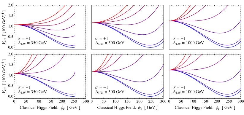
Figure 1: Color online. Variation with respect to temperature $T$ and LW scale $\Lambda_{\rm LW}$ of the LWSM thermal effective potential $V_{\rm eff}(\phi_{c})$. $T$ increases from $0\ \mathrm{GeV}$ (blue, lowest curves) to $300\ \mathrm{GeV}$ (red, highest curves) in increments of $\Delta T=50\ \mathrm{GeV}$.

The LWSM effective potential $V_{\rm eff}^{\rm(1L)}(\phi_{c},T)$ of Eq. (IV.1) is shown in Fig. 1 over a range of temperatures and for different values of the LW scale. In the case $\Lambda_{\text{\sc lw}}=350\ \mathrm{GeV}$, the curves are not drawn for $\phi_{c}\geq\sqrt{4/27}\Lambda_{t}/h_{t}\approx 255\ \mathrm{GeV}$, where the LW stability condition fails in the top sector. The absence of a barrier in the effective potential near the critical temperature implies that the electroweak phase transition is not first order. This conclusion is also illustrated in Fig. 2, where we plot the electroweak order parameter $v(T)$, i.e., the value of $\phi_{c}$ that minimizes the effective potential, versus $T$. We define the phase transition temperature $T_{c}$ by the condition $v(T\geq T_{c})=0$. The absence of a discontinuity in $v(T)$ at $T=T_{c}$ indicates that the phase transition is not first order. In this way, the LWSM electroweak phase transition is similar to the SM phase transition, and in particular implies that LW electroweak baryogenesis is not a viable mechanism for the generation of the baryon asymmetry of the universe Cohen:1993nk .

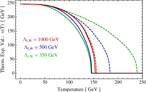
Figure 2: Color online. The electroweak symmetry-breaking order parameter $v(T)$ for the case of $\sigma=+1$ (dashed) and $\sigma=-1$ (solid). Note that the pairs of lines for a given $\Lambda_{\text{\sc lw}}$ move inward monotonically with increasing $\Lambda_{\text{\sc lw}}$. The phase transition temperature is generally higher in the former case due to the cancellation of the leading $O(T^{2})$ temperature dependence discussed in the text.

From Fig. 2 one sees that the limit $\Lambda_{\text{\sc lw}}\gg v$ restores the phase transition temperature to $T_{c}\approx 150\ \mathrm{GeV}$, which corresponds to the SM one-loop result Anderson:1991zb . In the case $\sigma=+1$ ($-1$), the critical temperature is generally larger (smaller). As discussed in Sec. III.3, this result can be understood to arise from cancellations between the positive- and negative-norm fields. To make this cancellation explicit in the LWSM, consider the thermal corrections $\Delta V_{T}^{\rm(1L)}(\phi_{c},T)$ that appear in Eq. (IV.1). For illustrative purposes, one may take the limit $\phi_{c}\ll\Lambda_{\text{\sc lw}}\ll T$, in which all species are light compared to the temperature, and compute

$$\Delta V_{T}^{\rm(1L)}(\phi_{c},T)\approx -\frac{\pi^{2}}{90}g_{\ast}(\sigma)T^{4}$$

$$+T^{2}\times\begin{cases}+\frac{13}{6}\Lambda_{\text{\sc lw}}^{2}&\sigma=+1\,,\\ -\frac{13}{6}\Lambda_{\text{\sc lw}}^{2}+\left(\frac{3g^{2}+g^{\prime\,2}}{16}\!+\!\frac{m_{t}^{2}}{2v^{2}}\!+\!\frac{\lambda}{2}\right)\phi_{c}^{2}+O(\phi_{c}^{4}/\Lambda_{\text{\sc lw}}^{2})&\sigma=-1\,,\end{cases}$$

$$+T\times\begin{cases}+\left(\frac{9g^{2}+3g^{\prime\,2}+3\lambda}{32\pi^{2}}\right)\phi_{c}^{2}\Lambda_{\text{\sc lw}}+O(\phi_{c}^{3}/\Lambda_{\text{\sc lw}})&\sigma=+1\,,\\ -\left(\frac{9g^{2}+3g^{\prime\,2}+3\lambda}{32\pi^{2}}\right)\phi_{c}^{2}\Lambda_{\text{\sc lw}}+O(\phi_{c}^{3}/\Lambda_{\text{\sc lw}})&\sigma=-1\,,\end{cases}$$ (75)

where $g_{\ast}(\sigma)=106.75+197.5\sigma$ is a coefficient recognizing that the LW states contribute negatively to the energy density; it should be interpreted as $106.75$ regular and $197.5$ LW degrees of freedom. Let us consider each term order-by-order in powers of $T$.

The $O(T^{4})$ term has the same form as the free energy density of an ultra-relativistic gas in which all mass scales are negligible and the effective number of degrees of freedom is $g_{\ast}$. Here, the central point of Eqs. (37)-(38), which propagates through Eqs. (III.3.3)-(III.3.3), enters: Each LW degree of freedom contributes a factors $\sigma$ to the potential. The term $g_{\ast}\ni 106.75$ arises from the SM fields, and the larger term $g_{\ast}\ni 197.5\sigma$ arises from the LW fields, which outnumber the SM fields because ($i$) each SM fermion has two LW fermions [Eq. (57)] and ($ii$) the LW gauge bosons have explicit masses. Thus, the sign of $g_{\ast}$ follows the sign of $\sigma$: $g_{\ast}(+1)=304.24$ and $g_{\ast}(-1)=-90.75$. For the case $\sigma=-1$, we find that the free energy density is positive, which implies that the pressure, energy density, and entropy densities are negative. This result has been obtained previously in the context of toy LW theories Fornal:2009xc ; Bhattacharya:2011bb , and its interesting implications have been studied in the context of early universe cosmology Bhattacharya:2012te ; Bhattacharya:2013ut .

In the SM, the term $\Delta V_{T}^{\rm(1L)}\ni T^{2}\,{\rm Tr}\,M^{2}\sim T^{2}\phi_{c}^{2}$ gives rise to symmetry restoration. In the $\sigma=+1$ case, this term is absent due to the cancellation between positive- and negative-norm fields, as already encountered in Sec. III.3. Then symmetry restoration only comes about through the subdominant $O(T\Lambda_{\text{\sc lw}}\phi_{c}^{2})$ term, which results in a higher phase transition temperature. Note that this term only arises by virtue of the $O(T)$ nonanalytic term in the expansion of the bosonic thermal function [see Eq. (65)]. In this case, the fermions are irrelevant for symmetry restoration.

Recently, it has been emphasized Patel:2011th that one must take care in extracting gauge-invariant observables from the manifestly gauge-dependent effective potential Dolan:1973qd . In the conventional phase transition calculation, which we follow here, one obtains $v(T)$ by minimizing $V_{\rm eff}^{(\rm 1L)}$. However this definition of the order parameter endows $v(T)$ with the gauge dependence of the effective potential. In the case of a first-order phase transition, this gauge dependence can lead to anomalous results for observables such as the baryon number preservation criterion and gravity wave spectrum Patel:2011th ; Wainwright:2011qy ; Wainwright:2012zn . However, Garny:2012cg have pointed out that the gauge dependence is small as long as the perturbative expansion is valid. Since the LWSM phase transition is not first order, the only potentially gauge-dependent parameter is $T_{c}$. To check our results, we have also calculated the critical temperature using the technique of Patel:2011th . We find qualitative agreement with the critical temperatures presented in Fig. 2, namely, that $T_{c}$ is generally increased (decreased) for the case $\sigma=+1$ ($-1$) with respect to the SM value, but the gauge-invariant $T_{c}$ is typically O(20-35%) smaller, with the discrepancy at the larger end of this range at lower $\Lambda_{\text{\sc lw}}$. The preceding discussion of the unusual high-temperature behavior of the LWSM is independent of this gauge-fixing ambiguity because the symmetric phase, $\phi_{c}=0$, is a critical point of the effective potential.

For simplicity we have assumed a common LW mass scale $\Lambda_{\text{\sc lw}}\geq 350\ \mathrm{GeV}$ up to this point, but let us now discuss a more phenomenologically motivated parameter set. The strongest constraints on the mass of the LW partners come from electroweak precision tests. The oblique parameter $T$ is sensitive to the LW top, and its constraints impose $\Lambda_{t}>1.5\ \mathrm{TeV}$ at $95\%$ CL Chivukula:2010nw . The oblique parameters $W$ and $Y$ are sensitive to the LW gauge bosons and impose $\Lambda_{W}=\Lambda_{B}>2.3\ \mathrm{TeV}$ at $95\%$ CL Chivukula:2010nw . Finally, the $Z\to b\bar{b}$ branching fraction and forward-backward asymmetry are sensitive to the new charged scalars and impose $\Lambda_{H}>640\ \mathrm{GeV}$ at $95\%$ CL Lebed:2012ab (see also Carone:2009nu ). Setting each of these parameters to its lower bound, we calculate the electroweak order parameter $v(T)$ and find it to be indistinguishable from the solid red (i.e., innermost) curve of Fig. 2. The phase transition temperature is $T_{c}\approx 150\ \mathrm{GeV}$, which is very close to the SM one-loop result (i.e., the $\Lambda_{\text{\sc lw}}\to\infty$ limit). Note that this result is obtained despite the weaker bound on the LW Higgs mass, which presumably could have played a significant role; it suggests that the departures from the SM phase transition seen in Fig. 2 are driven primarily by the LW tops, which at $350\ \mathrm{GeV}$ are near the threshold of their LW stability condition.

V Conclusions

This paper has two goals: to explore the thermodynamics of LW theories and to study the LWSM at temperatures $T\gtrsim O(100-1000\ \mathrm{GeV})$. In a LW theory, the negative-norm degrees of freedom are forbidden from appearing as external states in S-matrix elements by the LW/CLOP prescription, but it is unclear how to implement these constraints when the system is brought to finite temperature. If no special consideration is paid to the negative-norm degrees of freedom, then at leading order in the interactions these LW particles can be treated as a free (ideal) gas, and the partition function is calculated in the standard way. However, it seems that this picture is incompatible with the LW/CLOP prescription. Alternatively, the negative-norm particles can be restricted to internal lines, where they simply modify the energy of the states containing positive-norm SM particles. In the limit of small couplings the LW particles become narrow resonances, but since their decay width is negative (a consequence of the negative-residue propagator), their contribution to the thermodynamic variables is just the opposite of what one would expect for an ideal gas of SM particles. Since some uncertainty remains as to the correct sign of the LW particle contribution to the free energy compared to that of its SM partner, we introduce the index $\sigma=\pm 1$ to consider both cases.

We find that the LWSM electroweak phase transition is qualitatively very similar to the Standard Model crossover. For phenomenologically viable values of the LW mass scale $\Lambda_{\text{\sc lw}}=O({\rm TeV})$, the LW degrees of freedom are heavy and decouple from the physics of the electroweak phase transition that occurs at $T=O(100\ \mathrm{GeV})$. However, at temperatures comparable to $\Lambda_{\text{\sc lw}}$, the LW fields yield significant modifications to the thermodynamics. One finds in case $\sigma=+1$ a cancellation of the leading $O(T^{2})$ correction to the Higgs mass. Since this effective mass is responsible for symmetry restoration, the cancellation tends to retard symmetry restoration and increases the phase transition temperature. In the ultrarelativistic limit, the number of effective species is found to be $g_{\ast}=(106.75+197.5\sigma)$, where the first term is the standard SM contribution and the second term arises from their LW partners, which are greater in number because of the doubling in the fermion sector and explicit gauge boson partner masses. In the case $\sigma=-1$, the LW partners overwhelm the SM degrees of freedom to give $g_{\ast}<0$, implying a negative pressure and energy density.

Our results have immediate implications for early-universe cosmology. Since the electroweak phase transition is not first order, LW electroweak baryogenesis is not a viable explanation for the baryon asymmetry of the universe, nor do we expect other cosmological relics, such as gravitational waves, to be produced. References Bhattacharya:2012te ; Bhattacharya:2013ut studied the effect of LW theories on very early universe cosmology using the case that we call $\sigma=-1$. They find that the unusual thermodynamic properties of LW theories can lead to novel features, such as bouncing cosmologies and mini-reheating events when LW particles decouple. Alternately, if LW thermodynamics is correctly described by the case $\sigma=+1$, then the early-universe cosmology very much resembles the SM concordance model, but with the addition of $197.5$ relativistic degrees of freedom.

An interesting generalization of our work would be to consider the $N=3$ LWSM Carone:2008iw . In that extension, the phenomenological bounds on the LW scale are weaker, and the LW partners may have a more significant impact on the nature of the phase transition. Moreover, many additional degrees of freedom contribute to $g_{\ast}$ and thereby manifest themselves in the high-temperature thermodynamics. Finally, if the narrow-resonance approximation is not valid for some of the LW particles in the LWSM (for any $N$), then a more careful analysis than presented here is required.

Appendix A Quantization Conventions

A.1 Classical to Quantum Theory

A first, essential step to performing calculations with negative-norm states is the establishment of consistent conventions for quantization, time ordering, and the Feynman rules. Since so much potential confusion can arise from improperly handled sign conventions, we begin with the pedagogical exercise of presenting textbook expressions, augmented with the relevant signs. Suppose first that one is given the classical Lagrangian density

$${\cal L}=\eta_{H}\left(\frac{1}{2}\dot{\phi}^{2}-\frac{1}{2}m^{2}\phi^{2}\right)\,,$$ (76)

from which one sees that $\pi_{\phi}\equiv\partial{\cal L}/\partial{\dot{\phi}}=\eta_{H}\dot{\phi}$, and therefore

$${\cal H}=\eta_{H}\left(\frac{1}{2}\pi_{\phi}^{2}+\frac{1}{2}m^{2}\phi^{2}\right)\,.$$ (77)

The sign $\eta_{H}$ is therefore defined so that $\eta_{H}=\pm 1$ gives a semipositive(negative)-definite Hamiltonian density. In order to quantize this theory, one must impose quantization conditions on the fields and their conjugate momenta; however, the sign $\eta_{C}$ of the fundamental commutation relation may be allowed to vary while still allowing unitary time evolution:

$$[\phi(\mathbf{x}),\,\pi_{\phi}(\mathbf{y})]=i\eta_{C}\delta^{(3)}(\mathbf{x}-\mathbf{y})\,.$$ (78)

How does this choice affect the time evolution of states defined on a Hilbert space? For the fundamental field operators $\phi,\,\pi_{\phi}$,

$$\left[\phi,\,H\right] = \eta_{H}\left[\phi(\mathbf{x}),\,\frac{1}{2}\int\!d^{3}\!y\,\pi_{\phi}^{2}(\mathbf{y})\right]=i\eta_{H}\eta_{C}\pi_{\phi}=i\eta_{C}\dot{\phi}\,,$$

$$\left[\pi_{\phi}\,,H\right] = \eta_{H}\left[\pi_{\phi}(\mathbf{x}),\,\frac{1}{2}\,m^{2}\!\!\int d^{3}\!y\,\phi^{2}(\mathbf{y})\right]=-i\eta_{H}\eta_{C}m^{2}\phi=i\eta_{C}\dot{\pi}_{\phi}\,,$$ (79)

which uses the definition of $\pi_{\phi}$, the commutation relation Eq. (78), and the commutator identity $[A,BC]=[A,B]C+B[A,C]$, while the final equality also uses the Hamilton equation of motion, $\dot{\pi}_{\phi}=-\partial{\cal H}/\partial{\phi}=-\eta_{H}m^{2}\phi$. From the above relations, one may prove the more general Heisenberg equation:

$$[\mathcal{O},\,H]=i\eta_{C}\dot{\mathcal{O}}\,,$$ (80)

for any function $\mathcal{O}(\phi,\pi_{\phi})$. The proof is straightforward: Both sides of Eq. (80) are linear in $\mathcal{O}$, so without loss of generality $\mathcal{O}$ may be taken as a monomial in $\phi$ and $\pi_{\phi}$. The commutator identity $[AB,H]=A[B,H]+[A,H]B$ shows that, if $A$ and $B$ separately satisfy Eq. (80), then the right-hand side is $A\dot{B}+B\dot{A}=\dot{(AB)}$, which means that $AB$ also satisfies Eq. (80). Since Eqs. (79) show that $\phi$ and $\pi_{\phi}$ themselves satisfy Eq. (80), then by induction so does any arbitrarily complicated function $\mathcal{O}$ of them. These results indicate that, once the phase space of the system is partitioned into one set for which $\eta_{C}=1$ in Eq. (78) and another set for which $\eta_{C}=-1$, the operators defined in those partitions obey separate Heisenberg equations of motion parameterized by $\eta_{C}$ (and independent of $\eta_{H}$). We do not consider operators that are functions of fields or their conjugate momenta drawn from both partitions.

Now, how does one interpret the potentially “wrong-sign” Heisenberg equations of motion in Eq. (80)? They may be exponentiated to obtain

$$e^{i\eta_{C}H(t-t_{0})}\mathcal{O}(t_{0})e^{-i\eta_{C}H(t-t_{0})}=\mathcal{O}(t)\,.$$ (81)

The fields are therefore evolved forward in time from $t_{0}$ to $t$ by means of the unitary operator $U(t,t_{0})\equiv\mathrm{exp}[-i\eta_{C}H(t-t_{0})]$. For the $\eta_{C}=-1$ partition, this operator has the opposite phase compared to the conventional time evolution operator encountered in quantum field theory. We show next that the choice of $\eta_{C}$ has crucial implications for quantities such as the Feynman propagator of the Lee-Wick field theories, as well as the allowed direction of Wick rotation in the complex $p^{0}$ plane.

A.2 Mode Expansions and the Hamiltonian

We begin with the mode expansions for a Lee-Wick type field $\phi(\mathbf{x})$ and its conjugate momentum $\pi_{\phi}(\mathbf{x})$:

$$\phi(\mathbf{x}) = \int\frac{d^{3}p}{(2\pi)^{3}}\frac{1}{\sqrt{2\omega_{p}}}\left(a_{\mathbf{p}}^{\phantom{\dagger}}e^{i\mathbf{p\cdot x}}+a_{\mathbf{p}}^{\dagger}e^{-i\mathbf{p\cdot x}}\right)=\int\frac{d^{3}p}{(2\pi)^{3}}\frac{1}{\sqrt{2\omega_{p}}}\left(a_{\mathbf{p}}^{\phantom{\dagger}}+a_{\mathbf{-p}}^{\dagger}\right)e^{i\mathbf{p\cdot x}}\,,$$ (82)

$$\pi_{\phi}(\mathbf{x}) = \eta_{H}\int\frac{d^{3}p}{(2\pi)^{3}}(-i)\sqrt{\frac{\omega_{p}}{2}}\left(a_{\mathbf{p}}^{\phantom{\dagger}}e^{i\mathbf{p\cdot x}}-a_{\mathbf{p}}^{\dagger}e^{-i\mathbf{p\cdot x}}\right)$$ (83)

$$= \eta_{H}\int\frac{d^{3}p}{(2\pi)^{3}}(-i)\sqrt{\frac{\omega_{p}}{2}}\left(a_{\mathbf{p}}^{\phantom{\dagger}}-a_{\mathbf{-p}}^{\dagger}\right)e^{i\mathbf{p\cdot x}}\,,$$

where $\omega_{p}\equiv+\sqrt{\mathbf{p}^{2}+m^{2}}$ is strictly positive, and the factor $\eta_{H}$ reflects the result $\pi_{\phi}=\eta_{H}\dot{\phi}$. The canonical commutation relation $[\phi(\mathbf{x}),\pi(\mathbf{y})]=i\eta_{C}\delta^{(3)}(\mathbf{x-y})$ constrains the commutator $[a_{\mathbf{p}}^{\phantom{\dagger}},a_{\mathbf{q}}^{\dagger}]\equiv\eta_{N}(2\pi)^{3}\delta^{(3)}(\mathbf{p-q})$:

$$[\phi(\mathbf{x}),\pi(\mathbf{y})] = -\eta_{H}\int\frac{d^{3}p\,d^{3}q}{(2\pi)^{6}}\frac{i}{2}\sqrt{\frac{\omega_{q}}{\omega_{p}}}\left([a_{\mathbf{-p}}^{\dagger},a_{\mathbf{q}}^{\phantom{\dagger}}]-[a_{\mathbf{p}}^{\phantom{\dagger}},a_{\mathbf{-q}}^{\dagger}]\right)e^{i\mathbf{(p\cdot x+q\cdot y)}}$$ (84)

$$= \eta_{H}\int\frac{d^{3}p\,d^{3}q}{(2\pi)^{6}}\frac{i}{2}\sqrt{\frac{\omega_{q}}{\omega_{p}}}\,2(2\pi)^{3}\eta_{N}\delta^{(3)}(\mathbf{p+q})e^{i(\mathbf{p\cdot x+q\cdot y)}}$$

$$= i\eta_{H}\eta_{N}\delta^{(3)}(\mathbf{x-y})\,,$$

from which one identifies $\eta_{C}=\eta_{H}\eta_{N}$. The interpretation of $\eta_{N}$ becomes apparent once one calculates the spectrum of the theory. The mode expansion of the Hamiltonian reads

$$H = \eta_{H}\int d^{3}x\left[\frac{1}{2}\pi^{2}+\frac{1}{2}(\nabla\phi)^{2}+\frac{1}{2}m^{2}\phi^{2}\right]$$ (85)

$$= \eta_{H}\frac{1}{2}\int d^{3}x\int\frac{d^{3}\!p\,\,d^{3}\!q}{(2\pi)^{6}}e^{i(\mathbf{p+q)\cdot x}}$$

$$\cdot\left[-\frac{\sqrt{\omega_{p}\omega_{q}}}{2}(a_{\mathbf{p}}^{\phantom{\dagger}}-a_{-\mathbf{p}}^{\dagger})(a_{\mathbf{q}}^{\phantom{\dagger}}-a_{-\mathbf{q}}^{\dagger})+\frac{-\mathbf{p\cdot q}+m^{2}}{2\sqrt{\omega_{p}\omega_{q}}}(a_{\mathbf{p}}^{\phantom{\dagger}}+a_{-\mathbf{p}}^{\dagger})(a_{\mathbf{q}}^{\phantom{\dagger}}+a_{-\mathbf{q}}^{\dagger})\right]$$

$$= \eta_{H}\displaystyle\int\frac{d^{3}p}{(2\pi)^{3}}\,\omega_{p}\left(a_{\mathbf{p}}^{\dagger}a_{\mathbf{p}}^{\phantom{\dagger}}+\frac{1}{2}\left[a_{\mathbf{p}},a_{\mathbf{p}}^{\dagger}\right]\right)\,\,.$$

From this expansion follows the commutators:

$$\left[H,a_{\mathbf{p}}^{\phantom{\dagger}}\right] = \eta_{H}\int\frac{d^{3}q}{(2\pi)^{3}}\,\omega_{q}[a_{\mathbf{q}}^{\dagger},a_{\mathbf{p}}^{\phantom{\dagger}}]\,a_{\mathbf{q}}^{\phantom{\dagger}}=-\eta_{H}\eta_{N}\,\omega_{p}\,a_{\mathbf{p}}^{\phantom{\dagger}}=-\eta_{C}\,\omega_{p}\,a_{\mathbf{p}}^{\phantom{\dagger}}\,,$$ (86)

$$\left[H,a_{\mathbf{p}}^{\dagger}\right] = \eta_{H}\int\frac{d^{3}q}{(2\pi)^{3}}\,\omega_{q}\,a_{\mathbf{q}}^{\dagger}[a_{\mathbf{q}}^{\phantom{\dagger}},a_{\mathbf{p}}^{\dagger}]=+\eta_{H}\eta_{N}\,\omega_{p}\,a_{\mathbf{p}}^{\dagger}=+\eta_{C}\,\omega_{p}\,a_{\mathbf{p}}^{\dagger}\,.$$ (87)

These commutation relations immediately provide the time dependence of the ladder operators. Rearranging Eq. (86) into $Ha_{\mathbf{p}}^{\phantom{\dagger}}=a_{\mathbf{p}}^{\phantom{\dagger}}(H-\eta_{C}\omega_{p})$, one acts repeatedly with $H$ on the left to obtain $H^{n}a_{\mathbf{p}}^{\phantom{\dagger}}=a_{\mathbf{p}}^{\phantom{\dagger}}(H-\eta_{C}\omega_{p})^{n}$, which may be exponentiated [consistent with Eq. (81)] to

$$a_{\mathbf{p}}^{\phantom{\dagger}}(t) = U^{\dagger}(t,0)a_{\mathbf{p}}^{\phantom{\dagger}}(t=0)U(t,0)=e^{i\eta_{C}Ht}a_{\mathbf{p}}^{\phantom{\dagger}}e^{-i\eta_{C}Ht}=a_{\mathbf{p}}^{\phantom{\dagger}}e^{-i\omega_{p}t}\,.$$ (88)

Hermitian conjugation of this result immediately gives $a_{\mathbf{p}}^{\dagger}(t)=a_{\mathbf{p}}^{\dagger}\,\mathrm{exp}(i\omega_{p}t)$. In the case $\eta_{H}=-1$, Eqs. (86)–(87) show that the choice $\eta_{N}=-1$ still leads to $a_{\mathbf{p}}^{\dagger}$ and $a_{\mathbf{p}}^{\phantom{\dagger}}$ acting as raising and lowering operators, respectively. One may then define a lowest-energy state $|0\rangle$ such that $a_{\mathbf{p}}^{\phantom{\dagger}}|0\rangle=0$, with single-particle momentum eigenstates $|\mathbf{p}\rangle=\sqrt{2\omega_{p}}\,a_{\mathbf{p}}^{\dagger}|0\rangle$ whose norms are given by

$$\langle\mathbf{p}|\mathbf{q}\rangle=2\sqrt{\omega_{p}\omega_{q}}\langle 0|a_{\mathbf{p}}^{\phantom{\dagger}}a_{\mathbf{q}}^{\dagger}|0\rangle=2\sqrt{\omega_{p}\omega_{q}}\langle 0|[a_{\mathbf{p}}^{\phantom{\dagger}},a_{\mathbf{q}}^{\dagger}]|0\rangle=2\eta_{N}\omega_{p}\,\delta^{(3)}(\mathbf{p-q})\,,$$ (89)

from which one concludes that the $\eta_{N}=-1$ convention corresponds to states of negative norm. In short,

• $\eta_{H}$ is defined by the Hamiltonian (or Lagrangian), (76)-(77);

• $\eta_{C}$ is defined by the $[\phi,\,\pi]$ commutation relation (78);

• $\eta_{N}$ is defined by the $[a^{\phantom{\dagger}},\,a^{\dagger}]$ commutation relation (above (84)) and fixes the norm.

If instead, $\eta_{N}=1$, the spectrum is defined by raising and lowering operators $a_{\mathbf{p}}^{\phantom{\dagger}}$ and $a_{\mathbf{p}}^{\dagger}$, respectively, and one must then define the vacuum in a sensible way. It is possible to choose $a_{\mathbf{p}}^{\dagger}|0\rangle=0$ and build successive $n$-particle states with repeated action of $a_{\mathbf{p}}^{\phantom{\dagger}}$, but this choice effectively amounts just to exchanging the roles of $a_{\mathbf{p}}^{\dagger}$ and $a_{\mathbf{p}}^{\phantom{\dagger}}$. We instead choose the prescription of defining a highest-energy state such that $a_{\mathbf{p}}^{\phantom{\dagger}}|0\rangle=0$, and create negative-energy modes using $|\mathbf{p}\rangle=\sqrt{2\omega_{p}}a_{\mathbf{p}}^{\dagger}|0\rangle$. The Hamiltonian spectrum (ignoring the zero-point energy) for either sign of $\eta_{H}$ then becomes

$$H|\mathbf{p}\rangle = \left(\eta_{H}\int\!\frac{d^{3}q}{(2\pi)^{3}}\,\omega_{q}\,a_{\mathbf{q}}^{\dagger}a_{\mathbf{q}}^{\phantom{\dagger}}\right)a_{\mathbf{p}}^{\dagger}\sqrt{2\omega_{p}}|0\rangle=\eta_{H}\int\frac{d^{3}q}{(2\pi)^{3}}\,\omega_{q}a_{\mathbf{q}}^{\dagger}[a_{\mathbf{q}}^{\phantom{\dagger}},a_{\mathbf{p}}^{\dagger}]\sqrt{2\omega_{p}}|0\rangle$$

$$= \eta_{H}\eta_{N}\omega_{p}a_{\mathbf{p}}^{\dagger}\sqrt{2\omega_{p}}|0\rangle=\eta_{H}\eta_{N}\omega_{p}|\,\mathbf{p}\rangle\,,$$

$$\therefore H|\mathbf{p}\rangle \equiv E_{p}|\mathbf{p}\rangle=\eta_{H}\eta_{N}\omega_{p}|\,\mathbf{p}\rangle=\eta_{C}\omega_{p}|\,\mathbf{p}\rangle\,.$$ (90)

We see that, working in a convention in which there exists a state $\left|0\right>$ annihilated by the operators $a_{\mathbf{p}}^{\phantom{\dagger}}$, the sign $\eta_{C}$ defined in Eq. (78) uniquely determines the sign of the energy eigenvalues. The choice $\eta_{H}=\eta_{C}=\eta_{N}=+1$ is of course the conventional Klein-Gordon theory with positive energies and positive norms, whereas one-particle states in Lee-Wick theories ($\eta_{H}=-1$) can have either negative norms ($\eta_{N}=-1$) and positive energies ($\eta_{C}=+1$) [the conventional formulation] or positive norms ($\eta_{N}=+1$) and negative energies ($\eta_{C}=-1$).

A.3 Calculating the Propagator

For the zero-temperature quantum theory, it is important to define the Feynman propagator so that calculations may be performed in a straightforward manner; to do so relies on how one performs contour integrals in the complex $p^{0}$ plane. This discussion ultimately leads to a proper choice of the $\pm i\epsilon$ terms in the propagator, as well as singling out the unique Wick rotation allowed in defining loop integrals. To begin with, one writes down a mode expansion for the fields generalizing Eq. (82):

$$\phi(x)=\int\frac{d^{3}p}{(2\pi)^{3}}\frac{1}{\sqrt{2\omega_{p}}}\left(a_{\eta_{C}\mathbf{p}}^{\phantom{\dagger}}e^{-ip\cdot x}+a_{\eta_{C}\mathbf{p}}^{\dagger}e^{ip\cdot x}\right)\bigg{|}_{\eta_{C}}\,,$$ (91)

where the $\eta_{C}$ evaluation is shorthand for $p^{0}$ evaluation at $p^{0}=\eta_{C}\omega_{p}=\eta_{H}\eta_{N}\omega_{p}$. This bifurcation admits the possibility of defining the field on either the positive- or negative-mass shell (i.e., $p^{0}=\pm\sqrt{\mathbf{p}^{2}+m^{2}}$). The Lorentz invariance of $p\cdot x$ in Eq. (91) must be maintained in either case, and so we generalize the ladder operators to create and destroy states of momentum $\eta_{C}\mathbf{p}$.

The first step in calculating the Feynman propagator is to obtain the two-point function, $\langle 0|\phi(x)\phi(y)|0\rangle$. For arbitrary $\eta_{N}$, the single non-vanishing term of the transition amplitude is

$$\langle 0|\phi(x)\phi(y)|0\rangle = \int\frac{d^{3}\!p\,d^{3}\!q}{(2\pi)^{6}}\frac{1}{2\sqrt{\omega_{p}\omega_{q}}}\langle 0|a_{\eta_{C}\mathbf{p}}^{\phantom{\dagger}}a_{\eta_{C}\mathbf{q}}^{\dagger}|0\rangle e^{-i(p\cdot x-q\cdot y)}\big{|}_{\eta_{C}}$$ (92)

$$= \int\frac{d^{3}\!p\,d^{3}\!q}{(2\pi)^{3}}\frac{\eta_{N}}{2\sqrt{\omega_{p}\omega_{q}}}\delta^{(3)}[\eta_{C}(\mathbf{p-q})]e^{-i(p\cdot x-q\cdot y)}\big{|}_{\eta_{C}}$$

$$= \int\frac{d^{3}p}{(2\pi)^{3}}\frac{\eta_{N}}{2\omega_{p}}e^{-ip\cdot(x-y)}\big{|}_{\eta_{C}}$$

$$\equiv D^{\eta}(x-y)\,.$$

The superscript $\eta$ serves as a bookkeeping tool to remember which quantization scheme one is using. Now that the form of the two-point function is determined, one constructs the time-ordered Feynman propagator:

$$D_{F}^{\eta}(x-y) \equiv \theta(x^{0}-y^{0})D^{\eta}(x-y)+\theta(y^{0}-x^{0})D^{\eta}(y-x)$$ (93)

$$= \int\frac{d^{3}p}{(2\pi)^{3}}\frac{\eta_{N}}{2\omega_{p}}\left[\theta(x^{0}-y^{0})e^{-ip\cdot(x-y)}\big{|}_{p^{0}=\eta_{C}\omega_{p}}+\theta(y^{0}-x^{0})e^{ip\cdot(x-y)}\big{|}_{p^{0}=\eta_{C}\omega_{p}}\right]$$

$$= \int\frac{d^{3}p}{(2\pi)^{3}}\frac{\eta_{N}}{2\omega_{p}}\left[\theta(x^{0}-y^{0})e^{-ip\cdot(x-y)}\big{|}_{p^{0}=\eta_{C}\omega_{p}}+\theta(y^{0}-x^{0})e^{-ip\cdot(x-y)}\big{|}_{p^{0}=-\eta_{C}\omega_{p}}\right]$$

$$= \int\frac{d^{4}p}{(2\pi)^{3}}\frac{\eta_{N}}{2\omega_{p}}\left[\theta(x^{0}-y^{0})\delta(p^{0}\!-\eta_{C}\omega_{p})+\theta(y^{0}-x^{0})\delta(p^{0}\!+\eta_{C}\omega_{p})\right]e^{-ip\cdot(x-y)}.$$

To continue, we invoke the Lee-Wick prescription: The theory must be free of exponentially growing outgoing modes. This condition determines how the poles are to be pushed above and below the real $p^{0}$ axis as a function of the parameter $\eta_{C}$. Equation (93) may now be rewritten as

$$\int\frac{d^{4}p}{(2\pi)}\frac{\eta_{N}}{2\omega_{p}}[\delta(p^{0}-\eta_{C}\omega_{p}+i\epsilon)+\delta(p^{0}+\eta_{C}\omega_{p}-i\epsilon)]e^{-ip\cdot(x-y)}$$ (94)

$$= \int\frac{d^{4}p}{(2\pi)^{3}}\frac{\eta_{N}}{2\omega_{p}}\left(\frac{1}{-2\pi i}\cdot\frac{1}{p^{0}-(\eta_{C}-i\epsilon)}+\frac{1}{2\pi i}\cdot\frac{1}{p^{0}+(\eta_{C}\omega_{p}-i\epsilon)}\right)e^{-ip\cdot(x-y)}$$

$$= \int\frac{d^{4}p}{(2\pi)^{4}}\frac{i\eta_{N}}{2\omega_{p}}\left(\frac{p^{0}+\eta_{C}\omega_{p}-i\epsilon-p^{0}+\eta_{C}\omega_{p}-i\epsilon}{(p^{0})^{2}-(\eta_{C}\omega_{p}-i\epsilon)^{2}}\right)e^{-ip\cdot(x-y)}$$

$$= \int\frac{d^{4}p}{(2\pi)^{4}}\frac{i\eta_{N}\eta_{C}}{p^{2}-m^{2}+i\eta_{C}\epsilon}e^{-ip\cdot(x-y)},$$

from which one obtains the momentum-space Feynman propagator

$$\tilde{D}^{\eta}_{F}(p)=\frac{i\eta_{H}}{p^{2}-m^{2}+i\eta_{C}\epsilon}\,.$$ (95)

Examining the structure of Eq. (95), one sees that Lee-Wick theories of either quantization possess the hallmark “wrong-sign” propagator, since $\eta_{H}=\eta_{C}\eta_{N}=-1$ for them. The conventional Klein-Gordon propagator may also be recovered upon setting $\eta_{H}=\eta_{C}=\eta_{N}=+1$. However, one subtlety does exist for the case $\eta_{C}=-\eta_{N}=1$: The Feynman prescription for integrating around the poles has the opposite sign with respect to the usual case. This means that the shifted poles lie in the first and third quadrants, rather than the fourth and second; therefore, when one attempts a Wick rotation upon evaluating a loop integral, the proper substitution is $p_{0}=-ip^{0}_{E}$, corresponding to counterclockwise rotation in the complex $p^{0}$ plane.

Appendix B The LWSM Spectrum

For completeness, we present here the calculation of the field-dependent masses that appear in Table 2. We use the metric convention $g_{\mu\nu}={\rm diag}(1,-1,-1,-1)$.

B.1 Higgs & Electroweak Gauge Sector

In the higher-derivative formalism, we denote the Higgs doublet as $\hat{H}$, the $\mathrm{SU}\bigl{(}2\bigr{)}_{L}$ gauge field as $\hat{W}^{a}_{\mu}$, and the $\mathrm{U}\bigl{(}1\bigr{)}_{Y}$ gauge field as $\hat{B}_{\mu}$. We suppose that there is a nonzero homogenous Higgs condensate $\langle\hat{H}\rangle=(0\,,\,\phi_{c}/\sqrt{2})^{T}$ that breaks the electroweak symmetry down to $\mathrm{U}\bigl{(}1\bigr{)}_{\rm EM}$. The Higgs field may be expanded about the background as

$$\hat{H}=\begin{pmatrix}\hat{h}^{+}\\ \frac{\phi_{c}+\hat{h}+i\hat{P}}{\sqrt{2}}\end{pmatrix}\,,$$ (96)

where $\hat{h}$ and $\hat{P}$ are real scalar fields and $\hat{h}^{+}$ is complex. After electroweak symmetry breaking, we denote the photon, neutral weak boson, and charged weak boson fields as $\hat{A}_{\mu}$, $\hat{Z}_{\mu}$, and $\hat{W}^{\pm}_{\mu}$ respectively. These are related to the original electroweak gauge fields by the standard transformations

$$\begin{array}[]{lll}\hat{Z}_{\mu}&=&\cos\theta_{W}\,\hat{W}^{3}_{\mu}-\sin\theta_{W}\,\hat{B}_{\mu}\,,\\ \hat{A}_{\mu}&=&\sin\theta_{W}\,\hat{W}^{3}_{\mu}+\cos\theta_{W}\,\hat{B}_{\mu}\,,\\ \hat{W}^{\pm}_{\mu}&=&\frac{1}{\sqrt{2}}\left(\hat{W}^{1}_{\mu}\mp i\hat{W}^{2}_{\mu}\right)\,,\end{array}$$ (100)

where $\cos\theta_{W}=g/\sqrt{g^{2}+g^{\prime\,2}}$ and $\sin\theta_{W}=g^{\prime}/\sqrt{g^{2}+g^{\prime\,2}}$. We work in the $R_{\xi}$ gauge formalism for generality and restrict to the Landau gauge ($\xi=0$) at the end. We introduce eight anti-commuting, scalar ghost fields $c_{A}$, $c_{Z}$, $c_{W^{+}}$, $c_{W^{-}}$, $\bar{c}_{A}$, $\bar{c}_{Z}$, $\bar{c}_{W^{+}}$, and $\bar{c}_{W^{-}}$.

The gauge-fixed LWSM electroweak sector is specified by the Lagrangian

$$\mathcal{L}_{\rm hd}^{\rm(EW)}=\mathcal{L}_{\rm hd}^{\rm(H)}+\mathcal{L}_{\rm hd}^{\rm(B)}+\mathcal{L}_{\rm hd}^{\rm(W)}+\mathcal{L}_{\rm hd}^{\rm(g.f.)}+\mathcal{L}_{\rm hd}^{\rm(gh.)}\,,$$ (101)

$$\qquad\begin{array}[]{l}\mathcal{L}_{\rm hd}^{\rm(H)}=\left|\hat{D}_{\mu}\hat{H}\right|^{2}-\frac{1}{\Lambda_{H}^{2}}\left|\hat{D}_{\mu}\hat{D}^{\mu}\hat{H}\right|^{2}-U_{\rm hd}(\hat{H})\,,\\ \mathcal{L}_{\rm hd}^{\rm(B)}=-\frac{1}{4}\hat{B}_{\mu\nu}\hat{B}^{\mu\nu}+\frac{1}{2\Lambda_{B}^{2}}\left(\partial^{\mu}\hat{B}_{\mu\nu}\right)^{2}\,,\\ \mathcal{L}_{\rm hd}^{\rm(W)}=-\frac{1}{4}\hat{W}^{a}_{\mu\nu}\hat{W}^{a\,\mu\nu}+\frac{1}{2\Lambda_{W}^{2}}\left(D^{\mu}\hat{W}^{a}_{\mu\nu}\right)^{2}\,,\\ \mathcal{L}_{\rm hd}^{\rm(g.f.)}=-\frac{1}{2\xi_{A}}\left(\partial^{\mu}\hat{A}_{\mu}\right)^{2}-\frac{1}{2\xi_{Z}}\left(\partial^{\mu}\hat{Z}_{\mu}-\xi_{Z}\,\frac{\sqrt{g^{2}+g^{\prime\,2}}}{2}\,\phi_{c}\hat{P}\right)^{2}-\frac{1}{\xi_{W}}\left|\partial^{\mu}\hat{W}^{+}_{\mu}-i\,\xi_{W}\,\frac{g}{2}\,\phi_{c}\hat{h}^{+}\right|^{2}\,,\\ \mathcal{L}_{\rm hd}^{\rm(gh.)}=\bar{c}_{A}(-\partial^{2})c_{A}+\bar{c}_{Z}\left(-\partial^{2}-\xi_{Z}\frac{g^{2}+g^{\prime\,2}}{4}\phi_{c}^{2}\right)c_{Z}+\bar{c}_{W^{+}}\left(-\partial^{2}-\xi_{W}\frac{g^{2}}{4}\phi_{c}^{2}\right)c_{W^{+}}\\ \hskip 56.9055pt+\bar{c}_{W^{-}}\left(-\partial^{2}-\xi_{W}\frac{g^{2}}{4}\phi_{c}^{2}\right)c_{W^{-}}+{\rm interactions}\,,\end{array}$$ (108)

where

$$U_{\rm hd}(\hat{H})=\lambda\left(\hat{H}^{\dagger}\hat{H}-\frac{v^{2}}{2}\right)^{2}\,,$$ (109)

$$\hat{D}_{\mu}H=\left(\partial_{\mu}-ig\frac{\sigma^{a}}{2}\hat{W}_{\mu}^{a}-ig^{\prime}\frac{1}{2}\hat{B}_{\mu}\right)H\,,$$ (110)

$$\hat{B}_{\mu\nu}=\partial_{\mu}\hat{B}_{\nu}-\partial_{\nu}\hat{B}_{\mu}\,,$$ (111)

$$\hat{W}^{a}_{\mu\nu}=\partial_{\mu}\hat{W}^{a}_{\nu}-\partial_{\nu}\hat{W}^{a}_{\mu}+g\epsilon^{abc}\hat{W}_{\mu}^{b}\hat{W}_{\nu}^{c}\,,$$ (112)

$$(D^{\mu}\hat{W}_{\mu\nu})^{a}=\partial^{\mu}\hat{W}^{a}_{\mu\nu}+g\epsilon^{abc}\hat{W}^{b\,\mu}\hat{W}_{c\,\mu\nu}\ .$$ (113)

Since we are only interested in calculating the tree-level masses, we drop the interactions (terms containing products of three or more fields). After expanding the Higgs field with Eq. (96) and performing the rotation Eq. (100), the Lagrangian becomes

$$U_{\rm hd}=\frac{\lambda}{4}(\phi_{c}^{2}-v^{2})^{2}+\lambda\phi_{c}(\phi_{c}^{2}-v^{2})\hat{h}+\frac{1}{2}\lambda(3\phi_{c}^{2}-v^{2})\hat{h}^{2}+\frac{1}{2}\lambda(\phi_{c}^{2}-v^{2})\hat{P}^{2}+\lambda(\phi_{c}^{2}-v^{2})\hat{h}^{+}\hat{h}^{-}\,,$$ (114)

$$\mathcal{L}_{\rm hd}^{\rm(H)}+\mathcal{L}_{\rm hd}^{\rm(g.f.)}=\frac{1}{2}\left[\left(\partial_{\mu}\hat{h}\right)^{2}-\frac{1}{\Lambda_{H}^{2}}(\partial^{2}\hat{h})^{2}\right]+\frac{1}{2}\left[\left(\partial_{\mu}\hat{P}\right)^{2}-\frac{1}{\Lambda_{H}^{2}}(\partial^{2}\hat{P})^{2}\right]$$

$$\hskip 85.35826pt+\left[\left|\partial_{\mu}\hat{h}^{+}\right|^{2}-\frac{1}{\Lambda_{H}^{2}}\left|\partial^{2}\hat{h}^{+}\right|^{2}\right]$$

$$\hskip 62.59596pt+\frac{1}{2}\frac{g^{2}+g^{\prime\,2}}{4}\phi_{c}^{2}\hat{Z}_{\mu}\hat{Z}^{\mu}+\frac{g^{2}}{4}\phi_{c}^{2}\left|\hat{W}_{\mu}^{-}\right|^{2}-\frac{1}{2}\frac{g^{2}+g^{\prime\,2}}{4}\xi_{Z}\phi_{c}^{2}\hat{P}^{2}-\xi_{W}\frac{g^{2}}{4}\phi_{c}^{2}\left|\hat{h}^{+}\right|^{2}$$

$$\hskip 62.59596pt-\frac{1}{2\xi_{A}}(\partial_{\mu}\hat{A}^{\mu})^{2}-\frac{1}{\xi_{W}}\left|\partial_{\mu}\hat{W}^{-\,\mu}\right|^{2}-\frac{1}{2\xi_{Z}}(\partial_{\mu}\hat{Z}^{\mu})^{2}$$

$$\hskip 62.59596pt+\frac{\sqrt{g^{2}+g^{\prime\,2}}}{2}\phi_{c}\partial_{\mu}\left(\hat{P}\hat{Z}^{\mu}\right)+\frac{g}{2}\phi_{c}\partial_{\mu}\left(i\,\hat{h}^{+}\hat{W}^{-\mu}-i\,\hat{h}^{-}\hat{W}^{+\,\mu}\right)\,,$$ (115)

$$\mathcal{L}_{\rm hd}^{\rm(B)}+\mathcal{L}_{\rm hd}^{\rm(W)}=-\frac{1}{4}\left(\partial_{\mu}\hat{A}_{\nu}-\partial_{\nu}\hat{A}_{\mu}\right)^{2}-\frac{1}{4}\left(\partial_{\mu}\hat{Z}_{\nu}-\partial_{\nu}\hat{Z}_{\mu}\right)^{2}-\frac{1}{2}\left|\partial_{\mu}\hat{W}^{-}_{\nu}-\partial_{\nu}\hat{W}^{-}_{\mu}\right|^{2}$$

$$\hskip 62.59596pt+\frac{1}{\Lambda_{W}^{2}}\left|\partial^{2}\hat{W}_{\mu}^{-}-\partial_{\mu}\partial^{\nu}\hat{W}_{\nu}^{-}\right|^{2}+\frac{1}{2\Lambda_{Z}^{2}}\left(\partial^{2}\hat{Z}_{\mu}-\partial_{\mu}\partial^{\nu}\hat{Z}_{\nu}\right)^{2}$$

$$\hskip 62.59596pt+\frac{1}{2\Lambda_{A}^{2}}\left(\partial^{2}\hat{A}_{\mu}-\partial_{\mu}\partial^{\nu}\hat{A}_{\nu}\right)^{2}-\frac{1}{2\Lambda_{AZ}^{2}}\left(\partial^{2}\hat{A}_{\mu}-\partial_{\mu}\partial^{\nu}\hat{A}_{\nu}\right)\left(\partial^{2}\hat{Z}^{\mu}\!-\partial^{\mu}\partial^{\alpha}\hat{Z}_{\alpha}\right),$$ (116)

where we have defined

$$\begin{array}[]{l}\Lambda_{A}\equiv\left(\frac{\cos^{2}\theta_{W}}{\Lambda_{B}^{2}}+\frac{\sin^{2}\theta_{W}}{\Lambda_{W}^{2}}\right)^{-1/2}\,,\\ \Lambda_{Z}\equiv\left(\frac{\sin^{2}\theta_{W}}{\Lambda_{B}^{2}}+\frac{\cos^{2}\theta_{W}}{\Lambda_{W}^{2}}\right)^{-1/2}\,,\\ \Lambda_{AZ}\equiv\left(\frac{\sin 2\theta_{W}}{\Lambda_{B}^{2}}-\frac{\sin 2\theta_{W}}{\Lambda_{W}^{2}}\right)^{-1/2}\,.\end{array}$$ (120)

The final two terms in Eq. (115) are total derivatives and can be dropped. After integrating by parts and dropping total derivative terms, one obtains

$$\mathcal{L}_{\rm hd}^{\rm(EW)}= -\frac{\lambda}{4}(\phi_{c}^{2}-v^{2})^{2}-\lambda\phi_{c}(\phi_{c}^{2}-v^{2})\hat{h}$$ (121)

$$+\frac{1}{2}\hat{h}\left(-\partial^{2}-\frac{1}{\Lambda_{H}^{2}}\partial^{4}-{m}^{2}_{\hat{h}}\right)\hat{h}+\frac{1}{2}\hat{P}\left(-\partial^{2}-\frac{1}{\Lambda_{H}^{2}}\partial^{4}-{m}^{2}_{\hat{P}}\right)\hat{P}$$

$$\hskip 28.45274pt+\hat{h}^{+}\left(-\partial^{2}-\frac{1}{\Lambda_{H}^{2}}\partial^{4}-{m}^{2}_{\hat{h}^{\pm}}\right)\hat{h}^{-}$$

$$+\frac{1}{2}\hat{A}^{\mu}\left[-g_{\mu\nu}\left(-\partial^{2}-\frac{\partial^{4}}{\Lambda_{A}^{2}}-{m}^{2}_{\hat{A}}\right)+\left(-\frac{\partial^{2}}{\Lambda_{A}^{2}}-1+\frac{1}{\xi_{A}}\right)\partial_{\mu}\partial_{\nu}\right]\hat{A}^{\nu}$$

$$+\frac{1}{2}\hat{Z}^{\mu}\left[-g_{\mu\nu}\left(-\partial^{2}-\frac{\partial^{4}}{\Lambda_{Z}^{2}}-{m}^{2}_{\hat{Z}}\right)+\left(-\frac{\partial^{2}}{\Lambda_{Z}^{2}}-1+\frac{1}{\xi_{Z}}\right)\partial_{\mu}\partial_{\nu}\right]\hat{Z}^{\nu}$$

$$+\frac{1}{2}\hat{A}^{\mu}\left[-\left(g_{\mu\nu}\partial^{2}-\partial_{\mu}\partial_{\nu}\right)\frac{\partial^{2}}{\Lambda_{AZ}^{2}}\right]\hat{Z}^{\nu}$$

$$+\hat{W}^{+\,\mu}\left[-g_{\mu\nu}\left(-\partial^{2}-\frac{\partial^{4}}{\Lambda_{W}^{2}}-{m}^{2}_{\hat{W}^{\pm}}\right)+\left(-\frac{\partial^{2}}{\Lambda_{W}^{2}}-1+\frac{1}{\xi_{W}}\right)\partial_{\mu}\partial_{\nu}\right]\hat{W}^{-\,\nu}$$

$$+\bar{c}_{A}(-\partial^{2})c_{A}+\bar{c}_{Z}\left(-\partial^{2}-\xi_{Z}{m}_{\hat{Z}}^{2}\right)c_{Z}+\bar{c}_{W^{+}}\left(-\partial^{2}-\xi_{W}{m}_{\hat{W}^{\pm}}^{2}\right)c_{W^{+}}$$

$$\hskip 28.45274pt+\bar{c}_{W^{-}}\left(-\partial^{2}-\xi_{W}{m}_{\hat{W}^{\pm}}^{2}\right)c_{W^{-}}\,,$$ (122)

where

$$\begin{array}[]{lll}{m}_{\hat{h}}^{2}&\equiv&\lambda(3\phi_{c}^{2}-v^{2})\,,\\ {m}_{\hat{P}}^{2}&\equiv&\lambda(\phi_{c}^{2}-v^{2})+\xi_{Z}{m}_{\hat{Z}}^{2}\,,\\ {m}_{\hat{h}^{\pm}}^{2}&\equiv&\lambda(\phi_{c}^{2}-v^{2})+\xi_{W}{m}_{\hat{Z}}^{2}\,,\end{array}\hskip 56.9055pt\begin{array}[]{lll}{m}_{\hat{W}^{\pm}}^{2}&\equiv&\frac{g^{2}}{4}\phi_{c}^{2}\,,\\ {m}_{\hat{Z}}^{2}&\equiv&\frac{g^{2}+g^{\prime\,2}}{4}\phi_{c}^{2}\,,\\ {m}_{\hat{A}}^{2}&\equiv&0\,.\\ \end{array}$$ (129)

With the Lagrangian in this form, it is straightforward to read off the propagators. For the scalars one finds

$$D_{\hat{h}}(p)=i\left(p^{2}-\frac{p^{4}}{\Lambda_{H}^{2}}-{m}_{\hat{h}}^{2}\right)^{-1}=\frac{\Lambda_{H}^{2}}{{m}_{\tilde{h}}^{2}-{m}_{h}^{2}}\left(\frac{i}{p^{2}-{m}_{h}^{2}}-\frac{i}{p^{2}-{m}_{\tilde{h}}^{2}}\right)\,,$$

$$D_{\hat{P}}(p)=i\left(p^{2}-\frac{p^{4}}{\Lambda_{H}^{2}}-{m}_{\hat{P}}^{2}\right)^{-1}=\frac{\Lambda_{H}^{2}}{{m}_{\tilde{P}}^{2}-{m}_{P}^{2}}\left(\frac{i}{p^{2}-{m}_{P}^{2}}-\frac{i}{p^{2}-{m}_{\tilde{P}}^{2}}\right)\,,$$

$$D_{\hat{h}^{\pm}}(p)=i\left(p^{2}-\frac{p^{4}}{\Lambda_{H}^{2}}-{m}_{\hat{h}^{\pm}}^{2}\right)^{-1}=\frac{\Lambda_{H}^{2}}{{m}_{\tilde{h}^{\pm}}^{2}-{m}_{h^{\pm}}^{2}}\left(\frac{i}{p^{2}-{m}_{h^{\pm}}^{2}}-\frac{i}{p^{2}-{m}_{\tilde{h}^{\pm}}^{2}}\right)\,,$$ (130)

where

$$\begin{array}[]{lll}&&\text{SM-like Pole}\\ {m}_{h}^{2}&=&\frac{\Lambda_{H}^{2}}{2}\left(1-\sqrt{1-\frac{4{m}_{\hat{h}}^{2}}{\Lambda_{H}^{2}}}\right)\,,\\ {m}_{P}^{2}&=&\frac{\Lambda_{H}^{2}}{2}\left(1-\sqrt{1-\frac{4{m}_{\hat{P}}^{2}}{\Lambda_{H}^{2}}}\right)\,,\\ {m}_{h^{\pm}}^{2}&=&\frac{\Lambda_{H}^{2}}{2}\left(1-\sqrt{1-\frac{4{m}_{\hat{h}^{\pm}}^{2}}{\Lambda_{H}^{2}}}\right)\,,\end{array}\hskip 56.9055pt\begin{array}[]{lll}&&\text{LW-like Pole}\\ {m}_{\tilde{h}}^{2}&=&\frac{\Lambda_{H}^{2}}{2}\left(1+\sqrt{1-\frac{4{m}_{\hat{h}}^{2}}{\Lambda_{H}^{2}}}\right)\,,\\ {m}_{\tilde{P}}^{2}&=&\frac{\Lambda_{H}^{2}}{2}\left(1+\sqrt{1-\frac{4{m}_{\hat{P}}^{2}}{\Lambda_{H}^{2}}}\right)\,,\\ {m}_{\tilde{h}^{\pm}}^{2}&=&\frac{\Lambda_{H}^{2}}{2}\left(1+\sqrt{1-\frac{4{m}_{\hat{h}^{\pm}}^{2}}{\Lambda_{H}^{2}}}\right)\,.\end{array}$$ (139)

The poles are classified as “SM-like” or “LW-like”, depending on whether the residue of the pole is positive or negative.

In the gauge sector, the ghost propagators are immediately seen to be

$$\begin{array}[]{l}D_{c_{A}}(p)=\frac{i}{p^{2}}\,,\\ D_{c_{Z}}(p)=\frac{i}{p^{2}-\xi_{Z}\,m_{\hat{Z}}^{2}}\,,\\ D_{c_{W^{+}}}(p)=\frac{i}{p^{2}-\xi_{W}\,m_{\hat{W}^{\pm}}^{2}}\,,\\ D_{c_{W^{-}}}(p)=\frac{i}{p^{2}-\xi_{W}\,m_{\hat{W}^{\pm}}^{2}}\,.\end{array}$$ (144)

We define the transverse and longitudinal projection operators $\Pi_{T}^{\mu\nu}\equiv g^{\mu\nu}-p^{\mu}p^{\nu}/p^{2}$ and $\Pi_{L}^{\mu\nu}\equiv p^{\mu}p^{\nu}/p^{2}$, and obtain

$$D^{\mu\nu}_{\hat{W}^{\pm}}(p)= -i\,\Pi_{T}^{\mu\nu}(p)\left(p^{2}-\frac{p^{4}}{\Lambda_{W}^{2}}-{m}_{\hat{W}^{\pm}}^{2}\right)^{-1}-i\,\Pi_{L}^{\mu\nu}(p)\left(\frac{p^{2}}{\xi_{W}}-{m}_{\hat{W}^{\pm}}^{2}\right)^{-1}$$

$$= \frac{\Lambda_{W}^{2}}{{m}_{\tilde{W}^{\pm}}^{2}-{m}_{W^{\pm}}^{2}}\left(\frac{-i\,\Pi^{\mu\nu}_{T}(p)}{p^{2}-{m}_{W^{\pm}}^{2}}-\frac{-i\,\Pi^{\mu\nu}_{T}(p)}{p^{2}-{m}_{\tilde{W}^{\pm}}^{2}}\right)+\frac{-i\,\xi_{W}\,\Pi^{\mu\nu}_{L}(p)}{p^{2}-\xi_{W}{m}_{\hat{W}^{\pm}}^{2}}\,,$$ (145)

where

$$\begin{array}[]{lll}&&\text{SM-like Pole}\\ {m}_{W^{\pm}}^{2}&=&\frac{\Lambda_{W}^{2}}{2}\left(1-\sqrt{1-\frac{4{m}_{\hat{W}^{\pm}}^{2}}{\Lambda_{W}^{2}}}\right)\,,\end{array}\hskip 56.9055pt\begin{array}[]{lll}&&\text{LW-like Pole}\\ {m}_{\tilde{W}^{\pm}}^{2}&=&\frac{\Lambda_{W}^{2}}{2}\left(1+\sqrt{1-\frac{4{m}_{\hat{W}^{\pm}}^{2}}{\Lambda_{W}^{2}}}\right)\,.\end{array}$$ (150)

We defer a discussion of the longitudinal polarization state until the end. The term on line Eq. (B.1) corresponds to a mixing between transverse polarizations of $\hat{A}^{\mu}$ and $\hat{Z}^{\mu}$, which gives rise to off-diagonal terms in the inverse propagator:

$$(D_{\hat{A}\hat{Z}}^{-1})^{\mu\nu}(p)=i\,\Pi_{T}^{\mu\nu}\begin{pmatrix}p^{2}-\frac{p^{4}}{\Lambda_{A}^{2}}-{m}_{\hat{A}}^{2}&\frac{p^{4}}{2\Lambda_{AZ}^{2}}\\ \frac{p^{4}}{2\Lambda_{AZ}^{2}}&p^{2}-\frac{p^{4}}{\Lambda_{Z}^{2}}-{m}_{\hat{Z}}^{2}\end{pmatrix}+i\,\Pi_{L}^{\mu\nu}\begin{pmatrix}\frac{p^{2}}{\xi_{A}}-{m}_{\hat{A}}^{2}&0\\ 0&\frac{p^{2}}{\xi_{Z}}-{m}_{\hat{Z}}^{2}\end{pmatrix}\ .$$ (151)

For simplicity, we assume just one common LW scale in the EW gauge sector. Then one has $\Lambda_{B}=\Lambda_{W}=\Lambda_{A}=\Lambda_{Z}\equiv\Lambda_{\rm EW}$ and also $(\Lambda_{AZ})^{-2}=0$ using Eq. (120). The mixing vanishes and the propagators become

$$D^{\mu\nu}_{\hat{A}}(p)= \frac{\Lambda_{\rm EW}^{2}}{{m}_{\tilde{A}}^{2}-{m}_{A}^{2}}\left(\frac{-i\,\Pi^{\mu\nu}_{T}(p)}{p^{2}-{m}_{A}^{2}}-\frac{-i\,\Pi^{\mu\nu}_{T}(p)}{p^{2}-{m}_{\tilde{A}}^{2}}\right)+\frac{-i\,\xi_{A}\,\Pi^{\mu\nu}_{L}(p)}{p^{2}-\xi_{A}{m}_{\hat{A}}^{2}}\,,$$ (152)

$$D^{\mu\nu}_{\hat{Z}}(p)= \frac{\Lambda_{\rm EW}^{2}}{{m}_{\tilde{Z}}^{2}-{m}_{Z}^{2}}\left(\frac{-i\,\Pi^{\mu\nu}_{T}(p)}{p^{2}-{m}_{Z}^{2}}-\frac{-i\,\Pi^{\mu\nu}_{T}(p)}{p^{2}-{m}_{\tilde{Z}}^{2}}\right)+\frac{-i\,\xi_{Z}\,\Pi^{\mu\nu}_{L}(p)}{p^{2}-\xi_{Z}{m}_{\hat{Z}}^{2}}\,,$$ (153)

where

$$\begin{array}[]{lll}&&\text{SM-like Pole}\\ {m}_{A}^{2}&=&\frac{\Lambda_{\rm EW}^{2}}{2}\left(1-\sqrt{1-\frac{4{m}_{\hat{A}}^{2}}{\Lambda_{\rm EW}^{2}}}\right)=0\,,\\ {m}_{Z}^{2}&=&\frac{\Lambda_{\rm EW}^{2}}{2}\left(1-\sqrt{1-\frac{4{m}_{\hat{Z}}^{2}}{\Lambda_{\rm EW}^{2}}}\right)\,,\end{array}\hskip 42.67912pt\begin{array}[]{lll}&&\text{LW-like Pole}\\ {m}_{\tilde{A}}^{2}&=&\frac{\Lambda_{\rm EW}^{2}}{2}\left(1+\sqrt{1-\frac{4{m}_{\hat{A}}^{2}}{\Lambda_{\rm EW}^{2}}}\right)=\Lambda_{\rm EW}^{2}\,,\\ {m}_{\tilde{Z}}^{2}&=&\frac{\Lambda_{\rm EW}^{2}}{2}\left(1+\sqrt{1-\frac{4{m}_{\hat{Z}}^{2}}{\Lambda_{\rm EW}^{2}}}\right)\,.\end{array}$$ (160)

Note that the photon is massless, and that the mass of its LW partner is independent of $\phi_{c}$.

Having calculated the spectrum, let us discuss the counting of degrees of freedom. The scalar propagators Eq. (B.1) reveal that each of the fields $\hat{h},\hat{P},\hat{h}^{+},$ and $\hat{h}^{-}$ carries two degrees of freedom: a lighter SM-like resonance and a heavier LW-like resonance. We might expect this doubling to carry over to the gauge fields as well, but an inspection of their propagators reveals that this is not the case. In counting the gauge boson degrees of freedom, note that ${\rm Tr}\,\Pi_{T}=\Pi_{T,\,\mu\nu}g^{\mu\nu}=3$ and ${\rm Tr}\,\Pi_{L}=1$. Examining the propagator Eq. (152), we see that the $\hat{A}$ contains seven degrees of freedom: three massless transverse polarizations (${m}_{A}^{2}=0$), one massless longitudinal polarization (${m}_{\hat{A}}^{2}=0$), and three massive transverse polarizations (${m}_{\tilde{A}}^{2}=\Lambda_{\rm EW}^{2}$). The four massless degrees of freedom constitute the SM photon, and after accounting for the two “negative degrees of freedom” of the ghosts $c_{A}$ and $\bar{c}_{A}$, the count of “physical” photon polarizations is reduced to two. Here, the LWSM does not double the number of gauge degrees of freedom, but instead adds three, which is what one expects for an additional massive resonance. For the $\hat{Z}$ boson we count three degrees of freedom with mass ${m}_{Z}^{2}$, three degrees of freedom with mass ${m}_{\tilde{Z}}^{2}$, one degree of freedom with mass $\xi_{Z}\,{m}_{\hat{Z}}^{2}$, and two negative degrees of freedom of mass $\xi_{Z}\,{m}_{\hat{Z}}^{2}$ coming from the ghosts. The ghost cancels the longitudinal polarization state, and one negative degree of freedom remains. Once we restrict to the Landau gauge ($\xi_{A}=\xi_{Z}=\xi_{W}=0$), the ghosts and longitudinal polarizations become massless. Then these degrees of freedom do not yield a field-dependent contribution to the effective potential, but they do affect the number of relativistic species at finite temperature. Thus, we have counted them as massless particles in Table 2, which also summarizes Eqs. (139), (150), and (160).

B.2 Top Sector

Let the $\mathrm{SU}\bigl{(}2\bigr{)}$ doublet $\hat{Q}_{L}=(\hat{u}_{L}\,,\,\hat{d}_{L})^{T}$ be a left-handed Weyl spinor, and let the singlet $\hat{u}_{R}$ be a right-handed Weyl spinor. Neglecting gauge interactions, the Lagrangian for the top sector is written as

$$\mathcal{L}_{\rm hd}^{\rm(top)}=\, (\hat{Q}_{L})^{\dagger}i\bar{\not{\partial}}\hat{Q}_{L}+\frac{1}{\Lambda_{Q}^{2}}(\hat{Q}_{L})^{\dagger}i\bar{\not{\partial}}\not{\partial}\bar{\not{\partial}}\hat{Q}_{L}+(\hat{u}_{R})^{\dagger}i\not{\partial}\hat{u}_{R}+\frac{1}{\Lambda_{u}^{2}}(\hat{u}_{R})^{\dagger}i\not{\partial}\bar{\not{\partial}}\not{\partial}\hat{u}_{R}\,,$$

$$-h_{t}\left((\hat{Q}_{L})^{\dagger}{\bm{\epsilon}}\hat{H}^{\ast}\hat{u}_{R}-(\hat{u}_{R})^{\dagger}\hat{H}{\bm{\epsilon}}\hat{Q}_{L}\right)\,,$$ (161)

where $\not{\partial}=\sigma^{\mu}\partial_{\mu}$ and $\bar{\not{\partial}}=\bar{\sigma}^{\mu}\partial_{\mu}$. Contractions of the $\mathrm{SU}\bigl{(}2\bigr{)}$ doublets is accomplished with the totally antisymmetric 2-tensor ${\bm{\epsilon}}$. After electroweak symmetry breaking, one replaces $\hat{H}\to(0\,,\,\phi_{c}/\sqrt{2})^{T}$, and obtains

$$\mathcal{L}_{\rm hd}^{\rm(top)}=\, (\hat{u}_{L})^{\dagger}\left(i\bar{\not{\partial}}+\frac{i\bar{\not{\partial}}\not{\partial}\bar{\not{\partial}}}{\Lambda_{Q}^{2}}\right)\hat{u}_{L}+(\hat{u}_{R})^{\dagger}\left(i\not{\partial}+\frac{i\not{\partial}\bar{\not{\partial}}\not{\partial}}{\Lambda_{u}^{2}}\right)\hat{u}_{R}-\frac{h_{t}\,\phi_{c}}{\sqrt{2}}\left[(\hat{u}_{L})^{\dagger}\hat{u}_{R}+(\hat{u}_{R})^{\dagger}\hat{u}_{L}\right]\ .$$ (162)

One can now collect the Weyl spinors into the Dirac spinor $\hat{t}=(\,\hat{u}_{L}\,,\,\hat{u}_{R}\,)^{T}$. Using the standard definitions

$$\gamma^{\mu}=\left(\begin{smallmatrix}0&\sigma^{\mu}\\ \bar{\sigma}^{\mu}&0\end{smallmatrix}\right)\hskip 11.38092pt,\hskip 11.38092pt\bar{\hat{t}}\equiv\hat{t}^{\dagger}\gamma^{0}\hskip 11.38092pt,\hskip 11.38092pt\not{\partial}\hat{t}=\gamma^{\mu}\partial_{\mu}\hat{t}\hskip 11.38092pt,\hskip 11.38092pt\gamma^{5}=i\gamma^{0}\gamma^{1}\gamma^{2}\gamma^{3}\hskip 11.38092pt,\hskip 11.38092ptP_{L,R}=\frac{1\mp\gamma^{5}}{2}\ \ ,$$

the Lagrangian can be written as

$$\mathcal{L}_{\rm hd}^{\rm(top)}=\bar{\hat{t}}\left(i\not{\partial}+\frac{i\not{\partial}^{3}}{\Lambda_{Q}^{2}}P_{L}+\frac{i\not{\partial}^{3}}{\Lambda_{u}^{2}}P_{R}\right)\hat{t}-\bar{\hat{t}}{m}_{\hat{t}}\hat{t}\,,$$ (163)

where ${m}_{\hat{t}}\equiv h_{t}\phi_{c}/\sqrt{2}$. To simplify, we assume that $\Lambda_{Q}=\Lambda_{u}\equiv\Lambda_{t}$. Then the Lagrangian reduces to Eq. (52), and the propagator is

$$D_{\hat{t}}(p)=\ i\left(-\frac{\not{p}^{3}}{\Lambda_{t}^{2}}+\not{p}-{m}_{\hat{t}}(\phi_{c})\right)^{-1}$$

$$=\ +\frac{\Lambda_{t}^{2}}{({m}_{\tilde{t}_{1}}-{m}_{t})({m}_{t}-{m}_{\tilde{t}_{2}})}\frac{i}{\not{p}-{m}_{t}}$$

$$-\frac{\Lambda_{t}^{2}}{({m}_{\tilde{t}_{1}}-{m}_{t})({m}_{\tilde{t}_{1}}-{m}_{\tilde{t}_{2}})}\frac{i}{\not{p}-{m}_{\tilde{t}_{1}}}$$

$$-\frac{\Lambda_{t}^{2}}{({m}_{t}-{m}_{\tilde{t}_{2}})({m}_{\tilde{t}_{1}}-{m}_{\tilde{t}_{2}})}\frac{i}{\not{p}-{m}_{\tilde{t}_{2}}}\,,$$ (164)

where

$$\begin{array}[]{lcl}\text{SM-like Pole:}&&{m}_{t}(\phi_{c})\equiv\Lambda_{t}\sqrt{\frac{2}{3}\left(1-\cos\frac{\theta_{t}}{3}\right)}\,,\\ \text{LW-like Pole:}&&{m}_{\tilde{t}_{1}}(\phi_{c})\equiv\Lambda_{t}\sqrt{\frac{2}{3}\left(1+\cos\frac{\theta_{t}+\pi}{3}\right)}\,,\\ \text{LW-like Pole:}&&{m}_{\tilde{t}_{2}}(\phi_{c})\equiv-\Lambda_{t}\sqrt{\frac{2}{3}\left(1+\cos\frac{\theta_{t}-\pi}{3}\right)}\,,\end{array}$$ (168)

where $\theta_{t}\equiv\arctan\,\frac{2\sqrt{\alpha(1-\alpha)}}{1-2\alpha}$ and $\alpha\equiv\frac{27}{4}\frac{{m}_{\hat{t}}^{2}}{\Lambda_{t}^{2}}$. The angle $0\leq\theta_{t}\leq\pi$ is in the first or second quadrant, and the LW stability condition imposes $\alpha<1$.

References

• (1) B. Grinstein, D. O’Connell, and M. B. Wise, The Lee-Wick standard model, Phys.Rev. D77 (2008) 025012, [arXiv:0704.1845].
• (2) C. D. Carone and R. F. Lebed, Minimal Lee-Wick Extension of the Standard Model, Phys.Lett. B668 (2008) 221–225, [arXiv:0806.4555].
• (3) D. Comelli and J. Espinosa, Bosonic thermal masses in supersymmetry, Phys.Rev. D55 (1997) 6253–6263, [hep-ph/9606438].
• (4) B. Fornal, B. Grinstein, and M. B. Wise, Lee-Wick Theories at High Temperature, Phys.Lett. B674 (2009) 330–335, [arXiv:0902.1585].
• (5) J. R. Espinosa and B. Grinstein, Ultraviolet Properties of the Higgs Sector in the Lee-Wick Standard Model, Phys.Rev. D83 (2011) 075019, [arXiv:1101.5538].
• (6) S. Hawking, Who’s Afraid of (Higher Derivative) Ghosts?, in Quantum Field Theory and Quantum Statistics: Essays in Honor of the 60th Birthday of E.S. Fradkin (A. Batalin, C. Isham, and C. Vilkovisky, eds.). 1985.
• (7) S. Hawking and T. Hertog, Living with ghosts, Phys.Rev. D65 (2002) 103515, [hep-th/0107088].
• (8) T. Lee and G. Wick, Negative Metric and the Unitarity of the S Matrix, Nucl.Phys. B9 (1969) 209–243.
• (9) T. Lee and G. Wick, Finite Theory of Quantum Electrodynamics, Phys.Rev. D2 (1970) 1033–1048.
• (10) R. Cutkosky, P. Landshoff, D. I. Olive, and J. Polkinghorne, A non-analytic S matrix, Nucl.Phys. B12 (1969) 281–300.
• (11) K. Bhattacharya and S. Das, Thermodynamics of the Lee-Wick partners: An alternative approach, Phys.Rev. D84 (2011) 045023, [arXiv:1108.0483].
• (12) W. Pauli, On dirac’s new method of field quantization, Rev. Mod. Phys. 15 (Jul, 1943) 175–207.
• (13) D. G. Boulware and D. J. Gross, Lee-Wick Indefinite Metric Quantization: A Functional Integral Approach, Nucl.Phys. B233 (1984) 1.
• (14) C. D. Carone and R. F. Lebed, A Higher-Derivative Lee-Wick Standard Model, JHEP 0901 (2009) 043, [arXiv:0811.4150].
• (15) B. Grinstein and D. O’Connell, One-Loop Renormalization of Lee-Wick Gauge Theory, Phys.Rev. D78 (2008) 105005, [arXiv:0801.4034].
• (16) C. D. Carone, Higher-Derivative Lee-Wick Unification, Phys.Lett. B677 (2009) 306–310, [arXiv:0904.2359].
• (17) M. Dias, A. Y. Petrov, J. Senise, C.R., and A. da Silva, Effective potential for a SUSY Lee-Wick model: the Wess-Zumino case, arXiv:1212.5220.
• (18) F. Gama, M. Gomes, J. Nascimento, A. Y. Petrov, and A. da Silva, On the higher-derivative supersymmetric gauge theory, Phys.Rev. D84 (2011) 045001, [arXiv:1101.0724].
• (19) E. Alvarez, L. Da Rold, C. Schat, and A. Szynkman, Electroweak precision constraints on the Lee-Wick Standard Model, JHEP 0804 (2008) 026, [arXiv:0802.1061].
• (20) T. E. Underwood and R. Zwicky, Electroweak Precision Data and the Lee-Wick Standard Model, Phys.Rev. D79 (2009) 035016, [arXiv:0805.3296].
• (21) R. S. Chivukula, A. Farzinnia, R. Foadi, and E. H. Simmons, Custodial Isospin Violation in the Lee-Wick Standard Model, Phys.Rev. D81 (2010) 095015, [arXiv:1002.0343].
• (22) F. Krauss, T. Underwood, and R. Zwicky, The Process gg to h(0) to gamma gamma in the Lee-Wick standard model, Phys.Rev. D77 (2008) 015012, [arXiv:0709.4054].
• (23) C. D. Carone and R. Primulando, Constraints on the Lee-Wick Higgs Sector, Phys.Rev. D80 (2009) 055020, [arXiv:0908.0342].
• (24) E. Alvarez, E. C. Leskow, and J. Zurita, Collider Bounds on Lee-Wick Higgs Bosons, Phys.Rev. D83 (2011) 115024, [arXiv:1104.3496].
• (25) T. Figy and R. Zwicky, The other Higgses, at resonance, in the Lee-Wick extension of the Standard Model, JHEP 1110 (2011) 145, [arXiv:1108.3765].
• (26) R. F. Lebed and R. H. TerBeek, Precision Electroweak Constraints on the N=3 Lee-Wick Standard Model, Phys.Rev. D87 (2013) 015006, [arXiv:1210.2416].
• (27) J. I. Kapusta, Finite-Temperature Field Theory. Cambridge University Press, The Pitt Building, Trumpington Street, Cambridge CB2 1RP, 1989.
• (28) R. Dashen, S.-K. Ma, and H. J. Bernstein, S Matrix formulation of statistical mechanics, Phys.Rev. 187 (1969) 345–370.
• (29) R. Dashen and R. Rajaraman, Narrow Resonances in Statistical Mechanics, Phys.Rev. D10 (1974) 694.
• (30) M. Quiros, Finite temperature field theory and phase transitions, hep-ph/9901312.
• (31) M. Carrington, The Effective potential at finite temperature in the Standard Model, Phys.Rev. D45 (1992) 2933–2944.
• (32) Particle Data Group Collaboration, J. Beringer et. al., Review of Particle Physics (RPP), Phys.Rev. D86 (2012) 010001.
• (33) CMS Collaboration Collaboration, S. Chatrchyan et. al., Combined results of searches for the standard model Higgs boson in $pp$ collisions at $\sqrt{s}=7$ TeV, Phys.Lett. B710 (2012) 26–48, [arXiv:1202.1488].
• (34) ATLAS Collaboration Collaboration, G. Aad et. al., Combined search for the Standard Model Higgs boson using up to 4.9 fb-1 of $pp$ collision data at $\sqrt{s}=7$ TeV with the ATLAS detector at the LHC, Phys.Lett. B710 (2012) 49–66, [arXiv:1202.1408].
• (35) A. G. Cohen, D. Kaplan, and A. Nelson, Progress in electroweak baryogenesis, Ann.Rev.Nucl.Part.Sci. 43 (1993) 27–70, [hep-ph/9302210].
• (36) G. W. Anderson and L. J. Hall, The Electroweak phase transition and baryogenesis, Phys.Rev. D45 (1992) 2685–2698.
• (37) K. Bhattacharya and S. Das, A toy model based analysis on the effect of the Lee-Wick partners in the evolution of the early universe, Phys.Rev. D86 (2012) 025009, [arXiv:1203.1109].
• (38) K. Bhattacharya, Y.-F. Cai, and S. Das, Lee-Wick radiation induced bouncing universe models, Phys. Rev. D 87, 083511 (2013) [arXiv:1301.0661].
• (39) H. H. Patel and M. J. Ramsey-Musolf, Baryon Washout, Electroweak Phase Transition, and Perturbation Theory, JHEP 1107 (2011) 029, [arXiv:1101.4665].
• (40) L. Dolan and R. Jackiw, Symmetry Behavior at Finite Temperature, Phys.Rev. D9 (1974) 3320–3341.
• (41) C. Wainwright, S. Profumo, and M. J. Ramsey-Musolf, Gravity Waves from a Cosmological Phase Transition: Gauge Artifacts and Daisy Resummations, Phys.Rev. D84 (2011) 023521, [arXiv:1104.5487].
• (42) C. L. Wainwright, S. Profumo, and M. J. Ramsey-Musolf, Phase Transitions and Gauge Artifacts in an Abelian Higgs Plus Singlet Model, Phys.Rev. D86 (2012) 083537, [arXiv:1204.5464].
• (43) M. Garny and T. Konstandin, On the gauge dependence of vacuum transitions at finite temperature, JHEP 1207 (2012) 189, [arXiv:1205.3392].