Holographic Phases of Rényi Entropies

Abstract

We consider Rényi entropies $S_{n}={1\over 1-n}\log\mathop{\mathrm{Tr}}\rho^{n}$ of conformal field theories in flat space, with the entangling surface being a sphere. The AdS/CFT correspondence relates this Rényi entropy to that of a black hole with hyperbolic horizon; as the Rényi parameter $n$ increases the temperature of the black hole decreases. If the CFT possesses a sufficiently low dimension scalar operator the black hole will be unstable to the development of hair. Thus, as $n$ is varied, the Rényi entropies will exhibit a phase transition at a critical value of $n$. The location of the phase transition, along with the spectrum of the reduced density matrix $\rho$, depends on the dimension of the lowest dimension non-trivial scalar operator in the theory.

1 Introduction

Entanglement entropies characterize the degree of entanglement present in a given quantum state, and in doing so probe interesting features of strongly coupled quantum systems. In conformal field theories, certain entanglement entropies are related to conformal anomaly coefficients (see [1] for a review) and play an important role in conjectured holographic duals of conformal field theories [2]. In the condensed matter literature they have, for example, been used to characterize topological order [3] and fractional quantum Hall edge states [4]. The goal of the present paper is to understand the extent to which entanglement entropies encode other interesting features of conformal field theories.

To define an entanglement entropy one starts by considering a quantum system which can be divided into two subsystems, $A$ and $B$, with associated Hilbert spaces ${\cal H}_{A}$ and ${\cal H}_{B}$. The state of the system is given by a density operator $\rho_{AB}$ acting on the tensor product Hilbert space ${\cal H}_{A}\otimes{\cal H}_{B}$. The degree of entanglement between $A$ and $B$ is characterized by the reduced density matrix $\rho=\mathop{\mathrm{Tr}}_{{\cal H}_{B}}\rho_{AB}$. We are interested in basis independent quantities, so will consider the moments of the eigenvalue distribution of $\rho$:

$$S_{n}={1\over 1-n}\log\mathop{\mathrm{Tr}}[\rho^{n}].$$ (1)

These are the Rényi entropies, and $n$ is the Rényi parameter. In the limit $n\to 1$, $S_{n}$ becomes the entanglement (von Neumann) entropy $S_{EE}=-\mathop{\mathrm{Tr}}\rho\log\rho$. These Rényi entropies have been considered in a variety of contexts [5, 6, 7, 8, 9, 10, 11].

The computation of the reduced density matrix $\rho$, and of the entanglement entropy $S_{EE}$, for an interacting quantum system is in general difficult. We will consider the case of a $d$-dimensional CFT in flat space, with $A$ and $B$ separated by a sphere. In this case conformal invariance relates the Rényi entropy $S_{n}$ of the ground state to the thermodynamic entropy of the CFT on hyperbolic space ${\mathbb{H}}_{d-1}$ at temperature $T=T_{0}/n$ (as described in [12, 13]). Here $T_{0}$ is a temperature related to the length scale of the hyperbolic space. The computation of this thermodynamic entropy is still in general quite difficult. We will therefore focus on CFTs with gravity duals, where the AdS/CFT correspondence relates this thermodynamic entropy to the entropy of a black hole in $d+1$ dimensional AdS space with hyperbolic horizon. This allows us to compute Rényi entropies explicitly.

Solutions of Einstein gravity in AdS describing black holes with hyperbolic horizon are easy to construct; they are hyperbolic versions of the Schwarzchild solution with a cosmological constant. However, black holes of this type are sometimes unstable [14]. As the Hawking temperature $T\to 0$ (i.e. Rényi parameter $n\to\infty$) they typically become more unstable. Such an instability would lead to a non-analyticity in the Rényi entropies, regarded as a function of $n$. We find that this instability will occur for CFTs with a sufficiently low dimension scalar operator. The reason is that a low dimension operator corresponds to a light scalar field in AdS. If the field is too light, then at a finite, critical value of $n$ the scalar field will condense in the vicinity of the horizon. The dominant solution is now a ”hairy” black hole, with non-trivial scalar profile.

One advantage of this result is that it provides a clear dictionary relating properties of the Rényi entropies (i.e. the eigenvalue distribution of the reduced density matrix) and natural CFT quantities. For example, we will see that for a four dimensional CFT with a single scalar operator of dimension $\Delta<3$ the second derivative of $S_{n}$ with respect to $n$ will be discontinuous at a value of $n$ which depends on $\Delta$. We expect similar results for large $N$ CFTs with more complicated spectra of light operators. It is interesting to note that a similar result was found in the $O(N)$ model using a direct field theory analysis [16] (see also [8]). In this case the Rényi entropy was found to be non-analytic at $n=7/4$. Presumably our results are the bulk gravity version of this phase transition.

Many approaches to entanglement entropy in quantum field theory – such as the replica method – implicitly assume that the Rényi entropies are analytic in $n$. We find that, for large $N$ field theories with a small gap, this assumption is not necessarily valid. Thus the replica trick must be applied with care. We note, however, that our phase transitions always occur at values of $n$ which are strictly larger than 1. Thus the Rényi entropy is analytic in a neighbourhood of $n=1$, at which point it equals the entanglement entropy. We do not see any indication of non-analyticity near $n=1$, except in rather exotic circumstances which we will comment on in section 4.

Our paper is organized as follows. In section 2, we review Rényi quantities and their computations in quantum field theory. In section 3, we review the holographic computation of the Rényi entropy [13]. We analyze the near horizon limit of the extremal black hole, which allows us to determine which black holes should be unstable in the $T\to 0$ limit. This allows us to determine which conformal field theories will have Rényi phase transitions.

In the last two sections we will present numerical results which verify the existence of this phase transition. In section 4 we begin with a simplified model (following closely work of [14]) in which the scalar mode which is constant on the hyperboloid condenses. This is a particularly tractable case, as it preserves the hyperbolic symmetries. This allows us to explicitly find the hairy black hole solution, which is used to compute Rényi entropies and the spectrum of $\rho$. However, the constant mode presented in this section is non-normalizable. We therefore continue in section 5 to discuss normalizable modes. Again, we demonstrate that the hyperbolic black holes of Einstein gravity are unstable, so that the Rényi entropies will exhibit a phase transition. The numerics are somewhat more difficult, as the modes no longer preserve the hyperbolic symmetry. We therefore present a linearized analysis – which is sufficient to demonstrate that a phase transition will occur – but leave the investigation of the hairy black hole for future work.

2 Rényi entropy in Conformal Field Theory

In the following, we review the computation of Rényi entropies for a relativistic (Lorentz invariant) quantum field theory. Consider a field $\psi$ in $d$ dimensional flat space. The Euclidean signature metric is

$$ds^{2}=dt^{2}+dx^{2}+d\vec{y}^{2}_{\bot}$$ (2)

with $\vec{y}=(y_{1,\bot},\cdots,y_{d-2,\bot})$. Before considering the slightly more complicated problem of A and B being separated by a sphere, we will warm up by computing the entanglement entropy between the region $x>0$ (subsystem A) and the region $x<0$ (subsystem B). The entangling surface is the plane $x=0$. We will take the system to be in its ground state.

A convenient basis for ${\cal H}_{A}$ are the states $|\psi_{A}\rangle$, where $\psi_{A}=\psi_{A}(x)$ is a function on A. The matrix elements of the reduced density matrix $\rho_{A}$ are given by the Euclidean signature functional integral:

$$\langle\psi_{A}|\rho|\psi^{\prime}_{A}\rangle={1\over Z}\int_{\psi(t=0_{-},x>0)=\psi_{A}\atop\psi(t=0_{+},x>0)=\psi^{\prime}_{A}}\mathcal{D}\psi~{}e^{-S_{E}}$$ (3)

where $Z$ is a normalization factor. The boundary conditions set $\psi$ to equal $\psi_{A}$ ($\psi_{A}^{\prime}$) on either side of the cut at $t=0,x>0$. $\psi$ is required to fall off as $t\rightarrow\pm\infty$; this puts the system in its ground state.

We can also study the system in polar coordinates

$$ds^{2}=z^{2}d\theta^{2}+dz^{2}+d\vec{y}^{2}_{\bot},$$ (4)

where $\theta$ has periodicity $2\pi$. The boundary conditions in the path integral (3) are enforced on either side of the ray $\theta=0$. Thus we can interpret $\rho_{A}$ as an operator which rotates by an angle $2\pi$ in the $\theta$ direction [18]

$$\rho={1\over Z}e^{-2\pi H_{E}}$$ (5)

where $H_{E}=i{\partial\over\partial\theta}$ is the Euclidean rotation operator. If $H_{E}$ is regarded as a physical Hamiltonian (an “entanglement Hamiltonian”) this is precisely a thermal density matrix at temperature $T=1/2\pi$; the normalization factor $Z$ is the usual finite temperature partition function $\mathop{\mathrm{Tr}}e^{-2\pi H_{E}}$. In Lorentzian signature $H_{E}$ becomes the Rindler Hamiltonian which generates Lorentz boosts in the $(x,t)$ plane, and the origin $z=0$ is the Rindler horizon associated to an accelerating observer.

Let us now specialize to conformal field theories. This implies that, under a conformal rescaling of the metric, $\rho_{A}$ will change by conjugation a unitary operator; this is a trivial change of basis which we will suppress. We can conformally rescale the metric (4) by a factor of $z^{2}/L^{2}$ to obtain

$$ds^{2}_{scaled}=d\tilde{\theta}^{2}+L^{2}{dz^{2}+d\vec{y}^{2}_{\bot}\over z^{2}}$$ (6)

where $\tilde{\theta}=L\theta$ is periodic with period $2\pi L$. This metric is a product of a circle times hyperbolic space $\mathbb{H}_{d-1}$; the size of the circle, and the size of the hyperbolic space, are set by the parameter $L$. The reduced density matrix is

$$\rho_{A}={e^{-\tilde{H_{E}}/T_{0}}\over Z(T_{0})}$$ (7)

where $T_{0}={1\over 2\pi L}$ and ${\tilde{H}}_{E}=i{\partial\over\partial{\tilde{\theta}}}$ generates translations in the ${\tilde{\theta}}$ direction. We note that ${\tilde{H}}_{E}$ is the Hamiltonian describing time evolution for a CFT on $\mathbb{H}_{d-1}\times\mathbb{R}_{t}$. $Z(T_{0})=\mathop{\mathrm{Tr}}[e^{-{\tilde{H}}_{E}/T_{0}}]$ is the finite temperature partition of the theory in hyperbolic space. Note that the conformal transformation has mapped the entangling surface to the boundary of hyperbolic space.

Once we consider a conformal field theory many other mappings are possible. For example, the reduced density matrix for a CFT on a sphere, with entangling surface at the equator, can also be put in the form (7). So can the CFT on a flat space with entangling surface equal to a sphere. These are all related by conformal transformations (as described in e.g. [12]). More generally, any time the entangling surface is the locus of fixed points of some conformal transformation, one can interpret the entanglement Hamiltonian as the generator of that conformal transformation (in the same way that the point $z=0$ above is the fixed point of the rotation ${\partial\over\partial\theta}$). A conformal rescaling then turns this into the Hamiltonian on hyperbolic space.

In the following sections, we will consider the entangling surface to be a sphere of radius $L$, following [12, 13]. We take the flat space-time metric to be

$$ds^{2}=-dt^{2}+dr^{2}+r^{2}d\Omega_{d-2}^{2}\,,$$ (8)

with region A being the inside of the sphere $r=L$. We now map the causal development of A to hyperbolic space times time by the following coordinate transformation:

$$t=L\frac{\sinh(\tau/L)}{\cosh u+\cosh(\tau/L)},\ \ \ \ \ \ \ r=L\frac{\sinh u}{\cosh u+\cosh(\tau/L)}\,.$$ (9)

The metric becomes

$$ds^{2}=\Omega^{2}[-d\tau^{2}+L^{2}(du^{2}+\sinh^{2}ud\Omega_{d-2}^{2})]$$ (10)

with $\Omega=(\cosh u+\cosh(\tau/L))^{-1}$. This is conformally equivalent to hyperbolic space times time, i.e. to the metric (6). The temperature as well as the curvature of hyperbolic space are fixed by the radius of the sphere $L$. Conformal transformations act as unitary operators on the Hilbert space of the theory. Thus the reduced density matrix is simply given by (7), except conjugated by some Unitary operator $U$:

$$\rho_{A}=U{e^{-\tilde{H_{E}}/T_{0}}\over Z(T_{0})}U^{-1}.$$ (11)

We can now use the equivalence between the reduced density matrix and the thermal density matrix on the hyperbolic space to relate the entanglement entropy and Rényi entropy to the thermal entropy in hyperbolic space. The entanglement entropy $S_{EE}$ and the Rényi entropy $S_{n}$ are defined as

$$S_{EE}=-{\mathop{\mathrm{Tr}}}_{A}\rho\log\rho,$$ (12)

and

$$S_{n}={1\over 1-n}\log\mathop{\mathrm{Tr}}[\rho^{n}].$$ (13)

We call $n$ the Rényi parameter. If $S_{n}$ is analytic near $n=1$, then $S_{EE}=\lim_{n\to 1}S_{n}$. The trace of the $n$-th power of $\rho$ is then given by thermal partition function on a hyperbolic space with radius $L$ at temperature $T=1/2\pi Ln$:

$$\mathop{\mathrm{Tr}}[\rho^{n}]={\mathop{\mathrm{Tr}}[e^{-nH_{E}/T_{0}}]\over Z(T_{0})^{n}}={Z(T_{0}/n)\over Z(T_{0})^{n}}.$$ (14)

Thus the Rényi entropy is

$$S_{n}={n\over 1-n}{1\over T_{0}}[F(T_{0})-F(T_{0}/n)].$$ (15)

where $F(T)=-T\log Z(T)$ is the free energy of a CFT on $\mathbb{H}_{d-1}$. This can be written as

$$S_{n}={n\over n-1}{1\over T_{0}}\int_{T_{0}/{n}}^{T_{0}}S_{\text{therm}}(T)dT.$$ (16)

where

$$S_{\text{therm}}(T)=-\partial F(T)/\partial T$$ (17)

is the usual thermal entropy on $\mathbb{H}_{d-1}$.

We are interested in computing the entanglement spectrum (i.e. the eigenvalue spectrum of the reduced density matrix). In general this will have both a discrete and continuous part. In the basis that diagonalizes the reduced density matrix, the Rényi entropy is

$$S_{n}={1\over 1-n}\log\left[\sum_{i}\bar{d}_{i}\lambda_{i}^{n}+\int_{0}^{1}d\lambda d(\lambda)\lambda^{n}\right]$$ (18)

where $\lambda_{i}$ are the eigenvalues of $\rho_{A}$ with $\lambda_{1}>\lambda_{2}>\cdots$, and $\bar{d}_{i}$ ($d(\lambda)$) are the discrete (continuous) degeneracies of the eigenvalues $\lambda_{i}$ and $\lambda$. Note that the eigenvalues of the entanglement hamiltonian $H_{E}$, which we denote $h_{i}=-\log{\lambda_{i}}$, satisfy $h_{1}<h_{2}<\cdots$. Since $\lambda_{i}$ and $\lambda$ are equal or smaller than 1, the Rényi entropy is a monotonically decreasing function of $n$. Thus, if we expand $S_{n}$ in powers of $n$, it will contain only constant terms or negative powers of $n$. In the large $n$ limit, only the constant term survives; it gives the largest eigenvalue $\lambda_{1}$:

$$S_{\infty}=-\log\lambda_{1}.$$ (19)

We note that the entanglement entropy in a continuum theory is UV divergent unless one employs a cutoff near the entangling surface. Likewise, the thermal entropy on hyperbolic space diverges because of the infinite volume unless one employs an IR cutoff. One can show that these two divergences are essentially the same thing; they are mapped to one another by the conformal transformation [12].

3 Holographic Rényi entropies

We now consider the computation of Rényi entropies in CFTs with bulk gravity duals, where they are related to entropies of hyperbolic black holes. We will describe the instabilities of these black holes in section 3.2, using a simple near-horizon analysis of the extremal black hole.

3.1 Hyperbolic Black Hole

In a CFT, the Rényi entropies $S_{n}$ are related to the thermal entropies $S(T)$ of the theory on hyperbolic space $\mathbb{H}_{d-1}$ times time. In particular, from equation (16), $S_{n}$ is an integral of $S(T)$ from $T=T_{0}=1/2\pi L$ to $T=T_{0}/n$. Thus we must compute $S(T)$ for $T$ between $0$ and $T_{0}$.

We will consider CFTs with gravity duals. In this case the thermal entropy $S(T)$ is equal to the entropy of a black hole in $AdS_{d+1}$ with hyperbolic horizon and Hawking temperature $T$ [12, 13]:

$$S_{therm}={r_{H}^{d-1}\text{vol}({\mathbb{H}}_{d-1})\over 4G_{N}}$$ (20)

Here $r_{H}$ is the value of the radial coordinate at the event horizon. It is straightforward to construct such solutions in Einstein gravity with a negative cosmological constant. The metric is

$$ds^{2}=-f(r)d\theta^{2}+{dr^{2}\over f(r)}+r^{2}dH^{2}_{d-1}.$$ (21)

where

$$f(r)={r^{2}\over L^{2}}-1-{m\over r^{d-2}},$$ (22)

and $m$ is the black hole mass. The AdS metric (in Rindler-like coordinates) is recovered by setting $m=0$. The horizon location $r_{H}$ is determined by

$$f(r_{H})=0.$$ (23)

The black hole temperature is

$$T={f^{\prime}(r_{H})\over 4\pi}={1\over 2\pi L}\left({r_{H}\over L}+{d-2\over 2}{mL\over r_{H}^{d-2}}\right)$$ (24)

Asymptotically, the black hole metric becomes

$$ds^{2}\sim\left(r^{2}\over L^{2}\right)\left(-d\theta^{2}+L^{2}dH_{d-1}^{2}\right)~{}~{}~{}~{}~{}{\rm as}~{}r\to\infty$$ (25)

Thus the black hole is dual to the CFT on ${\mathbb{R}}\times{\mathbb{H}}_{d-1}$ at temperature $T$ given by (24). The black hole entropy therefore computes the thermal entropy of the CFT, which is in turn related to the Rényi entropy via (16). Note that the AdS radius $L$ has been related to the radius of the entangling surface.

The relation between the Rényi parameter $n$ and the mass $m$ is

$$n=\left({r_{H}\over L}+{d-2\over 2}{mL\over r_{H}^{d-2}}\right)^{-1}$$ (26)

For the Rényi parameter $n>1$, the black hole mass $m$ needs to take a negative value. The extremal case is

$$r^{\text{ext}}_{H}=\sqrt{{d-2\over d}}L<L$$ (27)

at which the black hole temperature becomes zero. The black hole exists only for

$$r_{H}\geq r^{\text{ext}}_{H}.$$ (28)

In the extremal limit, the near horizon geometry becomes $AdS_{2}\times{\mathbb{H}}_{d-1}$ with $AdS_{2}$ radius $L/\sqrt{d}$, and the temperature $T\to 0$.

3.2 Phase transitions: Analytic Estimates

So far we have considered only vacuum solutions of Einstein gravity. Let us consider the case where the CFT contains a scalar operator of dimension $\Delta$, which in the bulk corresponds to a scalar field of mass $\mu^{2}L^{2}=\Delta(\Delta-d)$. If $\Delta$ is sufficiently small, then it is possible for asymptotically AdS black holes to be unstable at low temperature [14, 15]. This would lead to a phase transition where the scalar field condenses.

In the case of the hyperbolic black holes described above, a similar instability was considered in [14]. The authors of [14] considered only modes which are constant on the hyperboloid, which are normalizable only if the hyperboloid is quotiented to form a compact space. In the present case the hyperboloid is not quotiented. We will therefore consider here a more general class of instabilities, where a normalizable mode on the hyperboloid condenses.

The physics of the problem is easy to understand. Consider a minimally coupled scalar field $\Phi$ with mass $\mu$, which behaves asymptotically as

$$\Phi\sim{a_{1}\over r^{\Delta_{+}}}+{a_{2}\over r^{\Delta_{-}}}+\cdots,~{}~{}~{}~{}~{}\Delta_{\pm}={d\over 2}\pm\sqrt{{d^{2}\over 4}+\mu^{2}L^{2}}.$$ (29)

We will consider cases where the mass $\mu$ is between the Breitenlohner-Freedman (BF) bound of $AdS_{d+1}$ and $AdS_{2}$,

$$-{d^{2}\over 4L^{2}}\leq\mu^{2}<-{d\over 4L^{2}}.$$ (30)

Let us first consider the case of a mode which is constant on the hyperboloid. In this case, for sufficiently high temperature black holes – in particular when $T>T_{0}$ – the scalar field will always be stable in the black hole background. Thus the dominant saddle point will be the one with $a_{1}=a_{2}=0$. However, as $T\to 0$ the near horizon geometry becomes $AdS_{2}$ and the scalar field is unstable. Thus there is a critical temperature $T_{c}<T_{0}$ at which $\Phi$ becomes unstable. Below $T_{c}$, either $a_{1}$ or $a_{2}$ (depending on which boundary conditions we choose for the scalar field) will become non-zero. The dominant solution is a hairy black hole, which must be obtained numerically.

This instability was discussed in [14], who obtained the phase diagram as a function of the temperature and the scalar’s mass. As expected, for $\mu$ at the $AdS_{2}$ BF bound, the extremal ($T\to 0$) black hole is unstable. As $\mu^{2}$ is decreased the critical temperature $T_{c}$ increases until we reach the $AdS_{d+1}$ BF bound, which corresponds to the threshold of instability for the massless black hole (which has $T=T_{0}$). We note that, as long as the field obeys the $AdS_{d+1}$ BF bound, the locally AdS solution with $T=T_{0}$ will be stable. We will reproduce these results in the next section, where they will be summarized in Fig. 5. This condensation will generate a phase transition in the thermal entropy and from (16), a phase transition in the Rényi entropy.

The above analysis, however, is incomplete because it considers a mode which is non-normalizable on the hyperboloid. Such modes are easy to study, as they preserve the symmetries of the hyperboloid. Only normalizable modes, however, will lead to true instabilities of the black hole. On a hyperboloid ${\mathbb{H}}_{d-1}$, normalizable modes can be expanded in eigenfunctions of the hyperbolic laplacian, $\nabla^{2}_{{\mathbb{H}}_{d-1}}\phi=-\lambda\phi$ with $\lambda>(d-2)^{2}/4$. The extremal black hole has a near horizon region $AdS_{2}\times{\mathbb{H}}_{d-1}$ with radii

$$L_{AdS_{2}}=\frac{L_{AdS_{d+1}}}{\sqrt{d}}\ \ \ \ \ \ \ \ \ L_{{\mathbb{H}}_{d-1}}=\sqrt{\frac{d-2}{d}}L_{AdS_{d+1}}$$ (31)

The full Laplacian is the sum of the $AdS{}_{2}$ and ${\mathbb{H}}_{d-1}$ Laplacians. Thus, for a mode which is an eigenfunction of $\nabla^{2}_{{\mathbb{H}}_{d-1}}$, the effective mass of the field in $AdS{}_{2}$ is shifted. We therefore expect an instability when

$$\mu^{2}+\frac{\lambda}{L^{2}_{{\mathbb{H}}_{d-1}}}\leq-\frac{1}{4L^{2}_{AdS_{2}}}$$ (32)

where $\lambda$ is the lowest eigenvalue of the laplacian on $\mathbb{H}_{d-1}$. This occurs when the scalar masses are in the following range:

$$-\frac{d^{2}}{4}\leq\mu^{2}L^{2}_{AdS_{d+1}}\leq-\frac{d(d-1)}{4}$$ (33)

There will be masses in this range for any dimension $d$. For example in $AdS_{5}$ we will find an instability when

$$-4\leq\mu^{2}L^{2}_{AdS_{5}}\leq-3$$ (34)

We will now turn to a numerical analysis of this instability.

4 The Constant Mode and a Hairy Black Hole

We will now study numerically the instability of the hyperbolic black hole to the development of scalar hair. We will begin with a discussion of the constant mode on the hyperboloid. This mode is particularly simple, as it preserves all of the hyperbolic symmetries. Thus the hairy black hole can be constructed relatively easily using a full non-linear numerical method. However, this mode is non-normalizable so will not fluctuate in the gravity theory. The results of this section can therefore be viewed as a simplified model (one where the hairy black hole can be constructed explicitly) of the more complicated case considered in the next section.

We note that, although the constant mode considered in this section is non-normalizable on the hyperboloid ${\mathbb{H}}_{d-1}$, it is normalizable on compact quotients of ${\mathbb{H}}_{d-1}$. Moreover, one may wish to consider entanglement entropies with insertions of operators at the entangling surface (the boundary of the hyperboloid) which source the scalar field. If these operators turn on the constant mode of the scalar, then the results of this section would be precisely correct, rather than just a simplified model.

To present numerical results we focus on the specific case of a scalar field theory coupled to Einstein gravity in 5 dimensions. Our numerical approach follows [14] closely. The action is

$$S={1\over 16\pi G_{N}}\int d^{5}x\sqrt{-g}\left[R+{12\over L^{2}}-({\nabla\Phi})^{2}-\mu^{2}\Phi^{2}\right]$$ (35)

where $\mu$ is a mass of the scalar field. We use the following metric and scalar field ansatz

$$ds^{2}=-f(r)e^{2\chi(r)}dt^{2}+{dr^{2}\over f(r)}+r^{2}dH^{2}_{3},~{}~{}~{}~{}~{}\Phi=\Phi(r).$$ (36)

We are considering only constant modes on the hyperboloid; such modes will not fall off at the boundary of $\mathbb{H}_{d-1}$, i.e. the entangling surface.

The equations of motion are

$$\Phi^{\prime\prime}(r)+{1\over rf(r)}\left[\left(-{\mu^{2}\over 3}r^{2}\Phi(r)^{2}+f(r)+{4r^{2}\over L^{2}}-2\right)\Phi^{\prime}(r)-\mu^{2}r\Phi(r)\right]=0,$$ (37)

$$f^{\prime}(r)+\left({2\over r}+{r\over 3}\Phi^{\prime}(r)^{2}\right)f(r)+{\mu^{2}\over 3}r\Phi(r)^{2}+{2\over r}-{4r\over L^{2}}=0,$$ (38)

$$\chi^{\prime}(r)-{r\over 3}\Phi^{\prime}(r)^{2}=0.$$ (39)

For an asymptotically AdS₅ space-time, the scalar field behaves as (29). For $a_{1}=0$, $a_{2}$ gives the expectation value of conformal dimension $\Delta_{-}$ operator, and for $a_{2}=0$, $a_{1}$ gives the expectation value of conformal dimension $\Delta_{+}$ operator. In this section, we set $a_{2}=0$; this is the “standard” (i.e. Dirichlet) boundary condition, where the mode which falls of more slowly at $r\to\infty$ is set to zero. At the AdS₅ BF bound, i.e., $\mu^{2}L^{2}=-4~{}(\Delta=2)$, $\Delta_{\pm}$ degenerate and the asymptotic behaviour of the scalar field becomes

$$\Phi(r)\sim{a_{1}\over r^{2}}+{a_{2}\log(r)\over r^{2}}+\cdots$$ (40)

In this case, we set $a_{2}=0$.

The metric functions behave as

$$f(r\to\infty)={r^{2}\over L^{2}}-1+{r_{0}^{2}\over r^{2}},~{}~{}~{}\chi(r\to\infty)=\mathcal{O}(r^{-2\Delta_{+}}),$$ (41)

and the thermodynamical quantities are

$$T={f^{\prime}(r_{H})e^{\chi(r_{H})}\over 4\pi},~{}~{}~{}S_{\text{therm}}={r_{H}^{3}\text{vol}({\mathbb{H}}_{3})\over 4G_{N}},~{}~{}~{}E={(-3r_{0}^{2}+\delta_{\Delta}^{2}2(a_{1}^{2}/L^{2}))\text{vol}({\mathbb{H}}_{3})\over 16\pi}$$ (42)

We have numerically investigated hairy black hole solutions. For each value of $\mu^{2}L^{2}<-1$ we find hairy black holes below a critical temperature $T_{c}$. When they exist, the hairy black holes have lower free energy than the Einstein black hole. Thus the scalar condensate phase ($a_{1}\neq 0$) is thermodynamically favoured. When the scalar mass is equal or greater than the AdS₂ BF bound ($\mu^{2}L^{2}\geq-1$, $\Delta\geq 2+\sqrt{3}$), the Einstein black hole is stable and the expectation value of the scalar field ($a_{1}$) is always zero.

Our results are presented in Fig 1, which shows the thermal entropy as a function of the temperature. The Einstein black hole is the top curve (red) in Fig. 1. We have also plotted in Fig. 1 the entropy of the hairy black hole for a variety of masses below the AdS₂ BF bound. The critical temperature $T_{c}$ at which the scalar condenses is where these curves meet the Einstein black hole curve. This temperature gets larger as we decreases the scalar mass. At the AdS₅ BF bound ($\mu^{2}L^{2}=-4$, $\Delta=2$), the critical temperature becomes the Rindler temperature $T_{c}=T_{0}={1\over 2\pi L}$. This is the blue line in Fig. 1. Note that the hairy black hole has smaller thermal entropy, but lower free energy, than the Einstein black hole. Fig. 5 shows the critical temperatures as a function of $\Delta$, the dimension of the lowest dimension scalar operator.

From these thermal entropies we can compute the Rényi entropy, via (16)

$$S_{n}={n\over n-1}{1\over T_{0}}\left(\int_{T_{0}/{n}}^{T_{crit}}S^{ES}_{\text{therm}}(T)dT+\int_{T_{crit}}^{T_{0}}S^{E}_{\text{therm}}(T)dT\right),$$ (43)

where $S^{ES}_{\text{therm}}(T)$ is the entropy of the hairy black hole (the broken phase) and $S^{E}_{\text{therm}}(T)$ is the entropy of the Einstein black hole (the unbroken phase). The Rényi entropy as a function of $n$ is plotted in Fig. 2. As the derivative of the thermal entropy with respect to the temperature is discontinuous, the second derivative with respect to $n$ of the Rényi entropy is discontinuous (we have integrated once). The upper (red) curve is the Einstein black hole. The other curves describe cases where a scalar field condenses at some value of $n$. Note that the Rényi entropy $S_{n}$ will always approach the Einstein black hole result as $n\to 1$, because the massless black hole is stable for any scalar obeying the BF bound. As one decreases the mass, the critical temperature gets higher and the asymptotic value of the Rényi entropy at large $n$ gets farther from the Einstein result.

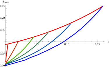
Figure 1: Thermal entropy $S_{therm}$ as a function of the temperature $T$. The upper (red) curve is for the unbroken phase (Einstein black hole). The lower (light red, orange, light green, green, blue-green and blue) curves are for hairy black holes with $\mu^{2}L^{2}=-2.2,-3,-3.5,-3.75,-3.9375,-4$ ($\Delta=3.34,3,2+1/\sqrt{2},2.5,2.25,2$). The critical temperatures are $T_{c}=0.0037,~{}0.020,~{}0.045,~{}0.070,0.106,1/2\pi$. Note the lower right (blue) curve is for the scalar at the AdS₅ BF bound, for which the critical temperature is that of the massless black hole.

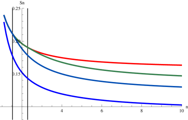
Figure 2: Rényi entropy as a function of $n$ for $\mu^{2}L^{2}=-1,-4,-3.75$ and $-3.9375$. The phase transition is at $n_{crit}\simeq 2.28$ for $\mu^{2}L^{2}=-3.75$ and $1.52$ for $\mu^{2}L^{2}=-3.9375$.

The spectral function $\bar{d}_{i}$ and $d(\lambda)$ in (18) can be obtained from the inverse Laplace transformation

$$\exp\left((1-n)S_{n}\right)=\sum_{i}\bar{d}_{i}\lambda_{i}^{n}+\int_{0}^{\lambda_{1}}d\lambda d(\lambda)\lambda^{n}.$$ (44)

We can now use our numerical results to plot the spectral density $d(\lambda)$ (including the discrete part $\bar{d}_{i}$ in $d(\lambda)$ by allowing a delta function). We will focus on the two simplest cases: $\mu^{2}L^{2}=-1$ and $\mu^{2}L^{2}=-4$, for which the critical temperatures are $T_{c}=0$ and $T_{c}=T_{0}=1/2\pi L$.

We first note that, since Renyi entropies are UV divergent, the eigenvalues are exponentially suppressed with the cutoff. For example, as explained in [13], the eigenvalue $\lambda_{1}$ scales as

$$\lambda_{1}\sim e^{-\text{const.}\times C_{T}\times\mathcal{A}/\epsilon^{d-2}}$$ (45)

where $\mathcal{A}$ and $\epsilon$ are respectively the area of the entangling surface and the UV cutoff. Here $C_{T}$ is related to the 2-point function of the stress tensor and counts the degrees of freedom of the theory, which is typically taken to be large for gravity to be classical in the bulk. For even dimensional CFTs, it is related to the A-type trace anomaly. In the bulk gravity calculation, $C_{T}$ is set by the AdS radius in Planck units ($C_{T}\sim(L/\ell_{p})^{d-1}$) and the UV divergence becomes the volume divergence of the hyperboloid. We may therefore introduce a UV regulator by taking the volume of the hyperboloid to be finite.

We can now go ahead and compute the spectral densities (44) explicitly. To exhibit a simple numerical answer, we will set $V_{{\mathbb{H}}_{d-1}}=L=G_{N}=1$. Performing an inverse Laplace transform numerically is a bit tricky, so we expand the left hand side of (44) in the large $n$ limit as

$$\exp\left((1-n)S_{n}\right)=\exp((s_{0}-s_{1})-s_{0}n)\left(1+{g_{1}\over n}+{g_{2}\over n^{2}}+{g_{3}\over n^{3}}+\cdots\right).$$ (46)

where $S_{n}=\sum_{i=0}^{\infty}s_{i}n^{-i}$ and the $g_{i}$ are functions of the $s_{i}$. The inverse Laplace transformation of the first term gives a delta function and the rest of the terms include the Heaviside step function and continuous functions. The constant $s_{0}$ determines both the location of the delta function and the Heaviside step function. The result is

$$d(\lambda)={\exp(s_{0}-s_{1})\over\lambda}(l_{0}\delta(\lambda-\lambda_{1})+\Theta(\lambda-\lambda_{1})\sum_{n=0}l_{n+1}(-\log\lambda)^{n})$$ (47)

where $l_{i}$ is a function of $s_{i}$. Note that $-\log\lambda$ is the eigenvalue of the entanglement hamiltonian $H_{E}$ (7). The numerical result for the spectral density is plotted in Fig.3. Of course, the Rényi entropies are UV-divergent but we are calculating the constant in front of the divergent piece. Similar arguments can be found in section 5 of [13].

It is worth noting that these results for the spectral density are consistent with those found by Calabrese and Lefevre [7]. In two dimensional conformal theory, the $n$ dependence of the Rényi entropy is

$$S_{n}\propto\left(1+{1\over n}\right).$$ (48)

This is determined by the conformal dimension of the twist operators. By taking the inverse Laplace transformation, Calabrese and Lefevre obtained a universal scaling behaviour for the entanglement spectrum. The structure of the spectrum, the delta function at the largest eigenvalue and the Heaviside step function, depends only on the asymptotic behaviour of the Rényi entropy at large $n$. We have found a very similar structure for our 4d CFTs.

For a general mass, it is technically difficult to perform the inverse Laplace transformation. However, from the asymptotic behaviour of the Rényi entropy, we can see that the spectral function has only one delta function which sits between $\lambda^{E}_{1}$ and $\lambda_{1}^{ES}$. Fig. 5 shows the relation between the maximum eigenvalue of $H_{E}$ and $\Delta$. Note that as we increase the dimension of the conformal operator $\Delta$, the maximum eigenvalue $\lambda_{1}$ of the entanglement spectrum monotonically decreases, i.e.

$${dS_{\infty}\over d\Delta}\geq 0$$ (49)

This suggests that the ground state of a CFT with smaller lowest dimension operator is closer to a pure state. In other words, the ground state of a theory with a large gap is more mixed than one with a small gap. This result is obtained using black hole thermodynamics, so is likely to be generic for large $N$ theories. It would be interesting to investigate the generality of this inequality, and the analytic relation between $S_{\infty}$ and $\Delta$.

Figure 3: The spectral function $d(\lambda)$ for the cases $\mu^{2}L^{2}=-1$, where the black hole is always Einstein, and $\mu^{2}L^{2}=-4$, where the black hole always has scalar hair. There are delta functions at the lowest eigenvalues, $\lambda^{E}_{1}=0.855$ for the Einstein (red line) and $\lambda^{ES}_{1}=0.911$ for the Einstein-scalar (blue line). For the pure Einstein case and with $V_{H}=G_{N}=L=1$, we obtain the same result as [13].

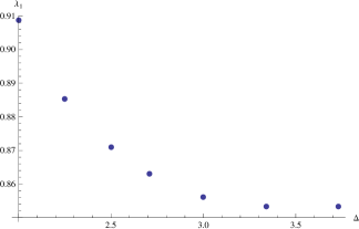
Figure 4: Lowest eigenvalue of $\rho$ as a function of conformal dimension.

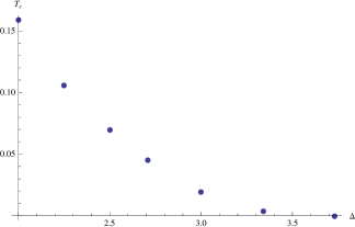
Figure 5: Critical temperature as a function of conformal dimension.

5 Instability for the Normalizable Mode

We now turn our attention to the more physical case of the mode which is normalizable on the hyperboloid. In this case the condensation of the mode will break the hyperbolic symmetries, so the construction of hairy black holes at the non-linear level is considerably more difficult. We will simply perform the linearized analysis, which is sufficient to demonstrate that an instability exists and that the Rényi entropies will undergo a phase transition. We leave the construction of hairy black hole solutions to future work.

In $d=4$, the wave equation for a scalar of mass $\mu$ is

$$\left(-\frac{\omega^{2}}{f(r)}-\frac{\lambda}{r^{2}}-\mu^{2}\right)\phi(r)+\left(f^{\prime}(r)+3\frac{f(r)}{r}\right)\phi^{\prime}(r)+f(r)\phi^{\prime\prime}(r)=0$$ (50)

where we considered the following ansatz for the field:

$$\Phi(t,r,\sigma_{i})=e^{\omega t}\phi(r)Y(\sigma_{i}),~{}~{}~{}\nabla^{2}_{\mathbb{H}_{3}}Y(\sigma_{i})=-\lambda Y(\sigma_{i}).$$ (51)

The black hole will be unstable if (50) has a solution with $\omega$ real and positive with the field satisfying specified boundary conditions at infinity and the horizon. We can put the wave equation in Schrodinger form by letting $\psi(r)=r^{(d-1)/2}\phi(r)$, so

$$\left(-\left(f(r)\frac{d}{dr}\right)^{2}+V(r)\right)\psi(r)=-\omega^{2}\psi(r)$$ (52)

with

$$V(r)=\frac{f(r)}{r^{2}}\left(\lambda+f^{\prime}(r)\frac{d-1}{2}r+f(r)\frac{(d-1)(d-3)}{4}+\mu^{2}r^{2}\right)$$ (53)

In tortoise coordinates ($dr_{*}=dr/f(r)$), this is the problem of determining whether the potential $V(r_{*})$ has a negative energy bound state. We impose the following boundary conditions

$$\psi(r_{+})=0\ \ \ \ \ \ \ \ \psi^{\prime}(r_{+})=1\ \ \ \ \ \ \ \ \ \psi(r)|_{r\to\infty}\to\frac{1}{r^{\Delta-(d-1)/2}}~{}.$$ (54)

Note that we consider here both Dirichlet and Neumann boundary conditions.

We can solve (52) numerically using a standard shooting method from the horizon. We find that, for every mass in the range

$$-\frac{d^{2}}{4}\leq\mu^{2}L^{2}_{AdS_{d+1}}\leq-\frac{d(d-1)}{4}$$ (55)

there is a temperature $T>0$ for which the Einstein black hole is unstable to the development of scalar hair. We have checked this in four and five dimensions. We plot the curve of marginal stability in Figs. 7 and 7 for four and five dimensions. Every configuration in the zone above the curves is unstable. We conclude that Rényi entropies will undergo a phase transition at values of the Rényi parameters $n_{c}$ which depend on the dimension of the lowest nontrivial operator.

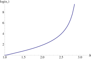
Figure 6: Log of the critical Rényi parameter for instability as a function of conformal dimension in $AdS_{5}/CFT_{4}$. As $\Delta$ approaches $3$ the instability disappears.

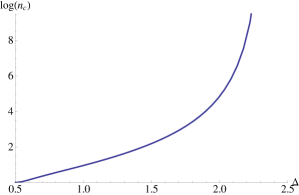
Figure 7: Log of the critical Rényi parameter for instability as a function of conformal dimension in $AdS_{4}/CFT_{3}$. The instability disappears as $\Delta\to{3+\sqrt{3}\over 2}\approx 2.37$.

These results have one important feature which distinguishes them from the instabilities considered in the previous section. They take place at $much$ lower temperatures (i.e. larger values of $n$). It turns out that, for scalars which are non-constant on the hyperboloid, the $AdS_{2}\times{\mathbb{H}}_{d-1}$ instability becomes relevant only very close to extremality. A similar phenomenon was noted in [14] for a different class of black holes. This suggests that it is primarily the lowest eigenvalues of the entanglement spectrum which are effected by the scalar field instability.

6 Acknowledgements

We thank Jaume Gomis, Nabil Iqbal, Kristan Jensen, Max Metlits, Rob Myers, Harvey Reall, Subir Sachdev, Jorge Santos, Stephen Shenker, and Tadashi Takayanagi for helpful discussions. This research was supported by the National Science and Engineering Research Council of Canada. SM thanks University of British Columbia, University of Victoria, Kavli Institute for the Physics and Mathematics of the Universe (Kavli IPMU), Kyoto University and the Perimeter Institute for theoretical physics for hospitality.

References

- [1] P. Calabrese and J. L. Cardy, “Entanglement entropy and quantum field theory,” J. Stat. Mech. 0406, P06002 (2004) [hep-th/0405152]; P. Calabrese and J. L. Cardy, “Entanglement entropy and conformal field theory” J. Phys. A42: 504005 (2009) [arXiv:0905.4013].
- [2] S. Ryu and T. Takayanagi, “Holographic derivation of entanglement entropy from AdS/CFT,” Phys. Rev. Lett. 96, 181602 (2006) [hep-th/0603001]; “Aspects of Holographic Entanglement Entropy,” JHEP 0608, 045 (2006) [hep-th/0605073]; T. Nishioka, S. Ryu and T. Takayanagi, “Holographic Entanglement Entropy: An Overview,” J. Phys. A 42, 504008 (2009) [arXiv:0905.0932 [hep-th]].
- [3] M. Levin and X. G. Wen, “Detecting topological order in a ground state wave function,” Phys. Rev. Lett., 96, 110405 (2006)[arXiv:cond-mat/0510613]; A. Kitaev and J. Preskill, “Topological entanglement entropy,” Phys. Rev. Lett. 96, 110404 (2006) [hep-th/0510092].
- [4] H. Li and F. D. M. Haldane, “Entanglement Spectrum as a Generalization of Entanglement Entropy: Identification of Topological Order in Non-Abelian Fractional Quantum Hall Effect States” Phys. Rev. Lett. 101, 010504 (2008) [arXiv:0805.0332]
- [5] A. Rényi, “On measures of information and entropy,” Procedings of the fourth Berkeley Symposium on Mathematics, Statistics and Probability 1960, 1, 547 (1961)
- [6] K. Zyczkowski, “Renyi extrapolation of Shannon entropy,” Open Syst. Inf. Dyn. 10, 297 (2003) [arXiv:quant-ph/0305062]; M.B. Hastings, I. Gonzalez, A.B. Kallin, and R.G. Melko, “Measuring Renyi Entanglement Entropy with Quantum Monte Carlo,” Phys. Rev. Lett 104, 157201 (2001) [arXiv:1001.2335]
- [7] P. Calabrese and A. Lefevre, “Entanglement spectrum in one-dimensional systems” Phys. Rev. A 78, 032329 (2008)
- [8] J.M. Stephan, G. Misguich, and V.Pasquier, “Phase transition in the Rényi-Shannon entropy of Luttinger liquids” Phys.Rev.B 84, 195128 (2011) [arXiv:1104.2544]
- [9] I. R. Klebanov, S. S. Pufu, S. Sachdev and B. R. Safdi, “Renyi Entropies for Free Field Theories,” JHEP 1204, 074 (2012) [arXiv:1111.6290 [hep-th]].
- [10] M. Headrick, “Entanglement Renyi entropies in holographic theories,” Phys. Rev. D 82, 126010 (2010) [arXiv:1006.0047 [hep-th]]; T. Faulkner, “The Entanglement Renyi Entropies of Disjoint Intervals in AdS/CFT,” arXiv:1303.7221 [hep-th]; A. Lewkowycz and J. Maldacena, “Generalized gravitational entropy,” arXiv:1304.4926 [hep-th].
- [11] D. V. Fursaev, “Entanglement Renyi Entropies in Conformal Field Theories and Holography,” JHEP 1205, 080 (2012) [arXiv:1201.1702 [hep-th]].
- [12] H. Casini, M. Huerta and R. C. Myers, “Towards a derivation of holographic entanglement entropy,” JHEP 1105, 036 (2011) [arXiv:1102.0440 [hep-th]].
- [13] L. -Y. Hung, R. C. Myers, M. Smolkin and A. Yale, “Holographic Calculations of Rényi Entropy,” JHEP 1112, 047 (2011) [arXiv:1110.1084 [hep-th]]; D. A. Galante and R. C. Myers, “Holographic Rényi Entropies at Finite Coupling,” arXiv:1305.7191 [hep-th].
- [14] O. J. C. Dias, R. Monteiro, H. S. Reall and J. E. Santos, “A Scalar field condensation instability of rotating anti-de Sitter black holes,” JHEP 1011, 036 (2010) [arXiv:1007.3745 [hep-th]].
- [15] S. A. Hartnoll, C. P. Herzog and G. T. Horowitz, “Building a Holographic Superconductor,” Phys. Rev. Lett. 101, 031601 (2008) [arXiv:0803.3295 [hep-th]]; “Holographic Superconductors,” JHEP 0812, 015 (2008) [arXiv:0810.1563 [hep-th]]; S. S. Gubser, “Colorful horizons with charge in anti-de Sitter space,” Phys. Rev. Lett. 101, 191601 (2008) [arXiv:0803.3483 [hep-th]].
- [16] M.A. Metlitski, C.A. Fuertes, and S. Sachdev “Entanglement Entropy in the O(N) model”, Phys. Rev. B 80, 115122 (2009) [arXiv:0904.4477 [cond-mat]], S. Sachdev, Private Communication.
- [17] I. Klebanov and A. Polyakov, “AdS Dual of the Critical O(N) Vector Model” [arXiv:0210114 [hep-th]],
- [18] D. N. Kabat and M. J. Strassler, “A Comment on entropy and area,” Phys. Lett. B 329, 46 (1994) [hep-th/9401125].
- [19] A. Belin, L. -Y. Hung, A. Maloney, S. Matsuura, R. C. Myers and T. Sierens, JHEP 1312, 059 (2013) [arXiv:1310.4180 [hep-th]].
- [20] A. Belin, L. Y. Hung, A. Maloney and S. Matsuura, JHEP 1501, 059 (2015) [arXiv:1407.5630 [hep-th]].
- [21] A. Belin and A. Maloney, arXiv:1412.0280 [hep-th].