Magnetically generated spin-orbit coupling for ultracold atoms

Abstract

We present a new technique for producing two and three dimensional Rashba-type spin-orbit coupling for ultra cold atoms without involving light. The method relies on a sequence of pulsed inhomogeneous magnetic fields imprinting suitable phase gradients on the atoms. For sufficiently short pulse durations, the time-averaged Hamiltonian well approximates the Rashba Hamiltonian. Higher order corrections to the energy spectrum are calculated exactly for spin-$1/2$ and perturbatively for higher spins. The pulse sequence does not modify the form of rotationally symmetric atom-atom interactions. Finally, we present a straightforward implementation of this pulse sequence on an atom-chip.

Proposals for creating Rashba type spin-orbit coupling (SOC) in cold atomic gases abound Dudarev et al. (2004); Ruseckas et al. (2005); Stanescu and Galitski (2007); Jacob et al. (2007); Juzeliūnas et al. (2008); Stanescu et al. (2008); Vaishnav and Clark (2008); Juzeliūnas et al. (2010); Campbell et al. (2011); Dalibard et al. (2011); Zhai (2012); Xu and You (2012); Anderson et al. (2012); Galitski and Spielman (2013). All of these schemes rely (at least partially Xu and You (2012)) on the coupling of atoms to laser beams. Unfortunately, the atom-light interaction is associated with spontaneous emission, leading to heating or loss. To date, only the experimentally most simple case – an equal mixture of Rashba and Dresselhaus SOC – has been realized in the lab Lin et al. (2011); Zhang et al. (2012); Wang et al. (2012); Cheuk et al. (2012). Implementation of Rashba SOC would allow for the study of rich ground state physics proposed in systems of many-body fermions Liu et al. (2009); Vyasanakere and Shenoy (2011); Vyasanakere et al. (2011); Jiang et al. (2011); Hu et al. (2011); Liu et al. (2012); Chen et al. (2012); He and Huang (2012); Cui et al. (2012); Zheng et al. (2013); Mundo et al. (2013) and bosons Stanescu et al. (2008); Sinha et al. (2011); Radic et al. (2011); Wu et al. (2011); Hu et al. (2012); Su et al. (2012); Kawakami et al. (2012); Ruokokoski et al. (2012); Xu et al. (2012); Sedrakyan et al. (2012); Song et al. (2012), of which many properties have no condensed matter analogue.

Rashba SOC can be intuitively understood as a momentum-dependent magnetic field that is symmetric under simultaneous spin and momentum rotations. Generically, realizing such behavior requires terms in the atomic Hamiltonian which link spin to momentum. Laser beams using two-photon Raman transitions are an obvious choice for implementing such coupling, as they induce transitions between two internal states while simultaneously imparting momentum.

Here we demonstrate that Rashba or Dresselhaus SOC can be created in cold atoms without any optical fields by imprinting phase gradients in different directions using a properly chosen pulse sequence of inhomogeneous magnetic fields. This linearly varying magnetic field provides a uniform spin-dependent force, imparting a desired momentum. When the direction of the magnetic field and the gradient of its magnitude are perpendicular to each other, the form of the momentum boost represents a position dependent rotation of the atomic spin. This suggests pulsed magnetic field gradients have the necessary features to produce Rashba or Dresselhaus SOCs.

The current scheme can be realized in a straightforward manner on state-of-the-art atom chips Trinker et al. (2008); Goldman et al. (2010)with SOC strengths comparable with those in optical implementations. In contrast, the optical schemes rely on using many laser beams that couple internal atomic states in a complex way. The proposal is applicable to any atomic species containing an arbitrary non-zero spin and does not alter the form of $SU(2)$ invariant atom-atom interactions Ohmi and Machida (1998); Ho (1998); Kawaguchi and Ueda (2012). Our proposal allows for study of spin-1 and spin-2 SOC bosons, where the symmetry of the atom-atom interactions strongly affects the symmetry of the many-body ground state Su et al. (2012); Ruokokoski et al. (2012); Xu et al. (2012); Song et al. (2012). In optical setups, Dalibard et al. (2011) the adiabatic elimination of a number of atomic states makes the atom-atom interaction position-dependent and not $SU(2)$ invariant.

Time averaged descriptions of periodically driven systems can often acquire gauge fields, the most simple example of which is the transformation into a rotating frame Franzosi et al. (2004); Fetter (2009); Cooper (2008). One can also generate artificial magnetic fields by combining lattice and time-dependent quadrupolar potentials Sørensen et al. (2005), or by shaking Graham et al. (1992); Madison et al. (1998); Eckardt et al. (2005, 2010); Hemmerich (2010); Kolovsky (2011); Struck et al. (2012); Arimondo et al. (2012) or stirring Kitagawa et al. (2010) optical lattices. Here we focus on a different scenario where a time dependent magnetic field yields SOC (rather than an Abelian magnetic flux) for atoms in the continuum (rather than on a lattice). Unlike the case for conventional magnetic trapping where the atomic spin adiabatically follows the local magnetic field Migdall et al. (1985), here the field pulses time average to zero, provide no trapping potential, and lead to dynamic spin evolution.

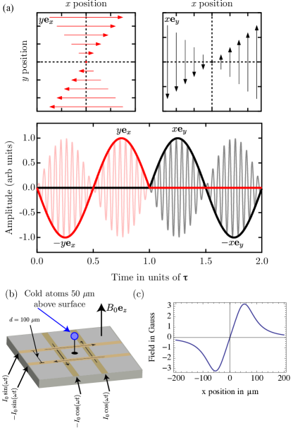
Figure 1: Proposed atom chip implementation of 2D Rashba SOC using pulsed magnetic fields. (a) One full pulse of period $2\tau$. For $0\leq t<\tau$ an effective coupling vector $\boldsymbol{\Omega}_{x}=-\beta\left(t\right)k_{{\rm eff}}y{\mathbf{e}}_{x}$ (red) writes a spin-dependent phase gradient along $y$ in the quantization basis of $F_{x}$. In the second half of the pulse, $\tau\leq t<2\tau$, the coupling vector $\boldsymbol{\Omega}_{y}=\beta\left(t-\tau\right)k_{{\rm eff}}x{\mathbf{e}}_{y}$ (black) writes a phase gradient along $x$ in the quantization basis of $F_{y}$. (b) The cloud of atoms sits $50\mu{\rm m}$ above the surface of an atom chip. A strong bias field $B_{0}{\mathbf{e}}_{z}$ sets a quantization axis. Two sets of microwires wires parallel to ${\mathbf{e}}_{x}$ and ${\mathbf{e}}_{y}$ are spaced $50\mu{\rm m}$ from the center of the cloud in the ${\mathbf{e}}_{x}-{\mathbf{e}}_{y}$ plane carry an amplitude modulated rf current. (c) The current configuration produces a magnetic field gradient that is linear near the center of the atom-chip.

General Formulation:

We focus on the atoms in a spin-$f$ hyperfine ground state manifold characterized by the spin vector $\mathbf{F}$ with components obeying the commutation relations $[F_{i},F_{j}]=i\hbar\epsilon_{ijk}F_{k}$. The interaction of the atom and the magnetic field $\mathbf{B}\equiv\mathbf{B}(\mathbf{r},t)$ is given by the Hamiltonian

$$H_{\mathbf{B}}(\mathbf{r},t)=\boldsymbol{\Omega}(\mathbf{r},t)\cdot\mathbf{F}\,,$$ (1)

with $\boldsymbol{\Omega}\left(\mathbf{r},t\right)=g_{F}\mu_{B}\mathbf{B}$, where $\mu_{B}$ is the Bohr magneton and $g_{F}$ is the the Landé g-factor. The Schrödinger equation describing the combined internal and center of mass evolution of the atom is

$$i\hbar\partial_{t}\left|\psi\right\rangle=\left[H_{0}+V+H_{\mathbf{B}}(\mathbf{r},t)\right]\left|\psi\right\rangle,$$ (2)

with $H_{0}=\mathbf{p}^{2}/2m$, where $\mathbf{r}$ and $\mathbf{p}$ are, respectively, the atomic center of mass coordinate and momentum operators obeying $\left[r_{i},p_{j}\right]=i\hbar\delta_{ij}$. In what follows, we will neglect the state-independent trapping potential $V$.

1D SOC:

We first show a properly chosen pulsed magnetic field gradient can give rise to a 1D SOC. In the first stage, $0\leq t<\tau$, an effective coupling vector $\boldsymbol{\Omega}_{x}=-\beta\left(t\right)k_{{\rm eff}}y{\mathbf{e}}_{x}$ writes a spin-dependent phase gradient along ${\mathbf{e}}_{y}$ (where $\mathbf{e}_{xyz}$ denote the Cartesian unit vectors) in the quantization basis of $F_{x}$, where the wavevector $k_{{\rm eff}}$ characterizes the strength of the magnetic field gradient, and $\beta\left(t\right)$ defines its temporal shape. While a magnetic field $\mathbf{B}\sim y{\mathbf{e}}_{x}$, cannot exist in region of zero electric currents, in the experimental section we will show how to produce a coupling Hamiltonian Eq. (1) corresponding to $\boldsymbol{\Omega}_{x}$ using a strong bias magnetic field along $\mathbf{e}_{z}$, and a fast oscillating magnetic field in the ${\mathbf{e}}_{x}-{\mathbf{e}}_{z}$ plane, as shown in Fig. 1.

To elucidate the main idea, suppose that at times $t=0$ and $t=\tau$, $\mathbf{B}$ is pulsed for a short enough duration that the atoms hardly move, i.e., $\beta\left(t\right)=\delta\left(t-\epsilon\right)-\delta\left(t-\tau+\epsilon\right)$ with $\epsilon\rightarrow 0$. The pulse at $t=0$ rotates the spin about ${\mathbf{e}}_{x}$ according to the operator $R_{x}=\exp\left[ik_{{\rm eff}}yF_{x}/\hbar\right]$. The particle then evolves freely for a time $\tau$ before a second pulse “undoes” the rotation, described by $R_{x}^{\dagger}$. The total evolution of the particle after both pulses is described by

$$U_{x}\left(\tau\right)=R_{x}e^{-\frac{iH_{0}\tau}{\hbar}}R_{x}^{\dagger}=\exp\left[-i\frac{\left(\mathbf{p}-k_{{\rm eff}}F_{x}{\mathbf{e}}_{y}\right)^{2}}{2m\hbar}\tau\right],\,$$ (3)

representing the evolution for a particle with SOC along ${\mathbf{e}}_{y}$.

The analysis leading Eq. (3) can be readily extended to any pulse of finite width and zero average $\int_{0}^{\tau}\beta\left(t\right)dt=0$. This coupling can be eliminated from Eq. (2) by the unitary transformation $R_{x}(t)=\exp\left[iF_{x}k_{{\rm eff}}y\int_{0}^{t}\beta\left(t^{\prime}\right)\,dt^{\prime}/\hbar\right]$ which also changes the momentum $\mathbf{p}$ to $\mathbf{p}^{\prime}=\mathbf{p}-k_{{\rm eff}}F_{x}{\mathbf{e}}_{y}\int_{0}^{t}\beta\left(t^{\prime}\right)\,dt^{\prime}$ in the transformed Hamiltonian $\tilde{H}_{0}\left(t\right)=R_{x}\left(t\right)H_{0}R_{x}^{\dagger}\left(t\right)=\mathbf{p}^{\prime 2}/2m$. The latter $\tilde{H}_{0}\left(t\right)$ commutes with itself at different times. Thus, using $R_{1}\left(\tau\right)=1\!\!1$, where $1\!\!1$ is the identity operator in spin space, one can exactly calculate the time evolution operator $U_{x}\left(\tau\right)=\exp\left[-i\int_{0}^{\tau}\tilde{H}_{0}\left(t\right)\,dt/\hbar\right]$ after one pulse, giving:

$$U_{x}\left(\tau\right) = \exp\left[-\frac{i\tau}{\hbar}\left(\frac{\left(\mathbf{p}-c_{1}k_{{\rm eff}}F_{x}{\mathbf{e}}_{y}\right)^{2}}{2m}+s\frac{k_{{\rm eff}}^{2}}{2m}F_{x}^{2}\right)\right]\,$$ (4)

where $s=c_{2}-c_{1}^{2},$ with $c_{n}=\tau^{-1}\int_{0}^{\tau}\mathrm{d}t^{\prime}\left[\int_{0}^{t^{\prime}}\beta\left(t^{\prime\prime}\right)\mathrm{d}t^{\prime\prime}\right]^{n}$. For two delta pulses, $\beta\left(t\right)=\delta\left(t-\epsilon\right)-\delta\left(t-\tau+\epsilon\right)$, we have $c_{1}=1$ and $s=0$, so one arrives at Eq. (3). For a smoothly alternating coupling, $\beta\left(t\right)=\frac{2\pi}{\tau}\sin\left(2\pi\frac{t}{\tau}+\varphi\right)$, where $\varphi$ sets the origin of time, one has that $c_{1}=\cos\varphi$ and $s=1/2$. If the pulse is repeated many times, the choice of $\varphi$ cannot matter. Indeed, the vector potential $c_{1}k_{{\rm eff}}F_{x}{\mathbf{e}}_{y}$ in Eq. (4) can be eliminated by a gauge transformation. In the next section, a second pulse at times $\tau\leq t<2\tau$ breaks time translation symmetry. The vector potential then cannot be gauged away, and only signals $\beta_{a}\left(t\right)=\left(\beta\left(t\right)-\beta\left(\tau-t\right)\right)/2$, antisymmetric over one period, will contribute to $c_{1}$, with a maximum of $c_{1}=1$ for $\varphi=0$. Since the magnetic pulse strength depends only on the product $\beta\left(t\right)k_{{\rm eff}}$, we will henceforth set $c_{1}=1$, which can always be done through a re-definition of $k_{{\rm eff}}$.

2D SOC:

To add SOC in another direction, at $\tau\leq t<2\tau$, we introduce a second stage during which $\boldsymbol{\Omega}\equiv\boldsymbol{\Omega}_{y}=\beta\left(t-\tau\right)k_{{\rm eff}}x{\mathbf{e}}_{y}$ with the same temporal behavior as the first stage. The unitary operator $U_{y}(\tau)$, evolving the system from $t=\tau$ to $t=2\tau$, has the form of Eq. (4) with ${\mathbf{e}}_{y}\rightarrow-{\mathbf{e}}_{x}$ and $F_{x}\rightarrow F_{y}$.

These two stages together, with $U_{xy}\equiv U_{y}U_{x}$ describe a single full cycle of our repeating pulse sequence. Thus the Hamiltonian is time-periodic with period $2\tau$. For a sufficiently short period, the combined evolution operator $U_{xy}$ can be well approximated using the Baker-Campbell-Hausdorff formula, up to first order in $\tau$, giving $U_{xy}\approx\exp\left[-iH_{2D}2\tau/\hbar\right]$, where

$$H_{2D}=\frac{p^{2}}{2m}-k_{{\rm eff}}\frac{p_{y}F_{x}-p_{x}F_{y}}{2m}+c_{2}k_{{\rm eff}}^{2}\frac{F_{x}^{2}+F_{y}^{2}}{4m}$$ (5)

is the effective Hamiltonian describing the evolution of the system under our repeated pulse sequence, observed at integer multiples of $2\tau$.

For the spin-$1/2$ case with $\mathbf{F}=\hbar\boldsymbol{\sigma}/2$, Eq. (5) reduces to the Rashba Hamiltonian,

$$H_{2D}=H_{R}=\frac{\mathbf{p}^{2}}{2m}-v\boldsymbol{\sigma}\cdot\left({\mathbf{e}}_{z}\times\mathbf{p}\right)\,,\quad\textrm{with}\quad v=\frac{\hbar k_{{\rm eff}}}{4m}\,,$$ (6)

where an overall energy offset has been omitted. For higher spins ($f>1/2$) the last term in Eq. (5) is proportional to $\hbar^{2}f\left(f+1\right)1\!\!1-F_{z}^{2}$, introducing an effective quadratic Zeeman (QZ) shift. Since $c_{2}>0$, using the two-dimensional setup it is thus impossible to completely eliminate the QZ term in Eq. (5) for $f\neq 1/2$, and produce the Rashba Hamiltonian in Eq. (6) with $\boldsymbol{\sigma}$ replaced by $2\mathbf{F}/\hbar$. The QZ term preserves the conserved quantum number $J_{z}=L_{z}+F_{z}$, where $L_{z}=xp_{y}-yp_{x}$, so it is unlikely to significantly affect the ground state phases explored in systems with higher spin Rashba SOC Su et al. (2012); Xu et al. (2012); Ruokokoski et al. (2012).

We validated this approach by numerically simulating the trapped, weakly interacting Gross-Pitaevskii equation and non-interacting Schrödinger equation. We applied the periodic pulse sequence described above to the ground state without SOC, and slowly ramped on $k_{{\rm eff}}$. When measured at full periods, the system was similar to the ground states found in Ref. Sinha et al. (2011); Hu et al. (2012). We also used imaginary time propagation to find the true Rashba ground state, followed by the pulsed Rashba SOC described above, where $k_{{\rm eff}}$ was matched to the minimum of the Rashba ring. If viewed at complete periods, the system did not significantly deviate from the many-body ground state. These numerical tests suggest that the proposed SOC system well approximates Rashba SOC.

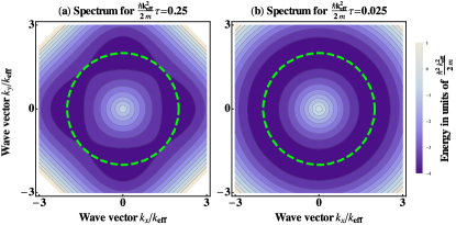
Figure 2: The lower band of the the exact time-averaged Hamiltonian of a spin-$1/2$ particle under the influence of the pulsed magnetic field scheme described in the main text. (a) For long evolution times, $\hbar k_{{\rm eff}}^{2}\tau/2m=0.25$, the spectrum has a Bloch structure of periodicity $4\pi m/k_{{\rm eff}}\tau$ superposed on the $\mathbf{p}^{2}/2m$ dispersion of a free particle. (b) Short evolution times, $\hbar k_{{\rm eff}}^{2}\tau/2m=.025$ well approximate the Rashba ring. The green dashed line represents the minimum energy “Rashba ring” of $H_{2D}$ in Eq. (6).

3D Spin-orbit coupling

Pulsed magnetic fields can provide not only the conventional two-dimensional Rashba or Dresselhaus coupling, but also three-dimensional (3D) SOC which is not encountered for electrons in condensed matter structures. By adding an additional pulse oriented along the ${\mathbf{e}}_{z}$ direction, all three spin matrices $\left\{F_{x},F_{y},F_{z}\right\}$ can be coupled to momentum. For instance, using three magnetic coupling stages $\boldsymbol{\Omega}\equiv\boldsymbol{\Omega}_{x}=-\beta\left(t\right)k_{{\rm eff}}x{\mathbf{e}}_{y}$ for $0\leq t<\tau$, $\boldsymbol{\Omega}\equiv\boldsymbol{\Omega}_{y}=-\beta\left(t-\tau\right)k_{{\rm eff}}y{\mathbf{e}}_{z}$ for $\tau\leq t<2\tau$ and $\boldsymbol{\Omega}\equiv\boldsymbol{\Omega}_{z}=-\beta\left(t-2\tau\right)k_{{\rm eff}}z{\mathbf{e}}_{x}$ for $2\tau\leq t<3\tau$ and using a procedure analogous to the one presented above, one can simulate a spin-orbit coupling

$$H_{3D}=\frac{\mathbf{p}^{2}}{2m}-v\frac{2}{\hbar}\left(p_{x}F_{y}+p_{y}F_{z}+p_{z}F_{x}\right)\,,$$ (7)

with $v=\hbar k_{{\rm eff}}/6m$, describing the 3D SOC of the Rashba type. This scheme has an additional advantage over 2D Rashba spin-orbit coupling in that the quadratic term featured in Eq. (5) is proportional to $\mathbf{F}^{2}=\hbar^{2}f\left(f+1\right)1\!\!1$, which is a constant and thus has been omitted in Eq. (7). Therefore, the 3D setup simulates a pure spin-orbit coupling without a quadratic Zeeman term for arbitrary spin systems. The present proposal allows for creating 3D SOC in a more simple manner without any use of optical fields. Previous proposals to produce a 3D SOC involve complex optical transitions between four or more internal atomic states Anderson et al. (2012); Li et al. (2012).

Corrections to the 2D Single particle spectrum:

In the derivation of Eq. (5), the product $U_{y}U_{x}$ was expanded to lowest order in the short time $\tau$. In practice, a finite pulse time $\tau$ will result in deviations from the ideal SOC form. For a spin-$1/2$ system, the effective Hamiltonian for the 2D system can be calculated exactly using $U_{y}U_{x}=\exp\left(-i\mathbf{p}^{2}\tau/m\hbar\right)S_{\left(yx\right)}^{\dagger}S_{\left(xy\right)}$, where $S_{\left(uv\right)}=\exp\left(i\gamma_{u}\sigma_{v}\right)=\cos\gamma_{u}+i\sigma_{v}\sin\gamma_{u}$ is a rotation matrix and $\gamma_{u}=k_{{\rm eff}}p_{u}\tau/2m$ is the corresponding momentum-dependent angle. The product of two rotations is itself a rotation $S_{\left(yx\right)}^{\dagger}S_{\left(xy\right)}=\exp\left(i\gamma\hat{\mathbf{n}}\cdot\boldsymbol{\sigma}\right)$ around an axis $\hat{\mathbf{n}}$ by an angle $\gamma\equiv\gamma\left(\mathbf{p}\right)$, implicitly defined by $\cos\gamma=\cos\gamma_{x}\cos\gamma_{y}$ and $\hat{\mathbf{n}}\sin\gamma={\mathbf{e}}_{x}\cos\gamma_{x}\sin\gamma_{y}-{\mathbf{e}}_{y}\sin\gamma_{x}\cos\gamma_{y}-{\mathbf{e}}_{z}\sin\gamma_{x}\sin\gamma_{y}$. The exact time-averaged Hamiltonian is then given by $H_{2D}^{\left(\mathrm{exact}\right)}=\frac{\mathbf{p}^{2}}{2m}-\frac{\hbar}{2\tau}\gamma\hat{\mathbf{n}}\cdot\boldsymbol{\sigma}+{\rm const}$.

This allows for a straightforward calculation of the deviations of the time-averaged eigenstates from the ideal Rashba form. The lower band has energy given by $E\left(\mathbf{p}\right)=\frac{\mathbf{p}^{2}}{2m}-\frac{\hbar}{2\tau}\gamma\left(\mathbf{p}\right)$. We plot this spectrum as a function of momentum in Fig. (2). For long pulses, $\tau\gg 2m/\hbar k_{{\rm eff}}^{2}$, the structure resembles a periodic band structure with an overall $\mathbf{p}^{2}/2m$ envelope. The periodicity of $\gamma\left(\mathbf{p}\right)$ in momentum space is given by $\hbar k_{p}=4\pi m/k_{{\rm eff}}\tau$. In the opposite limit where $\tau\ll 2m/\hbar k_{{\rm eff}}^{2}$, the periodicity of $\gamma\left(\mathbf{p}\right)$ becomes much longer than the characteristic momentum $\hbar k_{{\rm eff}}$ which sets the momentum scale of the Rashba spin-orbit term. Thus, for sufficiently short pulses and sufficiently small momentum, the spectrum well approximates Rashba spin-orbit coupling.

For spin-$f>1/2$ particles, the QZ terms $F_{x}^{2}$ and $F_{y}^{2}$ featured in $U_{x}$ and $U_{y}$ do not allow for an exact solution. For short pulses, $\hbar k_{{\rm eff}}^{2}\tau/2m\ll 1$, higher order corrections to the average Hamiltonian can be found perturbatively. The first order correction $\delta\bar{H}^{\left(1\right)}$ is

$$\delta\bar{H}^{\left(1\right)} = \frac{\tau}{4}\left(\frac{k_{{\rm eff}}^{2}}{2m}\right)^{2}\left(-4\frac{p_{x}p_{y}}{k_{{\rm eff}}^{2}}F_{z}-2c_{2}\frac{p_{y}}{k_{{\rm eff}}}\left\{F_{y},F_{z}\right\}\right.$$ (8)

$$\qquad\left.+2c_{2}\frac{p_{x}}{k_{{\rm eff}}}\left\{F_{x},F_{z}\right\}+c_{2}^{2}\left\{F_{x},\left\{F_{y},F_{z}\right\}\right\}\right),\,$$

where we have assumed that $p_{x}/\hbar k_{{\rm{}_{eff}}}$ and $p_{y}/\hbar k_{{\rm eff}}$ are both $\mathcal{O}\left(1\right)$. At large momenta, $|\mathbf{p}|/\hbar k_{{\rm eff}}\gg 1$, the expansion will break down. For a spin-1/2 system, the anticommutators vanish, and only the first term proportional to $p_{x}p_{y}F_{z}$ remains in Eq. (8). This term and higher order corrections can also be obtained by expanding, for small pulse durations $\tau$, the angle $\gamma\left(\mathbf{p}\right)$ featured in the exact Hamiltonian $H_{2D}^{\left(\mathrm{exact}\right)}$. For higher spin systems, the anticommutators produce corrections that cannot be expressed using only the original angular momentum algebra. In general, the $n$-th order correction will contain nested anti-commutators of the operators $F_{x}$, $F_{y}$ and $F_{z}$ of order up to $n+2$.

Interactions:

We now consider the addition of the interaction Hamiltonian $\mathcal{H}_{I}=\frac{g_{abcd}}{2}\int d\mathbf{r}\psi_{a}^{\dagger}\psi_{b}^{\dagger}\psi_{c}\psi_{d}$, where $\psi_{a}\left(\mathbf{r}\right)\left(\psi_{a}^{\dagger}\left(\mathbf{r}\right)\right)$ is a Bose or Fermi annihilation(creation) operator for a particle with spin $a$ at position $\mathbf{r}$, and $g_{abcd}$ is a spin-dependent interaction constant. The full Hamiltonian in the presence of interactions is $\mathcal{H}=\mathcal{H}_{0}+\mathcal{H}_{I}$, where $\mathcal{H}_{0}=\int d\mathbf{r}\>\psi_{a}^{\dagger}\left[H_{0}+H_{\mathbf{B}}(\mathbf{r},t)\right]_{ab}\psi_{b}$. In the absence of an external field to break rotational symmetry, interactions must be $SU(2)$ invariant, and will be unaffected by the transformation to the rotating frame which eliminated the magnetic field. It can be seen that for a sufficiently short pulse, the effective many-body Hamiltonian is given by $\mathcal{H}_{2D}=\int d\mathbf{r}\psi_{a}^{\dagger}\left(H_{2D}\right)_{ab}\psi_{b}+\mathcal{H}_{I}$. In other words, the effective spin-orbit coupling does not modify the form or symmetry of the interactions.

Experimental implementation

Quasi-dc magnetic fields $\mathbf{B}({\bf r})$ can be approximated with the series $B_{j}({\bf r})\approx B_{j}^{(0)}+B_{jk}^{(1)}r_{k}+\cdots$. Since there are no electrical currents inside the atomic cloud, the divergence and curl of $\mathbf{B}\left(\mathbf{r}\right)$ are zero. This constrains $B_{jk}^{(1)}$ to be a symmetric traceless matrix. Hence the magnetic fields used in our previous analysis, such as ${\bf B}\propto x{\mathbf{e}}_{y}$ cannot exist and are accompanied by a counter term such as $y{\mathbf{e}}_{x}$. The constraint can be lifted by applying a combination of a strong bias field $B^{(0)}{\mathbf{e}}_{z}$ and a rf field of frequency $\omega=g_{F}\mu_{{\rm B}}B^{(0)}/\hbar$, such as ${\bf B}_{x}({\bf r},t)=B^{(0)}{\mathbf{e}}_{z}+B^{(1)}\left(t\right)\cos(\omega t+\phi_{x})\left(x{\mathbf{e}}_{x}-z{\mathbf{e}}_{z}\right)$, where $B^{(1)}\left(t\right)$ is an envelope function that is slowly varying compared to $1/\omega$. The bias field and the fast temporal dependence of the rf field entering $H_{\mathbf{B}}(\mathbf{r},t)$ can be eliminated via a position-independent rotation $S=\exp\left[i\omega tF_{z}/\hbar\right]$ of the spin around ${\mathbf{e}}_{z}$ with frequency $\omega$. Terms oscillating at frequencies $\omega$ and $2\omega$ are removed through the rotating wave approximation in the transformed Hamiltonian $SH_{\mathbf{B}}(\mathbf{r},t)S^{\dagger}-i\hbar S\partial_{t}S^{\dagger}$, giving Eq. (1) with

$$\boldsymbol{\Omega}_{x}({\bf r},t) =\frac{g_{F}\mu_{B}B^{(1)}\left(t\right)}{2\hbar}x\left({\mathbf{e}}_{x}\cos\phi_{x}+{\mathbf{e}}_{y}\sin\phi_{x}\right).$$ (9)

The field $\boldsymbol{\Omega}_{x}({\bf r},t)=-\beta\left(t\right)k_{{\rm eff}}x{\mathbf{e}}_{y}$ in the first stage of the 2D setup is obtained with the phase $\phi_{x}=-\pi/2$, where $\beta\left(t\right)k_{{\rm eff}}=g_{F}\mu_{B}B^{(1)}\left(t\right)/2\hbar$. Thus the pulsed-gradient magnetic field described in the preceding sections is represented by the envelope functions which shape the rf field.

In the second stage of a two-dimensional setup the magnetic field ${\bf B}_{y}({\bf r},t)=B^{(0)}{\mathbf{e}}_{z}+B^{(1)}\left(t-\tau\right)\cos(\omega t+\phi_{y})\left(y{\mathbf{e}}_{y}-z{\mathbf{e}}_{z}\right)$ leads to

$$\boldsymbol{\Omega}_{y}({\bf r},t) =\frac{g_{F}\mu_{B}B^{(1)}\left(t-\tau\right)}{2\hbar}y\left(-{\mathbf{e}}_{x}\sin\phi_{y}+{\mathbf{e}}_{y}\cos\phi_{y}\right).$$ (10)

For $\phi_{y}=-\pi/2$ we reproduce the second stage magnetic field $\boldsymbol{\Omega}_{y}({\bf r},t)=\beta\left(t-\tau\right)k_{{\rm eff}}x{\mathbf{e}}_{y}$. Only the phase difference $\phi_{x}-\phi_{y}$ is relevant, the absolute phase reflects the choice of the origin of time.

Figure 1 shows an atom-chip implementation of the 2D SOC of the Rashba-type. A constant bias field $B^{(0)}{\mathbf{e}}_{z}$ is applied out of plane, and two pairs of microwires parallel to ${\mathbf{e}}_{x}$ and ${\mathbf{e}}_{y}$ provide the rf magnetic fields ${\bf B}_{x}({\bf r},t)$ and ${\bf B}_{y}({\bf r},t)$, respectively. By properly timing the currents in the pairs of wires, one arrives at the required effective magnetic couplings $\boldsymbol{\Omega}_{x}({\bf r},t)$ and $\boldsymbol{\Omega}_{y}({\bf r},t)$. Realistic values Trinker et al. (2008) of $B^{(0)}=20{\rm G}$, $B^{(1)}=0.06{\rm G}/\mu{\rm m}$, and $\beta\left(t\right)=\frac{2\pi}{\tau}\sin\left(2\pi\frac{t}{\tau}\right)$ with $\tau=50\mu{\rm s}$ give an estimate of $k_{{\rm eff}}\approx 1\mu{\rm m}^{-1}$, compared to optically induced SOC in Rubidium where $k_{{\rm eff}}\approx 8\mu{\rm m}^{-1}$ Lin et al. (2011); Zhang et al. (2012). The creation of a 3D SOC would be a much more challenging experimental task. In that case one not only needs to use several rf pulses with the magnetic field oriented along different planes, but also periodically alter the direction of the bias field.

Summary:

We proposed a scheme to simulate Rashba spin-orbit coupling in an arbitrary spin-$f$ gas of ultracold atoms. The scheme used pulsed magnetic field gradients along perpendicular directions to impart a spin-dependent momentum boost to the atoms. For sufficiently short evolution time, the time-averaged Hamiltonian well approximated the Rashba Hamiltonian. Higher order corrections to the energy spectrum were calculated exactly for spin-$1/2$ and perturbatively for higher spins. We then considered interactions, and found that for short pulses, the form of the interactions is not modified. Finally, we proposed an experimental implementation of such a scheme on atom-chips.

Note:

After submission of this manuscript, an article by Xu, et. al., Xu et al. (2013) appeared that also considers Rashba SOC using pulsed magnetic field gradients.

References

- Dudarev et al. (2004) A. M. Dudarev, R. B. Diener, I. Carusotto, and Q. Niu, Phys. Rev. Lett. 92, 153005 (2004).
- Ruseckas et al. (2005) J. Ruseckas, G. Juzeliunas, P. Ohberg, and M. Fleischhauer, Phys. Rev. Lett. 95, 010404 (2005).
- Stanescu and Galitski (2007) T. D. Stanescu and V. Galitski, Phys. Rev. B 75, 125307 (2007).
- Jacob et al. (2007) A. Jacob, P. Öhberg, G. Juzeliūnas, and L. Santos, Appl. Phys. B 89, 439 (2007).
- Juzeliūnas et al. (2008) G. Juzeliūnas, J. Ruseckas, M. Lindberg, L. Santos, and P. Öhberg, Phys. Rev. A 77, 011802(R) (2008).
- Stanescu et al. (2008) T. D. Stanescu, B. Anderson, and V. Galitski, Phys. Rev. A 78, 023616 (2008).
- Vaishnav and Clark (2008) J. Y. Vaishnav and C. W. Clark, Phys. Phys. Lett. 100, 153002 (2008).
- Juzeliūnas et al. (2010) G. Juzeliūnas, J. Ruseckas, and J. Dalibard, Phys. Rev. A 81, 053403 (2010).
- Campbell et al. (2011) D. L. Campbell, G. Juzeliūnas, and I. B. Spielman, Phys. Rev. A 84, 025602 (2011).
- Dalibard et al. (2011) J. Dalibard, F. Gerbier, G. Juzeliūnas, and P. Öhberg, Rev. Mod. Phys. 83, 1523 (2011).
- Zhai (2012) H. Zhai, International Journal of Modern Physics B 26, 1230001 (2012).
- Xu and You (2012) Z. F. Xu and L. You, Phys. Rev. A 85, 043605 (2012).
- Anderson et al. (2012) B. M. Anderson, G. Juzeliūnas, V. M. Galitski, and I. B. Spielman, Phys. Lett. Lett. 108, 235301 (2012).
- Galitski and Spielman (2013) V. Galitski and I. B. Spielman, Nature 494, 49 (2013).
- Lin et al. (2011) Y.-J. Lin, K. Jiménez-García, and I. B. Spielman, Nature 471, 83 (2011).
- Zhang et al. (2012) J.-Y. Zhang, S.-C. Ji, Z. Chen, L. Zhang, Z.-D. Du, B. Yan, G.-S. Pan, B. Zhao, Y.-J. Deng, H. Zhai, et al., Phys. Rev. Lett. 109, 115301 (2012).
- Wang et al. (2012) P. Wang, Z.-Q. Yu, Z. Fu, J. Miao, L. Huang, S. Chai, H. Zhai, and J. Zhang, Phys. Rev. Lett. 109, 095301 (2012).
- Cheuk et al. (2012) L. W. Cheuk, A. T. Sommer, Z. Hadzibabic, T. Yefsah, W. S. Bakr, and M. W. Zwierlein, Phys. Rev. Lett. 109, 095302 (2012).
- Liu et al. (2009) X.-J. Liu, M. F. Borunda, X. Liu, and J. Sinova, Phys. Rev. Lett. 102, 046402 (2009).
- Vyasanakere and Shenoy (2011) J. P. Vyasanakere and V. B. Shenoy, Phys. Rev. B 83, 094515 (2011).
- Vyasanakere et al. (2011) J. P. Vyasanakere, S. Zhang, and V. B. Shenoy, Phys. Rev. B 84, 014512 (2011).
- Jiang et al. (2011) L. Jiang, X.-J. Liu, H. Hu, and H. Pu, Phys. Rev. A 84, 063618 (2011).
- Hu et al. (2011) H. Hu, L. Jiang, X.-J. Liu, and H. Pu, Physical Review Letters 107, 195304 (2011).
- Liu et al. (2012) X.-J. Liu, L. Jiang, H. Pu, and H. Hu, Physical Review A 85, 021603 (2012).
- Chen et al. (2012) G. Chen, M. Gong, and C. Zhang, Phys. Rev. A 85, 013601 (2012).
- He and Huang (2012) L. He and X.-G. Huang, Phys. Rev. B 86, 014511 (2012).
- Cui et al. (2012) J.-X. Cui, X.-J. Liu, G. L. Long, and H. Hu, Phys. Rev. A 86, 053628 (2012).
- Zheng et al. (2013) Z. Zheng, M. Gong, X. Zou, C. Zhang, and G. Guo, Phy. Rev. A 87, 031602 (2013).
- Mundo et al. (2013) D.-M. Mundo, L. He, P. Öhberg, and M. Valiente, arXiv:1303.2628 (2013).
- Sinha et al. (2011) S. Sinha, R. Nath, and L. Santos, Phys. Rev. Lett. 107, 270401 (2011).
- Radic et al. (2011) J. Radic, T. A. Sedrakyan, I. B. Spielman, and V. Galitski, Phys. Rev. A. 84, 063604 (2011).
- Wu et al. (2011) C.-J. Wu, I. Mondragon-Shem, and X.-F. Zhou, Chin. Phys. Lett. 28, 097102 (2011).
- Hu et al. (2012) H. Hu, B. Ramachandhran, H. Pu, and X.-J. Liu, Phys. Rev. Lett. 108, 010402 (2012).
- Su et al. (2012) S.-W. Su, I.-K. Liu, Y.-C. Tsai, W. M. Liu, and S.-C. Gou, Phys. Rev. A 86, 023601 (2012).
- Kawakami et al. (2012) T. Kawakami, T. Mizushima, M. Nitta, and K. Machida, Phys. Rev. Lett. 109, 015301 (2012).
- Ruokokoski et al. (2012) E. Ruokokoski, J. A. M. Huhtamaki, and M. Mottonen, Phys. Rev. A 86, 051607 (2012).
- Xu et al. (2012) Z. F. Xu, Y. Kawaguchi, L. You, and M. Ueda, Phys. Rev. A 86, 033628 (2012).
- Sedrakyan et al. (2012) T. A. Sedrakyan, A. Kamenev, and L. I. Glazman, Phys. Rev. A 86, 063639 (2012).
- Song et al. (2012) S.-W. Song, Y.-C. Zhang, L. Wen, H. Wang, Q. Sun, A. C. Ji, and W. M. Liu, arXiv:1208.5591 (2012).
- Trinker et al. (2008) M. Trinker, S. Groth, S. Haslinger, S. Manz, T. Betz, S. Schneider, I. Bar-Joseph, T. Schumm, and J. Schmiedmayer, Applied Physics Letters 92, 254102 (2008).
- Goldman et al. (2010) N. Goldman, I. Satija, P. Nikolic, A. Bermudez, M. Martin-Delgado, M. Lewenstein, and I. Spielman, Physical Review Letters 105, 255302 (2010).
- Ohmi and Machida (1998) T. Ohmi and K. Machida, Journal of the Physical Society of Japan 67, 1822 (1998).
- Ho (1998) T.-L. Ho, Phys. Rev. Lett. 81, 742 (1998).
- Kawaguchi and Ueda (2012) Y. Kawaguchi and M. Ueda, Physics Reports 520, 253 (2012), ISSN 0370-1573.
- Franzosi et al. (2004) R. Franzosi, B. Zambon, and E. Arimondo, Phys. Rev. A 70, 053603 (2004).
- Fetter (2009) A. L. Fetter, Reviews of Modern Physics 81, 647 (pages 45) (2009).
- Cooper (2008) N. R. Cooper, Advances in Physics 57, 539 (2008).
- Sørensen et al. (2005) A. S. Sørensen, E. Demler, and M. D. Lukin, Phys. Rev. Lett. 94, 086803 (2005).
- Graham et al. (1992) R. Graham, M. Schlautmann, and P. Zoller, Phys. Rev. A 45, R19 (1992).
- Madison et al. (1998) K. W. Madison, M. C. Fischer, R. B. Diener, Q. Niu, and M. G. Raizen, Phys. Rev. Lett. 81, 5093 (1998).
- Eckardt et al. (2005) A. Eckardt, C. Weiss, and M. Holthaus, Physical Review Letters 95, 260404 (2005).
- Eckardt et al. (2010) A. Eckardt, P. Hauke, P. Soltan-Panahi, C. Becker, K. Sengstock, and M. Lewenstein, Europhys. Lett. 89, 10010 (2010).
- Hemmerich (2010) A. Hemmerich, Phys. Rev. A 81, 063626 (2010).
- Kolovsky (2011) A. R. Kolovsky, Europhys. Lett. 93, 20003 (2011).
- Struck et al. (2012) J. Struck, C. Ölschläger, M. Weinberg, P. Hauke, J. Simonet, A. Eckardt, M. Lewenstein, K. Sengstock, and P. Windpassinger, Physical Review Letters 108, 225304 (2012).
- Arimondo et al. (2012) E. Arimondo, D. Ciampinia, A. Eckardtd, M. Holthause, and O. Morsch, Adv. At. Molec. Opt. Phys. 61, 515 (2012).
- Kitagawa et al. (2010) T. Kitagawa, E. Berg, M. Rudner, and E. Demler, Phys. Rev. B 82, 235114 (2010).
- Migdall et al. (1985) A. L. Migdall, J. V. Prodan, W. D. Phillips, T. H. Bergeman, and H. J. Metcalf, Phys. Rev. Lett. 54, 2596 (1985).
- Li et al. (2012) Y. Li, X. Zhou, and C. Wu, Phys. Rev. B 85, 125122 (2012).
- Xu et al. (2013) Z.-F. Xu, L. You, and M. Ueda, Phys. Rev. A 87, 063634 (2013).