Capacity Scaling in MIMO Systems with General Unitarily Invariant Random Matrices
Burak Çakmak, Ralf R. Müller, Bernard H. Fleury
Burak Çakmak and Bernard H. Fleury were supported by the research project VIRTUOSO funded by Intel Mobile Communications, Keysight, Telenor, Aalborg University, and the Danish National Advanced Technology Foundation. Ralf R. Müller was supported by the Alexander von Humboldt Foundation.Burak Çakmak is with the Department of Computer Science, Technical University of Berlin, 10587 Berlin, Germany (e-mail: burak.cakmak@tu-berlin.de).Ralf R. Müller is with the Institute for Digital Communications, Friedrich-Alexander Universität Erlangen-Nürnberg, 91058 Erlangen, Germany (e-mail: mueller@lnt.de).Bernard H. Fleury is with the Department of Electronic Systems, Aalborg University, 9220 Aalborg, Denmark (e-mail: fleury@es.aau.dk).
Abstract
We investigate the capacity scaling of MIMO systems with the system dimensions. To that end we quantify how the mutual information varies when the number of antennas (at either the receiver or transmitter side) is altered. For a system comprising R 𝑅 R T 𝑇 T R > T 𝑅 𝑇 R>T R 𝑅 R T 𝑇 T ∑ t = 1 T ∑ r = T + 1 R 1 r − t superscript subscript 𝑡 1 𝑇 superscript subscript 𝑟 𝑇 1 𝑅 1 𝑟 𝑡 \sum_{t=1}^{T}\sum_{r=T+1}^{R}\frac{1}{r-t} T , R → ∞ → 𝑇 𝑅
T,R\to\infty ϕ ≜ T / R ≜ italic-ϕ 𝑇 𝑅 \phi\triangleq T/R R 𝑅 R H ( ϕ ) 𝐻 italic-ϕ H(\phi) H ( ⋅ ) 𝐻 ⋅ H(\cdot)
Index Terms:
multiple-input–multiple-output, mutual information, high SNR, multiplexing gain, unitary invariance, binary entropy function, Haar random matrix, S-transform
I Introduction
The capacity of a multiple-input–multiple-output (MIMO) system with perfect channel state information at the receiver can be expressed as [1 ]
min ( T , R ) log 2 SNR + O ( 1 ) 𝑇 𝑅 subscript 2 SNR 𝑂 1 \min(T,R)\log_{2}{\rm SNR}+O(1) (1)
whenever the channel matrix has full rank almost surely. Here T 𝑇 T R 𝑅 R O ( 1 ) 𝑂 1 O(1) that does depend on T 𝑇 T R 𝑅 R The scaling term min ( T , R ) 𝑇 𝑅 \min(T,R) [2 ] .
In order to better understand capacity scaling in MIMO channels with more complicated structures, such as correlation at transmit and/or receive antennas, related works use either implicit solutions, e.g. [3 ] , or consider asymptotically high SNR and express the capacity in terms of the multiplexing gain, e.g. [4 ] . However, implicit solutions provide limited intuitive insight into the capacity scaling and the multiplexing gain is a crude measure of capacity.
In this article, we consider an affine approximation to the mutual information at high SNR. In particular, we investigate how mutual information varies when the numbers of antennas (at either the receiver or transmitter side) is altered. Our affine approximation to the mutual information leads to a generalization of the multiplexing gain which we call the multiplexing rate . Such an approximation was formerly addressed in [1 ] , which was the baseline of many published works, e.g. [5 , 6 , 7 ] .
We study the variation of the multiplexing rate when the number of antennas either at the transmit or receive side varies. More specifically, we formulate the reduction of the number of antennas by means of a convenient linear projection operator. This formulation allows us to asses the mutual information at high SNR in insightful and explicit closed form. We consider unitarily invariant matrix ensembles [8 ] which model a broad class of MIMO channels [9 ] . Specifically, our sole restriction is that the matrix of left (right) singular vectors of the initial channel matrix, i.e. before the reduction, is Haar distributed. Informally speaking, this implies that the channel matrix involves some symmetry with respect to the antennas. An individual antenna contributes in a “democratic fashion” to the mutual information. There is no preferred antenna in the system. In fact, such an invariance seems a natural property for the mutual information to depend on T 𝑇 T R 𝑅 R
Since the term O ( 1 ) 𝑂 1 O(1) 1 1
(i)
when the number of antennas at either the transmit or receive side varies, while the minimum of the system dimensions (i.e. the numbers of transmit and receive antennas) is kept fixed, the mutual information does not vary at high SNR;
(ii)
the mutual information scales linearly with the minimum of the system dimensions at high SNR.
It is the goal of this paper to debunk these misinterpretations. We summarize our main contributions as follows:
1.
As regards misinterpretation (i) we find the following: For a system comprising R 𝑅 R T 𝑇 T R > T 𝑅 𝑇 R>T T > R 𝑇 𝑅 T>R R ~ ≥ T ~ 𝑅 𝑇 \tilde{R}\geq T T ~ ≥ R ~ 𝑇 𝑅 \tilde{T}\geq R min ( T , R ~ ) = T 𝑇 ~ 𝑅 𝑇 \min(T,{\tilde{R}})=T min ( T ~ , R ) = R ~ 𝑇 𝑅 𝑅 \min(\tilde{T},{R})=R R 𝑅 R T 𝑇 T R ~ ~ 𝑅 \tilde{R} T ~ ~ 𝑇 \tilde{T} R × T 𝑅 𝑇 R\times T but not on its singular values . Assuming the matrix of left-(right-)singular vectors to be Haar distributed, the ergodic rate loss is given by ∑ t = 1 T ∑ r = R ~ + 1 R 1 r − t superscript subscript 𝑡 1 𝑇 superscript subscript 𝑟 ~ 𝑅 1 𝑅 1 𝑟 𝑡 \sum_{t=1}^{T}\sum_{r=\tilde{R}+1}^{R}\frac{1}{r-t} ∑ r = 1 R ∑ t = T ~ + 1 T 1 t − r superscript subscript 𝑟 1 𝑅 superscript subscript 𝑡 ~ 𝑇 1 𝑇 1 𝑡 𝑟 \sum_{r=1}^{R}\sum_{t=\tilde{T}+1}^{T}\frac{1}{t-r}
2.
As regards misinterpretation (ii), we quantify how the mutual information as a function of the number of antennas deviates from the approximate linear growth (versus the minimum of the system dimensions) in the high SNR limit. This deviation does depend on the singular values of the channel matrix. We show that in the large system limit the deviation is additive for compound unitarily invariant channels and can be easily expressed in terms of the S-transform (in free probability) of the limiting eigenvalue distribution (LED) of the Gramian of the channel matrix.
3.
We show that the aforementioned results on the variation of mutual information in the high SNR limit provide least upper bounds on said variation over all SNRs. Thus, these results have a universal character related to the SNR.
4.
We derive novel formulations of the mutual information and the multiplexing rate in terms of the S-transform of the empirical eigenvalue distribution of the Gramian of the channel matrix. These formulations establish a fundamental relationship between the mutual information and the multiplexing rate.
I-A Related Work
The work presented in paper [5 ] is related to contribution 1). Specifically, in [5 , Section 3] the authors unveiled misinterpretation (i) for iid Gaussian unitarily invariant channel matrices.
We elucidate misinterpretation (i) by considering arbitrary unitarily invariant matrices that need neither be Gaussian nor iid. In particular, our results and/or statements do not require any assumptions on the singular values of the channel matrix. They solely depend on the singular vectors of the channel matrix, e.g. see contribution 1). Our proof technique –- which is based on an algebraic manipulation of the projection operator that we introduce –- is different from any related work we are aware of.
I-B Organization
The paper is organized as follows. In Section II III VII
II Notations & Definitions
Notation 1
We denote the binary entropy function as
H ( p ) ≜ { ( p − 1 ) log 2 ( 1 − p ) − p log 2 p p ∈ ( 0 , 1 ) 0 p ∈ { 0 , 1 } . ≜ 𝐻 𝑝 cases 𝑝 1 subscript 2 1 𝑝 𝑝 subscript 2 𝑝 𝑝 0 1 0 𝑝 0 1 H(p)\triangleq{\begin{cases}(p-1)\log_{2}(1-p)-p\log_{2}p&\>p\in(0,1)\\
0&\>p\in\{0,1\}\end{cases}}. (2)
Notation 2
For an N × K 𝑁 𝐾 N\times K 𝐗 𝐗 \textstyle X F 𝐗 K subscript superscript F 𝐾 𝐗 {\rm F}^{K}_{{\mathchoice{\mbox{\boldmath$\displaystyle X$}}{\mbox{\boldmath$\textstyle X$}}{\mbox{\boldmath$\scriptstyle X$}}{\mbox{\boldmath$\scriptscriptstyle X$}}}} 𝐗 † 𝐗 superscript 𝐗 † 𝐗 {\mathchoice{\mbox{\boldmath$\displaystyle X$}}{\mbox{\boldmath$\textstyle X$}}{\mbox{\boldmath$\scriptstyle X$}}{\mbox{\boldmath$\scriptscriptstyle X$}}}^{\dagger}{\mathchoice{\mbox{\boldmath$\displaystyle X$}}{\mbox{\boldmath$\textstyle X$}}{\mbox{\boldmath$\scriptstyle X$}}{\mbox{\boldmath$\scriptscriptstyle X$}}}
F 𝑿 K ( x ) = 1 K | { λ i ∈ ℒ : λ i ≤ x } | subscript superscript F 𝐾 𝑿 𝑥 1 𝐾 conditional-set subscript 𝜆 𝑖 ℒ subscript 𝜆 𝑖 𝑥 {\rm F}^{K}_{{\mathchoice{\mbox{\boldmath$\displaystyle X$}}{\mbox{\boldmath$\textstyle X$}}{\mbox{\boldmath$\scriptstyle X$}}{\mbox{\boldmath$\scriptscriptstyle X$}}}}(x)=\frac{1}{K}|\left\{\lambda_{i}\in\mathcal{L}:\lambda_{i}{\leq}x\right\}| (3)
with ℒ ℒ \mathcal{L} | ⋅ | |\cdot| 𝐗 † 𝐗 superscript 𝐗 † 𝐗 {\mathchoice{\mbox{\boldmath$\displaystyle X$}}{\mbox{\boldmath$\textstyle X$}}{\mbox{\boldmath$\scriptstyle X$}}{\mbox{\boldmath$\scriptscriptstyle X$}}}^{\dagger}{\mathchoice{\mbox{\boldmath$\displaystyle X$}}{\mbox{\boldmath$\textstyle X$}}{\mbox{\boldmath$\scriptstyle X$}}{\mbox{\boldmath$\scriptscriptstyle X$}}} ( ⋅ ) † superscript ⋅ † (\cdot)^{\dagger} N , K → ∞ → 𝑁 𝐾
N,K\to\infty ϕ = K / N italic-ϕ 𝐾 𝑁 \phi=K/N F 𝐗 K subscript superscript F 𝐾 𝐗 {\rm F}^{K}_{{\mathchoice{\mbox{\boldmath$\displaystyle X$}}{\mbox{\boldmath$\textstyle X$}}{\mbox{\boldmath$\scriptstyle X$}}{\mbox{\boldmath$\scriptscriptstyle X$}}}} F 𝐗 subscript F 𝐗 {\rm F}_{{\mathchoice{\mbox{\boldmath$\displaystyle X$}}{\mbox{\boldmath$\textstyle X$}}{\mbox{\boldmath$\scriptstyle X$}}{\mbox{\boldmath$\scriptscriptstyle X$}}}}
Definition 1
A K 𝐾 K 𝐏 β subscript 𝐏 𝛽 {\mathchoice{\mbox{\boldmath$\displaystyle P$}}{\mbox{\boldmath$\textstyle P$}}{\mbox{\boldmath$\scriptstyle P$}}{\mbox{\boldmath$\scriptscriptstyle P$}}}_{\beta} β ≤ 1 𝛽 1 \beta\leq 1 β K × K 𝛽 𝐾 𝐾 \beta K\times K ( 𝐏 β ) i j = δ i j , ∀ i , j subscript subscript 𝐏 𝛽 𝑖 𝑗 subscript 𝛿 𝑖 𝑗 for-all 𝑖 𝑗
({\mathchoice{\mbox{\boldmath$\displaystyle P$}}{\mbox{\boldmath$\textstyle P$}}{\mbox{\boldmath$\scriptstyle P$}}{\mbox{\boldmath$\scriptscriptstyle P$}}}_{\beta})_{ij}=\delta_{ij},{\forall i,j} δ i j subscript 𝛿 𝑖 𝑗 \delta_{ij}
Definition 2
For an N × K 𝑁 𝐾 N\times K 𝐗 ≠ 𝟎 𝐗 0 {\mathchoice{\mbox{\boldmath$\displaystyle X$}}{\mbox{\boldmath$\textstyle X$}}{\mbox{\boldmath$\scriptstyle X$}}{\mbox{\boldmath$\scriptscriptstyle X$}}}\neq{\mathchoice{\mbox{\boldmath$\displaystyle 0$}}{\mbox{\boldmath$\textstyle 0$}}{\mbox{\boldmath$\scriptstyle 0$}}{\mbox{\boldmath$\scriptscriptstyle 0$}}} 𝐗 † 𝐗 superscript 𝐗 † 𝐗 {\mathchoice{\mbox{\boldmath$\displaystyle X$}}{\mbox{\boldmath$\textstyle X$}}{\mbox{\boldmath$\scriptstyle X$}}{\mbox{\boldmath$\scriptscriptstyle X$}}}^{\dagger}{\mathchoice{\mbox{\boldmath$\displaystyle X$}}{\mbox{\boldmath$\textstyle X$}}{\mbox{\boldmath$\scriptstyle X$}}{\mbox{\boldmath$\scriptscriptstyle X$}}}
α 𝑿 K ≜ 1 − F 𝑿 K ( 0 ) ≜ superscript subscript 𝛼 𝑿 𝐾 1 subscript superscript F 𝐾 𝑿 0 \alpha_{{\mathchoice{\mbox{\boldmath$\displaystyle X$}}{\mbox{\boldmath$\textstyle X$}}{\mbox{\boldmath$\scriptstyle X$}}{\mbox{\boldmath$\scriptscriptstyle X$}}}}^{K}\triangleq 1-{\rm F}^{K}_{{\mathchoice{\mbox{\boldmath$\displaystyle X$}}{\mbox{\boldmath$\textstyle X$}}{\mbox{\boldmath$\scriptstyle X$}}{\mbox{\boldmath$\scriptscriptstyle X$}}}}(0) (4)
and the distribution function of non-zero eigenvalues of 𝐗 † 𝐗 superscript 𝐗 † 𝐗 {\mathchoice{\mbox{\boldmath$\displaystyle X$}}{\mbox{\boldmath$\textstyle X$}}{\mbox{\boldmath$\scriptstyle X$}}{\mbox{\boldmath$\scriptscriptstyle X$}}}^{\dagger}{\mathchoice{\mbox{\boldmath$\displaystyle X$}}{\mbox{\boldmath$\textstyle X$}}{\mbox{\boldmath$\scriptstyle X$}}{\mbox{\boldmath$\scriptscriptstyle X$}}}
F ~ 𝑿 K ( x ) ≜ 1 α 𝑿 K { ( α 𝑿 K − 1 ) u ( x ) + F 𝑿 K ( x ) } ≜ subscript superscript ~ F 𝐾 𝑿 𝑥 1 superscript subscript 𝛼 𝑿 𝐾 superscript subscript 𝛼 𝑿 𝐾 1 𝑢 𝑥 subscript superscript F 𝐾 𝑿 𝑥 \tilde{\rm F}^{K}_{{\mathchoice{\mbox{\boldmath$\displaystyle X$}}{\mbox{\boldmath$\textstyle X$}}{\mbox{\boldmath$\scriptstyle X$}}{\mbox{\boldmath$\scriptscriptstyle X$}}}}(x)\triangleq\frac{1}{\alpha_{\mathchoice{\mbox{\boldmath$\displaystyle X$}}{\mbox{\boldmath$\textstyle X$}}{\mbox{\boldmath$\scriptstyle X$}}{\mbox{\boldmath$\scriptscriptstyle X$}}}^{K}}\left\{\left({\alpha_{\mathchoice{\mbox{\boldmath$\displaystyle X$}}{\mbox{\boldmath$\textstyle X$}}{\mbox{\boldmath$\scriptstyle X$}}{\mbox{\boldmath$\scriptscriptstyle X$}}}^{K}}-1\right)u(x)+{\rm F}^{K}_{{\mathchoice{\mbox{\boldmath$\displaystyle X$}}{\mbox{\boldmath$\textstyle X$}}{\mbox{\boldmath$\scriptstyle X$}}{\mbox{\boldmath$\scriptscriptstyle X$}}}}(x)\right\} (5)
with u ( x ) 𝑢 𝑥 u(x)
The S-transform introduced by Voiculescu in the context of free probability is defined as follows:
Definition 3
[ 10 ]
Let F F {\rm F} [ 0 , ∞ ) 0 [0,\infty) α ≜ 1 − F ( 0 ) ≠ 0 ≜ 𝛼 1 F 0 0 \alpha\triangleq 1-{\rm F}(0)\neq 0
Ψ ( z ) ≜ ∫ z x 1 − z x dF ( x ) , − ∞ < z < 0 . formulae-sequence ≜ Ψ 𝑧 𝑧 𝑥 1 𝑧 𝑥 dF 𝑥 𝑧 0 \Psi(z)\triangleq\int\frac{zx}{1-zx}\;{\rm dF}(x),\quad-\infty<z<0. (6)
Then, the S-transform of F F {\rm F}
S ( z ) ≜ z + 1 z Ψ − 1 ( z ) , − α < z < 0 formulae-sequence ≜ S 𝑧 𝑧 1 𝑧 superscript Ψ 1 𝑧 𝛼 𝑧 0 {\rm S}(z)\triangleq\frac{z+1}{z}\Psi^{-1}(z),\qquad-\alpha<z<0 (7)
where Ψ − 1 superscript Ψ 1 \Psi^{-1} Ψ Ψ \Psi
Notation 3
For an N × K 𝑁 𝐾 N\times K 𝐗 ≠ 𝟎 𝐗 0 {\mathchoice{\mbox{\boldmath$\displaystyle X$}}{\mbox{\boldmath$\textstyle X$}}{\mbox{\boldmath$\scriptstyle X$}}{\mbox{\boldmath$\scriptscriptstyle X$}}}\neq{\mathchoice{\mbox{\boldmath$\displaystyle 0$}}{\mbox{\boldmath$\textstyle 0$}}{\mbox{\boldmath$\scriptstyle 0$}}{\mbox{\boldmath$\scriptscriptstyle 0$}}} F 𝐗 K subscript superscript F 𝐾 𝐗 {\rm F}^{K}_{{\mathchoice{\mbox{\boldmath$\displaystyle X$}}{\mbox{\boldmath$\textstyle X$}}{\mbox{\boldmath$\scriptstyle X$}}{\mbox{\boldmath$\scriptscriptstyle X$}}}} S 𝐗 K subscript superscript S 𝐾 𝐗 {\rm S}^{K}_{{\mathchoice{\mbox{\boldmath$\displaystyle X$}}{\mbox{\boldmath$\textstyle X$}}{\mbox{\boldmath$\scriptstyle X$}}{\mbox{\boldmath$\scriptscriptstyle X$}}}} N , K → ∞ → 𝑁 𝐾
N,K\to\infty ϕ = K / N italic-ϕ 𝐾 𝑁 \phi=K/N 𝐗 † 𝐗 superscript 𝐗 † 𝐗 {\mathchoice{\mbox{\boldmath$\displaystyle X$}}{\mbox{\boldmath$\textstyle X$}}{\mbox{\boldmath$\scriptstyle X$}}{\mbox{\boldmath$\scriptscriptstyle X$}}}^{\dagger}{\mathchoice{\mbox{\boldmath$\displaystyle X$}}{\mbox{\boldmath$\textstyle X$}}{\mbox{\boldmath$\scriptstyle X$}}{\mbox{\boldmath$\scriptscriptstyle X$}}} F 𝐗 subscript F 𝐗 {\rm F}_{{\mathchoice{\mbox{\boldmath$\displaystyle X$}}{\mbox{\boldmath$\textstyle X$}}{\mbox{\boldmath$\scriptstyle X$}}{\mbox{\boldmath$\scriptscriptstyle X$}}}} F 𝐗 subscript F 𝐗 {\rm F}_{{\mathchoice{\mbox{\boldmath$\displaystyle X$}}{\mbox{\boldmath$\textstyle X$}}{\mbox{\boldmath$\scriptstyle X$}}{\mbox{\boldmath$\scriptscriptstyle X$}}}} S 𝐗 subscript S 𝐗 {\rm S}_{{\mathchoice{\mbox{\boldmath$\displaystyle X$}}{\mbox{\boldmath$\textstyle X$}}{\mbox{\boldmath$\scriptstyle X$}}{\mbox{\boldmath$\scriptscriptstyle X$}}}} Ψ 𝐗 K superscript subscript Ψ 𝐗 𝐾 \Psi_{{\mathchoice{\mbox{\boldmath$\displaystyle X$}}{\mbox{\boldmath$\textstyle X$}}{\mbox{\boldmath$\scriptstyle X$}}{\mbox{\boldmath$\scriptscriptstyle X$}}}}^{K} Ψ 𝐗 subscript Ψ 𝐗 \Psi_{{\mathchoice{\mbox{\boldmath$\displaystyle X$}}{\mbox{\boldmath$\textstyle X$}}{\mbox{\boldmath$\scriptstyle X$}}{\mbox{\boldmath$\scriptscriptstyle X$}}}}
All large-system limits are assumed to hold in the almost sure sense, unless explicitly stated otherwise. Where obvious, limit operators indicating the large-system limit are omitted for the sake of compactness and readability.
III System Model
Consider the MIMO system
𝒚 = 𝑯 𝒙 + 𝒏 𝒚 𝑯 𝒙 𝒏 {\mathchoice{\mbox{\boldmath$\displaystyle y$}}{\mbox{\boldmath$\textstyle y$}}{\mbox{\boldmath$\scriptstyle y$}}{\mbox{\boldmath$\scriptscriptstyle y$}}}={\mathchoice{\mbox{\boldmath$\displaystyle Hx$}}{\mbox{\boldmath$\textstyle Hx$}}{\mbox{\boldmath$\scriptstyle Hx$}}{\mbox{\boldmath$\scriptscriptstyle Hx$}}}+{\mathchoice{\mbox{\boldmath$\displaystyle n$}}{\mbox{\boldmath$\textstyle n$}}{\mbox{\boldmath$\scriptstyle n$}}{\mbox{\boldmath$\scriptscriptstyle n$}}} (8)
where 𝑯 ∈ ℂ R × T 𝑯 superscript ℂ 𝑅 𝑇 {\mathchoice{\mbox{\boldmath$\displaystyle H$}}{\mbox{\boldmath$\textstyle H$}}{\mbox{\boldmath$\scriptstyle H$}}{\mbox{\boldmath$\scriptscriptstyle H$}}}\in\mathbb{C}^{R\times T} 𝒙 ∈ ℂ T × 1 𝒙 superscript ℂ 𝑇 1 {\mathchoice{\mbox{\boldmath$\displaystyle x$}}{\mbox{\boldmath$\textstyle x$}}{\mbox{\boldmath$\scriptstyle x$}}{\mbox{\boldmath$\scriptscriptstyle x$}}}\in\mathbb{C}^{T\times 1} 𝒚 ∈ ℂ R × 1 𝒚 superscript ℂ 𝑅 1 {\mathchoice{\mbox{\boldmath$\displaystyle y$}}{\mbox{\boldmath$\textstyle y$}}{\mbox{\boldmath$\scriptstyle y$}}{\mbox{\boldmath$\scriptscriptstyle y$}}}\in\mathbb{C}^{R\times 1} 𝒏 ∈ ℂ R × 1 𝒏 superscript ℂ 𝑅 1 {\mathchoice{\mbox{\boldmath$\displaystyle n$}}{\mbox{\boldmath$\textstyle n$}}{\mbox{\boldmath$\scriptstyle n$}}{\mbox{\boldmath$\scriptscriptstyle n$}}}\in\mathbb{C}^{R\times 1} 𝒙 𝒙 \textstyle x 𝒏 𝒏 \textstyle n σ x 2 superscript subscript 𝜎 𝑥 2 \sigma_{x}^{2} σ n 2 superscript subscript 𝜎 𝑛 2 \sigma_{n}^{2}
γ 𝛾 \displaystyle\gamma ≜ σ x 2 σ n 2 , 0 < γ < ∞ . formulae-sequence ≜ absent superscript subscript 𝜎 𝑥 2 superscript subscript 𝜎 𝑛 2 0 𝛾 \displaystyle\triangleq\frac{\sigma_{x}^{2}}{\sigma_{n}^{2}},\quad 0<\gamma<\infty. (9)
The mutual information per transmit antenna of the communication link (8 [11 ]
ℐ ( γ ; F 𝑯 T ) ≜ ∫ log 2 ( 1 + γ x ) dF 𝑯 T ( x ) . ≜ ℐ 𝛾 superscript subscript F 𝑯 𝑇
subscript 2 1 𝛾 𝑥 subscript superscript dF 𝑇 𝑯 𝑥 \mathcal{I}(\gamma;{\rm F}_{{\mathchoice{\mbox{\boldmath$\displaystyle H$}}{\mbox{\boldmath$\textstyle H$}}{\mbox{\boldmath$\scriptstyle H$}}{\mbox{\boldmath$\scriptscriptstyle H$}}}}^{T})\triangleq\int\log_{2}(1+\gamma x)\;{\rm dF}^{T}_{{\mathchoice{\mbox{\boldmath$\displaystyle H$}}{\mbox{\boldmath$\textstyle H$}}{\mbox{\boldmath$\scriptstyle H$}}{\mbox{\boldmath$\scriptscriptstyle H$}}}}(x). (10)
Similarly, ℐ ( γ ; F 𝑯 † R ) ℐ 𝛾 subscript superscript F 𝑅 superscript 𝑯 †
\mathcal{I}(\gamma;{\rm F}^{R}_{{\mathchoice{\mbox{\boldmath$\displaystyle H$}}{\mbox{\boldmath$\textstyle H$}}{\mbox{\boldmath$\scriptstyle H$}}{\mbox{\boldmath$\scriptscriptstyle H$}}}^{\dagger}}) 8
III-A Antenna Removal Via Projector
In the sequel, we formulate the variation of mutual information when the number of antennas either at the transmit or receive side of reference system (8
We distinguish between two cases: the removal of receive antennas and the removal of transmit antennas. In the first case, the system model resulting after removing a fraction 1 − β 1 𝛽 1-\beta 8
𝒚 β subscript 𝒚 𝛽 \displaystyle{\mathchoice{\mbox{\boldmath$\displaystyle y$}}{\mbox{\boldmath$\textstyle y$}}{\mbox{\boldmath$\scriptstyle y$}}{\mbox{\boldmath$\scriptscriptstyle y$}}}_{\beta} = 𝑷 β ( 𝑯 𝒙 + 𝒏 ) absent subscript 𝑷 𝛽 𝑯 𝒙 𝒏 \displaystyle={\mathchoice{\mbox{\boldmath$\displaystyle P$}}{\mbox{\boldmath$\textstyle P$}}{\mbox{\boldmath$\scriptstyle P$}}{\mbox{\boldmath$\scriptscriptstyle P$}}}_{\beta}({\mathchoice{\mbox{\boldmath$\displaystyle H$}}{\mbox{\boldmath$\textstyle H$}}{\mbox{\boldmath$\scriptstyle H$}}{\mbox{\boldmath$\scriptscriptstyle H$}}}{\mathchoice{\mbox{\boldmath$\displaystyle x$}}{\mbox{\boldmath$\textstyle x$}}{\mbox{\boldmath$\scriptstyle x$}}{\mbox{\boldmath$\scriptscriptstyle x$}}}+{\mathchoice{\mbox{\boldmath$\displaystyle n$}}{\mbox{\boldmath$\textstyle n$}}{\mbox{\boldmath$\scriptstyle n$}}{\mbox{\boldmath$\scriptscriptstyle n$}}}) (11)
= 𝑷 β 𝑯 𝒙 + 𝒏 β . absent subscript 𝑷 𝛽 𝑯 𝒙 subscript 𝒏 𝛽 \displaystyle={\mathchoice{\mbox{\boldmath$\displaystyle P$}}{\mbox{\boldmath$\textstyle P$}}{\mbox{\boldmath$\scriptstyle P$}}{\mbox{\boldmath$\scriptscriptstyle P$}}}_{\beta}{\mathchoice{\mbox{\boldmath$\displaystyle H$}}{\mbox{\boldmath$\textstyle H$}}{\mbox{\boldmath$\scriptstyle H$}}{\mbox{\boldmath$\scriptscriptstyle H$}}}{\mathchoice{\mbox{\boldmath$\displaystyle x$}}{\mbox{\boldmath$\textstyle x$}}{\mbox{\boldmath$\scriptstyle x$}}{\mbox{\boldmath$\scriptscriptstyle x$}}}+{\mathchoice{\mbox{\boldmath$\displaystyle n$}}{\mbox{\boldmath$\textstyle n$}}{\mbox{\boldmath$\scriptstyle n$}}{\mbox{\boldmath$\scriptscriptstyle n$}}}_{\beta}. (12)
The β R × R 𝛽 𝑅 𝑅 \beta R\times R 𝑷 β subscript 𝑷 𝛽 {\mathchoice{\mbox{\boldmath$\displaystyle P$}}{\mbox{\boldmath$\textstyle P$}}{\mbox{\boldmath$\scriptstyle P$}}{\mbox{\boldmath$\scriptscriptstyle P$}}}_{\beta} R 𝑅 R 1 − β 1 𝛽 1-\beta 8 𝒏 β = 𝑷 β 𝒏 subscript 𝒏 𝛽 subscript 𝑷 𝛽 𝒏 {\mathchoice{\mbox{\boldmath$\displaystyle n$}}{\mbox{\boldmath$\textstyle n$}}{\mbox{\boldmath$\scriptstyle n$}}{\mbox{\boldmath$\scriptscriptstyle n$}}}_{\beta}={\mathchoice{\mbox{\boldmath$\displaystyle P$}}{\mbox{\boldmath$\textstyle P$}}{\mbox{\boldmath$\scriptstyle P$}}{\mbox{\boldmath$\scriptscriptstyle P$}}}_{\beta}{\mathchoice{\mbox{\boldmath$\displaystyle n$}}{\mbox{\boldmath$\textstyle n$}}{\mbox{\boldmath$\scriptstyle n$}}{\mbox{\boldmath$\scriptscriptstyle n$}}} 12
T ℐ ( γ ; F 𝑷 β 𝑯 T ) . 𝑇 ℐ 𝛾 superscript subscript F subscript 𝑷 𝛽 𝑯 𝑇
T\mathcal{I}(\gamma;{\rm F}_{{\mathchoice{\mbox{\boldmath$\displaystyle P$}}{\mbox{\boldmath$\textstyle P$}}{\mbox{\boldmath$\scriptstyle P$}}{\mbox{\boldmath$\scriptscriptstyle P$}}}_{\beta}{\mathchoice{\mbox{\boldmath$\displaystyle H$}}{\mbox{\boldmath$\textstyle H$}}{\mbox{\boldmath$\scriptstyle H$}}{\mbox{\boldmath$\scriptscriptstyle H$}}}}^{T}). (13)
Similarly, removing a fraction 1 − β 1 𝛽 1-\beta 8 R × β T 𝑅 𝛽 𝑇 R\times\beta T
𝒚 ~ = 𝑯 𝑷 β † 𝒙 β + 𝒏 . bold-~ 𝒚 superscript subscript 𝑯 𝑷 𝛽 † subscript 𝒙 𝛽 𝒏 \displaystyle{\mathchoice{\mbox{\boldmath$\displaystyle\tilde{y}$}}{\mbox{\boldmath$\textstyle\tilde{y}$}}{\mbox{\boldmath$\scriptstyle\tilde{y}$}}{\mbox{\boldmath$\scriptscriptstyle\tilde{y}$}}}={\mathchoice{\mbox{\boldmath$\displaystyle H$}}{\mbox{\boldmath$\textstyle H$}}{\mbox{\boldmath$\scriptstyle H$}}{\mbox{\boldmath$\scriptscriptstyle H$}}}{\mathchoice{\mbox{\boldmath$\displaystyle P$}}{\mbox{\boldmath$\textstyle P$}}{\mbox{\boldmath$\scriptstyle P$}}{\mbox{\boldmath$\scriptscriptstyle P$}}}_{\beta}^{\dagger}{\mathchoice{\mbox{\boldmath$\displaystyle x$}}{\mbox{\boldmath$\textstyle x$}}{\mbox{\boldmath$\scriptstyle x$}}{\mbox{\boldmath$\scriptscriptstyle x$}}}_{\beta}+{\mathchoice{\mbox{\boldmath$\displaystyle n$}}{\mbox{\boldmath$\textstyle n$}}{\mbox{\boldmath$\scriptstyle n$}}{\mbox{\boldmath$\scriptscriptstyle n$}}}. (14)
Here, 𝒙 β subscript 𝒙 𝛽 {\mathchoice{\mbox{\boldmath$\displaystyle x$}}{\mbox{\boldmath$\textstyle x$}}{\mbox{\boldmath$\scriptstyle x$}}{\mbox{\boldmath$\scriptscriptstyle x$}}}_{\beta} 𝒙 𝒙 \textstyle x ( 1 − β ) T 1 𝛽 𝑇 (1-\beta)T 𝒙 β = 𝑷 β 𝒙 subscript 𝒙 𝛽 subscript 𝑷 𝛽 𝒙 {\mathchoice{\mbox{\boldmath$\displaystyle x$}}{\mbox{\boldmath$\textstyle x$}}{\mbox{\boldmath$\scriptstyle x$}}{\mbox{\boldmath$\scriptscriptstyle x$}}}_{\beta}={\mathchoice{\mbox{\boldmath$\displaystyle P$}}{\mbox{\boldmath$\textstyle P$}}{\mbox{\boldmath$\scriptstyle P$}}{\mbox{\boldmath$\scriptscriptstyle P$}}}_{\beta}{\mathchoice{\mbox{\boldmath$\displaystyle x$}}{\mbox{\boldmath$\textstyle x$}}{\mbox{\boldmath$\scriptstyle x$}}{\mbox{\boldmath$\scriptscriptstyle x$}}} 𝑷 β subscript 𝑷 𝛽 {\mathchoice{\mbox{\boldmath$\displaystyle P$}}{\mbox{\boldmath$\textstyle P$}}{\mbox{\boldmath$\scriptstyle P$}}{\mbox{\boldmath$\scriptscriptstyle P$}}}_{\beta} T 𝑇 T 14
β T ℐ ( γ ; F 𝑯 𝑷 β † β T ) . 𝛽 𝑇 ℐ 𝛾 superscript subscript F superscript subscript 𝑯 𝑷 𝛽 † 𝛽 𝑇
\beta T\mathcal{I}(\gamma;{\rm F}_{{\mathchoice{\mbox{\boldmath$\displaystyle H$}}{\mbox{\boldmath$\textstyle H$}}{\mbox{\boldmath$\scriptstyle H$}}{\mbox{\boldmath$\scriptscriptstyle H$}}}{\mathchoice{\mbox{\boldmath$\displaystyle P$}}{\mbox{\boldmath$\textstyle P$}}{\mbox{\boldmath$\scriptstyle P$}}{\mbox{\boldmath$\scriptscriptstyle P$}}}_{\beta}^{\dagger}}^{\beta T}). (15)
III-B Unitary Invariance
For channel matrices that are unitarily invariant from right, i.e. 𝑯 𝑯 \textstyle H 𝑯 𝑯 \textstyle H 𝑼 𝑼 \textstyle U 𝑼 𝑼 \textstyle U 𝑯 𝑯 \textstyle H
For asymmetric channel matrices, one could obtain antenna-independent scaling laws if all antennas with equal contributions to mutual information are grouped together and all those groups are decimated proportionally. Doing so would heavily complicate the formulation of the antenna removal by means of multiplication with projector matrices. However, we can utilize the fact that for the channel in (8
ℐ ( γ ; F 𝑽 𝑯 𝑼 T ) = ℐ ( γ ; F 𝑯 T ) ℐ 𝛾 subscript superscript F 𝑇 𝑽 𝑯 𝑼
ℐ 𝛾 subscript superscript F 𝑇 𝑯
\mathcal{I}(\gamma;{\rm F}^{T}_{{\mathchoice{\mbox{\boldmath$\displaystyle V$}}{\mbox{\boldmath$\textstyle V$}}{\mbox{\boldmath$\scriptstyle V$}}{\mbox{\boldmath$\scriptscriptstyle V$}}}{\mathchoice{\mbox{\boldmath$\displaystyle H$}}{\mbox{\boldmath$\textstyle H$}}{\mbox{\boldmath$\scriptstyle H$}}{\mbox{\boldmath$\scriptscriptstyle H$}}}{\mathchoice{\mbox{\boldmath$\displaystyle U$}}{\mbox{\boldmath$\textstyle U$}}{\mbox{\boldmath$\scriptstyle U$}}{\mbox{\boldmath$\scriptscriptstyle U$}}}})=\mathcal{I}(\gamma;{\rm F}^{T}_{{\mathchoice{\mbox{\boldmath$\displaystyle H$}}{\mbox{\boldmath$\textstyle H$}}{\mbox{\boldmath$\scriptstyle H$}}{\mbox{\boldmath$\scriptscriptstyle H$}}}}) (16)
for all unitary matrices 𝑼 𝑼 \textstyle U 𝑽 𝑽 \textstyle V 𝑼 𝑯 𝑽 𝑼 𝑯 𝑽 \textstyle UHV 𝑼 𝑼 \textstyle U 𝑽 𝑽 \textstyle V 𝑯 𝑯 \textstyle H 𝑯 𝑯 \textstyle H 𝑯 𝑯 \textstyle H III-A
The multiplication with a random unitary matrix followed by a fixed selection of antennas has statistically the same effect as a random selection of antennas. It provides the symmetry required to make mutual information only depend on the number of removed antennas and not on which antennas are removed.
Equivalence to the ergodic capacity variation
The ergodic capacity of channel (8 [12 ]
𝒞 ¯ ( γ , F 𝑯 T ) ≜ max 𝑸 ≥ 0 tr ( 𝑸 ) = T E [ ℐ ( γ ; F 𝑯 𝑸 T ) ] . ≜ ¯ 𝒞 𝛾 superscript subscript F 𝑯 𝑇 subscript 𝑸 0 tr 𝑸 𝑇
E delimited-[] ℐ 𝛾 superscript subscript F 𝑯 𝑸 𝑇
\bar{\mathcal{C}}(\gamma,{\rm F}_{{\mathchoice{\mbox{\boldmath$\displaystyle H$}}{\mbox{\boldmath$\textstyle H$}}{\mbox{\boldmath$\scriptstyle H$}}{\mbox{\boldmath$\scriptscriptstyle H$}}}}^{T})\triangleq\operatorname*{\max}_{\begin{subarray}{c}{\mathchoice{\mbox{\boldmath$\displaystyle Q$}}{\mbox{\boldmath$\textstyle Q$}}{\mbox{\boldmath$\scriptstyle Q$}}{\mbox{\boldmath$\scriptscriptstyle Q$}}}\geq 0\\
{\rm{tr}}({\mathchoice{\mbox{\boldmath$\displaystyle Q$}}{\mbox{\boldmath$\textstyle Q$}}{\mbox{\boldmath$\scriptstyle Q$}}{\mbox{\boldmath$\scriptscriptstyle Q$}}})=T\end{subarray}}{\rm E}\left[\mathcal{I}(\gamma;{\rm F}_{{\mathchoice{\mbox{\boldmath$\displaystyle H$}}{\mbox{\boldmath$\textstyle H$}}{\mbox{\boldmath$\scriptstyle H$}}{\mbox{\boldmath$\scriptscriptstyle H$}}}\sqrt{{\mathchoice{\mbox{\boldmath$\displaystyle Q$}}{\mbox{\boldmath$\textstyle Q$}}{\mbox{\boldmath$\scriptstyle Q$}}{\mbox{\boldmath$\scriptscriptstyle Q$}}}}}^{T})\right]. (17)
Conceptually, we relax the iid assumption on the entries of 𝒙 𝒙 \textstyle x 8 σ x 2 𝑸 superscript subscript 𝜎 𝑥 2 𝑸 \sigma_{x}^{2}{\mathchoice{\mbox{\boldmath$\displaystyle Q$}}{\mbox{\boldmath$\textstyle Q$}}{\mbox{\boldmath$\scriptstyle Q$}}{\mbox{\boldmath$\scriptscriptstyle Q$}}} 𝑸 𝑸 \textstyle Q σ x 2 ≜ 1 T E [ 𝒙 † 𝒙 ] ≜ superscript subscript 𝜎 𝑥 2 1 𝑇 E delimited-[] superscript 𝒙 † 𝒙 \sigma_{x}^{2}\triangleq\frac{1}{T}{\rm E}[{\mathchoice{\mbox{\boldmath$\displaystyle x$}}{\mbox{\boldmath$\textstyle x$}}{\mbox{\boldmath$\scriptstyle x$}}{\mbox{\boldmath$\scriptscriptstyle x$}}}^{\dagger}{\mathchoice{\mbox{\boldmath$\displaystyle x$}}{\mbox{\boldmath$\textstyle x$}}{\mbox{\boldmath$\scriptstyle x$}}{\mbox{\boldmath$\scriptscriptstyle x$}}}] [12 ] that for channel matrices that are unitarily invariant from right the ergodic capacity in (17 𝑸 = 𝐈 𝑸 𝐈 {\mathchoice{\mbox{\boldmath$\displaystyle Q$}}{\mbox{\boldmath$\textstyle Q$}}{\mbox{\boldmath$\scriptstyle Q$}}{\mbox{\boldmath$\scriptscriptstyle Q$}}}={\bf I}
𝒞 ¯ ( γ , F 𝑯 T ) = E [ ℐ ( γ ; F 𝑯 T ) ] . ¯ 𝒞 𝛾 superscript subscript F 𝑯 𝑇 E delimited-[] ℐ 𝛾 superscript subscript F 𝑯 𝑇
\bar{\mathcal{C}}(\gamma,{\rm F}_{{\mathchoice{\mbox{\boldmath$\displaystyle H$}}{\mbox{\boldmath$\textstyle H$}}{\mbox{\boldmath$\scriptstyle H$}}{\mbox{\boldmath$\scriptscriptstyle H$}}}}^{T})={\rm E}\left[\mathcal{I}(\gamma;{\rm F}_{{\mathchoice{\mbox{\boldmath$\displaystyle H$}}{\mbox{\boldmath$\textstyle H$}}{\mbox{\boldmath$\scriptstyle H$}}{\mbox{\boldmath$\scriptscriptstyle H$}}}}^{T})\right]. (18)
In particular, the unitary invariance property of the channel is not broken by removing some of the transmit or receive antennas. For example, if 𝑯 𝑯 \textstyle H 𝑯 𝑷 β † superscript subscript 𝑯 𝑷 𝛽 † {\mathchoice{\mbox{\boldmath$\displaystyle H$}}{\mbox{\boldmath$\textstyle H$}}{\mbox{\boldmath$\scriptstyle H$}}{\mbox{\boldmath$\scriptscriptstyle H$}}}{\mathchoice{\mbox{\boldmath$\displaystyle P$}}{\mbox{\boldmath$\textstyle P$}}{\mbox{\boldmath$\scriptstyle P$}}{\mbox{\boldmath$\scriptscriptstyle P$}}}_{\beta}^{\dagger}
IV Mutual Information and Multiplexing Rate
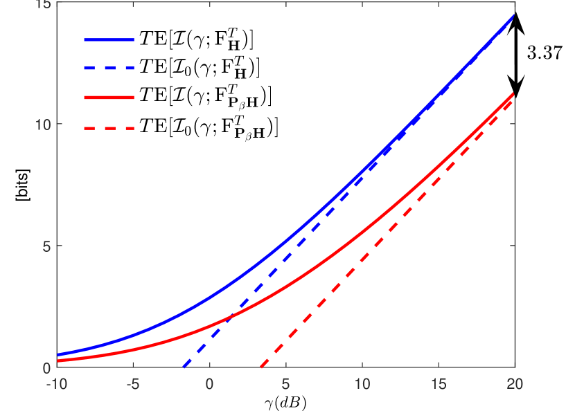
The normalized mutual information in (10
ℐ ( γ ; F 𝑯 T ) ℐ 𝛾 superscript subscript F 𝑯 𝑇
\displaystyle\mathcal{I}(\gamma;{\rm F}_{{\mathchoice{\mbox{\boldmath$\displaystyle H$}}{\mbox{\boldmath$\textstyle H$}}{\mbox{\boldmath$\scriptstyle H$}}{\mbox{\boldmath$\scriptscriptstyle H$}}}}^{T}) = α 𝑯 T ∫ log 2 ( γ x ) d F ~ 𝑯 T ( x ) ⏟ ℐ 0 ( γ ; F 𝑯 T ) absent subscript ⏟ superscript subscript 𝛼 𝑯 𝑇 subscript 2 𝛾 𝑥 differential-d subscript superscript ~ F 𝑇 𝑯 𝑥 subscript ℐ 0 𝛾 superscript subscript F 𝑯 𝑇
\displaystyle=\underbrace{\alpha_{\mathchoice{\mbox{\boldmath$\displaystyle H$}}{\mbox{\boldmath$\textstyle H$}}{\mbox{\boldmath$\scriptstyle H$}}{\mbox{\boldmath$\scriptscriptstyle H$}}}^{T}\int\log_{2}(\gamma x)\;{\rm d}{\tilde{\rm F}}^{T}_{{\mathchoice{\mbox{\boldmath$\displaystyle H$}}{\mbox{\boldmath$\textstyle H$}}{\mbox{\boldmath$\scriptstyle H$}}{\mbox{\boldmath$\scriptscriptstyle H$}}}}(x)}_{\mathcal{I}_{0}(\gamma;{\rm F}_{{\mathchoice{\mbox{\boldmath$\displaystyle H$}}{\mbox{\boldmath$\textstyle H$}}{\mbox{\boldmath$\scriptstyle H$}}{\mbox{\boldmath$\scriptscriptstyle H$}}}}^{T})}
+ α 𝑯 T ∫ log 2 ( 1 + 1 x γ ) d F ~ 𝑯 T ( x ) ⏟ Δ ℐ ( γ ; F 𝑯 T ) . subscript ⏟ superscript subscript 𝛼 𝑯 𝑇 subscript 2 1 1 𝑥 𝛾 differential-d subscript superscript ~ F 𝑇 𝑯 𝑥 Δ ℐ 𝛾 subscript superscript F 𝑇 𝑯
\displaystyle\quad+\underbrace{\alpha_{{\mathchoice{\mbox{\boldmath$\displaystyle H$}}{\mbox{\boldmath$\textstyle H$}}{\mbox{\boldmath$\scriptstyle H$}}{\mbox{\boldmath$\scriptscriptstyle H$}}}}^{T}\int\log_{2}\left(1+\frac{1}{x\gamma}\right)\;{\rm d}{\tilde{\rm F}}^{T}_{{\mathchoice{\mbox{\boldmath$\displaystyle H$}}{\mbox{\boldmath$\textstyle H$}}{\mbox{\boldmath$\scriptstyle H$}}{\mbox{\boldmath$\scriptscriptstyle H$}}}}(x)}_{\Delta\mathcal{I}(\gamma;{\rm F}^{T}_{{\mathchoice{\mbox{\boldmath$\displaystyle H$}}{\mbox{\boldmath$\textstyle H$}}{\mbox{\boldmath$\scriptstyle H$}}{\mbox{\boldmath$\scriptscriptstyle H$}}}})}. (19)
We refer to the first term ℐ 0 ( γ ; F 𝑯 T ) subscript ℐ 0 𝛾 subscript superscript F 𝑇 𝑯
\mathcal{I}_{0}(\gamma;{\rm F}^{T}_{{\mathchoice{\mbox{\boldmath$\displaystyle H$}}{\mbox{\boldmath$\textstyle H$}}{\mbox{\boldmath$\scriptstyle H$}}{\mbox{\boldmath$\scriptscriptstyle H$}}}}) multiplexing rate per transmit antenna. The factor α 𝑯 T superscript subscript 𝛼 𝑯 𝑇 \alpha_{\mathchoice{\mbox{\boldmath$\displaystyle H$}}{\mbox{\boldmath$\textstyle H$}}{\mbox{\boldmath$\scriptstyle H$}}{\mbox{\boldmath$\scriptscriptstyle H$}}}^{T} Δ ℐ ( γ ; F 𝑯 T ) Δ ℐ 𝛾 subscript superscript F 𝑇 𝑯
\Delta\mathcal{I}(\gamma;{\rm F}^{T}_{{\mathchoice{\mbox{\boldmath$\displaystyle H$}}{\mbox{\boldmath$\textstyle H$}}{\mbox{\boldmath$\scriptstyle H$}}{\mbox{\boldmath$\scriptscriptstyle H$}}}}) 19
lim γ → ∞ Δ ℐ ( γ ; F 𝑯 T ) = 0 . subscript → 𝛾 Δ ℐ 𝛾 subscript superscript F 𝑇 𝑯
0 \displaystyle\lim_{\gamma\to\infty}\Delta\mathcal{I}(\gamma;{\rm F}^{T}_{{\mathchoice{\mbox{\boldmath$\displaystyle H$}}{\mbox{\boldmath$\textstyle H$}}{\mbox{\boldmath$\scriptstyle H$}}{\mbox{\boldmath$\scriptscriptstyle H$}}}})=0. (20)
If 𝑯 † 𝑯 superscript 𝑯 † 𝑯 {\mathchoice{\mbox{\boldmath$\displaystyle H$}}{\mbox{\boldmath$\textstyle H$}}{\mbox{\boldmath$\scriptstyle H$}}{\mbox{\boldmath$\scriptscriptstyle H$}}}^{\dagger}{\mathchoice{\mbox{\boldmath$\displaystyle H$}}{\mbox{\boldmath$\textstyle H$}}{\mbox{\boldmath$\scriptstyle H$}}{\mbox{\boldmath$\scriptscriptstyle H$}}}
ℐ 0 ( γ ; F 𝑯 T ) subscript ℐ 0 𝛾 subscript superscript F 𝑇 𝑯
\displaystyle\mathcal{I}_{0}(\gamma;{\rm F}^{T}_{{\mathchoice{\mbox{\boldmath$\displaystyle H$}}{\mbox{\boldmath$\textstyle H$}}{\mbox{\boldmath$\scriptstyle H$}}{\mbox{\boldmath$\scriptscriptstyle H$}}}}) = 1 T log 2 det ( γ 𝑯 † 𝑯 ) absent 1 𝑇 subscript 2 𝛾 superscript 𝑯 † 𝑯 \displaystyle=\frac{1}{T}\log_{2}\det\left(\gamma{\mathchoice{\mbox{\boldmath$\displaystyle H$}}{\mbox{\boldmath$\textstyle H$}}{\mbox{\boldmath$\scriptstyle H$}}{\mbox{\boldmath$\scriptscriptstyle H$}}}^{\dagger}{\mathchoice{\mbox{\boldmath$\displaystyle H$}}{\mbox{\boldmath$\textstyle H$}}{\mbox{\boldmath$\scriptstyle H$}}{\mbox{\boldmath$\scriptscriptstyle H$}}}\right) (21)
Δ ℐ ( γ ; F 𝑯 T ) Δ ℐ 𝛾 subscript superscript F 𝑇 𝑯
\displaystyle\Delta\mathcal{I}(\gamma;{\rm F}^{T}_{{\mathchoice{\mbox{\boldmath$\displaystyle H$}}{\mbox{\boldmath$\textstyle H$}}{\mbox{\boldmath$\scriptstyle H$}}{\mbox{\boldmath$\scriptscriptstyle H$}}}}) = 1 T log 2 det ( 𝐈 + ( γ 𝑯 † 𝑯 ) − 𝟏 ) absent 1 𝑇 subscript 2 𝐈 superscript 𝛾 superscript 𝑯 † 𝑯 1 \displaystyle=\frac{1}{T}\log_{2}\det\left(\bf I+{(\gamma{\mathchoice{\mbox{\boldmath$\displaystyle H$}}{\mbox{\boldmath$\textstyle H$}}{\mbox{\boldmath$\scriptstyle H$}}{\mbox{\boldmath$\scriptscriptstyle H$}}}^{\dagger}{\mathchoice{\mbox{\boldmath$\displaystyle H$}}{\mbox{\boldmath$\textstyle H$}}{\mbox{\boldmath$\scriptstyle H$}}{\mbox{\boldmath$\scriptscriptstyle H$}}})^{-1}}\right) (22)
with 𝐈 𝐈 \bf I
The affine approximation of the ergodic mutual information at high SNR introduced in [1 ] , see also [5 , Eq. (9)] for a compact formulation of it, coincides with the ergodic formulation of our definition of the multiplexing rate.
We next uncover a fundamental link between the mutual information and the multiplexing rate. This result makes use of the minimum-mean-square-error (MMSE) achieved by the optimal receiver for (8
η 𝑯 T ( γ ) ≜ ∫ dF 𝑯 T ( x ) 1 + γ x . ≜ superscript subscript 𝜂 𝑯 𝑇 𝛾 subscript superscript dF 𝑇 𝑯 𝑥 1 𝛾 𝑥 \eta_{{\mathchoice{\mbox{\boldmath$\displaystyle H$}}{\mbox{\boldmath$\textstyle H$}}{\mbox{\boldmath$\scriptstyle H$}}{\mbox{\boldmath$\scriptscriptstyle H$}}}}^{T}(\gamma)\triangleq\int\frac{{\rm dF}^{T}_{{\mathchoice{\mbox{\boldmath$\displaystyle H$}}{\mbox{\boldmath$\textstyle H$}}{\mbox{\boldmath$\scriptstyle H$}}{\mbox{\boldmath$\scriptscriptstyle H$}}}}(x)}{1+\gamma x}. (23)
Clearly, η 𝑯 T ( γ ) superscript subscript 𝜂 𝑯 𝑇 𝛾 \eta_{{\mathchoice{\mbox{\boldmath$\displaystyle H$}}{\mbox{\boldmath$\textstyle H$}}{\mbox{\boldmath$\scriptstyle H$}}{\mbox{\boldmath$\scriptscriptstyle H$}}}}^{T}(\gamma) γ 𝛾 \gamma ( 1 − α 𝑯 T , 1 ) 1 superscript subscript 𝛼 𝑯 𝑇 1 (1-\alpha_{{\mathchoice{\mbox{\boldmath$\displaystyle H$}}{\mbox{\boldmath$\textstyle H$}}{\mbox{\boldmath$\scriptstyle H$}}{\mbox{\boldmath$\scriptscriptstyle H$}}}}^{T},1) [9 ] .
Theorem 1
Define
f 𝑯 ( x ) ≜ H ( x ) − ∫ 0 x log 2 S 𝑯 T ( − z ) d z , 0 ≤ x ≤ α 𝑯 T . formulae-sequence ≜ subscript 𝑓 𝑯 𝑥 𝐻 𝑥 superscript subscript 0 𝑥 subscript 2 subscript superscript S 𝑇 𝑯 𝑧 differential-d 𝑧 0 𝑥 superscript subscript 𝛼 𝑯 𝑇 f_{{\mathchoice{\mbox{\boldmath$\displaystyle H$}}{\mbox{\boldmath$\textstyle H$}}{\mbox{\boldmath$\scriptstyle H$}}{\mbox{\boldmath$\scriptscriptstyle H$}}}}(x)\triangleq H(x)-\int_{0}^{x}\log_{2}{\rm S}^{T}_{{\mathchoice{\mbox{\boldmath$\displaystyle H$}}{\mbox{\boldmath$\textstyle H$}}{\mbox{\boldmath$\scriptstyle H$}}{\mbox{\boldmath$\scriptscriptstyle H$}}}}(-z)\;{\rm d}z,\quad 0\leq x\leq\alpha_{{\mathchoice{\mbox{\boldmath$\displaystyle H$}}{\mbox{\boldmath$\textstyle H$}}{\mbox{\boldmath$\scriptstyle H$}}{\mbox{\boldmath$\scriptscriptstyle H$}}}}^{T}. (24)
Then, we have
ℐ ( γ ; F 𝑯 T ) ℐ 𝛾 subscript superscript F 𝑇 𝑯
\displaystyle\mathcal{I}(\gamma;{\rm F}^{T}_{{\mathchoice{\mbox{\boldmath$\displaystyle H$}}{\mbox{\boldmath$\textstyle H$}}{\mbox{\boldmath$\scriptstyle H$}}{\mbox{\boldmath$\scriptscriptstyle H$}}}}) = f 𝑯 ( 1 − η 𝑯 T ) + ( 1 − η 𝑯 T ) log 2 γ absent subscript 𝑓 𝑯 1 subscript superscript 𝜂 𝑇 𝑯 1 superscript subscript 𝜂 𝑯 𝑇 subscript 2 𝛾 \displaystyle=f_{{\mathchoice{\mbox{\boldmath$\displaystyle H$}}{\mbox{\boldmath$\textstyle H$}}{\mbox{\boldmath$\scriptstyle H$}}{\mbox{\boldmath$\scriptscriptstyle H$}}}}(1-\eta^{T}_{{\mathchoice{\mbox{\boldmath$\displaystyle H$}}{\mbox{\boldmath$\textstyle H$}}{\mbox{\boldmath$\scriptstyle H$}}{\mbox{\boldmath$\scriptscriptstyle H$}}}})+(1-\eta_{{\mathchoice{\mbox{\boldmath$\displaystyle H$}}{\mbox{\boldmath$\textstyle H$}}{\mbox{\boldmath$\scriptstyle H$}}{\mbox{\boldmath$\scriptscriptstyle H$}}}}^{T})\log_{2}\gamma (25)
ℐ 0 ( γ ; F 𝑯 T ) subscript ℐ 0 𝛾 subscript superscript F 𝑇 𝑯
\displaystyle\mathcal{I}_{0}(\gamma;{\rm F}^{T}_{{\mathchoice{\mbox{\boldmath$\displaystyle H$}}{\mbox{\boldmath$\textstyle H$}}{\mbox{\boldmath$\scriptstyle H$}}{\mbox{\boldmath$\scriptscriptstyle H$}}}}) = f 𝑯 ( α 𝑯 T ) + α 𝑯 T log 2 γ . absent subscript 𝑓 𝑯 subscript superscript 𝛼 𝑇 𝑯 superscript subscript 𝛼 𝑯 𝑇 subscript 2 𝛾 \displaystyle=f_{{\mathchoice{\mbox{\boldmath$\displaystyle H$}}{\mbox{\boldmath$\textstyle H$}}{\mbox{\boldmath$\scriptstyle H$}}{\mbox{\boldmath$\scriptscriptstyle H$}}}}(\alpha^{T}_{{\mathchoice{\mbox{\boldmath$\displaystyle H$}}{\mbox{\boldmath$\textstyle H$}}{\mbox{\boldmath$\scriptstyle H$}}{\mbox{\boldmath$\scriptscriptstyle H$}}}})+\alpha_{{\mathchoice{\mbox{\boldmath$\displaystyle H$}}{\mbox{\boldmath$\textstyle H$}}{\mbox{\boldmath$\scriptstyle H$}}{\mbox{\boldmath$\scriptscriptstyle H$}}}}^{T}\log_{2}\gamma. (26)
For short we write η 𝐇 T superscript subscript 𝜂 𝐇 𝑇 \eta_{{\mathchoice{\mbox{\boldmath$\displaystyle H$}}{\mbox{\boldmath$\textstyle H$}}{\mbox{\boldmath$\scriptstyle H$}}{\mbox{\boldmath$\scriptscriptstyle H$}}}}^{T} η 𝐇 T ( γ ) superscript subscript 𝜂 𝐇 𝑇 𝛾 \eta_{{\mathchoice{\mbox{\boldmath$\displaystyle H$}}{\mbox{\boldmath$\textstyle H$}}{\mbox{\boldmath$\scriptstyle H$}}{\mbox{\boldmath$\scriptscriptstyle H$}}}}^{T}(\gamma) 25
Note that by definition the function f 𝑯 ( x ) subscript 𝑓 𝑯 𝑥 f_{{\mathchoice{\mbox{\boldmath$\displaystyle H$}}{\mbox{\boldmath$\textstyle H$}}{\mbox{\boldmath$\scriptstyle H$}}{\mbox{\boldmath$\scriptscriptstyle H$}}}}(x) 24 α 𝑯 T superscript subscript 𝛼 𝑯 𝑇 \alpha_{{\mathchoice{\mbox{\boldmath$\displaystyle H$}}{\mbox{\boldmath$\textstyle H$}}{\mbox{\boldmath$\scriptstyle H$}}{\mbox{\boldmath$\scriptscriptstyle H$}}}}^{T} S 𝑯 T ( z ) superscript subscript S 𝑯 𝑇 𝑧 {\rm S}_{{\mathchoice{\mbox{\boldmath$\displaystyle H$}}{\mbox{\boldmath$\textstyle H$}}{\mbox{\boldmath$\scriptstyle H$}}{\mbox{\boldmath$\scriptscriptstyle H$}}}}^{{T}}(z) 1 η 𝑯 T superscript subscript 𝜂 𝑯 𝑇 \eta_{{\mathchoice{\mbox{\boldmath$\displaystyle H$}}{\mbox{\boldmath$\textstyle H$}}{\mbox{\boldmath$\scriptstyle H$}}{\mbox{\boldmath$\scriptscriptstyle H$}}}}^{T} η 𝑯 T superscript subscript 𝜂 𝑯 𝑇 \eta_{{\mathchoice{\mbox{\boldmath$\displaystyle H$}}{\mbox{\boldmath$\textstyle H$}}{\mbox{\boldmath$\scriptstyle H$}}{\mbox{\boldmath$\scriptscriptstyle H$}}}}^{T} 1 − α 𝑯 T 1 superscript subscript 𝛼 𝑯 𝑇 1-\alpha_{{\mathchoice{\mbox{\boldmath$\displaystyle H$}}{\mbox{\boldmath$\textstyle H$}}{\mbox{\boldmath$\scriptstyle H$}}{\mbox{\boldmath$\scriptscriptstyle H$}}}}^{T} 1 2 α 𝑯 T superscript subscript 𝛼 𝑯 𝑇 \alpha_{{\mathchoice{\mbox{\boldmath$\displaystyle H$}}{\mbox{\boldmath$\textstyle H$}}{\mbox{\boldmath$\scriptstyle H$}}{\mbox{\boldmath$\scriptscriptstyle H$}}}}^{T} α 𝑯 T superscript subscript 𝛼 𝑯 𝑇 \alpha_{{\mathchoice{\mbox{\boldmath$\displaystyle H$}}{\mbox{\boldmath$\textstyle H$}}{\mbox{\boldmath$\scriptstyle H$}}{\mbox{\boldmath$\scriptscriptstyle H$}}}}^{T} 1 − η 𝑯 T 1 superscript subscript 𝜂 𝑯 𝑇 1-\eta_{{\mathchoice{\mbox{\boldmath$\displaystyle H$}}{\mbox{\boldmath$\textstyle H$}}{\mbox{\boldmath$\scriptstyle H$}}{\mbox{\boldmath$\scriptscriptstyle H$}}}}^{T} f 𝑯 subscript 𝑓 𝑯 f_{\mathchoice{\mbox{\boldmath$\displaystyle H$}}{\mbox{\boldmath$\textstyle H$}}{\mbox{\boldmath$\scriptstyle H$}}{\mbox{\boldmath$\scriptscriptstyle H$}}} α 𝑯 T superscript subscript 𝛼 𝑯 𝑇 \alpha_{{\mathchoice{\mbox{\boldmath$\displaystyle H$}}{\mbox{\boldmath$\textstyle H$}}{\mbox{\boldmath$\scriptstyle H$}}{\mbox{\boldmath$\scriptscriptstyle H$}}}}^{T} 1 − η 𝑯 T 1 superscript subscript 𝜂 𝑯 𝑇 1-\eta_{{\mathchoice{\mbox{\boldmath$\displaystyle H$}}{\mbox{\boldmath$\textstyle H$}}{\mbox{\boldmath$\scriptstyle H$}}{\mbox{\boldmath$\scriptscriptstyle H$}}}}^{T}
If any probability distribution function with support in [ 0 , ∞ ) 0 [0,\infty) F F \rm F F 𝑯 T superscript subscript F 𝑯 𝑇 {\rm F}_{{\mathchoice{\mbox{\boldmath$\displaystyle H$}}{\mbox{\boldmath$\textstyle H$}}{\mbox{\boldmath$\scriptstyle H$}}{\mbox{\boldmath$\scriptscriptstyle H$}}}}^{T} 19 25 26 ℐ ( γ ; F ) ℐ 𝛾 F
\mathcal{I}(\gamma;{\rm F}) log ( x ) 𝑥 \log(x) F ~ ~ F {\rm\tilde{F}} ℐ ( γ ; F ) ℐ 𝛾 F
\mathcal{I}(\gamma;{\rm F}) Δ ℐ ( γ ; F ) Δ ℐ 𝛾 F
\Delta\mathcal{I}(\gamma;{\rm F}) 171 173 F 𝑯 subscript F 𝑯 {\rm F}_{{\mathchoice{\mbox{\boldmath$\displaystyle H$}}{\mbox{\boldmath$\textstyle H$}}{\mbox{\boldmath$\scriptstyle H$}}{\mbox{\boldmath$\scriptscriptstyle H$}}}} F 𝑯 T subscript superscript F 𝑇 𝑯 {\rm F}^{T}_{{\mathchoice{\mbox{\boldmath$\displaystyle H$}}{\mbox{\boldmath$\textstyle H$}}{\mbox{\boldmath$\scriptstyle H$}}{\mbox{\boldmath$\scriptscriptstyle H$}}}} ℐ ( γ ; F 𝑯 ) ℐ 𝛾 subscript F 𝑯
\mathcal{I}(\gamma;{\rm F}_{{\mathchoice{\mbox{\boldmath$\displaystyle H$}}{\mbox{\boldmath$\textstyle H$}}{\mbox{\boldmath$\scriptstyle H$}}{\mbox{\boldmath$\scriptscriptstyle H$}}}}) ℐ 0 ( γ ; F 𝑯 ) subscript ℐ 0 𝛾 subscript F 𝑯
\mathcal{I}_{0}(\gamma;{\rm F}_{{\mathchoice{\mbox{\boldmath$\displaystyle H$}}{\mbox{\boldmath$\textstyle H$}}{\mbox{\boldmath$\scriptstyle H$}}{\mbox{\boldmath$\scriptscriptstyle H$}}}}) ℐ ( γ ; F 𝑯 T ) ℐ 𝛾 subscript superscript F 𝑇 𝑯
\mathcal{I}(\gamma;{\rm F}^{T}_{{\mathchoice{\mbox{\boldmath$\displaystyle H$}}{\mbox{\boldmath$\textstyle H$}}{\mbox{\boldmath$\scriptstyle H$}}{\mbox{\boldmath$\scriptscriptstyle H$}}}}) ℐ 0 ( γ ; F 𝑯 T ) subscript ℐ 0 𝛾 subscript superscript F 𝑇 𝑯
\mathcal{I}_{0}(\gamma;{\rm F}^{T}_{{\mathchoice{\mbox{\boldmath$\displaystyle H$}}{\mbox{\boldmath$\textstyle H$}}{\mbox{\boldmath$\scriptstyle H$}}{\mbox{\boldmath$\scriptscriptstyle H$}}}}) ℐ ( γ ; F 𝑯 ) ℐ 𝛾 subscript F 𝑯
\mathcal{I}(\gamma;{\rm F}_{{\mathchoice{\mbox{\boldmath$\displaystyle H$}}{\mbox{\boldmath$\textstyle H$}}{\mbox{\boldmath$\scriptstyle H$}}{\mbox{\boldmath$\scriptscriptstyle H$}}}}) ℐ 0 ( γ ; F 𝑯 ) subscript ℐ 0 𝛾 subscript F 𝑯
\mathcal{I}_{0}(\gamma;{\rm F}_{{\mathchoice{\mbox{\boldmath$\displaystyle H$}}{\mbox{\boldmath$\textstyle H$}}{\mbox{\boldmath$\scriptstyle H$}}{\mbox{\boldmath$\scriptscriptstyle H$}}}})
It is well-known that the S-transform of the LED of the product of asymptotically free matrices is the product of the respective S-transforms of the LEDs of these matrices. Therefore, for MIMO channel matrices that involve a compound structure, Theorem 1 analytically calculate the large-system limits of the mutual information and multiplexing rate in terms of the large-system limits of the MMSE and the multiplexing gain . We next address two relevant random matrix ensembles that share this structure.
Example 1
We consider the concatenation of vector-valued fading channels described in [13 ] . Specifically, we assume that the channel matrix 𝐇 𝐇 \textstyle H
𝑯 = 𝑿 N 𝑿 N − 1 ⋯ 𝑿 2 𝑿 1 𝑯 subscript 𝑿 𝑁 subscript 𝑿 𝑁 1 ⋯ subscript 𝑿 2 subscript 𝑿 1 {\mathchoice{\mbox{\boldmath$\displaystyle{\mathchoice{\mbox{\boldmath$\displaystyle H$}}{\mbox{\boldmath$\textstyle H$}}{\mbox{\boldmath$\scriptstyle H$}}{\mbox{\boldmath$\scriptscriptstyle H$}}}$}}{\mbox{\boldmath$\textstyle{\mathchoice{\mbox{\boldmath$\displaystyle H$}}{\mbox{\boldmath$\textstyle H$}}{\mbox{\boldmath$\scriptstyle H$}}{\mbox{\boldmath$\scriptscriptstyle H$}}}$}}{\mbox{\boldmath$\scriptstyle{\mathchoice{\mbox{\boldmath$\displaystyle H$}}{\mbox{\boldmath$\textstyle H$}}{\mbox{\boldmath$\scriptstyle H$}}{\mbox{\boldmath$\scriptscriptstyle H$}}}$}}{\mbox{\boldmath$\scriptscriptstyle{\mathchoice{\mbox{\boldmath$\displaystyle H$}}{\mbox{\boldmath$\textstyle H$}}{\mbox{\boldmath$\scriptstyle H$}}{\mbox{\boldmath$\scriptscriptstyle H$}}}$}}}={\mathchoice{\mbox{\boldmath$\displaystyle X$}}{\mbox{\boldmath$\textstyle X$}}{\mbox{\boldmath$\scriptstyle X$}}{\mbox{\boldmath$\scriptscriptstyle X$}}}_{N}{\mathchoice{\mbox{\boldmath$\displaystyle X$}}{\mbox{\boldmath$\textstyle X$}}{\mbox{\boldmath$\scriptstyle X$}}{\mbox{\boldmath$\scriptscriptstyle X$}}}_{N-1}\cdots{\mathchoice{\mbox{\boldmath$\displaystyle X$}}{\mbox{\boldmath$\textstyle X$}}{\mbox{\boldmath$\scriptstyle X$}}{\mbox{\boldmath$\scriptscriptstyle X$}}}_{2}{\mathchoice{\mbox{\boldmath$\displaystyle X$}}{\mbox{\boldmath$\textstyle X$}}{\mbox{\boldmath$\scriptstyle X$}}{\mbox{\boldmath$\scriptscriptstyle X$}}}_{1} (27)
where the entries of the K n × K n − 1 subscript 𝐾 𝑛 subscript 𝐾 𝑛 1 K_{n}\times K_{n-1} 𝐗 n subscript 𝐗 𝑛 {\mathchoice{\mbox{\boldmath$\displaystyle X$}}{\mbox{\boldmath$\textstyle X$}}{\mbox{\boldmath$\scriptstyle X$}}{\mbox{\boldmath$\scriptscriptstyle X$}}}_{n} 1 / K n 1 subscript 𝐾 𝑛 1/K_{n} n ∈ [ 1 , N ] 𝑛 1 𝑁 n\in[1,N] ρ n ≜ K n / K 0 ≜ subscript 𝜌 𝑛 subscript 𝐾 𝑛 subscript 𝐾 0 \rho_{n}\triangleq K_{n}/K_{0} n ∈ [ 1 , N ] 𝑛 1 𝑁 n\in[1,N] K n → ∞ → subscript 𝐾 𝑛 K_{n}\to\infty η 𝐇 subscript 𝜂 𝐇 \eta_{\mathchoice{\mbox{\boldmath$\displaystyle H$}}{\mbox{\boldmath$\textstyle H$}}{\mbox{\boldmath$\scriptstyle H$}}{\mbox{\boldmath$\scriptscriptstyle H$}}} η 𝐇 T superscript subscript 𝜂 𝐇 𝑇 \eta_{\mathchoice{\mbox{\boldmath$\displaystyle H$}}{\mbox{\boldmath$\textstyle H$}}{\mbox{\boldmath$\scriptstyle H$}}{\mbox{\boldmath$\scriptscriptstyle H$}}}^{T} 1
ℐ ( γ ; F 𝑯 ) = H ( η 𝑯 ) + ( 1 − η 𝑯 ) ( log 2 γ − N log 2 e ) ℐ 𝛾 subscript F 𝑯
𝐻 subscript 𝜂 𝑯 1 subscript 𝜂 𝑯 subscript 2 𝛾 𝑁 subscript 2 𝑒 \displaystyle\mathcal{I}(\gamma;{\rm F}_{{\mathchoice{\mbox{\boldmath$\displaystyle H$}}{\mbox{\boldmath$\textstyle H$}}{\mbox{\boldmath$\scriptstyle H$}}{\mbox{\boldmath$\scriptscriptstyle H$}}}})=H(\eta_{\mathchoice{\mbox{\boldmath$\displaystyle H$}}{\mbox{\boldmath$\textstyle H$}}{\mbox{\boldmath$\scriptstyle H$}}{\mbox{\boldmath$\scriptscriptstyle H$}}})+(1-\eta_{{\mathchoice{\mbox{\boldmath$\displaystyle H$}}{\mbox{\boldmath$\textstyle H$}}{\mbox{\boldmath$\scriptstyle H$}}{\mbox{\boldmath$\scriptscriptstyle H$}}}})(\log_{2}\gamma-N\log_{2}e)
+ ( 1 − η 𝑯 ) [ ∑ n = 1 N ρ n 1 − η 𝑯 H ( 1 − η 𝑯 ρ n ) + log 2 1 − η 𝑯 ρ n ] . 1 subscript 𝜂 𝑯 delimited-[] superscript subscript 𝑛 1 𝑁 subscript 𝜌 𝑛 1 subscript 𝜂 𝑯 𝐻 1 subscript 𝜂 𝑯 subscript 𝜌 𝑛 subscript 2 1 subscript 𝜂 𝑯 subscript 𝜌 𝑛 \displaystyle+(1-\eta_{{\mathchoice{\mbox{\boldmath$\displaystyle H$}}{\mbox{\boldmath$\textstyle H$}}{\mbox{\boldmath$\scriptstyle H$}}{\mbox{\boldmath$\scriptscriptstyle H$}}}})\left[\sum_{n=1}^{N}\frac{\rho_{n}}{1-\eta_{\mathchoice{\mbox{\boldmath$\displaystyle H$}}{\mbox{\boldmath$\textstyle H$}}{\mbox{\boldmath$\scriptstyle H$}}{\mbox{\boldmath$\scriptscriptstyle H$}}}}H\left(\frac{1-\eta_{\mathchoice{\mbox{\boldmath$\displaystyle H$}}{\mbox{\boldmath$\textstyle H$}}{\mbox{\boldmath$\scriptstyle H$}}{\mbox{\boldmath$\scriptscriptstyle H$}}}}{\rho_{n}}\right)+\log_{2}\frac{1-\eta_{\mathchoice{\mbox{\boldmath$\displaystyle H$}}{\mbox{\boldmath$\textstyle H$}}{\mbox{\boldmath$\scriptstyle H$}}{\mbox{\boldmath$\scriptscriptstyle H$}}}}{\rho_{n}}\right]. (28)
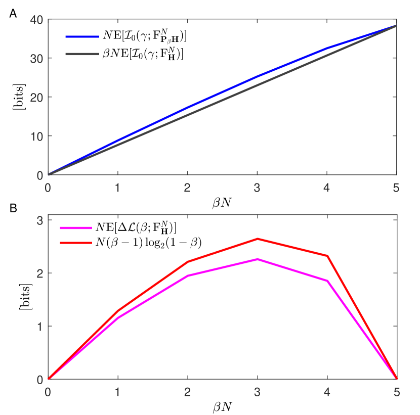
Furthermore, as regards the multiplexing rate, we have
ℐ 0 ( γ ; F 𝑯 ) = subscript ℐ 0 𝛾 subscript F 𝑯
absent \displaystyle\mathcal{I}_{0}(\gamma;{\rm F}_{{\mathchoice{\mbox{\boldmath$\displaystyle H$}}{\mbox{\boldmath$\textstyle H$}}{\mbox{\boldmath$\scriptstyle H$}}{\mbox{\boldmath$\scriptscriptstyle H$}}}})= H ( α 𝑯 ) + α 𝑯 ( log 2 γ − N log 2 e ) 𝐻 subscript 𝛼 𝑯 subscript 𝛼 𝑯 subscript 2 𝛾 𝑁 subscript 2 𝑒 \displaystyle H(\alpha_{\mathchoice{\mbox{\boldmath$\displaystyle H$}}{\mbox{\boldmath$\textstyle H$}}{\mbox{\boldmath$\scriptstyle H$}}{\mbox{\boldmath$\scriptscriptstyle H$}}})+\alpha_{{\mathchoice{\mbox{\boldmath$\displaystyle H$}}{\mbox{\boldmath$\textstyle H$}}{\mbox{\boldmath$\scriptstyle H$}}{\mbox{\boldmath$\scriptscriptstyle H$}}}}(\log_{2}\gamma-N\log_{2}e)
+ α 𝑯 [ ∑ n = 1 N ρ n α 𝑯 H ( α 𝑯 ρ n ) + log 2 α 𝑯 ρ n ] subscript 𝛼 𝑯 delimited-[] superscript subscript 𝑛 1 𝑁 subscript 𝜌 𝑛 subscript 𝛼 𝑯 𝐻 subscript 𝛼 𝑯 subscript 𝜌 𝑛 subscript 2 subscript 𝛼 𝑯 subscript 𝜌 𝑛 \displaystyle+\alpha_{{\mathchoice{\mbox{\boldmath$\displaystyle H$}}{\mbox{\boldmath$\textstyle H$}}{\mbox{\boldmath$\scriptstyle H$}}{\mbox{\boldmath$\scriptscriptstyle H$}}}}\left[\sum_{n=1}^{N}\frac{\rho_{n}}{\alpha_{\mathchoice{\mbox{\boldmath$\displaystyle H$}}{\mbox{\boldmath$\textstyle H$}}{\mbox{\boldmath$\scriptstyle H$}}{\mbox{\boldmath$\scriptscriptstyle H$}}}}H\left(\frac{\alpha_{\mathchoice{\mbox{\boldmath$\displaystyle H$}}{\mbox{\boldmath$\textstyle H$}}{\mbox{\boldmath$\scriptstyle H$}}{\mbox{\boldmath$\scriptscriptstyle H$}}}}{\rho_{n}}\right)+\log_{2}\frac{\alpha_{\mathchoice{\mbox{\boldmath$\displaystyle H$}}{\mbox{\boldmath$\textstyle H$}}{\mbox{\boldmath$\scriptstyle H$}}{\mbox{\boldmath$\scriptscriptstyle H$}}}}{\rho_{n}}\right] (29)
with α 𝐇 = min ( 1 , ρ 1 , ⋯ , ρ N ) subscript 𝛼 𝐇 1 subscript 𝜌 1 ⋯ subscript 𝜌 𝑁 \alpha_{{\mathchoice{\mbox{\boldmath$\displaystyle H$}}{\mbox{\boldmath$\textstyle H$}}{\mbox{\boldmath$\scriptstyle H$}}{\mbox{\boldmath$\scriptscriptstyle H$}}}}=\min(1,\rho_{1},\cdots,\rho_{N})
Example 2
We consider a Jacobi matrix ensemble, see e.g. [14 ] , [15 ] , which find application in the context of optical MIMO communications [16 ] ,[17 ] . Accordingly, the channel matrix factorizes as
𝑯 = 𝑷 β 2 𝐔 𝐏 β 1 † 𝑯 subscript 𝑷 subscript 𝛽 2 superscript subscript 𝐔 𝐏 subscript 𝛽 1 † {\mathchoice{\mbox{\boldmath$\displaystyle H$}}{\mbox{\boldmath$\textstyle H$}}{\mbox{\boldmath$\scriptstyle H$}}{\mbox{\boldmath$\scriptscriptstyle H$}}}={\mathchoice{\mbox{\boldmath$\displaystyle P$}}{\mbox{\boldmath$\textstyle P$}}{\mbox{\boldmath$\scriptstyle P$}}{\mbox{\boldmath$\scriptscriptstyle P$}}}_{\beta_{2}}{\mathchoice{\mbox{\boldmath$\displaystyle U$}}{\mbox{\boldmath$\textstyle U$}}{\mbox{\boldmath$\scriptstyle U$}}{\mbox{\boldmath$\scriptscriptstyle U$}}}{\mathchoice{\mbox{\boldmath$\displaystyle P$}}{\mbox{\boldmath$\textstyle P$}}{\mbox{\boldmath$\scriptstyle P$}}{\mbox{\boldmath$\scriptscriptstyle P$}}}_{\beta_{1}}^{\dagger} (30)
where 𝐔 𝐔 \textstyle U N × N 𝑁 𝑁 N\times N 1
ℐ ( γ ; F 𝑯 ) = ℐ 𝛾 subscript F 𝑯
absent \displaystyle\mathcal{I}(\gamma;{\rm F}_{{\mathchoice{\mbox{\boldmath$\displaystyle H$}}{\mbox{\boldmath$\textstyle H$}}{\mbox{\boldmath$\scriptstyle H$}}{\mbox{\boldmath$\scriptscriptstyle H$}}}})= H ( η 𝑯 ) + ( 1 − η 𝑯 ) log 2 γ 𝐻 subscript 𝜂 𝑯 1 subscript 𝜂 𝑯 subscript 2 𝛾 \displaystyle H(\eta_{\mathchoice{\mbox{\boldmath$\displaystyle H$}}{\mbox{\boldmath$\textstyle H$}}{\mbox{\boldmath$\scriptstyle H$}}{\mbox{\boldmath$\scriptscriptstyle H$}}})+(1-\eta_{{\mathchoice{\mbox{\boldmath$\displaystyle H$}}{\mbox{\boldmath$\textstyle H$}}{\mbox{\boldmath$\scriptstyle H$}}{\mbox{\boldmath$\scriptscriptstyle H$}}}})\log_{2}\gamma
− H ( β 1 ( 1 − η 𝑯 ) ) β 1 + β 2 β 1 H ( β 1 β 2 ( 1 − η 𝑯 ) ) 𝐻 subscript 𝛽 1 1 subscript 𝜂 𝑯 subscript 𝛽 1 subscript 𝛽 2 subscript 𝛽 1 𝐻 subscript 𝛽 1 subscript 𝛽 2 1 subscript 𝜂 𝑯 \displaystyle-\frac{H(\beta_{1}(1-\eta_{{\mathchoice{\mbox{\boldmath$\displaystyle H$}}{\mbox{\boldmath$\textstyle H$}}{\mbox{\boldmath$\scriptstyle H$}}{\mbox{\boldmath$\scriptscriptstyle H$}}}}))}{\beta_{1}}+\frac{\beta_{2}}{\beta_{1}}H\left(\frac{\beta_{1}}{\beta_{2}}(1-\eta_{{\mathchoice{\mbox{\boldmath$\displaystyle H$}}{\mbox{\boldmath$\textstyle H$}}{\mbox{\boldmath$\scriptstyle H$}}{\mbox{\boldmath$\scriptscriptstyle H$}}}})\right) (31)
where η 𝐇 = η 𝐇 ( γ ) subscript 𝜂 𝐇 subscript 𝜂 𝐇 𝛾 \eta_{{\mathchoice{\mbox{\boldmath$\displaystyle H$}}{\mbox{\boldmath$\textstyle H$}}{\mbox{\boldmath$\scriptstyle H$}}{\mbox{\boldmath$\scriptscriptstyle H$}}}}=\eta_{{\mathchoice{\mbox{\boldmath$\displaystyle H$}}{\mbox{\boldmath$\textstyle H$}}{\mbox{\boldmath$\scriptstyle H$}}{\mbox{\boldmath$\scriptscriptstyle H$}}}}(\gamma)
η 𝑯 ( γ ) = 1 + − ( 1 + κ γ ) + ( 1 + κ γ ) 2 − 4 β 1 β 2 γ ( 1 + γ ) 2 β 1 ( 1 + γ ) subscript 𝜂 𝑯 𝛾 1 1 𝜅 𝛾 superscript 1 𝜅 𝛾 2 4 subscript 𝛽 1 subscript 𝛽 2 𝛾 1 𝛾 2 subscript 𝛽 1 1 𝛾 \eta_{\mathchoice{\mbox{\boldmath$\displaystyle H$}}{\mbox{\boldmath$\textstyle H$}}{\mbox{\boldmath$\scriptstyle H$}}{\mbox{\boldmath$\scriptscriptstyle H$}}}(\gamma)=1+\frac{-(1+\kappa\gamma)+\sqrt{(1+\kappa\gamma)^{2}-4\beta_{1}\beta_{2}\gamma(1+\gamma)}}{2\beta_{1}(1+\gamma)} (32)
with κ ≜ β 1 + β 2 ≜ 𝜅 subscript 𝛽 1 subscript 𝛽 2 \kappa\triangleq\beta_{1}+\beta_{2}
ℐ 0 ( γ ; F 𝑯 ) = subscript ℐ 0 𝛾 subscript F 𝑯
absent \displaystyle\mathcal{I}_{0}(\gamma;{\rm F}_{{\mathchoice{\mbox{\boldmath$\displaystyle H$}}{\mbox{\boldmath$\textstyle H$}}{\mbox{\boldmath$\scriptstyle H$}}{\mbox{\boldmath$\scriptscriptstyle H$}}}})= H ( α 𝑯 ) + α 𝑯 log 2 γ 𝐻 subscript 𝛼 𝑯 subscript 𝛼 𝑯 subscript 2 𝛾 \displaystyle H(\alpha_{{\mathchoice{\mbox{\boldmath$\displaystyle H$}}{\mbox{\boldmath$\textstyle H$}}{\mbox{\boldmath$\scriptstyle H$}}{\mbox{\boldmath$\scriptscriptstyle H$}}}})+\alpha_{{\mathchoice{\mbox{\boldmath$\displaystyle H$}}{\mbox{\boldmath$\textstyle H$}}{\mbox{\boldmath$\scriptstyle H$}}{\mbox{\boldmath$\scriptscriptstyle H$}}}}\log_{2}\gamma
− H ( β 1 α 𝑯 ) β 1 + β 2 β 1 H ( β 1 β 2 α 𝑯 ) 𝐻 subscript 𝛽 1 subscript 𝛼 𝑯 subscript 𝛽 1 subscript 𝛽 2 subscript 𝛽 1 𝐻 subscript 𝛽 1 subscript 𝛽 2 subscript 𝛼 𝑯 \displaystyle-\frac{H(\beta_{1}\alpha_{{\mathchoice{\mbox{\boldmath$\displaystyle H$}}{\mbox{\boldmath$\textstyle H$}}{\mbox{\boldmath$\scriptstyle H$}}{\mbox{\boldmath$\scriptscriptstyle H$}}}})}{\beta_{1}}+\frac{\beta_{2}}{\beta_{1}}H\left(\frac{\beta_{1}}{\beta_{2}}\alpha_{{\mathchoice{\mbox{\boldmath$\displaystyle H$}}{\mbox{\boldmath$\textstyle H$}}{\mbox{\boldmath$\scriptstyle H$}}{\mbox{\boldmath$\scriptscriptstyle H$}}}}\right) (33)
with α 𝐇 = min ( 1 , β 2 / β 1 ) subscript 𝛼 𝐇 1 subscript 𝛽 2 subscript 𝛽 1 \alpha_{{\mathchoice{\mbox{\boldmath$\displaystyle H$}}{\mbox{\boldmath$\textstyle H$}}{\mbox{\boldmath$\scriptstyle H$}}{\mbox{\boldmath$\scriptscriptstyle H$}}}}=\min(1,\beta_{2}/\beta_{1})
V The Universal Rate Loss
In Section 1 we underlined the following misinterpretation of mutual information: when the number of antennas (at either the transmit or receive side) varies, with the minimum of the system dimensions kept fixed, the mutual information does not vary at high SNR. It is the goal of this section to elucidate this misinterpretation. To do so we need to distinguish between two cases as to reference system (8 T ≤ R 𝑇 𝑅 T\leq R T ≥ R 𝑇 𝑅 T\geq R
V-A Case (i) – Removing receive antennas
We remove a fraction ( 1 − β ) 1 𝛽 (1-\beta) 8 12 β ≥ ϕ ≜ T / R 𝛽 italic-ϕ ≜ 𝑇 𝑅 \beta\geq\phi\triangleq T/R min ( T , β R ) = T 𝑇 𝛽 𝑅 𝑇 \min(T,\beta R)=T T ℐ ( γ ; F 𝑯 T ) − T ℐ ( γ ; F 𝑷 β 𝑯 T ) 𝑇 ℐ 𝛾 subscript superscript F 𝑇 𝑯
𝑇 ℐ 𝛾 subscript superscript F 𝑇 subscript 𝑷 𝛽 𝑯
T\mathcal{I}(\gamma;{\rm F}^{T}_{{\mathchoice{\mbox{\boldmath$\displaystyle H$}}{\mbox{\boldmath$\textstyle H$}}{\mbox{\boldmath$\scriptstyle H$}}{\mbox{\boldmath$\scriptscriptstyle H$}}}})-T\mathcal{I}(\gamma;{\rm F}^{T}_{{\mathchoice{\mbox{\boldmath$\displaystyle P$}}{\mbox{\boldmath$\textstyle P$}}{\mbox{\boldmath$\scriptstyle P$}}{\mbox{\boldmath$\scriptscriptstyle P$}}}_{\beta}{\mathchoice{\mbox{\boldmath$\displaystyle H$}}{\mbox{\boldmath$\textstyle H$}}{\mbox{\boldmath$\scriptstyle H$}}{\mbox{\boldmath$\scriptscriptstyle H$}}}})
ℐ ( γ ; F 𝑯 T ) − ℐ ( γ ; F 𝑷 β 𝑯 T ) . ℐ 𝛾 superscript subscript F 𝑯 𝑇
ℐ 𝛾 subscript superscript F 𝑇 subscript 𝑷 𝛽 𝑯
\mathcal{I}(\gamma;{\rm F}_{{\mathchoice{\mbox{\boldmath$\displaystyle H$}}{\mbox{\boldmath$\textstyle H$}}{\mbox{\boldmath$\scriptstyle H$}}{\mbox{\boldmath$\scriptscriptstyle H$}}}}^{T})-\mathcal{I}(\gamma;{\rm F}^{T}_{{\mathchoice{\mbox{\boldmath$\displaystyle P$}}{\mbox{\boldmath$\textstyle P$}}{\mbox{\boldmath$\scriptstyle P$}}{\mbox{\boldmath$\scriptscriptstyle P$}}}_{\beta}{\mathchoice{\mbox{\boldmath$\displaystyle H$}}{\mbox{\boldmath$\textstyle H$}}{\mbox{\boldmath$\scriptstyle H$}}{\mbox{\boldmath$\scriptscriptstyle H$}}}}). (34)
Assume that 𝑯 𝑯 \textstyle H 𝑷 β 𝑯 subscript 𝑷 𝛽 𝑯 {\mathchoice{\mbox{\boldmath$\displaystyle P$}}{\mbox{\boldmath$\textstyle P$}}{\mbox{\boldmath$\scriptstyle P$}}{\mbox{\boldmath$\scriptscriptstyle P$}}}_{\beta}{\mathchoice{\mbox{\boldmath$\displaystyle H$}}{\mbox{\boldmath$\textstyle H$}}{\mbox{\boldmath$\scriptstyle H$}}{\mbox{\boldmath$\scriptscriptstyle H$}}}
χ 𝑯 T ( R , β R ) superscript subscript 𝜒 𝑯 𝑇 𝑅 𝛽 𝑅 \displaystyle\chi_{{\mathchoice{\mbox{\boldmath$\displaystyle H$}}{\mbox{\boldmath$\textstyle H$}}{\mbox{\boldmath$\scriptstyle H$}}{\mbox{\boldmath$\scriptscriptstyle H$}}}}^{T}(R,\beta R) ≜ lim γ → ∞ ℐ ( γ ; F 𝑯 T ) − ℐ ( γ ; F 𝑷 β 𝑯 T ) , β ≥ ϕ . formulae-sequence ≜ absent subscript → 𝛾 ℐ 𝛾 superscript subscript F 𝑯 𝑇
ℐ 𝛾 subscript superscript F 𝑇 subscript 𝑷 𝛽 𝑯
𝛽 italic-ϕ \displaystyle\triangleq\lim_{\gamma\to\infty}\mathcal{I}(\gamma;{\rm F}_{{\mathchoice{\mbox{\boldmath$\displaystyle H$}}{\mbox{\boldmath$\textstyle H$}}{\mbox{\boldmath$\scriptstyle H$}}{\mbox{\boldmath$\scriptscriptstyle H$}}}}^{T})-\mathcal{I}(\gamma;{\rm F}^{T}_{{\mathchoice{\mbox{\boldmath$\displaystyle P$}}{\mbox{\boldmath$\textstyle P$}}{\mbox{\boldmath$\scriptstyle P$}}{\mbox{\boldmath$\scriptscriptstyle P$}}}_{\beta}{\mathchoice{\mbox{\boldmath$\displaystyle H$}}{\mbox{\boldmath$\textstyle H$}}{\mbox{\boldmath$\scriptstyle H$}}{\mbox{\boldmath$\scriptscriptstyle H$}}}}),~{}\beta\geq\phi. (35)
= ℐ 0 ( γ ; F 𝑯 T ) − ℐ 0 ( γ ; F 𝑷 β 𝑯 T ) absent subscript ℐ 0 𝛾 superscript subscript F 𝑯 𝑇
subscript ℐ 0 𝛾 subscript superscript F 𝑇 subscript 𝑷 𝛽 𝑯
\displaystyle=\mathcal{I}_{0}(\gamma;{\rm F}_{{\mathchoice{\mbox{\boldmath$\displaystyle H$}}{\mbox{\boldmath$\textstyle H$}}{\mbox{\boldmath$\scriptstyle H$}}{\mbox{\boldmath$\scriptscriptstyle H$}}}}^{T})-\mathcal{I}_{0}(\gamma;{\rm F}^{T}_{{\mathchoice{\mbox{\boldmath$\displaystyle P$}}{\mbox{\boldmath$\textstyle P$}}{\mbox{\boldmath$\scriptstyle P$}}{\mbox{\boldmath$\scriptscriptstyle P$}}}_{\beta}{\mathchoice{\mbox{\boldmath$\displaystyle H$}}{\mbox{\boldmath$\textstyle H$}}{\mbox{\boldmath$\scriptstyle H$}}{\mbox{\boldmath$\scriptscriptstyle H$}}}}) (36)
= 1 T log 2 det 𝑯 † 𝑯 det 𝑯 † 𝑷 β † 𝑷 β 𝑯 . absent 1 𝑇 subscript 2 superscript 𝑯 † 𝑯 superscript 𝑯 † superscript subscript 𝑷 𝛽 † subscript 𝑷 𝛽 𝑯 \displaystyle=\frac{1}{T}\log_{2}\frac{\det{\mathchoice{\mbox{\boldmath$\displaystyle H$}}{\mbox{\boldmath$\textstyle H$}}{\mbox{\boldmath$\scriptstyle H$}}{\mbox{\boldmath$\scriptscriptstyle H$}}}^{\dagger}{\mathchoice{\mbox{\boldmath$\displaystyle H$}}{\mbox{\boldmath$\textstyle H$}}{\mbox{\boldmath$\scriptstyle H$}}{\mbox{\boldmath$\scriptscriptstyle H$}}}}{\det{\mathchoice{\mbox{\boldmath$\displaystyle H$}}{\mbox{\boldmath$\textstyle H$}}{\mbox{\boldmath$\scriptstyle H$}}{\mbox{\boldmath$\scriptscriptstyle H$}}}^{\dagger}{\mathchoice{\mbox{\boldmath$\displaystyle P$}}{\mbox{\boldmath$\textstyle P$}}{\mbox{\boldmath$\scriptstyle P$}}{\mbox{\boldmath$\scriptscriptstyle P$}}}_{\beta}^{\dagger}{\mathchoice{\mbox{\boldmath$\displaystyle P$}}{\mbox{\boldmath$\textstyle P$}}{\mbox{\boldmath$\scriptstyle P$}}{\mbox{\boldmath$\scriptscriptstyle P$}}}_{\beta}{\mathchoice{\mbox{\boldmath$\displaystyle H$}}{\mbox{\boldmath$\textstyle H$}}{\mbox{\boldmath$\scriptstyle H$}}{\mbox{\boldmath$\scriptscriptstyle H$}}}}. (37)
The full-rank assumption implies α 𝑯 T = α 𝑷 β 𝑯 T subscript superscript 𝛼 𝑇 𝑯 subscript superscript 𝛼 𝑇 subscript 𝑷 𝛽 𝑯 \alpha^{T}_{{\mathchoice{\mbox{\boldmath$\displaystyle H$}}{\mbox{\boldmath$\textstyle H$}}{\mbox{\boldmath$\scriptstyle H$}}{\mbox{\boldmath$\scriptscriptstyle H$}}}}=\alpha^{T}_{{\mathchoice{\mbox{\boldmath$\displaystyle P$}}{\mbox{\boldmath$\textstyle P$}}{\mbox{\boldmath$\scriptstyle P$}}{\mbox{\boldmath$\scriptscriptstyle P$}}}_{\beta}{\mathchoice{\mbox{\boldmath$\displaystyle H$}}{\mbox{\boldmath$\textstyle H$}}{\mbox{\boldmath$\scriptstyle H$}}{\mbox{\boldmath$\scriptscriptstyle H$}}}} 35 35 γ → ∞ → 𝛾 \gamma\to\infty χ 𝑯 T ( R , β R ) superscript subscript 𝜒 𝑯 𝑇 𝑅 𝛽 𝑅 \chi_{{\mathchoice{\mbox{\boldmath$\displaystyle H$}}{\mbox{\boldmath$\textstyle H$}}{\mbox{\boldmath$\scriptstyle H$}}{\mbox{\boldmath$\scriptscriptstyle H$}}}}^{T}(R,\beta R)
V-A 1
Note that both quantities in (34 F 34 χ 𝑯 T ( R , β R ) superscript subscript 𝜒 𝑯 𝑇 𝑅 𝛽 𝑅 \chi_{{\mathchoice{\mbox{\boldmath$\displaystyle H$}}{\mbox{\boldmath$\textstyle H$}}{\mbox{\boldmath$\scriptstyle H$}}{\mbox{\boldmath$\scriptscriptstyle H$}}}}^{T}(R,\beta R)
V-A 2
Let us denote the capacity of channel (12
𝒞 ( γ ; F 𝑷 β 𝑯 T ) ≜ max 𝑸 ≥ 0 tr ( 𝑸 ) = T ℐ ( γ ; F 𝑷 β 𝑯 𝑸 T ) . ≜ 𝒞 𝛾 superscript subscript F subscript 𝑷 𝛽 𝑯 𝑇
subscript 𝑸 0 tr 𝑸 𝑇
ℐ 𝛾 superscript subscript F subscript 𝑷 𝛽 𝑯 𝑸 𝑇
{\mathcal{C}}(\gamma;{\rm F}_{{\mathchoice{\mbox{\boldmath$\displaystyle P$}}{\mbox{\boldmath$\textstyle P$}}{\mbox{\boldmath$\scriptstyle P$}}{\mbox{\boldmath$\scriptscriptstyle P$}}}_{\beta}{\mathchoice{\mbox{\boldmath$\displaystyle H$}}{\mbox{\boldmath$\textstyle H$}}{\mbox{\boldmath$\scriptstyle H$}}{\mbox{\boldmath$\scriptscriptstyle H$}}}}^{T})\triangleq\operatorname*{\max}_{\begin{subarray}{c}{\mathchoice{\mbox{\boldmath$\displaystyle Q$}}{\mbox{\boldmath$\textstyle Q$}}{\mbox{\boldmath$\scriptstyle Q$}}{\mbox{\boldmath$\scriptscriptstyle Q$}}}\geq 0\\
{\rm{tr}}({\mathchoice{\mbox{\boldmath$\displaystyle Q$}}{\mbox{\boldmath$\textstyle Q$}}{\mbox{\boldmath$\scriptstyle Q$}}{\mbox{\boldmath$\scriptscriptstyle Q$}}})=T\end{subarray}}\mathcal{I}(\gamma;{\rm F}_{{\mathchoice{\mbox{\boldmath$\displaystyle P$}}{\mbox{\boldmath$\textstyle P$}}{\mbox{\boldmath$\scriptstyle P$}}{\mbox{\boldmath$\scriptscriptstyle P$}}}_{\beta}{\mathchoice{\mbox{\boldmath$\displaystyle H$}}{\mbox{\boldmath$\textstyle H$}}{\mbox{\boldmath$\scriptstyle H$}}{\mbox{\boldmath$\scriptscriptstyle H$}}}\sqrt{{\mathchoice{\mbox{\boldmath$\displaystyle Q$}}{\mbox{\boldmath$\textstyle Q$}}{\mbox{\boldmath$\scriptstyle Q$}}{\mbox{\boldmath$\scriptscriptstyle Q$}}}}}^{T}). (39)
It turns out that (35 35
V-A 3
Though χ 𝑯 T ( R , β R ) superscript subscript 𝜒 𝑯 𝑇 𝑅 𝛽 𝑅 \chi_{{\mathchoice{\mbox{\boldmath$\displaystyle H$}}{\mbox{\boldmath$\textstyle H$}}{\mbox{\boldmath$\scriptstyle H$}}{\mbox{\boldmath$\scriptscriptstyle H$}}}}^{T}(R,\beta R) F 𝑯 T subscript superscript F 𝑇 𝑯 {\rm F}^{T}_{{\mathchoice{\mbox{\boldmath$\displaystyle H$}}{\mbox{\boldmath$\textstyle H$}}{\mbox{\boldmath$\scriptstyle H$}}{\mbox{\boldmath$\scriptscriptstyle H$}}}} F 𝑷 β 𝑯 T subscript superscript F 𝑇 subscript 𝑷 𝛽 𝑯 {\rm F}^{T}_{{\mathchoice{\mbox{\boldmath$\displaystyle P$}}{\mbox{\boldmath$\textstyle P$}}{\mbox{\boldmath$\scriptstyle P$}}{\mbox{\boldmath$\scriptscriptstyle P$}}}_{\beta}{\mathchoice{\mbox{\boldmath$\displaystyle H$}}{\mbox{\boldmath$\textstyle H$}}{\mbox{\boldmath$\scriptstyle H$}}{\mbox{\boldmath$\scriptscriptstyle H$}}}} 35 𝑯 𝑯 \textstyle H
Theorem 2
Let 𝐇 𝐇 \textstyle H 𝐏 β 𝐇 subscript 𝐏 𝛽 𝐇 {\mathchoice{\mbox{\boldmath$\displaystyle P$}}{\mbox{\boldmath$\textstyle P$}}{\mbox{\boldmath$\scriptstyle P$}}{\mbox{\boldmath$\scriptscriptstyle P$}}}_{\beta}{\mathchoice{\mbox{\boldmath$\displaystyle H$}}{\mbox{\boldmath$\textstyle H$}}{\mbox{\boldmath$\scriptstyle H$}}{\mbox{\boldmath$\scriptscriptstyle H$}}}
𝑯 = 𝐋 𝐒 𝐑 𝑯 𝐋 𝐒 𝐑 {\mathchoice{\mbox{\boldmath$\displaystyle H$}}{\mbox{\boldmath$\textstyle H$}}{\mbox{\boldmath$\scriptstyle H$}}{\mbox{\boldmath$\scriptscriptstyle H$}}}={\mathchoice{\mbox{\boldmath$\displaystyle L$}}{\mbox{\boldmath$\textstyle L$}}{\mbox{\boldmath$\scriptstyle L$}}{\mbox{\boldmath$\scriptscriptstyle L$}}}{\mathchoice{\mbox{\boldmath$\displaystyle S$}}{\mbox{\boldmath$\textstyle S$}}{\mbox{\boldmath$\scriptstyle S$}}{\mbox{\boldmath$\scriptscriptstyle S$}}}{\mathchoice{\mbox{\boldmath$\displaystyle R$}}{\mbox{\boldmath$\textstyle R$}}{\mbox{\boldmath$\scriptstyle R$}}{\mbox{\boldmath$\scriptscriptstyle R$}}} (41)
where 𝐋 𝐋 \textstyle L R × R 𝑅 𝑅 R\times R 𝐇 𝐇 \textstyle H 𝐑 𝐑 \textstyle R T × T 𝑇 𝑇 T\times T 𝐇 𝐇 \textstyle H 𝐒 𝐒 \textstyle S 𝐇 𝐇 \textstyle H
χ 𝑯 T ( R , β R ) = − 1 T log 2 det 𝑷 ϕ 𝑳 † 𝑷 β † 𝑷 β 𝐋 𝐏 ϕ † . superscript subscript 𝜒 𝑯 𝑇 𝑅 𝛽 𝑅 1 𝑇 subscript 2 subscript 𝑷 italic-ϕ superscript 𝑳 † superscript subscript 𝑷 𝛽 † subscript 𝑷 𝛽 superscript subscript 𝐋 𝐏 italic-ϕ † \chi_{{\mathchoice{\mbox{\boldmath$\displaystyle H$}}{\mbox{\boldmath$\textstyle H$}}{\mbox{\boldmath$\scriptstyle H$}}{\mbox{\boldmath$\scriptscriptstyle H$}}}}^{T}(R,\beta R)=-\frac{1}{T}\log_{2}\det{\mathchoice{\mbox{\boldmath$\displaystyle P$}}{\mbox{\boldmath$\textstyle P$}}{\mbox{\boldmath$\scriptstyle P$}}{\mbox{\boldmath$\scriptscriptstyle P$}}}_{\phi}{\mathchoice{\mbox{\boldmath$\displaystyle L$}}{\mbox{\boldmath$\textstyle L$}}{\mbox{\boldmath$\scriptstyle L$}}{\mbox{\boldmath$\scriptscriptstyle L$}}}^{\dagger}{\mathchoice{\mbox{\boldmath$\displaystyle P$}}{\mbox{\boldmath$\textstyle P$}}{\mbox{\boldmath$\scriptstyle P$}}{\mbox{\boldmath$\scriptscriptstyle P$}}}_{\beta}^{\dagger}{\mathchoice{\mbox{\boldmath$\displaystyle P$}}{\mbox{\boldmath$\textstyle P$}}{\mbox{\boldmath$\scriptstyle P$}}{\mbox{\boldmath$\scriptscriptstyle P$}}}_{\beta}{\mathchoice{\mbox{\boldmath$\displaystyle L$}}{\mbox{\boldmath$\textstyle L$}}{\mbox{\boldmath$\scriptstyle L$}}{\mbox{\boldmath$\scriptscriptstyle L$}}}{\mathchoice{\mbox{\boldmath$\displaystyle P$}}{\mbox{\boldmath$\textstyle P$}}{\mbox{\boldmath$\scriptstyle P$}}{\mbox{\boldmath$\scriptscriptstyle P$}}}_{\phi}^{\dagger}. (42)
V-A 4
Let 𝑯 † 𝑯 superscript 𝑯 † 𝑯 {\mathchoice{\mbox{\boldmath$\displaystyle H$}}{\mbox{\boldmath$\textstyle H$}}{\mbox{\boldmath$\scriptstyle H$}}{\mbox{\boldmath$\scriptscriptstyle H$}}}^{\dagger}{\mathchoice{\mbox{\boldmath$\displaystyle H$}}{\mbox{\boldmath$\textstyle H$}}{\mbox{\boldmath$\scriptstyle H$}}{\mbox{\boldmath$\scriptscriptstyle H$}}} 𝑯 𝑯 \textstyle H 𝑳 𝑳 \textstyle L [9 , Lemma 2.6] . Thus, 𝑷 ϕ 𝑳 † 𝑷 β † 𝑷 β 𝑳 𝑷 ϕ † subscript 𝑷 italic-ϕ superscript 𝑳 † superscript subscript 𝑷 𝛽 † subscript 𝑷 𝛽 superscript subscript 𝑳 𝑷 italic-ϕ † {\mathchoice{\mbox{\boldmath$\displaystyle P$}}{\mbox{\boldmath$\textstyle P$}}{\mbox{\boldmath$\scriptstyle P$}}{\mbox{\boldmath$\scriptscriptstyle P$}}}_{\phi}{\mathchoice{\mbox{\boldmath$\displaystyle L$}}{\mbox{\boldmath$\textstyle L$}}{\mbox{\boldmath$\scriptstyle L$}}{\mbox{\boldmath$\scriptscriptstyle L$}}}^{\dagger}{\mathchoice{\mbox{\boldmath$\displaystyle P$}}{\mbox{\boldmath$\textstyle P$}}{\mbox{\boldmath$\scriptstyle P$}}{\mbox{\boldmath$\scriptscriptstyle P$}}}_{\beta}^{\dagger}{\mathchoice{\mbox{\boldmath$\displaystyle P$}}{\mbox{\boldmath$\textstyle P$}}{\mbox{\boldmath$\scriptstyle P$}}{\mbox{\boldmath$\scriptscriptstyle P$}}}_{\beta}{\mathchoice{\mbox{\boldmath$\displaystyle L$}}{\mbox{\boldmath$\textstyle L$}}{\mbox{\boldmath$\scriptstyle L$}}{\mbox{\boldmath$\scriptscriptstyle L$}}}{\mathchoice{\mbox{\boldmath$\displaystyle P$}}{\mbox{\boldmath$\textstyle P$}}{\mbox{\boldmath$\scriptstyle P$}}{\mbox{\boldmath$\scriptscriptstyle P$}}}_{\phi}^{\dagger} 2 χ 𝑯 T ( R , β R ) superscript subscript 𝜒 𝑯 𝑇 𝑅 𝛽 𝑅 \chi_{{\mathchoice{\mbox{\boldmath$\displaystyle H$}}{\mbox{\boldmath$\textstyle H$}}{\mbox{\boldmath$\scriptstyle H$}}{\mbox{\boldmath$\scriptscriptstyle H$}}}}^{T}(R,\beta R) log det \log\det T 𝑇 T [14 ] for a detailed study of the determinant of the Jacobi matrix ensemble. In particular, from [14 , Proposition 2.4] , the rate loss admits the explicit statistical characterization
χ 𝑯 T ( R , β R ) ∼ − 1 T ∑ t = 1 T log 2 ρ t similar-to superscript subscript 𝜒 𝑯 𝑇 𝑅 𝛽 𝑅 1 𝑇 superscript subscript 𝑡 1 𝑇 subscript 2 subscript 𝜌 𝑡 \chi_{{\mathchoice{\mbox{\boldmath$\displaystyle H$}}{\mbox{\boldmath$\textstyle H$}}{\mbox{\boldmath$\scriptstyle H$}}{\mbox{\boldmath$\scriptscriptstyle H$}}}}^{T}(R,\beta R)\sim-\frac{1}{T}\sum_{t=1}^{T}\log_{2}\rho_{t} (43)
where { ρ 1 , ⋯ , ρ T } subscript 𝜌 1 ⋯ subscript 𝜌 𝑇 \{\rho_{1},\cdots,\rho_{T}\} ρ t ∼ ℬ e ( ( β R + 1 − t ) , ( 1 − β ) R ) similar-to subscript 𝜌 𝑡 ℬ 𝑒 𝛽 𝑅 1 𝑡 1 𝛽 𝑅 \rho_{t}\sim~{}{\mathcal{B}e}\left((\beta R+1-t),(1-\beta)R\right) X ∼ Y similar-to 𝑋 𝑌 X\sim Y X 𝑋 X Y 𝑌 Y a > 0 𝑎 0 a>0 b > 0 𝑏 0 b>0 ℬ e ( a , b ) ℬ 𝑒 𝑎 𝑏 {\mathcal{B}e}(a,b)
ℬ e ( x ; a , b ) = Γ ( a + b ) Γ ( a ) Γ ( b ) x a − 1 ( 1 − x ) b − 1 , x > 0 formulae-sequence ℬ 𝑒 𝑥 𝑎 𝑏
Γ 𝑎 𝑏 Γ 𝑎 Γ 𝑏 superscript 𝑥 𝑎 1 superscript 1 𝑥 𝑏 1 𝑥 0 {\mathcal{B}e}(x;a,b)=\frac{\Gamma(a+b)}{\Gamma(a)\Gamma(b)}x^{a-1}(1-x)^{b-1},\quad x>0 (44)
where Γ Γ \Gamma
Corollary 1 (Universal Rate Loss)
Let 𝐇 † 𝐇 superscript 𝐇 † 𝐇 {\mathchoice{\mbox{\boldmath$\displaystyle H$}}{\mbox{\boldmath$\textstyle H$}}{\mbox{\boldmath$\scriptstyle H$}}{\mbox{\boldmath$\scriptscriptstyle H$}}}^{\dagger}{\mathchoice{\mbox{\boldmath$\displaystyle H$}}{\mbox{\boldmath$\textstyle H$}}{\mbox{\boldmath$\scriptstyle H$}}{\mbox{\boldmath$\scriptscriptstyle H$}}}
χ T ( R , R ′ ) ≜ 1 T ln 2 ∑ t = 1 T ∑ r = R ′ + 1 R 1 r − t , T ≤ R ′ ≤ R . formulae-sequence ≜ superscript 𝜒 𝑇 𝑅 superscript 𝑅 ′ 1 𝑇 2 superscript subscript 𝑡 1 𝑇 superscript subscript 𝑟 superscript 𝑅 ′ 1 𝑅 1 𝑟 𝑡 𝑇 superscript 𝑅 ′ 𝑅 \chi^{T}(R,R^{\prime})\triangleq\frac{1}{T\ln 2}\sum_{t=1}^{T}\sum_{r=R^{\prime}+1}^{R}\frac{1}{r-t}\ ,\quad T\leq R^{\prime}\leq R. (45)
Then, we have
E [ χ 𝑯 T ( R , β R ) ] = χ T ( R , β R ) . E delimited-[] superscript subscript 𝜒 𝑯 𝑇 𝑅 𝛽 𝑅 superscript 𝜒 𝑇 𝑅 𝛽 𝑅 {\rm E}[\chi_{{\mathchoice{\mbox{\boldmath$\displaystyle H$}}{\mbox{\boldmath$\textstyle H$}}{\mbox{\boldmath$\scriptstyle H$}}{\mbox{\boldmath$\scriptscriptstyle H$}}}}^{T}(R,\beta R)]=\chi^{T}(R,\beta R). (46)
Moreover, if R , T → ∞ → 𝑅 𝑇
R,T\to\infty ϕ = T / R italic-ϕ 𝑇 𝑅 \phi=T/R
χ 𝑯 T ( R , β R ) → H ( ϕ ) ϕ − β ϕ H ( ϕ β ) . → superscript subscript 𝜒 𝑯 𝑇 𝑅 𝛽 𝑅 𝐻 italic-ϕ italic-ϕ 𝛽 italic-ϕ 𝐻 italic-ϕ 𝛽 \chi_{{\mathchoice{\mbox{\boldmath$\displaystyle H$}}{\mbox{\boldmath$\textstyle H$}}{\mbox{\boldmath$\scriptstyle H$}}{\mbox{\boldmath$\scriptscriptstyle H$}}}}^{T}(R,\beta R)\to\frac{H\left(\phi\right)}{\phi}-\frac{\beta}{\phi}H\left(\frac{\phi}{\beta}\right). (47)
The name Universal Rate Loss refers to the fact that the results in Corollary 1 solely refer to the number of transmit and receive antennas before and after the variation. The ergodic rate loss has the additive property
χ T ( R , R ′ ) = χ T ( R , T ) − χ T ( R ′ , T ) , T ≤ R ′ ≤ R . formulae-sequence superscript 𝜒 𝑇 𝑅 superscript 𝑅 ′ superscript 𝜒 𝑇 𝑅 𝑇 superscript 𝜒 𝑇 superscript 𝑅 ′ 𝑇 𝑇 superscript 𝑅 ′ 𝑅 \chi^{T}(R,R^{\prime})=\chi^{T}(R,T)-\chi^{T}(R^{\prime},T)\ ,\quad T\leq R^{\prime}\leq R. (48)
Note that χ T ( R , T ) superscript 𝜒 𝑇 𝑅 𝑇 \chi^{T}(R,T) R , T → ∞ → 𝑅 𝑇
R,T\to\infty ϕ = T / R italic-ϕ 𝑇 𝑅 \phi=T/R 48 47
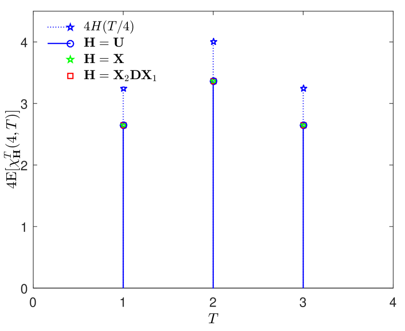
We coin the limit (47 binary entropy loss as it only involves the binary entropy function evaluated at the aspect ratios ϕ italic-ϕ \phi β / ϕ 𝛽 italic-ϕ \beta/\phi β = ϕ 𝛽 italic-ϕ \beta=\phi H ( ϕ ) / ϕ 𝐻 italic-ϕ italic-ϕ H(\phi)/\phi
V-A 5
We show a symmetry property of the universal rate loss in the case when the end system after (completion of the antenna removal) is square, i.e. β = ϕ 𝛽 italic-ϕ \beta=\phi 3 × 2 3 2 3\times 2 3 × 1 3 1 3\times 1 3 × 1 → 1 × 1 → 3 1 1 1 3\times 1\to 1\times 1 3 × 2 → 2 × 2 → 3 2 2 2 3\times 2\to 2\times 2 1 3 H ( 1 / 3 ) = 3 H ( 2 / 3 ) = 2.75 3 𝐻 1 3 3 𝐻 2 3 2.75 3H(1/3)=3H(2/3)=2.75
Note that the expressions T χ T ( R , T ) 𝑇 superscript 𝜒 𝑇 𝑅 𝑇 T\chi^{T}(R,T) T ′ χ T ′ ( R , T ′ ) superscript 𝑇 ′ superscript 𝜒 superscript 𝑇 ′ 𝑅 superscript 𝑇 ′ T^{\prime}\chi^{T^{\prime}}(R,T^{\prime}) R × T → T × T → 𝑅 𝑇 𝑇 𝑇 R\times T\to T\times T R × T ′ → T ′ × T ′ → 𝑅 superscript 𝑇 ′ superscript 𝑇 ′ superscript 𝑇 ′ R\times T^{\prime}\to T^{\prime}\times T^{\prime} T × ( R − T ) 𝑇 𝑅 𝑇 T\times(R-T) R 𝑅 R T χ T ( R , T ) 𝑇 superscript 𝜒 𝑇 𝑅 𝑇 T\chi^{T}(R,T) T 𝑇 T T = R / 2 𝑇 𝑅 2 T=R/2
Since χ ϕ R ( R , β R ) ≤ χ ϕ R ( R , ϕ R ) superscript 𝜒 italic-ϕ 𝑅 𝑅 𝛽 𝑅 superscript 𝜒 italic-ϕ 𝑅 𝑅 italic-ϕ 𝑅 \chi^{\phi R}(R,\beta R)\leq\chi^{\phi R}(R,\phi R) 49 ϕ = β = 1 / 2 italic-ϕ 𝛽 1 2 \phi=\beta=1/2
V-B Case (ii) – Removing transmit antennas
We remove a fraction ( 1 − β ) 1 𝛽 (1-\beta) 8 14 β ≥ 1 / ϕ 𝛽 1 italic-ϕ \beta\geq 1/\phi ϕ = T / R italic-ϕ 𝑇 𝑅 \phi=T/R min ( β T , R ) = T 𝛽 𝑇 𝑅 𝑇 \min(\beta T,R)=T T ℐ ( γ ; F 𝑯 T ) − β T ℐ ( γ ; F 𝑯 𝑷 β † β T ) 𝑇 ℐ 𝛾 subscript superscript F 𝑇 𝑯
𝛽 𝑇 ℐ 𝛾 subscript superscript F 𝛽 𝑇 superscript subscript 𝑯 𝑷 𝛽 †
T\mathcal{I}(\gamma;{\rm F}^{T}_{{\mathchoice{\mbox{\boldmath$\displaystyle H$}}{\mbox{\boldmath$\textstyle H$}}{\mbox{\boldmath$\scriptstyle H$}}{\mbox{\boldmath$\scriptscriptstyle H$}}}})-\beta T\mathcal{I}(\gamma;{\rm F}^{\beta T}_{{\mathchoice{\mbox{\boldmath$\displaystyle H$}}{\mbox{\boldmath$\textstyle H$}}{\mbox{\boldmath$\scriptstyle H$}}{\mbox{\boldmath$\scriptscriptstyle H$}}}{\mathchoice{\mbox{\boldmath$\displaystyle P$}}{\mbox{\boldmath$\textstyle P$}}{\mbox{\boldmath$\scriptstyle P$}}{\mbox{\boldmath$\scriptscriptstyle P$}}}_{\beta}^{\dagger}})
ℐ ( γ ; F 𝑯 T ) − β ℐ ( γ ; F 𝑯 𝑷 β † β T ) . ℐ 𝛾 subscript superscript F 𝑇 𝑯
𝛽 ℐ 𝛾 subscript superscript F 𝛽 𝑇 superscript subscript 𝑯 𝑷 𝛽 †
\mathcal{I}(\gamma;{\rm F}^{T}_{{\mathchoice{\mbox{\boldmath$\displaystyle H$}}{\mbox{\boldmath$\textstyle H$}}{\mbox{\boldmath$\scriptstyle H$}}{\mbox{\boldmath$\scriptscriptstyle H$}}}})-{\beta}\mathcal{I}(\gamma;{\rm F}^{\beta T}_{{\mathchoice{\mbox{\boldmath$\displaystyle H$}}{\mbox{\boldmath$\textstyle H$}}{\mbox{\boldmath$\scriptstyle H$}}{\mbox{\boldmath$\scriptscriptstyle H$}}}{\mathchoice{\mbox{\boldmath$\displaystyle P$}}{\mbox{\boldmath$\textstyle P$}}{\mbox{\boldmath$\scriptstyle P$}}{\mbox{\boldmath$\scriptscriptstyle P$}}}_{\beta}^{\dagger}}). (51)
Let 𝑯 𝑯 \textstyle H 𝑯 𝑷 β † superscript subscript 𝑯 𝑷 𝛽 † {\mathchoice{\mbox{\boldmath$\displaystyle H$}}{\mbox{\boldmath$\textstyle H$}}{\mbox{\boldmath$\scriptstyle H$}}{\mbox{\boldmath$\scriptscriptstyle H$}}}{\mathchoice{\mbox{\boldmath$\displaystyle P$}}{\mbox{\boldmath$\textstyle P$}}{\mbox{\boldmath$\scriptstyle P$}}{\mbox{\boldmath$\scriptscriptstyle P$}}}_{\beta}^{\dagger}
χ ~ 𝑯 R ( T , β T ) ≜ lim γ → ∞ ℐ ( γ ; F 𝑯 T ) − β ℐ ( γ ; F 𝑯 𝑷 β † β T ) , β ≥ 1 ϕ . formulae-sequence ≜ superscript subscript ~ 𝜒 𝑯 𝑅 𝑇 𝛽 𝑇 subscript → 𝛾 ℐ 𝛾 subscript superscript F 𝑇 𝑯
𝛽 ℐ 𝛾 subscript superscript F 𝛽 𝑇 superscript subscript 𝑯 𝑷 𝛽 †
𝛽 1 italic-ϕ \tilde{\chi}_{{\mathchoice{\mbox{\boldmath$\displaystyle H$}}{\mbox{\boldmath$\textstyle H$}}{\mbox{\boldmath$\scriptstyle H$}}{\mbox{\boldmath$\scriptscriptstyle H$}}}}^{R}(T,\beta T)\triangleq\lim_{\gamma\to\infty}\mathcal{I}(\gamma;{\rm F}^{T}_{{\mathchoice{\mbox{\boldmath$\displaystyle H$}}{\mbox{\boldmath$\textstyle H$}}{\mbox{\boldmath$\scriptstyle H$}}{\mbox{\boldmath$\scriptscriptstyle H$}}}})-\beta\mathcal{I}(\gamma;{\rm F}^{\beta T}_{{\mathchoice{\mbox{\boldmath$\displaystyle H$}}{\mbox{\boldmath$\textstyle H$}}{\mbox{\boldmath$\scriptstyle H$}}{\mbox{\boldmath$\scriptscriptstyle H$}}}{\mathchoice{\mbox{\boldmath$\displaystyle P$}}{\mbox{\boldmath$\textstyle P$}}{\mbox{\boldmath$\scriptstyle P$}}{\mbox{\boldmath$\scriptscriptstyle P$}}}_{\beta}^{\dagger}})\ ,\quad\beta\geq\frac{1}{\phi}. (52)
Again the full rank assumption is important here. Otherwise the difference (52 γ → ∞ → 𝛾 \gamma\to\infty
Corollary 2
Let 𝐇 𝐇 \textstyle H 𝐇 𝐏 β † superscript subscript 𝐇 𝐏 𝛽 † {\mathchoice{\mbox{\boldmath$\displaystyle H$}}{\mbox{\boldmath$\textstyle H$}}{\mbox{\boldmath$\scriptstyle H$}}{\mbox{\boldmath$\scriptscriptstyle H$}}}{\mathchoice{\mbox{\boldmath$\displaystyle P$}}{\mbox{\boldmath$\textstyle P$}}{\mbox{\boldmath$\scriptstyle P$}}{\mbox{\boldmath$\scriptscriptstyle P$}}}_{\beta}^{\dagger}
χ ~ 𝑯 R ( T , β T ) = − 1 T log 2 det 𝑷 1 ϕ 𝐑 𝐏 β † 𝑷 β 𝑹 † 𝑷 1 ϕ † superscript subscript ~ 𝜒 𝑯 𝑅 𝑇 𝛽 𝑇 1 𝑇 subscript 2 subscript 𝑷 1 italic-ϕ superscript subscript 𝐑 𝐏 𝛽 † subscript 𝑷 𝛽 superscript 𝑹 † superscript subscript 𝑷 1 italic-ϕ † \tilde{\chi}_{{\mathchoice{\mbox{\boldmath$\displaystyle H$}}{\mbox{\boldmath$\textstyle H$}}{\mbox{\boldmath$\scriptstyle H$}}{\mbox{\boldmath$\scriptscriptstyle H$}}}}^{R}(T,\beta T)=-\frac{1}{T}\log_{2}\det{\mathchoice{\mbox{\boldmath$\displaystyle P$}}{\mbox{\boldmath$\textstyle P$}}{\mbox{\boldmath$\scriptstyle P$}}{\mbox{\boldmath$\scriptscriptstyle P$}}}_{\frac{1}{\phi}}{\mathchoice{\mbox{\boldmath$\displaystyle R$}}{\mbox{\boldmath$\textstyle R$}}{\mbox{\boldmath$\scriptstyle R$}}{\mbox{\boldmath$\scriptscriptstyle R$}}}{\mathchoice{\mbox{\boldmath$\displaystyle P$}}{\mbox{\boldmath$\textstyle P$}}{\mbox{\boldmath$\scriptstyle P$}}{\mbox{\boldmath$\scriptscriptstyle P$}}}_{\beta}^{\dagger}{\mathchoice{\mbox{\boldmath$\displaystyle P$}}{\mbox{\boldmath$\textstyle P$}}{\mbox{\boldmath$\scriptstyle P$}}{\mbox{\boldmath$\scriptscriptstyle P$}}}_{\beta}{\mathchoice{\mbox{\boldmath$\displaystyle R$}}{\mbox{\boldmath$\textstyle R$}}{\mbox{\boldmath$\scriptstyle R$}}{\mbox{\boldmath$\scriptscriptstyle R$}}}^{\dagger}{\mathchoice{\mbox{\boldmath$\displaystyle P$}}{\mbox{\boldmath$\textstyle P$}}{\mbox{\boldmath$\scriptstyle P$}}{\mbox{\boldmath$\scriptscriptstyle P$}}}_{\frac{1}{\phi}}^{\dagger} (53)
where 𝐑 𝐑 \textstyle R T × T 𝑇 𝑇 T\times T 𝐇 𝐇 \textstyle H 41
Note that the right-hand side in (53 ϕ italic-ϕ \phi ϕ − 1 superscript italic-ϕ 1 \phi^{-1} 47
β ℐ ( γ ; F 𝑯 𝑷 β † β T ) = 1 ϕ ℐ ( γ ; F 𝑷 β 𝑯 † R ) . 𝛽 ℐ 𝛾 superscript subscript F superscript subscript 𝑯 𝑷 𝛽 † 𝛽 𝑇
1 italic-ϕ ℐ 𝛾 superscript subscript F subscript 𝑷 𝛽 superscript 𝑯 † 𝑅
\beta\mathcal{I}(\gamma;{\rm F}_{{\mathchoice{\mbox{\boldmath$\displaystyle H$}}{\mbox{\boldmath$\textstyle H$}}{\mbox{\boldmath$\scriptstyle H$}}{\mbox{\boldmath$\scriptscriptstyle H$}}}{\mathchoice{\mbox{\boldmath$\displaystyle P$}}{\mbox{\boldmath$\textstyle P$}}{\mbox{\boldmath$\scriptstyle P$}}{\mbox{\boldmath$\scriptscriptstyle P$}}}_{\beta}^{\dagger}}^{\beta T})=\frac{1}{\phi}\mathcal{I}(\gamma;{\rm F}_{{\mathchoice{\mbox{\boldmath$\displaystyle P$}}{\mbox{\boldmath$\textstyle P$}}{\mbox{\boldmath$\scriptstyle P$}}{\mbox{\boldmath$\scriptscriptstyle P$}}}_{\beta}{\mathchoice{\mbox{\boldmath$\displaystyle H$}}{\mbox{\boldmath$\textstyle H$}}{\mbox{\boldmath$\scriptstyle H$}}{\mbox{\boldmath$\scriptscriptstyle H$}}}^{\dagger}}^{R}). (54)
This substitution is valid for any result that refers to mutual information, e.g. as in Corollary 1 2
V-C The rate loss with antenna power profile
In this subsection we address the rate loss χ 𝑯 T superscript subscript 𝜒 𝑯 𝑇 \chi_{{\mathchoice{\mbox{\boldmath$\displaystyle H$}}{\mbox{\boldmath$\textstyle H$}}{\mbox{\boldmath$\scriptstyle H$}}{\mbox{\boldmath$\scriptscriptstyle H$}}}}^{T}
𝑯 = 𝚲 R 𝑯 ~ 𝚲 T . 𝑯 subscript 𝚲 R subscript 𝑯 ~ 𝚲 T {\mathchoice{\mbox{\boldmath$\displaystyle H$}}{\mbox{\boldmath$\textstyle H$}}{\mbox{\boldmath$\scriptstyle H$}}{\mbox{\boldmath$\scriptscriptstyle H$}}}={{{\mathchoice{\mbox{\boldmath$\displaystyle\Lambda$}}{\mbox{\boldmath$\textstyle\Lambda$}}{\mbox{\boldmath$\scriptstyle\Lambda$}}{\mbox{\boldmath$\scriptscriptstyle\Lambda$}}}_{\rm R}}}{\mathchoice{\mbox{\boldmath$\displaystyle\tilde{H}$}}{\mbox{\boldmath$\textstyle\tilde{H}$}}{\mbox{\boldmath$\scriptstyle\tilde{H}$}}{\mbox{\boldmath$\scriptscriptstyle\tilde{H}$}}}{{\mathchoice{\mbox{\boldmath$\displaystyle\Lambda$}}{\mbox{\boldmath$\textstyle\Lambda$}}{\mbox{\boldmath$\scriptstyle\Lambda$}}{\mbox{\boldmath$\scriptscriptstyle\Lambda$}}}_{\rm T}}. (55)
Here, the matrices 𝚲 R ∈ ℂ R × R subscript 𝚲 R superscript ℂ 𝑅 𝑅 {\mathchoice{\mbox{\boldmath$\displaystyle\Lambda$}}{\mbox{\boldmath$\textstyle\Lambda$}}{\mbox{\boldmath$\scriptstyle\Lambda$}}{\mbox{\boldmath$\scriptscriptstyle\Lambda$}}}_{\rm R}\in\mathbb{C}^{R\times R} 𝚲 T ∈ ℂ T × T subscript 𝚲 T superscript ℂ 𝑇 𝑇 {\mathchoice{\mbox{\boldmath$\displaystyle\Lambda$}}{\mbox{\boldmath$\textstyle\Lambda$}}{\mbox{\boldmath$\scriptstyle\Lambda$}}{\mbox{\boldmath$\scriptscriptstyle\Lambda$}}}_{\rm T}\in\mathbb{C}^{T\times T} 𝚲 R subscript 𝚲 R {\mathchoice{\mbox{\boldmath$\displaystyle\Lambda$}}{\mbox{\boldmath$\textstyle\Lambda$}}{\mbox{\boldmath$\scriptstyle\Lambda$}}{\mbox{\boldmath$\scriptscriptstyle\Lambda$}}}_{\rm R} 𝚲 T subscript 𝚲 T {\mathchoice{\mbox{\boldmath$\displaystyle\Lambda$}}{\mbox{\boldmath$\textstyle\Lambda$}}{\mbox{\boldmath$\scriptstyle\Lambda$}}{\mbox{\boldmath$\scriptscriptstyle\Lambda$}}}_{\rm T}
We generalize Theorem 2 55 H
χ 𝑯 T ( R , β R ) = 1 T log 2 det 𝑷 ϕ 𝑳 ~ † Θ 1 𝑳 ~ 𝑷 ϕ † det 𝑷 ϕ 𝑳 ~ † Θ β 𝑳 ~ 𝑷 ϕ † superscript subscript 𝜒 𝑯 𝑇 𝑅 𝛽 𝑅 1 𝑇 subscript 2 subscript 𝑷 italic-ϕ superscript bold-~ 𝑳 † subscript Θ 1 superscript subscript 𝑳 ~ 𝑷 italic-ϕ † subscript 𝑷 italic-ϕ superscript bold-~ 𝑳 † subscript Θ 𝛽 superscript subscript 𝑳 ~ 𝑷 italic-ϕ † \chi_{{\mathchoice{\mbox{\boldmath$\displaystyle H$}}{\mbox{\boldmath$\textstyle H$}}{\mbox{\boldmath$\scriptstyle H$}}{\mbox{\boldmath$\scriptscriptstyle H$}}}}^{T}(R,\beta R)=\frac{1}{T}\log_{2}\frac{\det{\mathchoice{\mbox{\boldmath$\displaystyle P$}}{\mbox{\boldmath$\textstyle P$}}{\mbox{\boldmath$\scriptstyle P$}}{\mbox{\boldmath$\scriptscriptstyle P$}}}_{\phi}{\mathchoice{\mbox{\boldmath$\displaystyle\tilde{L}$}}{\mbox{\boldmath$\textstyle\tilde{L}$}}{\mbox{\boldmath$\scriptstyle\tilde{L}$}}{\mbox{\boldmath$\scriptscriptstyle\tilde{L}$}}}^{\dagger}\Theta_{1}{\mathchoice{\mbox{\boldmath$\displaystyle\tilde{L}$}}{\mbox{\boldmath$\textstyle\tilde{L}$}}{\mbox{\boldmath$\scriptstyle\tilde{L}$}}{\mbox{\boldmath$\scriptscriptstyle\tilde{L}$}}}{\mathchoice{\mbox{\boldmath$\displaystyle P$}}{\mbox{\boldmath$\textstyle P$}}{\mbox{\boldmath$\scriptstyle P$}}{\mbox{\boldmath$\scriptscriptstyle P$}}}_{\phi}^{\dagger}}{\det{\mathchoice{\mbox{\boldmath$\displaystyle P$}}{\mbox{\boldmath$\textstyle P$}}{\mbox{\boldmath$\scriptstyle P$}}{\mbox{\boldmath$\scriptscriptstyle P$}}}_{\phi}{\mathchoice{\mbox{\boldmath$\displaystyle\tilde{L}$}}{\mbox{\boldmath$\textstyle\tilde{L}$}}{\mbox{\boldmath$\scriptstyle\tilde{L}$}}{\mbox{\boldmath$\scriptscriptstyle\tilde{L}$}}}^{\dagger}\Theta_{\beta}{\mathchoice{\mbox{\boldmath$\displaystyle\tilde{L}$}}{\mbox{\boldmath$\textstyle\tilde{L}$}}{\mbox{\boldmath$\scriptstyle\tilde{L}$}}{\mbox{\boldmath$\scriptscriptstyle\tilde{L}$}}}{\mathchoice{\mbox{\boldmath$\displaystyle P$}}{\mbox{\boldmath$\textstyle P$}}{\mbox{\boldmath$\scriptstyle P$}}{\mbox{\boldmath$\scriptscriptstyle P$}}}_{\phi}^{\dagger}} (56)
where Θ β ≜ 𝚲 R † 𝑷 β † 𝑷 β 𝚲 R ≜ subscript Θ 𝛽 superscript subscript 𝚲 R † superscript subscript 𝑷 𝛽 † subscript 𝑷 𝛽 subscript 𝚲 R \Theta_{\beta}\triangleq{{{{\mathchoice{\mbox{\boldmath$\displaystyle\Lambda$}}{\mbox{\boldmath$\textstyle\Lambda$}}{\mbox{\boldmath$\scriptstyle\Lambda$}}{\mbox{\boldmath$\scriptscriptstyle\Lambda$}}}_{\rm R}}}}^{\dagger}{\mathchoice{\mbox{\boldmath$\displaystyle P$}}{\mbox{\boldmath$\textstyle P$}}{\mbox{\boldmath$\scriptstyle P$}}{\mbox{\boldmath$\scriptscriptstyle P$}}}_{\beta}^{\dagger}{\mathchoice{\mbox{\boldmath$\displaystyle P$}}{\mbox{\boldmath$\textstyle P$}}{\mbox{\boldmath$\scriptstyle P$}}{\mbox{\boldmath$\scriptscriptstyle P$}}}_{\beta}{{{{\mathchoice{\mbox{\boldmath$\displaystyle\Lambda$}}{\mbox{\boldmath$\textstyle\Lambda$}}{\mbox{\boldmath$\scriptstyle\Lambda$}}{\mbox{\boldmath$\scriptscriptstyle\Lambda$}}}_{\rm R}}}} β ≤ 1 𝛽 1 \beta\leq 1 𝑳 ~ bold-~ 𝑳 \textstyle\tilde{L} R × R 𝑅 𝑅 R\times R 𝑯 ~ bold-~ 𝑯 \textstyle\tilde{H} 41 𝑯 ~ bold-~ 𝑯 \textstyle\tilde{H} E [ χ 𝑯 T ( R , β R ) ] E delimited-[] superscript subscript 𝜒 𝑯 𝑇 𝑅 𝛽 𝑅 {\rm E}[\chi_{{\mathchoice{\mbox{\boldmath$\displaystyle H$}}{\mbox{\boldmath$\textstyle H$}}{\mbox{\boldmath$\scriptstyle H$}}{\mbox{\boldmath$\scriptscriptstyle H$}}}}^{T}(R,\beta R)] 𝑯 ~ † 𝑯 ~ superscript bold-~ 𝑯 † bold-~ 𝑯 {\mathchoice{\mbox{\boldmath$\displaystyle\tilde{H}$}}{\mbox{\boldmath$\textstyle\tilde{H}$}}{\mbox{\boldmath$\scriptstyle\tilde{H}$}}{\mbox{\boldmath$\scriptscriptstyle\tilde{H}$}}}^{\dagger}{\mathchoice{\mbox{\boldmath$\displaystyle\tilde{H}$}}{\mbox{\boldmath$\textstyle\tilde{H}$}}{\mbox{\boldmath$\scriptstyle\tilde{H}$}}{\mbox{\boldmath$\scriptscriptstyle\tilde{H}$}}} 𝑳 ~ bold-~ 𝑳 \textstyle\tilde{L} 56
Corollary 3
Let 𝐇 𝐇 \textstyle H 55 𝐇 ~ † 𝐇 ~ superscript bold-~ 𝐇 † bold-~ 𝐇 {\mathchoice{\mbox{\boldmath$\displaystyle\tilde{H}$}}{\mbox{\boldmath$\textstyle\tilde{H}$}}{\mbox{\boldmath$\scriptstyle\tilde{H}$}}{\mbox{\boldmath$\scriptscriptstyle\tilde{H}$}}}^{\dagger}{\mathchoice{\mbox{\boldmath$\displaystyle\tilde{H}$}}{\mbox{\boldmath$\textstyle\tilde{H}$}}{\mbox{\boldmath$\scriptstyle\tilde{H}$}}{\mbox{\boldmath$\scriptscriptstyle\tilde{H}$}}} 𝐗 β ≜ 𝐏 β 𝐗 ≜ subscript 𝐗 𝛽 subscript 𝐏 𝛽 𝐗 {\mathchoice{\mbox{\boldmath$\displaystyle X$}}{\mbox{\boldmath$\textstyle X$}}{\mbox{\boldmath$\scriptstyle X$}}{\mbox{\boldmath$\scriptscriptstyle X$}}}_{\beta}\triangleq{\mathchoice{\mbox{\boldmath$\displaystyle P$}}{\mbox{\boldmath$\textstyle P$}}{\mbox{\boldmath$\scriptstyle P$}}{\mbox{\boldmath$\scriptscriptstyle P$}}}_{\beta}{\mathchoice{\mbox{\boldmath$\displaystyle X$}}{\mbox{\boldmath$\textstyle X$}}{\mbox{\boldmath$\scriptstyle X$}}{\mbox{\boldmath$\scriptscriptstyle X$}}} 𝐗 𝐗 \textstyle X R × T 𝑅 𝑇 R\times T 𝐃 β subscript 𝐃 𝛽 {\mathchoice{\mbox{\boldmath$\displaystyle D$}}{\mbox{\boldmath$\textstyle D$}}{\mbox{\boldmath$\scriptstyle D$}}{\mbox{\boldmath$\scriptscriptstyle D$}}}_{\beta} β R × β R 𝛽 𝑅 𝛽 𝑅 \beta R\times\beta R Θ β ≜ 𝚲 R † 𝐏 β † 𝐏 β 𝚲 R ≜ subscript Θ 𝛽 superscript subscript 𝚲 R † superscript subscript 𝐏 𝛽 † subscript 𝐏 𝛽 subscript 𝚲 R \Theta_{\beta}\triangleq{{{{\mathchoice{\mbox{\boldmath$\displaystyle\Lambda$}}{\mbox{\boldmath$\textstyle\Lambda$}}{\mbox{\boldmath$\scriptstyle\Lambda$}}{\mbox{\boldmath$\scriptscriptstyle\Lambda$}}}_{\rm R}}}}^{\dagger}{\mathchoice{\mbox{\boldmath$\displaystyle P$}}{\mbox{\boldmath$\textstyle P$}}{\mbox{\boldmath$\scriptstyle P$}}{\mbox{\boldmath$\scriptscriptstyle P$}}}_{\beta}^{\dagger}{\mathchoice{\mbox{\boldmath$\displaystyle P$}}{\mbox{\boldmath$\textstyle P$}}{\mbox{\boldmath$\scriptstyle P$}}{\mbox{\boldmath$\scriptscriptstyle P$}}}_{\beta}{{{{\mathchoice{\mbox{\boldmath$\displaystyle\Lambda$}}{\mbox{\boldmath$\textstyle\Lambda$}}{\mbox{\boldmath$\scriptstyle\Lambda$}}{\mbox{\boldmath$\scriptscriptstyle\Lambda$}}}_{\rm R}}}}
E [ χ 𝑯 T ( R , β R ) ] = 1 T E [ log 2 det 𝑿 1 † 𝑫 1 𝑿 1 det 𝑿 β † 𝑫 β 𝑿 β ] . E delimited-[] superscript subscript 𝜒 𝑯 𝑇 𝑅 𝛽 𝑅 1 𝑇 E delimited-[] subscript 2 superscript subscript 𝑿 1 † subscript 𝑫 1 subscript 𝑿 1 superscript subscript 𝑿 𝛽 † subscript 𝑫 𝛽 subscript 𝑿 𝛽 {\rm E}[\chi_{{\mathchoice{\mbox{\boldmath$\displaystyle H$}}{\mbox{\boldmath$\textstyle H$}}{\mbox{\boldmath$\scriptstyle H$}}{\mbox{\boldmath$\scriptscriptstyle H$}}}}^{T}(R,\beta R)]=\frac{1}{T}{\rm E}\left[\log_{2}\frac{\det{\mathchoice{\mbox{\boldmath$\displaystyle X$}}{\mbox{\boldmath$\textstyle X$}}{\mbox{\boldmath$\scriptstyle X$}}{\mbox{\boldmath$\scriptscriptstyle X$}}}_{1}^{\dagger}{\mathchoice{\mbox{\boldmath$\displaystyle D$}}{\mbox{\boldmath$\textstyle D$}}{\mbox{\boldmath$\scriptstyle D$}}{\mbox{\boldmath$\scriptscriptstyle D$}}}_{1}{\mathchoice{\mbox{\boldmath$\displaystyle X$}}{\mbox{\boldmath$\textstyle X$}}{\mbox{\boldmath$\scriptstyle X$}}{\mbox{\boldmath$\scriptscriptstyle X$}}}_{1}}{\det{\mathchoice{\mbox{\boldmath$\displaystyle X$}}{\mbox{\boldmath$\textstyle X$}}{\mbox{\boldmath$\scriptstyle X$}}{\mbox{\boldmath$\scriptscriptstyle X$}}}_{\beta}^{\dagger}{\mathchoice{\mbox{\boldmath$\displaystyle D$}}{\mbox{\boldmath$\textstyle D$}}{\mbox{\boldmath$\scriptstyle D$}}{\mbox{\boldmath$\scriptscriptstyle D$}}}_{\beta}{\mathchoice{\mbox{\boldmath$\displaystyle X$}}{\mbox{\boldmath$\textstyle X$}}{\mbox{\boldmath$\scriptstyle X$}}{\mbox{\boldmath$\scriptscriptstyle X$}}}_{\beta}}\right]. (57)
The expectation in (57
Lemma 1
[ 5 , Lemma 2]
Let 𝐗 𝐗 \textstyle X n × m 𝑛 𝑚 n\times m n > m 𝑛 𝑚 n>m 𝐃 𝐃 \textstyle D n × n 𝑛 𝑛 n\times n j 𝑗 j λ j subscript 𝜆 𝑗 \lambda_{j} 𝛀 𝛀 \textstyle\Omega n × n 𝑛 𝑛 n\times n ( 𝛀 ) i j = λ i j − 1 subscript 𝛀 𝑖 𝑗 superscript subscript 𝜆 𝑖 𝑗 1 ({\mathchoice{\mbox{\boldmath$\displaystyle\Omega$}}{\mbox{\boldmath$\textstyle\Omega$}}{\mbox{\boldmath$\scriptstyle\Omega$}}{\mbox{\boldmath$\scriptscriptstyle\Omega$}}})_{ij}=\lambda_{i}^{j-1} 𝚪 𝚪 \textstyle\Gamma ( n − m ) × ( n − m ) 𝑛 𝑚 𝑛 𝑚 (n-m)\times(n-m) 𝛀 𝛀 \textstyle\Omega
E [ ln det 𝑿 † 𝐃 𝐗 ] = det 𝚪 det 𝛀 ∑ i = 1 m det 𝚿 i E delimited-[] superscript 𝑿 † 𝐃 𝐗 𝚪 𝛀 superscript subscript 𝑖 1 𝑚 subscript 𝚿 𝑖 {\rm E}[\ln\det{\mathchoice{\mbox{\boldmath$\displaystyle X$}}{\mbox{\boldmath$\textstyle X$}}{\mbox{\boldmath$\scriptstyle X$}}{\mbox{\boldmath$\scriptscriptstyle X$}}}^{\dagger}{\mathchoice{\mbox{\boldmath$\displaystyle D$}}{\mbox{\boldmath$\textstyle D$}}{\mbox{\boldmath$\scriptstyle D$}}{\mbox{\boldmath$\scriptscriptstyle D$}}}{\mathchoice{\mbox{\boldmath$\displaystyle X$}}{\mbox{\boldmath$\textstyle X$}}{\mbox{\boldmath$\scriptstyle X$}}{\mbox{\boldmath$\scriptscriptstyle X$}}}]=\frac{\det{\mathchoice{\mbox{\boldmath$\displaystyle\Gamma$}}{\mbox{\boldmath$\textstyle\Gamma$}}{\mbox{\boldmath$\scriptstyle\Gamma$}}{\mbox{\boldmath$\scriptscriptstyle\Gamma$}}}}{\det{\mathchoice{\mbox{\boldmath$\displaystyle\Omega$}}{\mbox{\boldmath$\textstyle\Omega$}}{\mbox{\boldmath$\scriptstyle\Omega$}}{\mbox{\boldmath$\scriptscriptstyle\Omega$}}}}\sum_{i=1}^{m}\det{\mathchoice{\mbox{\boldmath$\displaystyle\Psi$}}{\mbox{\boldmath$\textstyle\Psi$}}{\mbox{\boldmath$\scriptstyle\Psi$}}{\mbox{\boldmath$\scriptscriptstyle\Psi$}}}_{i} (58)
where 𝚿 i subscript 𝚿 𝑖 {\mathchoice{\mbox{\boldmath$\displaystyle\Psi$}}{\mbox{\boldmath$\textstyle\Psi$}}{\mbox{\boldmath$\scriptstyle\Psi$}}{\mbox{\boldmath$\scriptscriptstyle\Psi$}}}_{i} m × m 𝑚 𝑚 m\times m
( 𝚿 i ) k , l = subscript subscript 𝚿 𝑖 𝑘 𝑙
absent \displaystyle({\mathchoice{\mbox{\boldmath$\displaystyle\Psi$}}{\mbox{\boldmath$\textstyle\Psi$}}{\mbox{\boldmath$\scriptstyle\Psi$}}{\mbox{\boldmath$\scriptscriptstyle\Psi$}}}_{i})_{k,l}= ν n − m + k λ n − m + k n − m − 1 + l subscript 𝜈 𝑛 𝑚 𝑘 superscript subscript 𝜆 𝑛 𝑚 𝑘 𝑛 𝑚 1 𝑙 \displaystyle\nu_{n-m+k}\lambda_{n-m+k}^{n-m-1+l}
− ∑ d = 1 , q = 1 n − m ν q ( 𝚪 − 1 ) d , q d − 1 λ n − m + k d − 1 λ q n − m − 1 + 1 . superscript subscript formulae-sequence 𝑑 1 𝑞 1 𝑛 𝑚 subscript 𝜈 𝑞 superscript subscript superscript 𝚪 1 𝑑 𝑞
𝑑 1 superscript subscript 𝜆 𝑛 𝑚 𝑘 𝑑 1 superscript subscript 𝜆 𝑞 𝑛 𝑚 1 1 \displaystyle-\sum_{d=1,q=1}^{n-m}\nu_{q}({\mathchoice{\mbox{\boldmath$\displaystyle\Gamma$}}{\mbox{\boldmath$\textstyle\Gamma$}}{\mbox{\boldmath$\scriptstyle\Gamma$}}{\mbox{\boldmath$\scriptscriptstyle\Gamma$}}}^{-1})_{d,q}^{d-1}\lambda_{n-m+k}^{d-1}\lambda_{q}^{n-m-1+1}. (59)
In this expression, ν q = ψ ( l ) + ln λ q subscript 𝜈 𝑞 𝜓 𝑙 subscript 𝜆 𝑞 \nu_{q}=\psi(l)+\ln\lambda_{q} l = i 𝑙 𝑖 l=i ν q = 1 subscript 𝜈 𝑞 1 \nu_{q}=1 ψ ( ⋅ ) 𝜓 ⋅ \psi(\cdot)
V-D Further discussions based on numerical results
As a warm up example, consider a 4 × 2 4 2 4\times 2 4 χ 2 ( 4 , 2 ) = 3.37 4 superscript 𝜒 2 4 2 3.37 4\chi^{2}(4,2)=3.37 47 4 H ( 2 / 4 ) = 4 4 𝐻 2 4 4 4H(2/4)=4
Figure 1: Ergodic mutual information (continuous lines) and ergodic multiplexing rate (dashed lines) versus the SNR of a zero-mean iid complex Gaussian MIMO channel with T = 2 𝑇 2 T=2 R = 4 𝑅 4 R=4 R = 2 𝑅 2 R=2
Note also that 4 χ 2 ( 4 , 2 ) 4 superscript 𝜒 2 4 2 4\chi^{2}(4,2)
Figure 2: The maximal ergodic mutual information loss over the SNR range: The entries of 𝑿 ∈ ℂ 4 × T 𝑿 superscript ℂ 4 𝑇 {\mathchoice{\mbox{\boldmath$\displaystyle X$}}{\mbox{\boldmath$\textstyle X$}}{\mbox{\boldmath$\scriptstyle X$}}{\mbox{\boldmath$\scriptscriptstyle X$}}}\in\mathbb{C}^{4\times T} 𝑿 1 ∈ ℂ S = 4 × T subscript 𝑿 1 superscript ℂ 𝑆 4 𝑇 {\mathchoice{\mbox{\boldmath$\displaystyle X$}}{\mbox{\boldmath$\textstyle X$}}{\mbox{\boldmath$\scriptstyle X$}}{\mbox{\boldmath$\scriptscriptstyle X$}}}_{1}\in\mathbb{C}^{S=4\times T} 𝑿 2 ∈ ℂ 4 × S = 4 subscript 𝑿 2 superscript ℂ 4 𝑆 4 {\mathchoice{\mbox{\boldmath$\displaystyle X$}}{\mbox{\boldmath$\textstyle X$}}{\mbox{\boldmath$\scriptstyle X$}}{\mbox{\boldmath$\scriptscriptstyle X$}}}_{2}\in\mathbb{C}^{4\times S=4} 𝑼 ∈ ℂ 4 × T 𝑼 superscript ℂ 4 𝑇 {\mathchoice{\mbox{\boldmath$\displaystyle U$}}{\mbox{\boldmath$\textstyle U$}}{\mbox{\boldmath$\scriptstyle U$}}{\mbox{\boldmath$\scriptscriptstyle U$}}}\in\mathbb{C}^{4\times T} 4 × T 4 𝑇 4\times T S × S 𝑆 𝑆 S\times S 𝑫 𝑫 \textstyle D
the universal rate loss and the tightness of the approximation provided by the binary entropy loss, i.e. R H ( T / R ) 𝑅 𝐻 𝑇 𝑅 RH(T/R) 𝑯 = 𝑼 𝚲 𝑯 𝑼 𝚲 {\mathchoice{\mbox{\boldmath$\displaystyle H$}}{\mbox{\boldmath$\textstyle H$}}{\mbox{\boldmath$\scriptstyle H$}}{\mbox{\boldmath$\scriptscriptstyle H$}}}={\mathchoice{\mbox{\boldmath$\displaystyle U$}}{\mbox{\boldmath$\textstyle U$}}{\mbox{\boldmath$\scriptstyle U$}}{\mbox{\boldmath$\scriptscriptstyle U$}}}{{\mathchoice{\mbox{\boldmath$\displaystyle\Lambda$}}{\mbox{\boldmath$\textstyle\Lambda$}}{\mbox{\boldmath$\scriptstyle\Lambda$}}{\mbox{\boldmath$\scriptscriptstyle\Lambda$}}}} 𝑼 ∈ ℂ R × T 𝑼 superscript ℂ 𝑅 𝑇 {\mathchoice{\mbox{\boldmath$\displaystyle U$}}{\mbox{\boldmath$\textstyle U$}}{\mbox{\boldmath$\scriptstyle U$}}{\mbox{\boldmath$\scriptscriptstyle U$}}}\in\mathbb{C}^{R\times T} R × T 𝑅 𝑇 R\times T 𝑼 † 𝑼 = 𝑰 superscript 𝑼 † 𝑼 𝑰 {\mathchoice{\mbox{\boldmath$\displaystyle U$}}{\mbox{\boldmath$\textstyle U$}}{\mbox{\boldmath$\scriptstyle U$}}{\mbox{\boldmath$\scriptscriptstyle U$}}}^{\dagger}{\mathchoice{\mbox{\boldmath$\displaystyle U$}}{\mbox{\boldmath$\textstyle U$}}{\mbox{\boldmath$\scriptstyle U$}}{\mbox{\boldmath$\scriptscriptstyle U$}}}={\mathchoice{\mbox{\boldmath$\displaystyle I$}}{\mbox{\boldmath$\textstyle I$}}{\mbox{\boldmath$\scriptstyle I$}}{\mbox{\boldmath$\scriptscriptstyle I$}}} 𝚲 ∈ ℝ T × T 𝚲 superscript ℝ 𝑇 𝑇 {\mathchoice{\mbox{\boldmath$\displaystyle\Lambda$}}{\mbox{\boldmath$\textstyle\Lambda$}}{\mbox{\boldmath$\scriptstyle\Lambda$}}{\mbox{\boldmath$\scriptscriptstyle\Lambda$}}}\in\mathbb{R}^{T\times T} T ≪ R much-less-than 𝑇 𝑅 T\ll R 𝚲 𝚲 \textstyle\Lambda 𝚲 = 𝐈 𝚲 𝐈 {\mathchoice{\mbox{\boldmath$\displaystyle\Lambda$}}{\mbox{\boldmath$\textstyle\Lambda$}}{\mbox{\boldmath$\scriptstyle\Lambda$}}{\mbox{\boldmath$\scriptscriptstyle\Lambda$}}}={\mathchoice{\mbox{\boldmath$\displaystyle\bf I$}}{\mbox{\boldmath$\textstyle\bf I$}}{\mbox{\boldmath$\scriptstyle\bf I$}}{\mbox{\boldmath$\scriptscriptstyle\bf I$}}} 𝑯 = 𝑿 𝑯 𝑿 {\mathchoice{\mbox{\boldmath$\displaystyle H$}}{\mbox{\boldmath$\textstyle H$}}{\mbox{\boldmath$\scriptstyle H$}}{\mbox{\boldmath$\scriptscriptstyle H$}}}={\mathchoice{\mbox{\boldmath$\displaystyle X$}}{\mbox{\boldmath$\textstyle X$}}{\mbox{\boldmath$\scriptstyle X$}}{\mbox{\boldmath$\scriptscriptstyle X$}}} 𝑿 𝑿 \textstyle X 𝑯 = 𝑿 2 𝑫 𝑿 1 𝑯 subscript 𝑿 2 subscript 𝑫 𝑿 1 {\mathchoice{\mbox{\boldmath$\displaystyle H$}}{\mbox{\boldmath$\textstyle H$}}{\mbox{\boldmath$\scriptstyle H$}}{\mbox{\boldmath$\scriptscriptstyle H$}}}={\mathchoice{\mbox{\boldmath$\displaystyle X$}}{\mbox{\boldmath$\textstyle X$}}{\mbox{\boldmath$\scriptstyle X$}}{\mbox{\boldmath$\scriptscriptstyle X$}}}_{2}{\mathchoice{\mbox{\boldmath$\displaystyle D$}}{\mbox{\boldmath$\textstyle D$}}{\mbox{\boldmath$\scriptstyle D$}}{\mbox{\boldmath$\scriptscriptstyle D$}}}{\mathchoice{\mbox{\boldmath$\displaystyle X$}}{\mbox{\boldmath$\textstyle X$}}{\mbox{\boldmath$\scriptstyle X$}}{\mbox{\boldmath$\scriptscriptstyle X$}}}_{1} 𝑿 1 ∈ ℂ S × T subscript 𝑿 1 superscript ℂ 𝑆 𝑇 {\mathchoice{\mbox{\boldmath$\displaystyle X$}}{\mbox{\boldmath$\textstyle X$}}{\mbox{\boldmath$\scriptstyle X$}}{\mbox{\boldmath$\scriptscriptstyle X$}}}_{1}\in\mathbb{C}^{S\times T} 𝑿 2 ∈ ℂ R × S subscript 𝑿 2 superscript ℂ 𝑅 𝑆 {\mathchoice{\mbox{\boldmath$\displaystyle X$}}{\mbox{\boldmath$\textstyle X$}}{\mbox{\boldmath$\scriptstyle X$}}{\mbox{\boldmath$\scriptscriptstyle X$}}}_{2}\in\mathbb{C}^{R\times S} 𝑫 𝑫 \textstyle D [18 ] . To fulfill the full-rank condition we restrict to the case S ≥ T 𝑆 𝑇 S\geq T
VI Deviation from Linear Growth
In this section we clarify the second misinterpretation underlined in Section 1. Specifically, we analyze the variation of the multiplexing rate when either the number of receive or the number transmit antennas varies while their maximum is kept fixed.
For a channel matrix having orthogonal columns when the number of transmit or receive antennas varies, the linear growth of mutual information is obvious. However, for a channel matrix with e.g. iid entries, a substantial crosstalk arises due to the lack of orthogonality of its columns. The effect of this crosstalk onto mutual information is non-linear in the number of antennas.
The mutual information scales approximately linearly in the minimum of the numbers of transmit and receive antennas. For a tall rectangular channel matrix that becomes wider and wider, the mutual information can only grow approximately linearly until the matrix becomes square. The same holds for a wide rectangular channel matrix growing taller and taller. Therefore, we have to distinguish between two cases: (i) the number of receive antennas is smaller than the number of transmit antennas, i.e. a wide channel matrix, and (ii) the converse of (i), i.e. a tall channel matrix. Since case (ii) can be easily treated by replacing the channel matrix with its conjugate transpose, we restrict our investigations to case (i).
The linear growth cannot continue once the channel matrix has grown square. Thus, it makes sense to constrain the matrix of reference system (8 we assume that the channel matrix 𝐇 𝐇 \textstyle H 8 N × N 𝑁 𝑁 N\times N N = R = T 𝑁 𝑅 𝑇 N=R=T .
The exact mutual information of the (rectangular) system (14 β N × N 𝛽 𝑁 𝑁 \beta N\times N β ≤ 1 𝛽 1 \beta\leq 1
N ℐ ( γ ; F 𝑷 β 𝑯 N ) . 𝑁 ℐ 𝛾 subscript superscript F 𝑁 subscript 𝑷 𝛽 𝑯
N\mathcal{I}(\gamma;{\rm F}^{N}_{{\mathchoice{\mbox{\boldmath$\displaystyle P$}}{\mbox{\boldmath$\textstyle P$}}{\mbox{\boldmath$\scriptstyle P$}}{\mbox{\boldmath$\scriptscriptstyle P$}}}_{\beta}{\mathchoice{\mbox{\boldmath$\displaystyle H$}}{\mbox{\boldmath$\textstyle H$}}{\mbox{\boldmath$\scriptstyle H$}}{\mbox{\boldmath$\scriptscriptstyle H$}}}}). (60)
The mutual information (60
β N ℐ ( γ ; F 𝑯 N ) . 𝛽 𝑁 ℐ 𝛾 subscript superscript F 𝑁 𝑯
\beta N\mathcal{I}(\gamma;{\rm F}^{N}_{{\mathchoice{\mbox{\boldmath$\displaystyle H$}}{\mbox{\boldmath$\textstyle H$}}{\mbox{\boldmath$\scriptstyle H$}}{\mbox{\boldmath$\scriptscriptstyle H$}}}}). (61)
Thus, in the high SNR limit, the deviation from the linear growth normalized to N 𝑁 N
Δ ℒ ( β ; F 𝑯 N ) Δ ℒ 𝛽 subscript superscript F 𝑁 𝑯
\displaystyle\Delta\mathcal{L}(\beta;{\rm F}^{N}_{\mathchoice{\mbox{\boldmath$\displaystyle H$}}{\mbox{\boldmath$\textstyle H$}}{\mbox{\boldmath$\scriptstyle H$}}{\mbox{\boldmath$\scriptscriptstyle H$}}}) ≜ lim γ → ∞ ℐ ( γ ; F 𝑷 β 𝑯 N ) − β ℐ ( γ ; F 𝑯 N ) ≜ absent subscript → 𝛾 ℐ 𝛾 subscript superscript F 𝑁 subscript 𝑷 𝛽 𝑯
𝛽 ℐ 𝛾 subscript superscript F 𝑁 𝑯
\displaystyle\triangleq\lim_{\gamma\to\infty}\mathcal{I}(\gamma;{\rm F}^{N}_{{\mathchoice{\mbox{\boldmath$\displaystyle P$}}{\mbox{\boldmath$\textstyle P$}}{\mbox{\boldmath$\scriptstyle P$}}{\mbox{\boldmath$\scriptscriptstyle P$}}}_{\beta}{\mathchoice{\mbox{\boldmath$\displaystyle H$}}{\mbox{\boldmath$\textstyle H$}}{\mbox{\boldmath$\scriptstyle H$}}{\mbox{\boldmath$\scriptscriptstyle H$}}}})-\beta\mathcal{I}(\gamma;{\rm F}^{N}_{{\mathchoice{\mbox{\boldmath$\displaystyle H$}}{\mbox{\boldmath$\textstyle H$}}{\mbox{\boldmath$\scriptstyle H$}}{\mbox{\boldmath$\scriptscriptstyle H$}}}}) (62)
= ℐ 0 ( γ ; F 𝑷 β 𝑯 N ) − β ℐ 0 ( γ ; F 𝑯 N ) absent subscript ℐ 0 𝛾 subscript superscript F 𝑁 subscript 𝑷 𝛽 𝑯
𝛽 subscript ℐ 0 𝛾 subscript superscript F 𝑁 𝑯
\displaystyle=\mathcal{I}_{0}(\gamma;{\rm F}^{N}_{{\mathchoice{\mbox{\boldmath$\displaystyle P$}}{\mbox{\boldmath$\textstyle P$}}{\mbox{\boldmath$\scriptstyle P$}}{\mbox{\boldmath$\scriptscriptstyle P$}}}_{\beta}{\mathchoice{\mbox{\boldmath$\displaystyle H$}}{\mbox{\boldmath$\textstyle H$}}{\mbox{\boldmath$\scriptstyle H$}}{\mbox{\boldmath$\scriptscriptstyle H$}}}})-\beta\mathcal{I}_{0}(\gamma;{\rm F}^{N}_{{\mathchoice{\mbox{\boldmath$\displaystyle H$}}{\mbox{\boldmath$\textstyle H$}}{\mbox{\boldmath$\scriptstyle H$}}{\mbox{\boldmath$\scriptscriptstyle H$}}}}) (63)
where 𝑯 𝑯 \textstyle H α 𝑯 T = α 𝑷 β 𝑯 T subscript superscript 𝛼 𝑇 𝑯 subscript superscript 𝛼 𝑇 subscript 𝑷 𝛽 𝑯 \alpha^{T}_{{\mathchoice{\mbox{\boldmath$\displaystyle H$}}{\mbox{\boldmath$\textstyle H$}}{\mbox{\boldmath$\scriptstyle H$}}{\mbox{\boldmath$\scriptscriptstyle H$}}}}=\alpha^{T}_{{\mathchoice{\mbox{\boldmath$\displaystyle P$}}{\mbox{\boldmath$\textstyle P$}}{\mbox{\boldmath$\scriptstyle P$}}{\mbox{\boldmath$\scriptscriptstyle P$}}}_{\beta}{\mathchoice{\mbox{\boldmath$\displaystyle H$}}{\mbox{\boldmath$\textstyle H$}}{\mbox{\boldmath$\scriptstyle H$}}{\mbox{\boldmath$\scriptscriptstyle H$}}}} 62 62
Example 3
Let 𝐇 𝐇 \textstyle H
Δ ℒ ( β ; F 𝑯 N ) = 0 . Δ ℒ 𝛽 subscript superscript F 𝑁 𝑯
0 \Delta\mathcal{L}(\beta;{\rm F}^{N}_{\mathchoice{\mbox{\boldmath$\displaystyle H$}}{\mbox{\boldmath$\textstyle H$}}{\mbox{\boldmath$\scriptstyle H$}}{\mbox{\boldmath$\scriptscriptstyle H$}}})=0. (64)
VI-A The large-system limit consideration
The deviation from linear growth (63 χ 𝑯 T superscript subscript 𝜒 𝑯 𝑇 \chi_{{\mathchoice{\mbox{\boldmath$\displaystyle H$}}{\mbox{\boldmath$\textstyle H$}}{\mbox{\boldmath$\scriptstyle H$}}{\mbox{\boldmath$\scriptscriptstyle H$}}}}^{T} 35 β 𝛽 \beta χ 𝑯 T superscript subscript 𝜒 𝑯 𝑇 \chi_{{\mathchoice{\mbox{\boldmath$\displaystyle H$}}{\mbox{\boldmath$\textstyle H$}}{\mbox{\boldmath$\scriptstyle H$}}{\mbox{\boldmath$\scriptscriptstyle H$}}}}^{T} Δ ℒ Δ ℒ \Delta\mathcal{L}
Assumption 1
The channel matrix 𝐇 𝐇 \textstyle H 𝐇 𝐇 † superscript 𝐇 𝐇 † {\mathchoice{\mbox{\boldmath$\displaystyle H$}}{\mbox{\boldmath$\textstyle H$}}{\mbox{\boldmath$\scriptstyle H$}}{\mbox{\boldmath$\scriptscriptstyle H$}}}{\mathchoice{\mbox{\boldmath$\displaystyle H$}}{\mbox{\boldmath$\textstyle H$}}{\mbox{\boldmath$\scriptstyle H$}}{\mbox{\boldmath$\scriptscriptstyle H$}}}^{\dagger} N → ∞ → 𝑁 N\to\infty Δ ℐ ( 1 ; F 𝐇 ) Δ ℐ 1 subscript F 𝐇
\Delta{\mathcal{I}}(1;{\rm F}_{{\mathchoice{\mbox{\boldmath$\displaystyle H$}}{\mbox{\boldmath$\textstyle H$}}{\mbox{\boldmath$\scriptstyle H$}}{\mbox{\boldmath$\scriptscriptstyle H$}}}})
We carry out the analysis on the basis of the LED function F 𝑷 β 𝑯 subscript F subscript 𝑷 𝛽 𝑯 {\rm F}_{{\mathchoice{\mbox{\boldmath$\displaystyle P$}}{\mbox{\boldmath$\textstyle P$}}{\mbox{\boldmath$\scriptstyle P$}}{\mbox{\boldmath$\scriptscriptstyle P$}}}_{\beta}{\mathchoice{\mbox{\boldmath$\displaystyle H$}}{\mbox{\boldmath$\textstyle H$}}{\mbox{\boldmath$\scriptstyle H$}}{\mbox{\boldmath$\scriptscriptstyle H$}}}}
Δ ℒ ( β ; F 𝑯 ) = ℐ 0 ( γ ; F 𝑷 β 𝑯 ) − β ℐ 0 ( γ ; F 𝑯 ) . Δ ℒ 𝛽 subscript F 𝑯
subscript ℐ 0 𝛾 subscript F subscript 𝑷 𝛽 𝑯
𝛽 subscript ℐ 0 𝛾 subscript F 𝑯
\Delta\mathcal{L}(\beta;{\rm F}_{\mathchoice{\mbox{\boldmath$\displaystyle H$}}{\mbox{\boldmath$\textstyle H$}}{\mbox{\boldmath$\scriptstyle H$}}{\mbox{\boldmath$\scriptscriptstyle H$}}})=\mathcal{I}_{0}(\gamma;{\rm F}_{{\mathchoice{\mbox{\boldmath$\displaystyle P$}}{\mbox{\boldmath$\textstyle P$}}{\mbox{\boldmath$\scriptstyle P$}}{\mbox{\boldmath$\scriptscriptstyle P$}}}_{\beta}{\mathchoice{\mbox{\boldmath$\displaystyle H$}}{\mbox{\boldmath$\textstyle H$}}{\mbox{\boldmath$\scriptstyle H$}}{\mbox{\boldmath$\scriptscriptstyle H$}}}})-\beta\mathcal{I}_{0}(\gamma;{\rm F}_{{\mathchoice{\mbox{\boldmath$\displaystyle H$}}{\mbox{\boldmath$\textstyle H$}}{\mbox{\boldmath$\scriptstyle H$}}{\mbox{\boldmath$\scriptscriptstyle H$}}}}). (65)
When we interpret the asymptotic results in the numerical investigations we assume that
lim N → ∞ E [ ℐ 0 ( γ ; F 𝑷 β 𝑯 N ) ] = ℐ 0 ( γ ; F 𝑷 β 𝑯 ) , β ≤ 1 . formulae-sequence subscript → 𝑁 E delimited-[] subscript ℐ 0 𝛾 subscript superscript F 𝑁 subscript 𝑷 𝛽 𝑯
subscript ℐ 0 𝛾 subscript F subscript 𝑷 𝛽 𝑯
𝛽 1 \lim_{N\to\infty}{\rm E}[\mathcal{I}_{0}(\gamma;{\rm F}^{N}_{{\mathchoice{\mbox{\boldmath$\displaystyle P$}}{\mbox{\boldmath$\textstyle P$}}{\mbox{\boldmath$\scriptstyle P$}}{\mbox{\boldmath$\scriptscriptstyle P$}}}_{\beta}{\mathchoice{\mbox{\boldmath$\displaystyle H$}}{\mbox{\boldmath$\textstyle H$}}{\mbox{\boldmath$\scriptstyle H$}}{\mbox{\boldmath$\scriptscriptstyle H$}}}})]=\mathcal{I}_{0}(\gamma;{\rm F}_{{\mathchoice{\mbox{\boldmath$\displaystyle P$}}{\mbox{\boldmath$\textstyle P$}}{\mbox{\boldmath$\scriptstyle P$}}{\mbox{\boldmath$\scriptscriptstyle P$}}}_{\beta}{\mathchoice{\mbox{\boldmath$\displaystyle H$}}{\mbox{\boldmath$\textstyle H$}}{\mbox{\boldmath$\scriptstyle H$}}{\mbox{\boldmath$\scriptscriptstyle H$}}}})\ ,\quad\beta\leq 1. (66)
It is easy to show that the convergence (66 β < 1 𝛽 1 \beta<1 F 𝑯 subscript F 𝑯 {\rm F}_{{\mathchoice{\mbox{\boldmath$\displaystyle H$}}{\mbox{\boldmath$\textstyle H$}}{\mbox{\boldmath$\scriptstyle H$}}{\mbox{\boldmath$\scriptscriptstyle H$}}}} F 𝑷 β 𝑯 subscript F subscript 𝑷 𝛽 𝑯 {\rm F}_{{\mathchoice{\mbox{\boldmath$\displaystyle P$}}{\mbox{\boldmath$\textstyle P$}}{\mbox{\boldmath$\scriptstyle P$}}{\mbox{\boldmath$\scriptscriptstyle P$}}}_{\beta}{\mathchoice{\mbox{\boldmath$\displaystyle H$}}{\mbox{\boldmath$\textstyle H$}}{\mbox{\boldmath$\scriptstyle H$}}{\mbox{\boldmath$\scriptscriptstyle H$}}}} [19 , Corollary 1.14] . Note that a compactly supported probability distribution can be uniquely characterized by its moments. This fact allow us to use the machinery provided in Proposition 1 in Appendix C. Specifically, sup N E [ ∫ x − 1 d F ~ 𝑷 β 𝑯 N ( x ) ] < ∞ subscript supremum 𝑁 E delimited-[] superscript 𝑥 1 differential-d subscript superscript ~ F 𝑁 subscript 𝑷 𝛽 𝑯 𝑥 \sup_{N}{\rm E}[\int x^{-1}{\rm d}\tilde{\rm F}^{N}_{{\mathchoice{\mbox{\boldmath$\displaystyle P$}}{\mbox{\boldmath$\textstyle P$}}{\mbox{\boldmath$\scriptstyle P$}}{\mbox{\boldmath$\scriptscriptstyle P$}}}_{\beta}{\mathchoice{\mbox{\boldmath$\displaystyle H$}}{\mbox{\boldmath$\textstyle H$}}{\mbox{\boldmath$\scriptstyle H$}}{\mbox{\boldmath$\scriptscriptstyle H$}}}}(x)]<\infty 66 β < 1 𝛽 1 \beta<1
∫ 1 x d F ~ 𝑷 β 𝑯 ( x ) , 0 < β < 1 1 𝑥 differential-d subscript ~ F subscript 𝑷 𝛽 𝑯 𝑥 0
𝛽 1 \int\frac{1}{x}\;{\rm d}\tilde{\rm F}_{{\mathchoice{\mbox{\boldmath$\displaystyle P$}}{\mbox{\boldmath$\textstyle P$}}{\mbox{\boldmath$\scriptstyle P$}}{\mbox{\boldmath$\scriptscriptstyle P$}}}_{\beta}{\mathchoice{\mbox{\boldmath$\displaystyle H$}}{\mbox{\boldmath$\textstyle H$}}{\mbox{\boldmath$\scriptstyle H$}}{\mbox{\boldmath$\scriptscriptstyle H$}}}}(x)\ ,\quad 0<\beta<1 (67)
is strictly increasing with β 𝛽 \beta 5
Example 4
Let the entries of 𝐇 𝐇 \textstyle H σ 2 / N superscript 𝜎 2 𝑁 \sigma^{2}/N
Δ ℒ ( β ; F 𝑯 ) = ( β − 1 ) log 2 ( 1 − β ) Δ ℒ 𝛽 subscript F 𝑯
𝛽 1 subscript 2 1 𝛽 \Delta\mathcal{L}(\beta;{\rm F}_{\mathchoice{\mbox{\boldmath$\displaystyle H$}}{\mbox{\boldmath$\textstyle H$}}{\mbox{\boldmath$\scriptstyle H$}}{\mbox{\boldmath$\scriptscriptstyle H$}}})=(\beta-1)\log_{2}(1-\beta) (68)
where by convention 0 log 2 0 = 0 0 subscript 2 0 0 0\log_{2}0=0
In other words, at high SNR the normalized mutual information of a MIMO system of sufficiently large dimensions with zero-mean iid channel entries grows approximately linearly with the minimum of the numbers of transmit and receive antennas up to 1st order and the deviation from the linear growth is close to ( β − 1 ) log 2 ( 1 − β ) 𝛽 1 subscript 2 1 𝛽 (\beta-1)\log_{2}(1-\beta) 3
Figure 3: Ergodic multiplexing rate and corresponding linear growth (A) and (ergodic) deviation from linear growth (B) versus number of receive antennas β N 𝛽 𝑁 \beta N 𝑯 ∈ ℂ 5 × 5 𝑯 superscript ℂ 5 5 {\mathchoice{\mbox{\boldmath$\displaystyle H$}}{\mbox{\boldmath$\textstyle H$}}{\mbox{\boldmath$\scriptstyle H$}}{\mbox{\boldmath$\scriptscriptstyle H$}}}\in\mathbb{C}^{5\times 5} 1 / 5 1 5 1/5 γ = 20 d B 𝛾 20 𝑑 𝐵 \gamma=20~{}dB
VI-B The S-transform formulation
The result in Example 4 [9 , Eq. (2.63)] . We obtained it as a special case of the following lemma.
Lemma 2
Let 𝐇 𝐇 \textstyle H
Δ ℒ ( β ; F 𝑯 ) = − β ∫ 0 1 log 2 S 𝑯 ( − β z ) S 𝑯 ( − z ) d z . Δ ℒ 𝛽 subscript F 𝑯
𝛽 superscript subscript 0 1 subscript 2 subscript S 𝑯 𝛽 𝑧 subscript S 𝑯 𝑧 d 𝑧 \displaystyle\Delta\mathcal{L}(\beta;{\rm F}_{\mathchoice{\mbox{\boldmath$\displaystyle H$}}{\mbox{\boldmath$\textstyle H$}}{\mbox{\boldmath$\scriptstyle H$}}{\mbox{\boldmath$\scriptscriptstyle H$}}})=-\beta\int_{0}^{1}\log_{2}\frac{{\rm S}_{{\mathchoice{\mbox{\boldmath$\displaystyle H$}}{\mbox{\boldmath$\textstyle H$}}{\mbox{\boldmath$\scriptstyle H$}}{\mbox{\boldmath$\scriptscriptstyle H$}}}}(-\beta z)}{{\rm S}_{{\mathchoice{\mbox{\boldmath$\displaystyle H$}}{\mbox{\boldmath$\textstyle H$}}{\mbox{\boldmath$\scriptstyle H$}}{\mbox{\boldmath$\scriptscriptstyle H$}}}}(-z)}\;{\rm d}z. (69)
Alternatively, we may bypass the need for using the S-transform by invoking the following result:
The result in (70 70 𝑷 t 𝑯 subscript 𝑷 𝑡 𝑯 {\mathchoice{\mbox{\boldmath$\displaystyle P$}}{\mbox{\boldmath$\textstyle P$}}{\mbox{\boldmath$\scriptstyle P$}}{\mbox{\boldmath$\scriptscriptstyle P$}}}_{t}{\mathchoice{\mbox{\boldmath$\displaystyle H$}}{\mbox{\boldmath$\textstyle H$}}{\mbox{\boldmath$\scriptstyle H$}}{\mbox{\boldmath$\scriptscriptstyle H$}}}
VI-C The universality related to the SNR range
Note that the difference ℐ ( γ ; F 𝑷 β 𝑯 ) − β ℐ ( γ ; F 𝑯 ) ℐ 𝛾 subscript F subscript 𝑷 𝛽 𝑯
𝛽 ℐ 𝛾 subscript F 𝑯
\mathcal{I}(\gamma;{\rm F}_{{\mathchoice{\mbox{\boldmath$\displaystyle P$}}{\mbox{\boldmath$\textstyle P$}}{\mbox{\boldmath$\scriptstyle P$}}{\mbox{\boldmath$\scriptscriptstyle P$}}}_{\beta}{\mathchoice{\mbox{\boldmath$\displaystyle H$}}{\mbox{\boldmath$\textstyle H$}}{\mbox{\boldmath$\scriptstyle H$}}{\mbox{\boldmath$\scriptscriptstyle H$}}}})-\beta\mathcal{I}(\gamma;{\rm F}_{{\mathchoice{\mbox{\boldmath$\displaystyle H$}}{\mbox{\boldmath$\textstyle H$}}{\mbox{\boldmath$\scriptstyle H$}}{\mbox{\boldmath$\scriptscriptstyle H$}}}}) Δ ℒ ( β ; F 𝑯 ) Δ ℒ 𝛽 subscript F 𝑯
\Delta\mathcal{L}(\beta;{\rm F}_{\mathchoice{\mbox{\boldmath$\displaystyle H$}}{\mbox{\boldmath$\textstyle H$}}{\mbox{\boldmath$\scriptstyle H$}}{\mbox{\boldmath$\scriptscriptstyle H$}}}) 63 O F 𝑯 subscript F 𝑯 {\rm F}_{{\mathchoice{\mbox{\boldmath$\displaystyle H$}}{\mbox{\boldmath$\textstyle H$}}{\mbox{\boldmath$\scriptstyle H$}}{\mbox{\boldmath$\scriptscriptstyle H$}}}}
VI-D The additive property
We now draw the attention to another important property of the deviation from linear growth:
Theorem 3
Let 𝐗 𝐗 \textstyle X 𝐘 𝐘 \textstyle Y ℂ N × N superscript ℂ 𝑁 𝑁 \mathbb{C}^{N\times N} 𝐗 𝐗 \textstyle X 𝐘 𝐘 \textstyle Y
Δ ℒ ( β ; F 𝑿 𝒀 ) = Δ ℒ ( β ; F 𝑿 ) + Δ ℒ ( β ; F 𝒀 ) . Δ ℒ 𝛽 subscript F 𝑿 𝒀
Δ ℒ 𝛽 subscript F 𝑿
Δ ℒ 𝛽 subscript F 𝒀
\Delta\mathcal{L}(\beta;{\rm F}_{\mathchoice{\mbox{\boldmath$\displaystyle XY$}}{\mbox{\boldmath$\textstyle XY$}}{\mbox{\boldmath$\scriptstyle XY$}}{\mbox{\boldmath$\scriptscriptstyle XY$}}})=\Delta\mathcal{L}(\beta;{\rm F}_{\mathchoice{\mbox{\boldmath$\displaystyle X$}}{\mbox{\boldmath$\textstyle X$}}{\mbox{\boldmath$\scriptstyle X$}}{\mbox{\boldmath$\scriptscriptstyle X$}}})+\Delta\mathcal{L}(\beta;{\rm F}_{\mathchoice{\mbox{\boldmath$\displaystyle Y$}}{\mbox{\boldmath$\textstyle Y$}}{\mbox{\boldmath$\scriptstyle Y$}}{\mbox{\boldmath$\scriptscriptstyle Y$}}}). (72)
Example 5
Consider a random matrix defined as
𝑯 = ∏ m = 1 M 𝑨 m 𝑯 superscript subscript product 𝑚 1 𝑀 subscript 𝑨 𝑚 {\mathchoice{\mbox{\boldmath$\displaystyle H$}}{\mbox{\boldmath$\textstyle H$}}{\mbox{\boldmath$\scriptstyle H$}}{\mbox{\boldmath$\scriptscriptstyle H$}}}=\prod_{m=1}^{M}{\mathchoice{\mbox{\boldmath$\displaystyle A$}}{\mbox{\boldmath$\textstyle A$}}{\mbox{\boldmath$\scriptstyle A$}}{\mbox{\boldmath$\scriptscriptstyle A$}}}_{m} (73)
where the N × N 𝑁 𝑁 N\times N 𝐀 m subscript 𝐀 𝑚 {\mathchoice{\mbox{\boldmath$\displaystyle A$}}{\mbox{\boldmath$\textstyle A$}}{\mbox{\boldmath$\scriptstyle A$}}{\mbox{\boldmath$\scriptscriptstyle A$}}}_{m} m = 1 , … , M 𝑚 1 … 𝑀
m=1,\dots,M σ 2 / N superscript 𝜎 2 𝑁 \sigma^{2}/N
Δ ℒ ( β ; F 𝑯 ) Δ ℒ 𝛽 subscript F 𝑯
\displaystyle\Delta\mathcal{L}(\beta;{\rm F}_{\mathchoice{\mbox{\boldmath$\displaystyle H$}}{\mbox{\boldmath$\textstyle H$}}{\mbox{\boldmath$\scriptstyle H$}}{\mbox{\boldmath$\scriptscriptstyle H$}}}) = M Δ ℒ ( β ; F 𝑨 1 ) absent 𝑀 Δ ℒ 𝛽 subscript F subscript 𝑨 1
\displaystyle=M\Delta\mathcal{L}(\beta;{\rm F}_{{\mathchoice{\mbox{\boldmath$\displaystyle A$}}{\mbox{\boldmath$\textstyle A$}}{\mbox{\boldmath$\scriptstyle A$}}{\mbox{\boldmath$\scriptscriptstyle A$}}}_{1}}) (74)
= M ( β − 1 ) log 2 ( 1 − β ) . absent 𝑀 𝛽 1 subscript 2 1 𝛽 \displaystyle=M(\beta-1)\log_{2}(1-\beta). (75)
As mentioned previously, the crosstalk due to non-orthogonal columns in 𝑯 𝑯 \textstyle H [20 , Eq. (1)] ) introduce the concept of crosstalk ratio :
CT 𝑯 ≜ lim N → ∞ ∑ i = 1 N ∑ j < i | 𝒉 i † 𝒉 j | 2 ∑ i = 1 N | 𝒉 i † 𝒉 i | 2 . ≜ subscript CT 𝑯 subscript → 𝑁 superscript subscript 𝑖 1 𝑁 subscript 𝑗 𝑖 superscript superscript subscript 𝒉 𝑖 † subscript 𝒉 𝑗 2 superscript subscript 𝑖 1 𝑁 superscript superscript subscript 𝒉 𝑖 † subscript 𝒉 𝑖 2 {\rm CT}_{{\mathchoice{\mbox{\boldmath$\displaystyle H$}}{\mbox{\boldmath$\textstyle H$}}{\mbox{\boldmath$\scriptstyle H$}}{\mbox{\boldmath$\scriptscriptstyle H$}}}}\triangleq\lim_{N\to\infty}\frac{\sum_{i=1}^{N}\sum_{j<i}{|{\mathchoice{\mbox{\boldmath$\displaystyle h$}}{\mbox{\boldmath$\textstyle h$}}{\mbox{\boldmath$\scriptstyle h$}}{\mbox{\boldmath$\scriptscriptstyle h$}}}_{i}^{\dagger}{\mathchoice{\mbox{\boldmath$\displaystyle h$}}{\mbox{\boldmath$\textstyle h$}}{\mbox{\boldmath$\scriptstyle h$}}{\mbox{\boldmath$\scriptscriptstyle h$}}}_{j}|^{2}}}{\sum_{i=1}^{N}|{\mathchoice{\mbox{\boldmath$\displaystyle h$}}{\mbox{\boldmath$\textstyle h$}}{\mbox{\boldmath$\scriptstyle h$}}{\mbox{\boldmath$\scriptscriptstyle h$}}}_{i}^{\dagger}{\mathchoice{\mbox{\boldmath$\displaystyle h$}}{\mbox{\boldmath$\textstyle h$}}{\mbox{\boldmath$\scriptstyle h$}}{\mbox{\boldmath$\scriptscriptstyle h$}}}_{i}|^{2}}. (76)
Here 𝒉 i subscript 𝒉 𝑖 {\mathchoice{\mbox{\boldmath$\displaystyle h$}}{\mbox{\boldmath$\textstyle h$}}{\mbox{\boldmath$\scriptstyle h$}}{\mbox{\boldmath$\scriptscriptstyle h$}}}_{i} i 𝑖 i 𝑯 𝑯 \textstyle H 𝑯 𝑯 \textstyle H CT 𝑯 = 0 subscript CT 𝑯 0 {\rm CT}_{{\mathchoice{\mbox{\boldmath$\displaystyle H$}}{\mbox{\boldmath$\textstyle H$}}{\mbox{\boldmath$\scriptstyle H$}}{\mbox{\boldmath$\scriptscriptstyle H$}}}}=0 𝑯 𝑯 \textstyle H 1 / N 1 𝑁 1/N 196
CT 𝑯 = 1 2 . subscript CT 𝑯 1 2 {\rm CT}_{{\mathchoice{\mbox{\boldmath$\displaystyle H$}}{\mbox{\boldmath$\textstyle H$}}{\mbox{\boldmath$\scriptstyle H$}}{\mbox{\boldmath$\scriptscriptstyle H$}}}}=\frac{1}{2}. (77)
We next show that the crosstalk ratio has the same additive property as the deviation from linear growth.
VII Conclusions
A variation of the number of antennas in a MIMO system affects the mutual information at asymptotically large SNR in following way: If the minimum number of antennas at transmitter and receiver side stays unaltered, the change of mutual information depends only on the system dimensions and the matrix of left (or right) singular vectors of initial channel matrix but not on its singular values . For channel matrices that are unitarily invariant from left (or right) this change of mutual information in the ergodic sense can be expressed with a simple analytic function of the system dimensions. Moreover, the large system limit of this expression involves only the binary entropy functions of the aspect ratios of two varying channel matrices – the one before and the one after altering the number of antennas.
Mutual information grows only approximately linear with the minimum of the system dimensions even at high SNR.
This deviation from that linear growth, i.e. the error of the linear approximation, does depend on the singular values of the channel matrix. It can be quantified and has the following remarkable property in the large system limit:
For certain factorizable MIMO channel matrices, the deviation is the sum of the deviations of the individual factors.
The results derived in this work for asymptoticly large SNR are least upper bounds over the whole SNR range. This gives them a universal character.
Finally, a fundamental relation between mutual information and its affine approximation (the multiplexing
rate) was unveiled. This relation can be conveniently described via the S-transform of free
probability.
Appendix A Preliminaries
Lemma 3
Let p ∈ [ 0 , 1 ] 𝑝 0 1 p\in[0,1]
∫ 0 p log 2 1 − z p − z d z = H ( p ) . superscript subscript 0 𝑝 subscript 2 1 𝑧 𝑝 𝑧 d 𝑧 𝐻 𝑝 \displaystyle\int\limits_{0}^{p}\log_{2}\frac{1-z}{p-z}\;{\rm d}z=H(p). (79)
Proof 16
We first recast (79
lim x → p ∫ 0 x log 2 1 − z x − z d z = H ( p ) . subscript → 𝑥 𝑝 superscript subscript 0 𝑥 subscript 2 1 𝑧 𝑥 𝑧 d 𝑧 𝐻 𝑝 \displaystyle\lim_{x\to p}\int\limits_{0}^{x}\log_{2}\frac{1-z}{x-z}\;{\rm d}z=H(p). (80)
To prove (80
∫ 0 x log 2 1 − t x − t d t = x ∫ 0 1 log 2 x − 1 − z 1 − z d z superscript subscript 0 𝑥 subscript 2 1 𝑡 𝑥 𝑡 d 𝑡 𝑥 superscript subscript 0 1 subscript 2 superscript 𝑥 1 𝑧 1 𝑧 d 𝑧 \int\limits_{0}^{x}\log_{2}\frac{1-t}{x-t}\;{\rm d}t=x\int\limits_{0}^{1}\log_{2}\frac{x^{-1}-z}{1-z}\;{\rm d}z (81)
and decompose the right hand side of (81
x ∫ 0 1 log 2 ( x − 1 − z ) d z − x ∫ 0 1 log 2 ( 1 − z ) d z . 𝑥 superscript subscript 0 1 subscript 2 superscript 𝑥 1 𝑧 differential-d 𝑧 𝑥 superscript subscript 0 1 subscript 2 1 𝑧 differential-d 𝑧 x\int\limits_{0}^{1}\log_{2}(x^{-1}-z)\;{\rm d}z-x\int\limits_{0}^{1}\log_{2}{(1-z)}\;{\rm d}z. (82)
Define u ≜ log 2 ( x − 1 − z ) ≜ 𝑢 subscript 2 superscript 𝑥 1 𝑧 u\triangleq\log_{2}(x^{-1}-z) v = z 𝑣 𝑧 v=z
∫ 0 1 log 2 ( x − 1 − z ) d z superscript subscript 0 1 subscript 2 superscript 𝑥 1 𝑧 differential-d 𝑧 \displaystyle\int\limits_{0}^{1}\log_{2}\left(x^{-1}-z\right)\;{\rm d}z = \displaystyle= u v | 0 1 − ∫ 0 1 v d u evaluated-at 𝑢 𝑣 0 1 superscript subscript 0 1 𝑣 differential-d 𝑢 \displaystyle\left.uv\right|_{0}^{1}-\int\limits_{0}^{1}v\;{\rm d}u (83)
= \displaystyle= x − 1 H ( x ) − log 2 e . superscript 𝑥 1 𝐻 𝑥 subscript 2 𝑒 \displaystyle x^{-1}H(x)-\log_{2}e. (84)
Using (84
∫ 0 1 log 2 ( 1 − z ) d z = lim x → 1 ∫ 0 1 log 2 ( x − 1 − z ) d z = − log 2 e . superscript subscript 0 1 subscript 2 1 𝑧 differential-d 𝑧 subscript → 𝑥 1 superscript subscript 0 1 subscript 2 superscript 𝑥 1 𝑧 differential-d 𝑧 subscript 2 𝑒 \displaystyle\int\limits_{0}^{1}\log_{2}{(1-z)}\;{\rm d}z=\lim_{x\to 1}\int\limits_{0}^{1}\log_{2}(x^{-1}-z)\;{\rm d}z=-\log_{2}e. (85)
This completes the proof.
Lemma 4
[ 21 ] Let 𝐀 𝐀 \textstyle A 𝐀 + 𝐁 𝐀 𝐁 {\mathchoice{\mbox{\boldmath$\displaystyle A$}}{\mbox{\boldmath$\textstyle A$}}{\mbox{\boldmath$\scriptstyle A$}}{\mbox{\boldmath$\scriptscriptstyle A$}}}+{\mathchoice{\mbox{\boldmath$\displaystyle B$}}{\mbox{\boldmath$\textstyle B$}}{\mbox{\boldmath$\scriptstyle B$}}{\mbox{\boldmath$\scriptscriptstyle B$}}} 𝐁 𝐁 \textstyle B 1 1 1 g ≜ tr ( 𝐁 𝐀 − 1 ) ≠ − 1 ≜ 𝑔 tr superscript 𝐁 𝐀 1 1 g\triangleq{\rm tr}({\mathchoice{\mbox{\boldmath$\displaystyle B$}}{\mbox{\boldmath$\textstyle B$}}{\mbox{\boldmath$\scriptstyle B$}}{\mbox{\boldmath$\scriptscriptstyle B$}}}{\mathchoice{\mbox{\boldmath$\displaystyle A$}}{\mbox{\boldmath$\textstyle A$}}{\mbox{\boldmath$\scriptstyle A$}}{\mbox{\boldmath$\scriptscriptstyle A$}}}^{-1})\neq-1
( 𝑨 + 𝑩 ) − 1 = 𝑨 − 1 − 1 g + 1 𝑨 − 1 𝐁 𝐀 − 1 . superscript 𝑨 𝑩 1 superscript 𝑨 1 1 𝑔 1 superscript 𝑨 1 superscript 𝐁 𝐀 1 \left({\mathchoice{\mbox{\boldmath$\displaystyle A$}}{\mbox{\boldmath$\textstyle A$}}{\mbox{\boldmath$\scriptstyle A$}}{\mbox{\boldmath$\scriptscriptstyle A$}}}+{\mathchoice{\mbox{\boldmath$\displaystyle B$}}{\mbox{\boldmath$\textstyle B$}}{\mbox{\boldmath$\scriptstyle B$}}{\mbox{\boldmath$\scriptscriptstyle B$}}}\right)^{-1}={\mathchoice{\mbox{\boldmath$\displaystyle A$}}{\mbox{\boldmath$\textstyle A$}}{\mbox{\boldmath$\scriptstyle A$}}{\mbox{\boldmath$\scriptscriptstyle A$}}}^{-1}-\frac{1}{g+1}{\mathchoice{\mbox{\boldmath$\displaystyle A$}}{\mbox{\boldmath$\textstyle A$}}{\mbox{\boldmath$\scriptstyle A$}}{\mbox{\boldmath$\scriptscriptstyle A$}}}^{-1}{\mathchoice{\mbox{\boldmath$\displaystyle B$}}{\mbox{\boldmath$\textstyle B$}}{\mbox{\boldmath$\scriptstyle B$}}{\mbox{\boldmath$\scriptscriptstyle B$}}}{\mathchoice{\mbox{\boldmath$\displaystyle A$}}{\mbox{\boldmath$\textstyle A$}}{\mbox{\boldmath$\scriptstyle A$}}{\mbox{\boldmath$\scriptscriptstyle A$}}}^{-1}. (86)
Lemma 5
[ 22 , Lemma 2 & Lemma 4]
Let F F {\rm F} [ 0 , ∞ ) 0 [0,\infty) S S \rm S F F {\rm F} S S \rm S ( − α , 0 ) 𝛼 0 (-\alpha,0) α ≜ 1 − F ( 0 ) ≜ 𝛼 1 F 0 \alpha\triangleq 1-{\rm F}(0)
lim z → 0 − S ( z ) subscript → 𝑧 superscript 0 S 𝑧 \displaystyle\lim_{z\to 0^{-}}{\rm S}(z) = ( ∫ x dF ( x ) ) − 1 absent superscript 𝑥 dF 𝑥 1 \displaystyle=\left(\int x\;{\rm dF}(x)\right)^{-1} (87)
lim z → − α + S ( z ) subscript → 𝑧 superscript 𝛼 S 𝑧 \displaystyle\lim_{z\to-\alpha^{+}}{\rm S}(z) = ∫ 1 x dF ( x ) absent 1 𝑥 dF 𝑥 \displaystyle=\int\frac{1}{x}\;{\rm dF}(x) (88)
where we use the convention 1 / 0 = ∞ 1 0 1/0=\infty 88 F ( 0 ) > 0 F 0 0 {\rm F}(0)>0
Theorem 4
[ 22 , Proposition 1] Let F F {\rm F} ( 0 , ∞ ) 0 (0,\infty) S S \rm S ∫ | log x | dF ( x ) 𝑥 dF 𝑥 \int|\log x|\;{\rm dF}(x) ∫ 0 1 | log S ( − z ) | d z superscript subscript 0 1 S 𝑧 differential-d 𝑧 \int_{0}^{1}|\log{\rm S}(-z)|\;{\rm d}z
∫ log ( x ) dF ( x ) = − ∫ 0 1 log S ( − z ) d z . 𝑥 dF 𝑥 superscript subscript 0 1 S 𝑧 differential-d 𝑧 \int\log(x)\;{\rm dF}(x)=-\int\limits_{0}^{1}\log{\rm S}(-z)\;{\rm d}z. (89)
Theorem 5
For n ∈ ℕ + ≜ { 1 , 2 , … } 𝑛 superscript ℕ ≜ 1 2 … n\in\mathbb{N}^{+}\triangleq\{1,2,...\} F n superscript F 𝑛 {\rm F}^{n} [ 0 , ∞ ) 0 [0,\infty) 1 − F n ( 0 ) = α > 0 1 superscript F 𝑛 0 𝛼 0 1-{\rm F}^{n}(0)=\alpha>0 ∀ n ∈ ℕ + for-all 𝑛 superscript ℕ \forall n\in\mathbb{N}^{+} S n superscript S 𝑛 {\rm S}^{n} F n superscript F 𝑛 {\rm F}^{n} F n superscript F 𝑛 {\rm F}^{n} F F {\rm F} n → ∞ → 𝑛 n\to\infty
lim n → ∞ S n ( z ) = S ( z ) , − α < z < 0 formulae-sequence subscript → 𝑛 superscript S 𝑛 𝑧 S 𝑧 𝛼 𝑧 0 \lim_{n\to\infty}{\rm S}^{n}(z)={\rm S}(z),\quad-\alpha<z<0 (90)
where S S \rm S F F \rm F
Proof 17
Let us consider the function, (see (6
Ψ n ( z ) ≜ ∫ z x 1 − z x dF n ( x ) , − ∞ < z < 0 . formulae-sequence ≜ superscript Ψ 𝑛 𝑧 𝑧 𝑥 1 𝑧 𝑥 superscript dF 𝑛 𝑥 𝑧 0 \Psi^{n}(z)\triangleq\int\frac{zx}{1-zx}\;{\rm dF}^{n}(x),\quad-\infty<z<0. (91)
For z ∈ ( − ∞ , 0 ) 𝑧 0 z\in(-\infty,0) z → z x 1 − z x → 𝑧 𝑧 𝑥 1 𝑧 𝑥 z\to\frac{zx}{1-zx} F n superscript F 𝑛 {\rm F}^{n}
lim n → ∞ Ψ n ( z ) = Ψ ( z ) , − ∞ < z < 0 . formulae-sequence subscript → 𝑛 superscript Ψ 𝑛 𝑧 Ψ 𝑧 𝑧 0 \lim_{n\to\infty}\Psi^{n}(z)=\Psi(z),\quad-\infty<z<0. (92)
Furthermore, Ψ n ( z ) superscript Ψ 𝑛 𝑧 \Psi^{n}(z) ( − ∞ , 0 ) 0 (-\infty,0) ( − α , 0 ) 𝛼 0 (-\alpha,0) [22 ] . This implies that (see e.g. [23 , Proposition 0.1] )
lim n → ∞ ( Ψ n ) − 1 ( z ) = Ψ − 1 ( z ) , − α < z < 0 . formulae-sequence subscript → 𝑛 superscript superscript Ψ 𝑛 1 𝑧 superscript Ψ 1 𝑧 𝛼 𝑧 0 \lim_{n\to\infty}(\Psi^{n})^{-1}(z)=\Psi^{-1}(z),\quad-\alpha<z<0. (93)
This completes the proof.
Lemma 6
Consider a random matrix 𝐗 𝐗 \textstyle X 𝐏 β subscript 𝐏 𝛽 {\mathchoice{\mbox{\boldmath$\displaystyle P$}}{\mbox{\boldmath$\textstyle P$}}{\mbox{\boldmath$\scriptstyle P$}}{\mbox{\boldmath$\scriptscriptstyle P$}}}_{\beta} 𝐗 † 𝐗 superscript 𝐗 † 𝐗 {\mathchoice{\mbox{\boldmath$\displaystyle X$}}{\mbox{\boldmath$\textstyle X$}}{\mbox{\boldmath$\scriptstyle X$}}{\mbox{\boldmath$\scriptscriptstyle X$}}}^{\dagger}{\mathchoice{\mbox{\boldmath$\displaystyle X$}}{\mbox{\boldmath$\textstyle X$}}{\mbox{\boldmath$\scriptstyle X$}}{\mbox{\boldmath$\scriptscriptstyle X$}}} 𝐏 β † 𝐏 β superscript subscript 𝐏 𝛽 † subscript 𝐏 𝛽 {\mathchoice{\mbox{\boldmath$\displaystyle P$}}{\mbox{\boldmath$\textstyle P$}}{\mbox{\boldmath$\scriptstyle P$}}{\mbox{\boldmath$\scriptscriptstyle P$}}}_{\beta}^{\dagger}{\mathchoice{\mbox{\boldmath$\displaystyle P$}}{\mbox{\boldmath$\textstyle P$}}{\mbox{\boldmath$\scriptstyle P$}}{\mbox{\boldmath$\scriptscriptstyle P$}}}_{\beta}
S 𝐗 𝐏 β † ( z ) = S 𝑿 ( β z ) . subscript S superscript subscript 𝐗 𝐏 𝛽 † 𝑧 subscript S 𝑿 𝛽 𝑧 {\rm S}_{{\mathchoice{\mbox{\boldmath$\displaystyle X$}}{\mbox{\boldmath$\textstyle X$}}{\mbox{\boldmath$\scriptstyle X$}}{\mbox{\boldmath$\scriptscriptstyle X$}}}{\mathchoice{\mbox{\boldmath$\displaystyle P$}}{\mbox{\boldmath$\textstyle P$}}{\mbox{\boldmath$\scriptstyle P$}}{\mbox{\boldmath$\scriptscriptstyle P$}}}_{\beta}^{\dagger}}(z)={\rm S}_{{\mathchoice{\mbox{\boldmath$\displaystyle X$}}{\mbox{\boldmath$\textstyle X$}}{\mbox{\boldmath$\scriptstyle X$}}{\mbox{\boldmath$\scriptscriptstyle X$}}}}(\beta z). (94)
Proof 18
The S-transform of 𝐏 β subscript 𝐏 𝛽 {\mathchoice{\mbox{\boldmath$\displaystyle P$}}{\mbox{\boldmath$\textstyle P$}}{\mbox{\boldmath$\scriptstyle P$}}{\mbox{\boldmath$\scriptscriptstyle P$}}}_{\beta} [9 , Example 2.32]
S 𝑷 β ( z ) = z + 1 z + β . subscript S subscript 𝑷 𝛽 𝑧 𝑧 1 𝑧 𝛽 \displaystyle{\rm S}_{{\mathchoice{\mbox{\boldmath$\displaystyle P$}}{\mbox{\boldmath$\textstyle P$}}{\mbox{\boldmath$\scriptstyle P$}}{\mbox{\boldmath$\scriptscriptstyle P$}}}_{\beta}}(z)=\frac{z+1}{z+\beta}. (95)
By invoking the identity [9 , Theorem 2.32] and the asymptotic freeness between 𝐗 † 𝐗 superscript 𝐗 † 𝐗 {\mathchoice{\mbox{\boldmath$\displaystyle X$}}{\mbox{\boldmath$\textstyle X$}}{\mbox{\boldmath$\scriptstyle X$}}{\mbox{\boldmath$\scriptscriptstyle X$}}}^{\dagger}{\mathchoice{\mbox{\boldmath$\displaystyle X$}}{\mbox{\boldmath$\textstyle X$}}{\mbox{\boldmath$\scriptstyle X$}}{\mbox{\boldmath$\scriptscriptstyle X$}}} 𝐏 β † 𝐏 β superscript subscript 𝐏 𝛽 † subscript 𝐏 𝛽 {\mathchoice{\mbox{\boldmath$\displaystyle P$}}{\mbox{\boldmath$\textstyle P$}}{\mbox{\boldmath$\scriptstyle P$}}{\mbox{\boldmath$\scriptscriptstyle P$}}}_{\beta}^{\dagger}{\mathchoice{\mbox{\boldmath$\displaystyle P$}}{\mbox{\boldmath$\textstyle P$}}{\mbox{\boldmath$\scriptstyle P$}}{\mbox{\boldmath$\scriptscriptstyle P$}}}_{\beta}
S 𝐗 𝐏 β † ( z ) subscript S superscript subscript 𝐗 𝐏 𝛽 † 𝑧 \displaystyle{\rm S}_{{\mathchoice{\mbox{\boldmath$\displaystyle X$}}{\mbox{\boldmath$\textstyle X$}}{\mbox{\boldmath$\scriptstyle X$}}{\mbox{\boldmath$\scriptscriptstyle X$}}}{\mathchoice{\mbox{\boldmath$\displaystyle P$}}{\mbox{\boldmath$\textstyle P$}}{\mbox{\boldmath$\scriptstyle P$}}{\mbox{\boldmath$\scriptscriptstyle P$}}}_{\beta}^{\dagger}}(z) = \displaystyle= z + 1 z + 1 / β S 𝑷 β ( β z ) S 𝑿 ( β z ) 𝑧 1 𝑧 1 𝛽 subscript S subscript 𝑷 𝛽 𝛽 𝑧 subscript S 𝑿 𝛽 𝑧 \displaystyle\frac{z+1}{z+1/\beta}{\rm S}_{{\mathchoice{\mbox{\boldmath$\displaystyle P$}}{\mbox{\boldmath$\textstyle P$}}{\mbox{\boldmath$\scriptstyle P$}}{\mbox{\boldmath$\scriptscriptstyle P$}}}_{\beta}}(\beta z){\rm S}_{{\mathchoice{\mbox{\boldmath$\displaystyle X$}}{\mbox{\boldmath$\textstyle X$}}{\mbox{\boldmath$\scriptstyle X$}}{\mbox{\boldmath$\scriptscriptstyle X$}}}}(\beta z) (96)
= \displaystyle= S 𝑿 ( β z ) . subscript S 𝑿 𝛽 𝑧 \displaystyle{\rm S}_{{\mathchoice{\mbox{\boldmath$\displaystyle X$}}{\mbox{\boldmath$\textstyle X$}}{\mbox{\boldmath$\scriptstyle X$}}{\mbox{\boldmath$\scriptscriptstyle X$}}}}(\beta z). (97)
Appendix B Proof of Theorem 1
B-A Proof of (25
By definition, ℐ ( γ ; F 𝑯 T ) < ∞ ℐ 𝛾 superscript subscript F 𝑯 𝑇
\mathcal{I}(\gamma;{\rm F}_{{\mathchoice{\mbox{\boldmath$\displaystyle H$}}{\mbox{\boldmath$\textstyle H$}}{\mbox{\boldmath$\scriptstyle H$}}{\mbox{\boldmath$\scriptscriptstyle H$}}}}^{T})<\infty [22 , Eq. (5)] we write
ℐ ( γ ; F 𝑯 T ) = − ∫ 0 1 log 2 ( s ) ∂ Ψ γ 𝑯 T ( − s ) d s ℐ 𝛾 superscript subscript F 𝑯 𝑇
superscript subscript 0 1 subscript 2 𝑠 superscript subscript Ψ 𝛾 𝑯 𝑇 𝑠 d 𝑠 \mathcal{I}(\gamma;{\rm F}_{{\mathchoice{\mbox{\boldmath$\displaystyle H$}}{\mbox{\boldmath$\textstyle H$}}{\mbox{\boldmath$\scriptstyle H$}}{\mbox{\boldmath$\scriptscriptstyle H$}}}}^{T})=-\int_{0}^{1}\log_{2}(s)\partial\Psi_{\sqrt{\gamma}{\mathchoice{\mbox{\boldmath$\displaystyle H$}}{\mbox{\boldmath$\textstyle H$}}{\mbox{\boldmath$\scriptstyle H$}}{\mbox{\boldmath$\scriptscriptstyle H$}}}}^{T}(-s)\;{\rm d}s (99)
where ∂ Ψ 𝑯 T ( ω ) ≜ d Ψ 𝑯 T ( x ) d x | x = ω ≜ superscript subscript Ψ 𝑯 𝑇 𝜔 evaluated-at d superscript subscript Ψ 𝑯 𝑇 𝑥 d 𝑥 𝑥 𝜔 \partial\Psi_{{\mathchoice{\mbox{\boldmath$\displaystyle H$}}{\mbox{\boldmath$\textstyle H$}}{\mbox{\boldmath$\scriptstyle H$}}{\mbox{\boldmath$\scriptscriptstyle H$}}}}^{T}(\omega)\triangleq\left.\frac{{\rm d}\Psi_{{\mathchoice{\mbox{\boldmath$\displaystyle H$}}{\mbox{\boldmath$\textstyle H$}}{\mbox{\boldmath$\scriptstyle H$}}{\mbox{\boldmath$\scriptscriptstyle H$}}}}^{T}(x)}{{\rm d}x}\right|_{x=\omega}
At this stage we point out two identities:
Ψ γ 𝑯 T ( − 1 ) + 1 superscript subscript Ψ 𝛾 𝑯 𝑇 1 1 \displaystyle\Psi_{\sqrt{\gamma}{\mathchoice{\mbox{\boldmath$\displaystyle H$}}{\mbox{\boldmath$\textstyle H$}}{\mbox{\boldmath$\scriptstyle H$}}{\mbox{\boldmath$\scriptscriptstyle H$}}}}^{T}(-1)+1 = Ψ 𝑯 T ( − γ ) + 1 = η 𝑯 T ( γ ) absent superscript subscript Ψ 𝑯 𝑇 𝛾 1 superscript subscript 𝜂 𝑯 𝑇 𝛾 \displaystyle=\Psi_{{\mathchoice{\mbox{\boldmath$\displaystyle H$}}{\mbox{\boldmath$\textstyle H$}}{\mbox{\boldmath$\scriptstyle H$}}{\mbox{\boldmath$\scriptscriptstyle H$}}}}^{T}(-\gamma)+1=\eta_{{\mathchoice{\mbox{\boldmath$\displaystyle H$}}{\mbox{\boldmath$\textstyle H$}}{\mbox{\boldmath$\scriptstyle H$}}{\mbox{\boldmath$\scriptscriptstyle H$}}}}^{T}(\gamma) (100)
lim x → 0 − Ψ γ 𝑯 T ( x ) + 1 subscript → 𝑥 superscript 0 superscript subscript Ψ 𝛾 𝑯 𝑇 𝑥 1 \displaystyle\lim_{x\to 0^{-}}\Psi_{\sqrt{\gamma}{\mathchoice{\mbox{\boldmath$\displaystyle H$}}{\mbox{\boldmath$\textstyle H$}}{\mbox{\boldmath$\scriptstyle H$}}{\mbox{\boldmath$\scriptscriptstyle H$}}}}^{T}(x)+1 = 1 . absent 1 \displaystyle=1. (101)
Now we apply the variable substitution z ≜ Ψ γ 𝑯 T ( − s ) + 1 ≜ 𝑧 superscript subscript Ψ 𝛾 𝑯 𝑇 𝑠 1 z\triangleq\Psi_{\sqrt{\gamma}{\mathchoice{\mbox{\boldmath$\displaystyle H$}}{\mbox{\boldmath$\textstyle H$}}{\mbox{\boldmath$\scriptstyle H$}}{\mbox{\boldmath$\scriptscriptstyle H$}}}}^{T}(-s)+1 99 100 101 99
ℐ ( γ ; F 𝑯 T ) = ∫ 1 η 𝑯 T log 2 ( − Ψ γ 𝑯 T < − 1 > ( z − 1 ) ) d z ℐ 𝛾 superscript subscript F 𝑯 𝑇
superscript subscript 1 superscript subscript 𝜂 𝑯 𝑇 subscript 2 superscript subscript Ψ 𝛾 𝑯 superscript 𝑇 expectation 1 𝑧 1 differential-d 𝑧 \mathcal{I}(\gamma;{\rm F}_{{\mathchoice{\mbox{\boldmath$\displaystyle H$}}{\mbox{\boldmath$\textstyle H$}}{\mbox{\boldmath$\scriptstyle H$}}{\mbox{\boldmath$\scriptscriptstyle H$}}}}^{T})=\int_{1}^{\eta_{{\mathchoice{\mbox{\boldmath$\displaystyle H$}}{\mbox{\boldmath$\textstyle H$}}{\mbox{\boldmath$\scriptstyle H$}}{\mbox{\boldmath$\scriptscriptstyle H$}}}}^{T}}\log_{2}\left(-\Psi_{\sqrt{\gamma}{\mathchoice{\mbox{\boldmath$\displaystyle H$}}{\mbox{\boldmath$\textstyle H$}}{\mbox{\boldmath$\scriptstyle H$}}{\mbox{\boldmath$\scriptscriptstyle H$}}}}^{T^{<-1>}}(z-1)\right)\;{\rm d}z\\
(102)
with Ψ 𝑯 T < − 1 > superscript subscript Ψ 𝑯 superscript 𝑇 expectation 1 \Psi_{{\mathchoice{\mbox{\boldmath$\displaystyle H$}}{\mbox{\boldmath$\textstyle H$}}{\mbox{\boldmath$\scriptstyle H$}}{\mbox{\boldmath$\scriptscriptstyle H$}}}}^{T^{<-1>}} Ψ 𝑯 T superscript subscript Ψ 𝑯 𝑇 \Psi_{{\mathchoice{\mbox{\boldmath$\displaystyle H$}}{\mbox{\boldmath$\textstyle H$}}{\mbox{\boldmath$\scriptstyle H$}}{\mbox{\boldmath$\scriptscriptstyle H$}}}}^{T} 7
ℐ ( γ ; F 𝑯 T ) ℐ 𝛾 superscript subscript F 𝑯 𝑇
\displaystyle\mathcal{I}(\gamma;{\rm F}_{{\mathchoice{\mbox{\boldmath$\displaystyle H$}}{\mbox{\boldmath$\textstyle H$}}{\mbox{\boldmath$\scriptstyle H$}}{\mbox{\boldmath$\scriptscriptstyle H$}}}}^{T}) = ∫ 1 η 𝑯 T log 2 1 − z z d z + ∫ 1 η 𝑯 T log 2 S γ 𝑯 T ( z − 1 ) d z absent subscript superscript superscript subscript 𝜂 𝑯 𝑇 1 subscript 2 1 𝑧 𝑧 d 𝑧 subscript superscript superscript subscript 𝜂 𝑯 𝑇 1 subscript 2 superscript subscript S 𝛾 𝑯 𝑇 𝑧 1 differential-d 𝑧 \displaystyle=\int^{\eta_{{\mathchoice{\mbox{\boldmath$\displaystyle H$}}{\mbox{\boldmath$\textstyle H$}}{\mbox{\boldmath$\scriptstyle H$}}{\mbox{\boldmath$\scriptscriptstyle H$}}}}^{T}}_{1}\log_{2}\frac{1-z}{z}{\rm d}z+\int^{\eta_{{\mathchoice{\mbox{\boldmath$\displaystyle H$}}{\mbox{\boldmath$\textstyle H$}}{\mbox{\boldmath$\scriptstyle H$}}{\mbox{\boldmath$\scriptscriptstyle H$}}}}^{T}}_{1}\log_{2}{\rm S}_{\sqrt{\gamma}{\mathchoice{\mbox{\boldmath$\displaystyle H$}}{\mbox{\boldmath$\textstyle H$}}{\mbox{\boldmath$\scriptstyle H$}}{\mbox{\boldmath$\scriptscriptstyle H$}}}}^{T}(z-1)\;{\rm d}z (103)
= H ( η 𝑯 T ) + ∫ 1 η 𝑯 T log 2 S γ 𝑯 T ( z − 1 ) d z absent 𝐻 superscript subscript 𝜂 𝑯 𝑇 subscript superscript superscript subscript 𝜂 𝑯 𝑇 1 subscript 2 superscript subscript S 𝛾 𝑯 𝑇 𝑧 1 differential-d 𝑧 \displaystyle=H(\eta_{{\mathchoice{\mbox{\boldmath$\displaystyle H$}}{\mbox{\boldmath$\textstyle H$}}{\mbox{\boldmath$\scriptstyle H$}}{\mbox{\boldmath$\scriptscriptstyle H$}}}}^{T})+\int^{\eta_{{\mathchoice{\mbox{\boldmath$\displaystyle H$}}{\mbox{\boldmath$\textstyle H$}}{\mbox{\boldmath$\scriptstyle H$}}{\mbox{\boldmath$\scriptscriptstyle H$}}}}^{T}}_{1}\log_{2}{\rm S}_{\sqrt{\gamma}{\mathchoice{\mbox{\boldmath$\displaystyle H$}}{\mbox{\boldmath$\textstyle H$}}{\mbox{\boldmath$\scriptstyle H$}}{\mbox{\boldmath$\scriptscriptstyle H$}}}}^{T}(z-1)\;{\rm d}z (104)
= H ( η 𝑯 T ) − ∫ 0 1 − η 𝑯 T log 2 S γ 𝑯 T ( − z ) d z . absent 𝐻 superscript subscript 𝜂 𝑯 𝑇 superscript subscript 0 1 superscript subscript 𝜂 𝑯 𝑇 subscript 2 superscript subscript S 𝛾 𝑯 𝑇 𝑧 differential-d 𝑧 \displaystyle=H(\eta_{{\mathchoice{\mbox{\boldmath$\displaystyle H$}}{\mbox{\boldmath$\textstyle H$}}{\mbox{\boldmath$\scriptstyle H$}}{\mbox{\boldmath$\scriptscriptstyle H$}}}}^{T})-\int_{0}^{1-\eta_{{\mathchoice{\mbox{\boldmath$\displaystyle H$}}{\mbox{\boldmath$\textstyle H$}}{\mbox{\boldmath$\scriptstyle H$}}{\mbox{\boldmath$\scriptscriptstyle H$}}}}^{T}}\log_{2}{\rm S}_{\sqrt{\gamma}{\mathchoice{\mbox{\boldmath$\displaystyle H$}}{\mbox{\boldmath$\textstyle H$}}{\mbox{\boldmath$\scriptstyle H$}}{\mbox{\boldmath$\scriptscriptstyle H$}}}}^{T}(-z)\;{\rm d}z. (105)
Finally, we obtain (25 [24 , Lemma 4.2] .
B-B Proof of (26
Let S ~ 𝑯 T subscript superscript ~ S 𝑇 𝑯 \tilde{\rm S}^{T}_{{\mathchoice{\mbox{\boldmath$\displaystyle H$}}{\mbox{\boldmath$\textstyle H$}}{\mbox{\boldmath$\scriptstyle H$}}{\mbox{\boldmath$\scriptscriptstyle H$}}}} F ~ 𝑯 T subscript superscript ~ F 𝑇 𝑯 \tilde{\rm F}^{T}_{{\mathchoice{\mbox{\boldmath$\displaystyle H$}}{\mbox{\boldmath$\textstyle H$}}{\mbox{\boldmath$\scriptstyle H$}}{\mbox{\boldmath$\scriptscriptstyle H$}}}} [9 , Theorem 2.32] we write
S ~ 𝑯 T ( z ) = z + 1 z + 1 / α 𝑯 T S 𝑯 T ( α 𝑯 T z ) , − 1 < z < 0 . formulae-sequence subscript superscript ~ S 𝑇 𝑯 𝑧 𝑧 1 𝑧 1 subscript superscript 𝛼 𝑇 𝑯 subscript superscript S 𝑇 𝑯 subscript superscript 𝛼 𝑇 𝑯 𝑧 1 𝑧 0 \tilde{\rm S}^{T}_{{\mathchoice{\mbox{\boldmath$\displaystyle H$}}{\mbox{\boldmath$\textstyle H$}}{\mbox{\boldmath$\scriptstyle H$}}{\mbox{\boldmath$\scriptscriptstyle H$}}}}(z)=\frac{z+1}{z+1/\alpha^{T}_{\mathchoice{\mbox{\boldmath$\displaystyle H$}}{\mbox{\boldmath$\textstyle H$}}{\mbox{\boldmath$\scriptstyle H$}}{\mbox{\boldmath$\scriptscriptstyle H$}}}}{\rm S}^{T}_{{\mathchoice{\mbox{\boldmath$\displaystyle H$}}{\mbox{\boldmath$\textstyle H$}}{\mbox{\boldmath$\scriptstyle H$}}{\mbox{\boldmath$\scriptscriptstyle H$}}}}(\alpha^{T}_{\mathchoice{\mbox{\boldmath$\displaystyle H$}}{\mbox{\boldmath$\textstyle H$}}{\mbox{\boldmath$\scriptstyle H$}}{\mbox{\boldmath$\scriptscriptstyle H$}}}z),\quad-1<z<0. (106)
Note that F ~ 𝑯 T subscript superscript ~ F 𝑇 𝑯 \tilde{\rm F}^{T}_{{\mathchoice{\mbox{\boldmath$\displaystyle H$}}{\mbox{\boldmath$\textstyle H$}}{\mbox{\boldmath$\scriptstyle H$}}{\mbox{\boldmath$\scriptscriptstyle H$}}}} log 2 ( x ) subscript 2 𝑥 \log_{2}(x) 4 3
ℐ 0 subscript ℐ 0 \displaystyle\mathcal{I}_{0} ( γ ; F 𝑯 T ) = α 𝑯 T log 2 γ − α 𝑯 T ∫ 0 1 log 2 S ~ 𝑯 T ( − x ) d x 𝛾 subscript superscript F 𝑇 𝑯
subscript superscript 𝛼 𝑇 𝑯 subscript 2 𝛾 subscript superscript 𝛼 𝑇 𝑯 superscript subscript 0 1 subscript 2 subscript superscript ~ S 𝑇 𝑯 𝑥 differential-d 𝑥 \displaystyle(\gamma;{\rm F}^{T}_{{\mathchoice{\mbox{\boldmath$\displaystyle H$}}{\mbox{\boldmath$\textstyle H$}}{\mbox{\boldmath$\scriptstyle H$}}{\mbox{\boldmath$\scriptscriptstyle H$}}}})=\alpha^{T}_{\mathchoice{\mbox{\boldmath$\displaystyle H$}}{\mbox{\boldmath$\textstyle H$}}{\mbox{\boldmath$\scriptstyle H$}}{\mbox{\boldmath$\scriptscriptstyle H$}}}\log_{2}\gamma-\alpha^{T}_{\mathchoice{\mbox{\boldmath$\displaystyle H$}}{\mbox{\boldmath$\textstyle H$}}{\mbox{\boldmath$\scriptstyle H$}}{\mbox{\boldmath$\scriptscriptstyle H$}}}\int\limits_{0}^{1}\log_{2}\tilde{\rm S}^{T}_{{\mathchoice{\mbox{\boldmath$\displaystyle H$}}{\mbox{\boldmath$\textstyle H$}}{\mbox{\boldmath$\scriptstyle H$}}{\mbox{\boldmath$\scriptscriptstyle H$}}}}(-x)\;{\rm d}x (107)
= α 𝑯 T log 2 γ − α 𝑯 T ∫ 0 1 log 2 1 − x 1 / α 𝑯 T − x S 𝑯 T ( − α 𝑯 T x ) d x absent subscript superscript 𝛼 𝑇 𝑯 subscript 2 𝛾 subscript superscript 𝛼 𝑇 𝑯 superscript subscript 0 1 subscript 2 1 𝑥 1 subscript superscript 𝛼 𝑇 𝑯 𝑥 subscript superscript S 𝑇 𝑯 subscript superscript 𝛼 𝑇 𝑯 𝑥 differential-d 𝑥 \displaystyle=\alpha^{T}_{\mathchoice{\mbox{\boldmath$\displaystyle H$}}{\mbox{\boldmath$\textstyle H$}}{\mbox{\boldmath$\scriptstyle H$}}{\mbox{\boldmath$\scriptscriptstyle H$}}}\log_{2}\gamma-\alpha^{T}_{\mathchoice{\mbox{\boldmath$\displaystyle H$}}{\mbox{\boldmath$\textstyle H$}}{\mbox{\boldmath$\scriptstyle H$}}{\mbox{\boldmath$\scriptscriptstyle H$}}}\int\limits_{0}^{1}\log_{2}\frac{1-x}{1/\alpha^{T}_{\mathchoice{\mbox{\boldmath$\displaystyle H$}}{\mbox{\boldmath$\textstyle H$}}{\mbox{\boldmath$\scriptstyle H$}}{\mbox{\boldmath$\scriptscriptstyle H$}}}-x}{\rm S}^{T}_{{\mathchoice{\mbox{\boldmath$\displaystyle H$}}{\mbox{\boldmath$\textstyle H$}}{\mbox{\boldmath$\scriptstyle H$}}{\mbox{\boldmath$\scriptscriptstyle H$}}}}(-\alpha^{T}_{\mathchoice{\mbox{\boldmath$\displaystyle H$}}{\mbox{\boldmath$\textstyle H$}}{\mbox{\boldmath$\scriptstyle H$}}{\mbox{\boldmath$\scriptscriptstyle H$}}}x)\;{\rm d}x (108)
= α 𝑯 T log 2 γ − ∫ 0 α 𝑯 T log 2 α 𝑯 T − x 1 − x S 𝑯 T ( − x ) d x absent subscript superscript 𝛼 𝑇 𝑯 subscript 2 𝛾 superscript subscript 0 subscript superscript 𝛼 𝑇 𝑯 subscript 2 superscript subscript 𝛼 𝑯 𝑇 𝑥 1 𝑥 subscript superscript S 𝑇 𝑯 𝑥 differential-d 𝑥 \displaystyle=\alpha^{T}_{\mathchoice{\mbox{\boldmath$\displaystyle H$}}{\mbox{\boldmath$\textstyle H$}}{\mbox{\boldmath$\scriptstyle H$}}{\mbox{\boldmath$\scriptscriptstyle H$}}}\log_{2}\gamma-\int\limits_{0}^{\alpha^{T}_{\mathchoice{\mbox{\boldmath$\displaystyle H$}}{\mbox{\boldmath$\textstyle H$}}{\mbox{\boldmath$\scriptstyle H$}}{\mbox{\boldmath$\scriptscriptstyle H$}}}}\log_{2}\frac{\alpha_{\mathchoice{\mbox{\boldmath$\displaystyle H$}}{\mbox{\boldmath$\textstyle H$}}{\mbox{\boldmath$\scriptstyle H$}}{\mbox{\boldmath$\scriptscriptstyle H$}}}^{T}-x}{1-x}{\rm S}^{T}_{{\mathchoice{\mbox{\boldmath$\displaystyle H$}}{\mbox{\boldmath$\textstyle H$}}{\mbox{\boldmath$\scriptstyle H$}}{\mbox{\boldmath$\scriptscriptstyle H$}}}}(-x)\;{\rm d}x (109)
= α 𝑯 T log 2 γ + H ( α 𝑯 T ) − ∫ 0 α 𝑯 T log 2 S 𝑯 T ( − x ) d x . absent subscript superscript 𝛼 𝑇 𝑯 subscript 2 𝛾 𝐻 subscript superscript 𝛼 𝑇 𝑯 superscript subscript 0 subscript superscript 𝛼 𝑇 𝑯 subscript 2 subscript superscript S 𝑇 𝑯 𝑥 differential-d 𝑥 \displaystyle=\alpha^{T}_{\mathchoice{\mbox{\boldmath$\displaystyle H$}}{\mbox{\boldmath$\textstyle H$}}{\mbox{\boldmath$\scriptstyle H$}}{\mbox{\boldmath$\scriptscriptstyle H$}}}\log_{2}\gamma+H(\alpha^{T}_{\mathchoice{\mbox{\boldmath$\displaystyle H$}}{\mbox{\boldmath$\textstyle H$}}{\mbox{\boldmath$\scriptstyle H$}}{\mbox{\boldmath$\scriptscriptstyle H$}}})-\int\limits_{0}^{\alpha^{T}_{\mathchoice{\mbox{\boldmath$\displaystyle H$}}{\mbox{\boldmath$\textstyle H$}}{\mbox{\boldmath$\scriptstyle H$}}{\mbox{\boldmath$\scriptscriptstyle H$}}}}\log_{2}{\rm S}^{T}_{{\mathchoice{\mbox{\boldmath$\displaystyle H$}}{\mbox{\boldmath$\textstyle H$}}{\mbox{\boldmath$\scriptstyle H$}}{\mbox{\boldmath$\scriptscriptstyle H$}}}}(-x)\;{\rm d}x. (110)
Appendix C On the convergence of Mutual information and Multiplexing Rate
In this section we provide some sufficient conditions that guarantee the convergence of the mutual information (10 19
Proposition 1
As R , T → ∞ → 𝑅 𝑇
R,T\to\infty ϕ ≜ T / R ≜ italic-ϕ 𝑇 𝑅 \phi\triangleq T/R 𝐇 † 𝐇 superscript 𝐇 † 𝐇 {\mathchoice{\mbox{\boldmath$\displaystyle H$}}{\mbox{\boldmath$\textstyle H$}}{\mbox{\boldmath$\scriptstyle H$}}{\mbox{\boldmath$\scriptscriptstyle H$}}}^{\dagger}{\mathchoice{\mbox{\boldmath$\displaystyle H$}}{\mbox{\boldmath$\textstyle H$}}{\mbox{\boldmath$\scriptstyle H$}}{\mbox{\boldmath$\scriptscriptstyle H$}}} F 𝐇 subscript F 𝐇 {\rm F}_{{\mathchoice{\mbox{\boldmath$\displaystyle H$}}{\mbox{\boldmath$\textstyle H$}}{\mbox{\boldmath$\scriptstyle H$}}{\mbox{\boldmath$\scriptscriptstyle H$}}}}
sup T ∫ x dF 𝑯 T ( x ) < ∞ a.s. . subscript supremum 𝑇 𝑥 subscript superscript dF 𝑇 𝑯 𝑥 a.s.
\sup_{T}\int x\;{\rm dF}^{T}_{{\mathchoice{\mbox{\boldmath$\displaystyle H$}}{\mbox{\boldmath$\textstyle H$}}{\mbox{\boldmath$\scriptstyle H$}}{\mbox{\boldmath$\scriptscriptstyle H$}}}}(x)<\infty\quad\text{a.s.}. (111)
Then we have almost surely
lim T → ∞ ℐ ( γ ; F 𝑯 T ) = ℐ ( γ ; F 𝑯 ) . subscript → 𝑇 ℐ 𝛾 subscript superscript F 𝑇 𝑯
ℐ 𝛾 subscript F 𝑯
\displaystyle\lim_{T\to\infty}\mathcal{I}(\gamma;{\rm F}^{T}_{\mathchoice{\mbox{\boldmath$\displaystyle H$}}{\mbox{\boldmath$\textstyle H$}}{\mbox{\boldmath$\scriptstyle H$}}{\mbox{\boldmath$\scriptscriptstyle H$}}})=\mathcal{I}(\gamma;{\rm F}_{\mathchoice{\mbox{\boldmath$\displaystyle H$}}{\mbox{\boldmath$\textstyle H$}}{\mbox{\boldmath$\scriptstyle H$}}{\mbox{\boldmath$\scriptscriptstyle H$}}}). (112)
Moreover if in addition
sup T ∫ 1 x d F ~ 𝑯 T ( x ) < ∞ a.s. subscript supremum 𝑇 1 𝑥 differential-d subscript superscript ~ F 𝑇 𝑯 𝑥 a.s.
\sup_{T}\int\frac{1}{x}\;{\rm d}\tilde{\rm F}^{T}_{{\mathchoice{\mbox{\boldmath$\displaystyle H$}}{\mbox{\boldmath$\textstyle H$}}{\mbox{\boldmath$\scriptstyle H$}}{\mbox{\boldmath$\scriptscriptstyle H$}}}}(x)<\infty\quad\text{a.s.} (113)
we have almost surely
lim T → ∞ ℐ 0 ( γ ; F 𝑯 T ) = ℐ 0 ( γ ; F 𝑯 ) . subscript → 𝑇 subscript ℐ 0 𝛾 subscript superscript F 𝑇 𝑯
subscript ℐ 0 𝛾 subscript F 𝑯
\lim_{T\to\infty}\mathcal{I}_{0}(\gamma;{\rm F}^{T}_{{\mathchoice{\mbox{\boldmath$\displaystyle H$}}{\mbox{\boldmath$\textstyle H$}}{\mbox{\boldmath$\scriptstyle H$}}{\mbox{\boldmath$\scriptscriptstyle H$}}}})=\mathcal{I}_{0}(\gamma;{\rm F}_{{\mathchoice{\mbox{\boldmath$\displaystyle H$}}{\mbox{\boldmath$\textstyle H$}}{\mbox{\boldmath$\scriptstyle H$}}{\mbox{\boldmath$\scriptscriptstyle H$}}}}). (114)
Condition (111 113 β 𝛽 \beta 67 𝑯 𝑯 \textstyle H σ 2 / T superscript 𝜎 2 𝑇 \sigma^{2}/T 113 ϕ ≠ 1 italic-ϕ 1 \phi\neq 1 ϕ = 1 italic-ϕ 1 \phi=1 log det \log\det [25 , 9 ] . Nevertheless, both [26 , Proposition 2.2] and numerical evidence lead us to conjecture that (114 ϕ = 1 italic-ϕ 1 \phi=1 114
Proof of Proposition 1
For the sake of readability of the proof, whenever we use the limit operator indicating that T 𝑇 T ϕ = T / R italic-ϕ 𝑇 𝑅 \phi=T/R
For convenience we define
𝒀 ≜ 𝐈 + γ 𝑯 † 𝑯 . ≜ 𝒀 𝐈 𝛾 superscript 𝑯 † 𝑯 {\mathchoice{\mbox{\boldmath$\displaystyle Y$}}{\mbox{\boldmath$\textstyle Y$}}{\mbox{\boldmath$\scriptstyle Y$}}{\mbox{\boldmath$\scriptscriptstyle Y$}}}\triangleq{\mathchoice{\mbox{\boldmath$\displaystyle\bf I$}}{\mbox{\boldmath$\textstyle\bf I$}}{\mbox{\boldmath$\scriptstyle\bf I$}}{\mbox{\boldmath$\scriptscriptstyle\bf I$}}}+\gamma{\mathchoice{\mbox{\boldmath$\displaystyle H$}}{\mbox{\boldmath$\textstyle H$}}{\mbox{\boldmath$\scriptstyle H$}}{\mbox{\boldmath$\scriptscriptstyle H$}}}^{\dagger}{\mathchoice{\mbox{\boldmath$\displaystyle H$}}{\mbox{\boldmath$\textstyle H$}}{\mbox{\boldmath$\scriptstyle H$}}{\mbox{\boldmath$\scriptscriptstyle H$}}}. (115)
By Theorem 4
ℐ ( γ ; F 𝑯 T ) = − ∫ − 1 0 log 2 S 𝒀 T ( z ) d z . ℐ 𝛾 subscript superscript F 𝑇 𝑯
superscript subscript 1 0 subscript 2 subscript superscript S 𝑇 𝒀 𝑧 differential-d 𝑧 \mathcal{I}(\gamma;{\rm F}^{T}_{\mathchoice{\mbox{\boldmath$\displaystyle H$}}{\mbox{\boldmath$\textstyle H$}}{\mbox{\boldmath$\scriptstyle H$}}{\mbox{\boldmath$\scriptscriptstyle H$}}})=-\int\limits_{-1}^{0}\log_{2}{\rm S}^{T}_{\sqrt{{\mathchoice{\mbox{\boldmath$\displaystyle Y$}}{\mbox{\boldmath$\textstyle Y$}}{\mbox{\boldmath$\scriptstyle Y$}}{\mbox{\boldmath$\scriptscriptstyle Y$}}}}}(z)\;{\rm d}z. (116)
The function S 𝒀 T subscript superscript S 𝑇 𝒀 {\rm S}^{T}_{\sqrt{{\mathchoice{\mbox{\boldmath$\displaystyle Y$}}{\mbox{\boldmath$\textstyle Y$}}{\mbox{\boldmath$\scriptstyle Y$}}{\mbox{\boldmath$\scriptscriptstyle Y$}}}}} ( − 1 , 0 ) 1 0 (-1,0) F 𝑯 T subscript superscript F 𝑇 𝑯 {\rm F}^{T}_{{\mathchoice{\mbox{\boldmath$\displaystyle H$}}{\mbox{\boldmath$\textstyle H$}}{\mbox{\boldmath$\scriptstyle H$}}{\mbox{\boldmath$\scriptscriptstyle H$}}}} 5 F 𝑯 T superscript subscript F 𝑯 𝑇 {\rm F}_{{\mathchoice{\mbox{\boldmath$\displaystyle H$}}{\mbox{\boldmath$\textstyle H$}}{\mbox{\boldmath$\scriptstyle H$}}{\mbox{\boldmath$\scriptscriptstyle H$}}}}^{T} S 𝒀 T subscript superscript S 𝑇 𝒀 {\rm S}^{T}_{\sqrt{{\mathchoice{\mbox{\boldmath$\displaystyle Y$}}{\mbox{\boldmath$\textstyle Y$}}{\mbox{\boldmath$\scriptstyle Y$}}{\mbox{\boldmath$\scriptscriptstyle Y$}}}}} F 𝑯 T subscript superscript F 𝑇 𝑯 {\rm F}^{T}_{{\mathchoice{\mbox{\boldmath$\displaystyle H$}}{\mbox{\boldmath$\textstyle H$}}{\mbox{\boldmath$\scriptstyle H$}}{\mbox{\boldmath$\scriptscriptstyle H$}}}} 5
( 1 T tr ( 𝒀 ) ) − 1 < S 𝒀 T ( z ) < 1 T tr ( 𝒀 − 1 ) , − 1 < z < 0 . formulae-sequence superscript 1 𝑇 tr 𝒀 1 subscript superscript S 𝑇 𝒀 𝑧 1 𝑇 tr superscript 𝒀 1 1 𝑧 0 \left(\frac{1}{T}{\rm tr}({\mathchoice{\mbox{\boldmath$\displaystyle Y$}}{\mbox{\boldmath$\textstyle Y$}}{\mbox{\boldmath$\scriptstyle Y$}}{\mbox{\boldmath$\scriptscriptstyle Y$}}})\right)^{-1}<{\rm S}^{T}_{\sqrt{{\mathchoice{\mbox{\boldmath$\displaystyle Y$}}{\mbox{\boldmath$\textstyle Y$}}{\mbox{\boldmath$\scriptstyle Y$}}{\mbox{\boldmath$\scriptscriptstyle Y$}}}}}(z)<\frac{1}{T}{\rm tr}({\mathchoice{\mbox{\boldmath$\displaystyle Y$}}{\mbox{\boldmath$\textstyle Y$}}{\mbox{\boldmath$\scriptstyle Y$}}{\mbox{\boldmath$\scriptscriptstyle Y$}}}^{-1}),\quad-1<z<0. (117)
For convenience we define the random variable
M ≜ sup T ∫ x dF 𝑯 T ( x ) s.t. ϕ = T R . formulae-sequence ≜ 𝑀 subscript supremum 𝑇 𝑥 subscript superscript dF 𝑇 𝑯 𝑥 s.t. italic-ϕ 𝑇 𝑅 M\triangleq\sup_{T}\int x\;{\rm dF}^{T}_{{\mathchoice{\mbox{\boldmath$\displaystyle H$}}{\mbox{\boldmath$\textstyle H$}}{\mbox{\boldmath$\scriptstyle H$}}{\mbox{\boldmath$\scriptscriptstyle H$}}}}(x)\quad\text{s.t. }\phi=\frac{T}{R}. (118)
Since the upper bound in (117
| log 2 S 𝒀 T ( z ) | subscript 2 subscript superscript S 𝑇 𝒀 𝑧 \displaystyle|\log_{2}{\rm S}^{T}_{\sqrt{{\mathchoice{\mbox{\boldmath$\displaystyle Y$}}{\mbox{\boldmath$\textstyle Y$}}{\mbox{\boldmath$\scriptstyle Y$}}{\mbox{\boldmath$\scriptscriptstyle Y$}}}}}(z)| = − log 2 S 𝒀 T ( z ) , − 1 < z < 0 formulae-sequence absent subscript 2 subscript superscript S 𝑇 𝒀 𝑧 1 𝑧 0 \displaystyle=-\log_{2}{\rm S}^{T}_{\sqrt{{\mathchoice{\mbox{\boldmath$\displaystyle Y$}}{\mbox{\boldmath$\textstyle Y$}}{\mbox{\boldmath$\scriptstyle Y$}}{\mbox{\boldmath$\scriptscriptstyle Y$}}}}}(z),\quad-1<z<0 (119)
< log 2 1 T tr ( 𝒀 ) absent subscript 2 1 𝑇 tr 𝒀 \displaystyle<\log_{2}\frac{1}{T}{\rm tr}({\mathchoice{\mbox{\boldmath$\displaystyle Y$}}{\mbox{\boldmath$\textstyle Y$}}{\mbox{\boldmath$\scriptstyle Y$}}{\mbox{\boldmath$\scriptscriptstyle Y$}}}) (120)
≤ log 2 ( 1 + γ M ) . absent subscript 2 1 𝛾 𝑀 \displaystyle\leq\log_{2}(1+\gamma M). (121)
Because of (121 [27 , Theorem 10.21] :
lim T → ∞ ℐ ( γ ; F 𝑯 T ) = − ∫ − 1 0 lim T → ∞ log 2 S 𝒀 T ( z ) d z . subscript → 𝑇 ℐ 𝛾 subscript superscript F 𝑇 𝑯
superscript subscript 1 0 subscript → 𝑇 subscript 2 subscript superscript S 𝑇 𝒀 𝑧 d 𝑧 \displaystyle\lim_{T\to\infty}\mathcal{I}(\gamma;{\rm F}^{T}_{\mathchoice{\mbox{\boldmath$\displaystyle H$}}{\mbox{\boldmath$\textstyle H$}}{\mbox{\boldmath$\scriptstyle H$}}{\mbox{\boldmath$\scriptscriptstyle H$}}})=-\int\limits_{-1}^{0}\lim_{T\to\infty}\log_{2}{\rm S}^{T}_{\sqrt{{\mathchoice{\mbox{\boldmath$\displaystyle Y$}}{\mbox{\boldmath$\textstyle Y$}}{\mbox{\boldmath$\scriptstyle Y$}}{\mbox{\boldmath$\scriptscriptstyle Y$}}}}}(z)\;{\rm d}z. (122)
By invoking Theorem 5 111
lim T → ∞ log 2 S 𝒀 T ( z ) subscript → 𝑇 subscript 2 subscript superscript S 𝑇 𝒀 𝑧 \displaystyle\lim_{T\to\infty}\log_{2}{\rm S}^{T}_{\sqrt{{\mathchoice{\mbox{\boldmath$\displaystyle Y$}}{\mbox{\boldmath$\textstyle Y$}}{\mbox{\boldmath$\scriptstyle Y$}}{\mbox{\boldmath$\scriptscriptstyle Y$}}}}}(z) = log 2 lim T → ∞ S 𝒀 T ( z ) absent subscript 2 subscript → 𝑇 subscript superscript S 𝑇 𝒀 𝑧 \displaystyle=\log_{2}\lim_{T\to\infty}{\rm S}^{T}_{\sqrt{{\mathchoice{\mbox{\boldmath$\displaystyle Y$}}{\mbox{\boldmath$\textstyle Y$}}{\mbox{\boldmath$\scriptstyle Y$}}{\mbox{\boldmath$\scriptscriptstyle Y$}}}}}(z) (123)
= log 2 S 𝒀 ( z ) . absent subscript 2 subscript S 𝒀 𝑧 \displaystyle=\log_{2}{\rm S}_{\sqrt{{\mathchoice{\mbox{\boldmath$\displaystyle Y$}}{\mbox{\boldmath$\textstyle Y$}}{\mbox{\boldmath$\scriptstyle Y$}}{\mbox{\boldmath$\scriptscriptstyle Y$}}}}}(z). (124)
To prove (114 ℐ 0 ( γ , F 𝑯 T ) subscript ℐ 0 𝛾 subscript superscript F 𝑇 𝑯 \mathcal{I}_{0}(\gamma,{\rm F}^{T}_{\mathchoice{\mbox{\boldmath$\displaystyle H$}}{\mbox{\boldmath$\textstyle H$}}{\mbox{\boldmath$\scriptstyle H$}}{\mbox{\boldmath$\scriptscriptstyle H$}}}) ℐ ( γ , F 𝑯 T ) ℐ 𝛾 subscript superscript F 𝑇 𝑯 \mathcal{I}(\gamma,{\rm F}^{T}_{\mathchoice{\mbox{\boldmath$\displaystyle H$}}{\mbox{\boldmath$\textstyle H$}}{\mbox{\boldmath$\scriptstyle H$}}{\mbox{\boldmath$\scriptscriptstyle H$}}}) 5
( ∫ x d F ~ 𝑯 T ( x ) ) − 1 < S ~ 𝑯 T ( z ) < ∫ 1 x d F ~ 𝑯 T ( x ) , − 1 < z < 0 formulae-sequence superscript 𝑥 differential-d subscript superscript ~ F 𝑇 𝑯 𝑥 1 subscript superscript ~ S 𝑇 𝑯 𝑧 1 𝑥 differential-d superscript subscript ~ F 𝑯 𝑇 𝑥 1 𝑧 0 \left(\int x\;{\rm d}{\rm\tilde{F}}^{T}_{{\mathchoice{\mbox{\boldmath$\displaystyle H$}}{\mbox{\boldmath$\textstyle H$}}{\mbox{\boldmath$\scriptstyle H$}}{\mbox{\boldmath$\scriptscriptstyle H$}}}}(x)\right)^{-1}<{\rm\tilde{S}}^{T}_{{\mathchoice{\mbox{\boldmath$\displaystyle H$}}{\mbox{\boldmath$\textstyle H$}}{\mbox{\boldmath$\scriptstyle H$}}{\mbox{\boldmath$\scriptscriptstyle H$}}}}(z)<\int\frac{1}{x}\;{\rm d}{\rm\tilde{F}}_{{\mathchoice{\mbox{\boldmath$\displaystyle H$}}{\mbox{\boldmath$\textstyle H$}}{\mbox{\boldmath$\scriptstyle H$}}{\mbox{\boldmath$\scriptscriptstyle H$}}}}^{T}(x),\quad-1<z<0 (125)
with S ~ 𝑯 T subscript superscript ~ S 𝑇 𝑯 {\rm\tilde{S}}^{T}_{{\mathchoice{\mbox{\boldmath$\displaystyle H$}}{\mbox{\boldmath$\textstyle H$}}{\mbox{\boldmath$\scriptstyle H$}}{\mbox{\boldmath$\scriptscriptstyle H$}}}} F ~ 𝑯 T superscript subscript ~ F 𝑯 𝑇 {\rm\tilde{F}}_{{\mathchoice{\mbox{\boldmath$\displaystyle H$}}{\mbox{\boldmath$\textstyle H$}}{\mbox{\boldmath$\scriptstyle H$}}{\mbox{\boldmath$\scriptscriptstyle H$}}}}^{T} 117 113
Appendix D Proof of Example 1
With a convenient re-parameterization of [13 , Eq. (19)] we write
S 𝑯 ( z ) = ∏ n = 1 N ρ n z + ρ n . subscript S 𝑯 𝑧 superscript subscript product 𝑛 1 𝑁 subscript 𝜌 𝑛 𝑧 subscript 𝜌 𝑛 {\rm S}_{{\mathchoice{\mbox{\boldmath$\displaystyle H$}}{\mbox{\boldmath$\textstyle H$}}{\mbox{\boldmath$\scriptstyle H$}}{\mbox{\boldmath$\scriptscriptstyle H$}}}}(z)=\prod_{n=1}^{N}\frac{\rho_{n}}{z+\rho_{n}}. (126)
From Theorem 1
ℐ ( γ ; F 𝑯 ) ℐ 𝛾 subscript F 𝑯
\displaystyle\mathcal{I}(\gamma;{\rm F}_{{\mathchoice{\mbox{\boldmath$\displaystyle H$}}{\mbox{\boldmath$\textstyle H$}}{\mbox{\boldmath$\scriptstyle H$}}{\mbox{\boldmath$\scriptscriptstyle H$}}}}) = H ( η 𝑯 ) + ( 1 − η 𝑯 ) log 2 γ absent 𝐻 subscript 𝜂 𝑯 1 subscript 𝜂 𝑯 subscript 2 𝛾 \displaystyle=H(\eta_{{\mathchoice{\mbox{\boldmath$\displaystyle H$}}{\mbox{\boldmath$\textstyle H$}}{\mbox{\boldmath$\scriptstyle H$}}{\mbox{\boldmath$\scriptscriptstyle H$}}}})+(1-\eta_{{\mathchoice{\mbox{\boldmath$\displaystyle H$}}{\mbox{\boldmath$\textstyle H$}}{\mbox{\boldmath$\scriptstyle H$}}{\mbox{\boldmath$\scriptscriptstyle H$}}}})\log_{2}\gamma
+ ∑ n = 1 N ∫ 0 1 − η 𝑯 log 2 ( 1 − z ρ n ) d z . superscript subscript 𝑛 1 𝑁 superscript subscript 0 1 subscript 𝜂 𝑯 subscript 2 1 𝑧 subscript 𝜌 𝑛 differential-d 𝑧 \displaystyle+\sum_{n=1}^{N}\int_{0}^{1-\eta_{{\mathchoice{\mbox{\boldmath$\displaystyle H$}}{\mbox{\boldmath$\textstyle H$}}{\mbox{\boldmath$\scriptstyle H$}}{\mbox{\boldmath$\scriptscriptstyle H$}}}}}\log_{2}(1-\frac{z}{\rho_{n}})\;{\rm d}z. (127)
We can write the integral terms in (127
∫ 0 1 − η 𝑯 log 2 ( 1 − z ρ n ) d z = superscript subscript 0 1 subscript 𝜂 𝑯 subscript 2 1 𝑧 subscript 𝜌 𝑛 differential-d 𝑧 absent \displaystyle\int_{0}^{1-\eta_{{\mathchoice{\mbox{\boldmath$\displaystyle H$}}{\mbox{\boldmath$\textstyle H$}}{\mbox{\boldmath$\scriptstyle H$}}{\mbox{\boldmath$\scriptscriptstyle H$}}}}}\log_{2}(1-\frac{z}{\rho_{n}})\;{\rm d}z=
log 2 1 − η 𝑯 ρ n + ∫ 0 1 log 2 ( ρ n 1 − η 𝑯 − z ) d z subscript 2 1 subscript 𝜂 𝑯 subscript 𝜌 𝑛 superscript subscript 0 1 subscript 2 subscript 𝜌 𝑛 1 subscript 𝜂 𝑯 𝑧 differential-d 𝑧 \displaystyle\log_{2}\frac{1-\eta_{{\mathchoice{\mbox{\boldmath$\displaystyle H$}}{\mbox{\boldmath$\textstyle H$}}{\mbox{\boldmath$\scriptstyle H$}}{\mbox{\boldmath$\scriptscriptstyle H$}}}}}{\rho_{n}}+\int_{0}^{1}\log_{2}(\frac{\rho_{n}}{1-\eta_{{\mathchoice{\mbox{\boldmath$\displaystyle H$}}{\mbox{\boldmath$\textstyle H$}}{\mbox{\boldmath$\scriptstyle H$}}{\mbox{\boldmath$\scriptscriptstyle H$}}}}}-z)\;{\rm d}z (128)
for n ∈ [ 1 , N ] 𝑛 1 𝑁 n\in[1,N] 84 28
From the linearity property of the Lebesgue integral, it is easy to show that ∫ 0 1 | log 2 S ~ 𝑯 ( − z ) d z | superscript subscript 0 1 subscript 2 subscript ~ S 𝑯 𝑧 d 𝑧 \int_{0}^{1}|\log_{2}{\rm\tilde{S}}_{{\mathchoice{\mbox{\boldmath$\displaystyle H$}}{\mbox{\boldmath$\textstyle H$}}{\mbox{\boldmath$\scriptstyle H$}}{\mbox{\boldmath$\scriptscriptstyle H$}}}}(-z){\rm d}z| ∫ | log ( x ) | d F ~ 𝑯 ( x ) 𝑥 differential-d subscript ~ F 𝑯 𝑥 \int|\log(x)|{\rm d\tilde{F}}_{{\mathchoice{\mbox{\boldmath$\displaystyle H$}}{\mbox{\boldmath$\textstyle H$}}{\mbox{\boldmath$\scriptstyle H$}}{\mbox{\boldmath$\scriptscriptstyle H$}}}}(x) 4 ( 1 − η 𝑯 ) 1 subscript 𝜂 𝑯 (1-\eta_{{\mathchoice{\mbox{\boldmath$\displaystyle H$}}{\mbox{\boldmath$\textstyle H$}}{\mbox{\boldmath$\scriptstyle H$}}{\mbox{\boldmath$\scriptscriptstyle H$}}}}) 28 α 𝑯 subscript 𝛼 𝑯 \alpha_{{\mathchoice{\mbox{\boldmath$\displaystyle H$}}{\mbox{\boldmath$\textstyle H$}}{\mbox{\boldmath$\scriptstyle H$}}{\mbox{\boldmath$\scriptscriptstyle H$}}}} 1 29 α 𝑯 < 1 subscript 𝛼 𝑯 1 \alpha_{{\mathchoice{\mbox{\boldmath$\displaystyle H$}}{\mbox{\boldmath$\textstyle H$}}{\mbox{\boldmath$\scriptstyle H$}}{\mbox{\boldmath$\scriptscriptstyle H$}}}}<1 S 𝑯 ( z ) subscript S 𝑯 𝑧 {\rm S}_{{\mathchoice{\mbox{\boldmath$\displaystyle H$}}{\mbox{\boldmath$\textstyle H$}}{\mbox{\boldmath$\scriptstyle H$}}{\mbox{\boldmath$\scriptscriptstyle H$}}}}(z) z → ( − α 𝑯 ) → 𝑧 subscript 𝛼 𝑯 z\to(-\alpha_{{\mathchoice{\mbox{\boldmath$\displaystyle H$}}{\mbox{\boldmath$\textstyle H$}}{\mbox{\boldmath$\scriptstyle H$}}{\mbox{\boldmath$\scriptscriptstyle H$}}}}) 5 126 α 𝑯 subscript 𝛼 𝑯 \alpha_{{\mathchoice{\mbox{\boldmath$\displaystyle H$}}{\mbox{\boldmath$\textstyle H$}}{\mbox{\boldmath$\scriptstyle H$}}{\mbox{\boldmath$\scriptscriptstyle H$}}}} α 𝑯 = min ( 1 , ρ 1 , ρ 2 , … , ρ N ) subscript 𝛼 𝑯 1 subscript 𝜌 1 subscript 𝜌 2 … subscript 𝜌 𝑁 \alpha_{{\mathchoice{\mbox{\boldmath$\displaystyle H$}}{\mbox{\boldmath$\textstyle H$}}{\mbox{\boldmath$\scriptstyle H$}}{\mbox{\boldmath$\scriptscriptstyle H$}}}}=\min(1,\rho_{1},\rho_{2},\dots,\rho_{N})
Appendix E Proof of Example 2
Recall (98
S 𝑯 ( z ) = 1 + β 1 z β 2 + β 1 z . subscript S 𝑯 𝑧 1 subscript 𝛽 1 𝑧 subscript 𝛽 2 subscript 𝛽 1 𝑧 {\rm S}_{{\mathchoice{\mbox{\boldmath$\displaystyle H$}}{\mbox{\boldmath$\textstyle H$}}{\mbox{\boldmath$\scriptstyle H$}}{\mbox{\boldmath$\scriptscriptstyle H$}}}}(z)=\frac{1+\beta_{1}z}{\beta_{2}+\beta_{1}z}. (129)
Moreover, notice that α 𝑯 = 1 − F 𝑯 ( 0 ) = min ( 1 , β 2 / β 1 ) subscript 𝛼 𝑯 1 subscript F 𝑯 0 1 subscript 𝛽 2 subscript 𝛽 1 \alpha_{{\mathchoice{\mbox{\boldmath$\displaystyle H$}}{\mbox{\boldmath$\textstyle H$}}{\mbox{\boldmath$\scriptstyle H$}}{\mbox{\boldmath$\scriptscriptstyle H$}}}}=1-{\rm F}_{{\mathchoice{\mbox{\boldmath$\displaystyle H$}}{\mbox{\boldmath$\textstyle H$}}{\mbox{\boldmath$\scriptstyle H$}}{\mbox{\boldmath$\scriptscriptstyle H$}}}}(0)=\min(1,\beta_{2}/\beta_{1}) a ≜ 1 − η 𝑯 ( γ ) < α 𝑯 ≜ 𝑎 1 subscript 𝜂 𝑯 𝛾 subscript 𝛼 𝑯 a\triangleq 1-\eta_{{\mathchoice{\mbox{\boldmath$\displaystyle H$}}{\mbox{\boldmath$\textstyle H$}}{\mbox{\boldmath$\scriptstyle H$}}{\mbox{\boldmath$\scriptscriptstyle H$}}}}(\gamma)<\alpha_{{\mathchoice{\mbox{\boldmath$\displaystyle H$}}{\mbox{\boldmath$\textstyle H$}}{\mbox{\boldmath$\scriptstyle H$}}{\mbox{\boldmath$\scriptscriptstyle H$}}}}
∫ 0 a log 2 S 𝑯 ( − z ) d z = a ∫ 0 1 log 2 1 − β 1 a t β 2 − β 1 a t d t superscript subscript 0 𝑎 subscript 2 subscript S 𝑯 𝑧 differential-d 𝑧 𝑎 superscript subscript 0 1 subscript 2 1 subscript 𝛽 1 𝑎 𝑡 subscript 𝛽 2 subscript 𝛽 1 𝑎 𝑡 d 𝑡 \displaystyle\int_{0}^{a}\log_{2}{\rm S}_{{\mathchoice{\mbox{\boldmath$\displaystyle H$}}{\mbox{\boldmath$\textstyle H$}}{\mbox{\boldmath$\scriptstyle H$}}{\mbox{\boldmath$\scriptscriptstyle H$}}}}(-z)\;{\rm d}z=a\int_{0}^{1}\log_{2}\frac{1-\beta_{1}at}{\beta_{2}-\beta_{1}at}\;{\rm d}t (130)
= H ( β 1 a ) β 1 − β 2 β 1 H ( β 1 β 2 a ) absent 𝐻 subscript 𝛽 1 𝑎 subscript 𝛽 1 subscript 𝛽 2 subscript 𝛽 1 𝐻 subscript 𝛽 1 subscript 𝛽 2 𝑎 \displaystyle=\frac{H(\beta_{1}a)}{\beta_{1}}-\frac{\beta_{2}}{\beta_{1}}H\left(\frac{\beta_{1}}{\beta_{2}}a\right) (131)
where the result (131 84 31 25 131 24
β 1 ( 1 − z ) Ψ 𝑯 2 ( z ) + ( 1 − ( β 1 + β 2 ) z ) Ψ 𝑯 ( z ) − β 2 z = 0 . subscript 𝛽 1 1 𝑧 superscript subscript Ψ 𝑯 2 𝑧 1 subscript 𝛽 1 subscript 𝛽 2 𝑧 subscript Ψ 𝑯 𝑧 subscript 𝛽 2 𝑧 0 \beta_{1}(1-z)\Psi_{{\mathchoice{\mbox{\boldmath$\displaystyle H$}}{\mbox{\boldmath$\textstyle H$}}{\mbox{\boldmath$\scriptstyle H$}}{\mbox{\boldmath$\scriptscriptstyle H$}}}}^{2}(z)+(1-(\beta_{1}+\beta_{2})z)\Psi_{{\mathchoice{\mbox{\boldmath$\displaystyle H$}}{\mbox{\boldmath$\textstyle H$}}{\mbox{\boldmath$\scriptstyle H$}}{\mbox{\boldmath$\scriptscriptstyle H$}}}}(z)-\beta_{2}z=0. (132)
Note that 1 + Ψ 𝑯 ( − γ ) = η 𝑯 ( γ ) 1 subscript Ψ 𝑯 𝛾 subscript 𝜂 𝑯 𝛾 1+\Psi_{{\mathchoice{\mbox{\boldmath$\displaystyle H$}}{\mbox{\boldmath$\textstyle H$}}{\mbox{\boldmath$\scriptstyle H$}}{\mbox{\boldmath$\scriptscriptstyle H$}}}}(-\gamma)=\eta_{{\mathchoice{\mbox{\boldmath$\displaystyle H$}}{\mbox{\boldmath$\textstyle H$}}{\mbox{\boldmath$\scriptstyle H$}}{\mbox{\boldmath$\scriptscriptstyle H$}}}}(\gamma) 132 η 𝑯 ( γ ) subscript 𝜂 𝑯 𝛾 \eta_{{\mathchoice{\mbox{\boldmath$\displaystyle H$}}{\mbox{\boldmath$\textstyle H$}}{\mbox{\boldmath$\scriptstyle H$}}{\mbox{\boldmath$\scriptscriptstyle H$}}}}(\gamma) η 𝑯 ( γ ) subscript 𝜂 𝑯 𝛾 \eta_{{\mathchoice{\mbox{\boldmath$\displaystyle H$}}{\mbox{\boldmath$\textstyle H$}}{\mbox{\boldmath$\scriptstyle H$}}{\mbox{\boldmath$\scriptscriptstyle H$}}}}(\gamma) [9 , pp. 41] . Specifically, from the property η 𝑯 ( γ ) → 1 → subscript 𝜂 𝑯 𝛾 1 \eta_{{\mathchoice{\mbox{\boldmath$\displaystyle H$}}{\mbox{\boldmath$\textstyle H$}}{\mbox{\boldmath$\scriptstyle H$}}{\mbox{\boldmath$\scriptscriptstyle H$}}}}(\gamma)\to 1 γ → 0 → 𝛾 0 \gamma\to 0 32 ∫ 0 1 | log 2 S ~ 𝑯 ( − z ) | d z superscript subscript 0 1 subscript 2 subscript ~ S 𝑯 𝑧 differential-d 𝑧 \int_{0}^{1}|\log_{2}{\rm\tilde{S}}_{{\mathchoice{\mbox{\boldmath$\displaystyle H$}}{\mbox{\boldmath$\textstyle H$}}{\mbox{\boldmath$\scriptstyle H$}}{\mbox{\boldmath$\scriptscriptstyle H$}}}}(-z)|\;{\rm d}z ∫ | log ( x ) | d F ~ 𝑯 ( x ) 𝑥 differential-d subscript ~ F 𝑯 𝑥 \int|\log(x)|{\rm d\tilde{F}}_{{\mathchoice{\mbox{\boldmath$\displaystyle H$}}{\mbox{\boldmath$\textstyle H$}}{\mbox{\boldmath$\scriptstyle H$}}{\mbox{\boldmath$\scriptscriptstyle H$}}}}(x) ( 1 − η 𝑯 ) 1 subscript 𝜂 𝑯 (1-\eta_{{\mathchoice{\mbox{\boldmath$\displaystyle H$}}{\mbox{\boldmath$\textstyle H$}}{\mbox{\boldmath$\scriptstyle H$}}{\mbox{\boldmath$\scriptscriptstyle H$}}}}) 31 α 𝑯 subscript 𝛼 𝑯 \alpha_{{\mathchoice{\mbox{\boldmath$\displaystyle H$}}{\mbox{\boldmath$\textstyle H$}}{\mbox{\boldmath$\scriptstyle H$}}{\mbox{\boldmath$\scriptscriptstyle H$}}}} 33
Appendix F Proof of Remark 1
We first point out the relationship [9 ]
d { ℐ ( γ ; F 𝑯 T ) − ℐ ( γ ; F 𝑷 β 𝑯 T ) } d γ = η 𝑷 β 𝑯 T ( γ ) − η 𝑯 T ( γ ) γ ln 2 . d ℐ 𝛾 subscript superscript F 𝑇 𝑯
ℐ 𝛾 subscript superscript F 𝑇 subscript 𝑷 𝛽 𝑯
d 𝛾 subscript superscript 𝜂 𝑇 subscript 𝑷 𝛽 𝑯 𝛾 subscript superscript 𝜂 𝑇 𝑯 𝛾 𝛾 2 \displaystyle\frac{{\rm d}\{\mathcal{I}(\gamma;{\rm F}^{T}_{{\mathchoice{\mbox{\boldmath$\displaystyle H$}}{\mbox{\boldmath$\textstyle H$}}{\mbox{\boldmath$\scriptstyle H$}}{\mbox{\boldmath$\scriptscriptstyle H$}}}})-\mathcal{I}(\gamma;{\rm F}^{T}_{{\mathchoice{\mbox{\boldmath$\displaystyle P$}}{\mbox{\boldmath$\textstyle P$}}{\mbox{\boldmath$\scriptstyle P$}}{\mbox{\boldmath$\scriptscriptstyle P$}}}_{\beta}{\mathchoice{\mbox{\boldmath$\displaystyle H$}}{\mbox{\boldmath$\textstyle H$}}{\mbox{\boldmath$\scriptstyle H$}}{\mbox{\boldmath$\scriptscriptstyle H$}}}})\}}{{\rm d}\gamma}=\frac{\eta^{T}_{{\mathchoice{\mbox{\boldmath$\displaystyle P$}}{\mbox{\boldmath$\textstyle P$}}{\mbox{\boldmath$\scriptstyle P$}}{\mbox{\boldmath$\scriptscriptstyle P$}}}_{\beta}{\mathchoice{\mbox{\boldmath$\displaystyle H$}}{\mbox{\boldmath$\textstyle H$}}{\mbox{\boldmath$\scriptstyle H$}}{\mbox{\boldmath$\scriptscriptstyle H$}}}}(\gamma)-\eta^{T}_{{\mathchoice{\mbox{\boldmath$\displaystyle H$}}{\mbox{\boldmath$\textstyle H$}}{\mbox{\boldmath$\scriptstyle H$}}{\mbox{\boldmath$\scriptscriptstyle H$}}}}(\gamma)}{\gamma\ln 2}. (133)
Hence, to prove Remark 1
tr { ( 𝐈 + γ 𝑯 † 𝑷 β † 𝑷 β 𝑯 ) − 1 − ( 𝐈 + γ 𝑯 † 𝑯 ) − 1 } ≥ 0 tr superscript 𝐈 𝛾 superscript 𝑯 † superscript subscript 𝑷 𝛽 † subscript 𝑷 𝛽 𝑯 1 superscript 𝐈 𝛾 superscript 𝑯 † 𝑯 1 0 {\rm tr}\left\{({\mathchoice{\mbox{\boldmath$\displaystyle\rm I$}}{\mbox{\boldmath$\textstyle\rm I$}}{\mbox{\boldmath$\scriptstyle\rm I$}}{\mbox{\boldmath$\scriptscriptstyle\rm I$}}}+\gamma{\mathchoice{\mbox{\boldmath$\displaystyle H$}}{\mbox{\boldmath$\textstyle H$}}{\mbox{\boldmath$\scriptstyle H$}}{\mbox{\boldmath$\scriptscriptstyle H$}}}^{\dagger}{\mathchoice{\mbox{\boldmath$\displaystyle P$}}{\mbox{\boldmath$\textstyle P$}}{\mbox{\boldmath$\scriptstyle P$}}{\mbox{\boldmath$\scriptscriptstyle P$}}}_{\beta}^{\dagger}{\mathchoice{\mbox{\boldmath$\displaystyle P$}}{\mbox{\boldmath$\textstyle P$}}{\mbox{\boldmath$\scriptstyle P$}}{\mbox{\boldmath$\scriptscriptstyle P$}}}_{\beta}{\mathchoice{\mbox{\boldmath$\displaystyle H$}}{\mbox{\boldmath$\textstyle H$}}{\mbox{\boldmath$\scriptstyle H$}}{\mbox{\boldmath$\scriptscriptstyle H$}}})^{-1}-({\mathchoice{\mbox{\boldmath$\displaystyle\rm I$}}{\mbox{\boldmath$\textstyle\rm I$}}{\mbox{\boldmath$\scriptstyle\rm I$}}{\mbox{\boldmath$\scriptscriptstyle\rm I$}}}+\gamma{\mathchoice{\mbox{\boldmath$\displaystyle H$}}{\mbox{\boldmath$\textstyle H$}}{\mbox{\boldmath$\scriptstyle H$}}{\mbox{\boldmath$\scriptscriptstyle H$}}}^{\dagger}{\mathchoice{\mbox{\boldmath$\displaystyle H$}}{\mbox{\boldmath$\textstyle H$}}{\mbox{\boldmath$\scriptstyle H$}}{\mbox{\boldmath$\scriptscriptstyle H$}}})^{-1}\right\}\geq 0 (134)
where the equality holds when β = 1 𝛽 1 \beta=1 134 β = ( R − 1 ) / R 𝛽 𝑅 1 𝑅 \beta=(R-1)/R
𝑯 † 𝑯 = 𝑯 † 𝑷 β † 𝑷 β 𝑯 + 𝒉 R † 𝒉 R superscript 𝑯 † 𝑯 superscript 𝑯 † superscript subscript 𝑷 𝛽 † subscript 𝑷 𝛽 𝑯 superscript subscript 𝒉 𝑅 † subscript 𝒉 𝑅 {\mathchoice{\mbox{\boldmath$\displaystyle H$}}{\mbox{\boldmath$\textstyle H$}}{\mbox{\boldmath$\scriptstyle H$}}{\mbox{\boldmath$\scriptscriptstyle H$}}}^{\dagger}{\mathchoice{\mbox{\boldmath$\displaystyle H$}}{\mbox{\boldmath$\textstyle H$}}{\mbox{\boldmath$\scriptstyle H$}}{\mbox{\boldmath$\scriptscriptstyle H$}}}={\mathchoice{\mbox{\boldmath$\displaystyle H$}}{\mbox{\boldmath$\textstyle H$}}{\mbox{\boldmath$\scriptstyle H$}}{\mbox{\boldmath$\scriptscriptstyle H$}}}^{\dagger}{\mathchoice{\mbox{\boldmath$\displaystyle P$}}{\mbox{\boldmath$\textstyle P$}}{\mbox{\boldmath$\scriptstyle P$}}{\mbox{\boldmath$\scriptscriptstyle P$}}}_{\beta}^{\dagger}{\mathchoice{\mbox{\boldmath$\displaystyle P$}}{\mbox{\boldmath$\textstyle P$}}{\mbox{\boldmath$\scriptstyle P$}}{\mbox{\boldmath$\scriptscriptstyle P$}}}_{\beta}{\mathchoice{\mbox{\boldmath$\displaystyle H$}}{\mbox{\boldmath$\textstyle H$}}{\mbox{\boldmath$\scriptstyle H$}}{\mbox{\boldmath$\scriptscriptstyle H$}}}+{\mathchoice{\mbox{\boldmath$\displaystyle h$}}{\mbox{\boldmath$\textstyle h$}}{\mbox{\boldmath$\scriptstyle h$}}{\mbox{\boldmath$\scriptscriptstyle h$}}}_{R}^{\dagger}{\mathchoice{\mbox{\boldmath$\displaystyle h$}}{\mbox{\boldmath$\textstyle h$}}{\mbox{\boldmath$\scriptstyle h$}}{\mbox{\boldmath$\scriptscriptstyle h$}}}_{R} (135)
with 𝒉 R ∈ ℂ 1 × T subscript 𝒉 𝑅 superscript ℂ 1 𝑇 {\mathchoice{\mbox{\boldmath$\displaystyle h$}}{\mbox{\boldmath$\textstyle h$}}{\mbox{\boldmath$\scriptstyle h$}}{\mbox{\boldmath$\scriptscriptstyle h$}}}_{R}\in\mathbb{C}^{1\times T} R 𝑅 R 𝑯 𝑯 \textstyle H 134 4
Appendix G Proof of Remark 2
We decompose the capacity expression in (39
𝒞 ( γ , F 𝑷 β 𝑯 T ) = ℐ 0 ( γ ; F 𝑷 β 𝑯 𝑸 ∗ T ) + Δ ℐ ( γ ; F 𝑷 β 𝑯 𝑸 ∗ T ) 𝒞 𝛾 superscript subscript F subscript 𝑷 𝛽 𝑯 𝑇 subscript ℐ 0 𝛾 superscript subscript F subscript 𝑷 𝛽 𝑯 superscript 𝑸 𝑇
Δ ℐ 𝛾 superscript subscript F subscript 𝑷 𝛽 𝑯 superscript 𝑸 𝑇
{\mathcal{C}}(\gamma,{\rm F}_{{\mathchoice{\mbox{\boldmath$\displaystyle P$}}{\mbox{\boldmath$\textstyle P$}}{\mbox{\boldmath$\scriptstyle P$}}{\mbox{\boldmath$\scriptscriptstyle P$}}}_{\beta}{\mathchoice{\mbox{\boldmath$\displaystyle H$}}{\mbox{\boldmath$\textstyle H$}}{\mbox{\boldmath$\scriptstyle H$}}{\mbox{\boldmath$\scriptscriptstyle H$}}}}^{T})=\mathcal{I}_{0}(\gamma;{\rm F}_{{\mathchoice{\mbox{\boldmath$\displaystyle P$}}{\mbox{\boldmath$\textstyle P$}}{\mbox{\boldmath$\scriptstyle P$}}{\mbox{\boldmath$\scriptscriptstyle P$}}}_{\beta}{\mathchoice{\mbox{\boldmath$\displaystyle H$}}{\mbox{\boldmath$\textstyle H$}}{\mbox{\boldmath$\scriptstyle H$}}{\mbox{\boldmath$\scriptscriptstyle H$}}}\sqrt{{\mathchoice{\mbox{\boldmath$\displaystyle Q$}}{\mbox{\boldmath$\textstyle Q$}}{\mbox{\boldmath$\scriptstyle Q$}}{\mbox{\boldmath$\scriptscriptstyle Q$}}}^{*}}}^{T})+\Delta\mathcal{I}(\gamma;{\rm F}_{{\mathchoice{\mbox{\boldmath$\displaystyle P$}}{\mbox{\boldmath$\textstyle P$}}{\mbox{\boldmath$\scriptstyle P$}}{\mbox{\boldmath$\scriptscriptstyle P$}}}_{\beta}{\mathchoice{\mbox{\boldmath$\displaystyle H$}}{\mbox{\boldmath$\textstyle H$}}{\mbox{\boldmath$\scriptstyle H$}}{\mbox{\boldmath$\scriptscriptstyle H$}}}\sqrt{{\mathchoice{\mbox{\boldmath$\displaystyle Q$}}{\mbox{\boldmath$\textstyle Q$}}{\mbox{\boldmath$\scriptstyle Q$}}{\mbox{\boldmath$\scriptscriptstyle Q$}}}^{*}}}^{T}) (136)
with 𝑸 ⋆ superscript 𝑸 ⋆ {\mathchoice{\mbox{\boldmath$\displaystyle Q$}}{\mbox{\boldmath$\textstyle Q$}}{\mbox{\boldmath$\scriptstyle Q$}}{\mbox{\boldmath$\scriptscriptstyle Q$}}}^{\star}
𝒞 0 ( γ , F 𝑷 β 𝑯 T ) ≜ max 𝑸 ≥ 0 tr ( 𝑸 ) = T ℐ 0 ( γ ; F 𝑷 β 𝑯 𝑸 T ) . ≜ subscript 𝒞 0 𝛾 superscript subscript F subscript 𝑷 𝛽 𝑯 𝑇 subscript 𝑸 0 tr 𝑸 𝑇
subscript ℐ 0 𝛾 superscript subscript F subscript 𝑷 𝛽 𝑯 𝑸 𝑇
{\mathcal{C}}_{0}(\gamma,{\rm F}_{{\mathchoice{\mbox{\boldmath$\displaystyle P$}}{\mbox{\boldmath$\textstyle P$}}{\mbox{\boldmath$\scriptstyle P$}}{\mbox{\boldmath$\scriptscriptstyle P$}}}_{\beta}{\mathchoice{\mbox{\boldmath$\displaystyle H$}}{\mbox{\boldmath$\textstyle H$}}{\mbox{\boldmath$\scriptstyle H$}}{\mbox{\boldmath$\scriptscriptstyle H$}}}}^{T})\triangleq\operatorname*{\max}_{\begin{subarray}{c}{\mathchoice{\mbox{\boldmath$\displaystyle Q$}}{\mbox{\boldmath$\textstyle Q$}}{\mbox{\boldmath$\scriptstyle Q$}}{\mbox{\boldmath$\scriptscriptstyle Q$}}}\geq 0\\
{\rm{tr}}({\mathchoice{\mbox{\boldmath$\displaystyle Q$}}{\mbox{\boldmath$\textstyle Q$}}{\mbox{\boldmath$\scriptstyle Q$}}{\mbox{\boldmath$\scriptscriptstyle Q$}}})=T\end{subarray}}\mathcal{I}_{0}(\gamma;{\rm F}_{{\mathchoice{\mbox{\boldmath$\displaystyle P$}}{\mbox{\boldmath$\textstyle P$}}{\mbox{\boldmath$\scriptstyle P$}}{\mbox{\boldmath$\scriptscriptstyle P$}}}_{\beta}{\mathchoice{\mbox{\boldmath$\displaystyle H$}}{\mbox{\boldmath$\textstyle H$}}{\mbox{\boldmath$\scriptstyle H$}}{\mbox{\boldmath$\scriptscriptstyle H$}}}\sqrt{{\mathchoice{\mbox{\boldmath$\displaystyle Q$}}{\mbox{\boldmath$\textstyle Q$}}{\mbox{\boldmath$\scriptstyle Q$}}{\mbox{\boldmath$\scriptscriptstyle Q$}}}}}^{T}). (137)
In particular, by the definitions in (39 137 𝒞 0 ( γ , F 𝑷 β 𝑯 T ) ≥ ℐ 0 ( γ ; F 𝑷 β 𝑯 𝑸 ∗ T ) subscript 𝒞 0 𝛾 superscript subscript F subscript 𝑷 𝛽 𝑯 𝑇 subscript ℐ 0 𝛾 superscript subscript F subscript 𝑷 𝛽 𝑯 superscript 𝑸 𝑇
{\mathcal{C}}_{0}(\gamma,{\rm F}_{{\mathchoice{\mbox{\boldmath$\displaystyle P$}}{\mbox{\boldmath$\textstyle P$}}{\mbox{\boldmath$\scriptstyle P$}}{\mbox{\boldmath$\scriptscriptstyle P$}}}_{\beta}{\mathchoice{\mbox{\boldmath$\displaystyle H$}}{\mbox{\boldmath$\textstyle H$}}{\mbox{\boldmath$\scriptstyle H$}}{\mbox{\boldmath$\scriptscriptstyle H$}}}}^{T})\geq\mathcal{I}_{0}(\gamma;{\rm F}_{{\mathchoice{\mbox{\boldmath$\displaystyle P$}}{\mbox{\boldmath$\textstyle P$}}{\mbox{\boldmath$\scriptstyle P$}}{\mbox{\boldmath$\scriptscriptstyle P$}}}_{\beta}{\mathchoice{\mbox{\boldmath$\displaystyle H$}}{\mbox{\boldmath$\textstyle H$}}{\mbox{\boldmath$\scriptstyle H$}}{\mbox{\boldmath$\scriptscriptstyle H$}}}\sqrt{{\mathchoice{\mbox{\boldmath$\displaystyle Q$}}{\mbox{\boldmath$\textstyle Q$}}{\mbox{\boldmath$\scriptstyle Q$}}{\mbox{\boldmath$\scriptscriptstyle Q$}}}^{*}}}^{T})
lim γ → ∞ 𝒞 0 ( γ ; F 𝑷 β 𝑯 T ) − 𝒞 ( γ ; F 𝑷 β 𝑯 T ) ≥ 0 . subscript → 𝛾 subscript 𝒞 0 𝛾 superscript subscript F subscript 𝑷 𝛽 𝑯 𝑇
𝒞 𝛾 superscript subscript F subscript 𝑷 𝛽 𝑯 𝑇
0 \lim_{\gamma\to\infty}\mathcal{C}_{0}(\gamma;{\rm F}_{{\mathchoice{\mbox{\boldmath$\displaystyle P$}}{\mbox{\boldmath$\textstyle P$}}{\mbox{\boldmath$\scriptstyle P$}}{\mbox{\boldmath$\scriptscriptstyle P$}}}_{\beta}{\mathchoice{\mbox{\boldmath$\displaystyle H$}}{\mbox{\boldmath$\textstyle H$}}{\mbox{\boldmath$\scriptstyle H$}}{\mbox{\boldmath$\scriptscriptstyle H$}}}}^{T})-\mathcal{C}(\gamma;{\rm F}_{{\mathchoice{\mbox{\boldmath$\displaystyle P$}}{\mbox{\boldmath$\textstyle P$}}{\mbox{\boldmath$\scriptstyle P$}}{\mbox{\boldmath$\scriptscriptstyle P$}}}_{\beta}{\mathchoice{\mbox{\boldmath$\displaystyle H$}}{\mbox{\boldmath$\textstyle H$}}{\mbox{\boldmath$\scriptstyle H$}}{\mbox{\boldmath$\scriptscriptstyle H$}}}}^{T})\geq 0. (138)
Since 𝑯 † 𝑷 β † 𝑷 β 𝑯 superscript 𝑯 † superscript subscript 𝑷 𝛽 † subscript 𝑷 𝛽 𝑯 {\mathchoice{\mbox{\boldmath$\displaystyle H$}}{\mbox{\boldmath$\textstyle H$}}{\mbox{\boldmath$\scriptstyle H$}}{\mbox{\boldmath$\scriptscriptstyle H$}}}^{\dagger}{\mathchoice{\mbox{\boldmath$\displaystyle P$}}{\mbox{\boldmath$\textstyle P$}}{\mbox{\boldmath$\scriptstyle P$}}{\mbox{\boldmath$\scriptscriptstyle P$}}}_{\beta}^{\dagger}{\mathchoice{\mbox{\boldmath$\displaystyle P$}}{\mbox{\boldmath$\textstyle P$}}{\mbox{\boldmath$\scriptstyle P$}}{\mbox{\boldmath$\scriptscriptstyle P$}}}_{\beta}{\mathchoice{\mbox{\boldmath$\displaystyle H$}}{\mbox{\boldmath$\textstyle H$}}{\mbox{\boldmath$\scriptstyle H$}}{\mbox{\boldmath$\scriptscriptstyle H$}}} α 𝑷 β 𝑯 𝑸 T = α 𝑸 T subscript superscript 𝛼 𝑇 subscript 𝑷 𝛽 𝑯 𝑸 subscript superscript 𝛼 𝑇 𝑸 \alpha^{T}_{{\mathchoice{\mbox{\boldmath$\displaystyle P$}}{\mbox{\boldmath$\textstyle P$}}{\mbox{\boldmath$\scriptstyle P$}}{\mbox{\boldmath$\scriptscriptstyle P$}}}_{\beta}{\mathchoice{\mbox{\boldmath$\displaystyle H$}}{\mbox{\boldmath$\textstyle H$}}{\mbox{\boldmath$\scriptstyle H$}}{\mbox{\boldmath$\scriptscriptstyle H$}}}\sqrt{{\mathchoice{\mbox{\boldmath$\displaystyle Q$}}{\mbox{\boldmath$\textstyle Q$}}{\mbox{\boldmath$\scriptstyle Q$}}{\mbox{\boldmath$\scriptscriptstyle Q$}}}}}=\alpha^{T}_{\sqrt{{\mathchoice{\mbox{\boldmath$\displaystyle Q$}}{\mbox{\boldmath$\textstyle Q$}}{\mbox{\boldmath$\scriptstyle Q$}}{\mbox{\boldmath$\scriptscriptstyle Q$}}}}}
ℐ 0 ( γ ; F 𝑷 β 𝑯 𝑸 T ) = α 𝑸 T log 2 γ + α 𝑸 T ∫ log 2 x d F ~ 𝑷 β 𝑯 𝑸 T ( x ) . subscript ℐ 0 𝛾 superscript subscript F subscript 𝑷 𝛽 𝑯 𝑸 𝑇
subscript superscript 𝛼 𝑇 𝑸 subscript 2 𝛾 subscript superscript 𝛼 𝑇 𝑸 subscript 2 𝑥 d subscript superscript ~ F 𝑇 subscript 𝑷 𝛽 𝑯 𝑸 𝑥 \mathcal{I}_{0}(\gamma;{\rm F}_{{\mathchoice{\mbox{\boldmath$\displaystyle P$}}{\mbox{\boldmath$\textstyle P$}}{\mbox{\boldmath$\scriptstyle P$}}{\mbox{\boldmath$\scriptscriptstyle P$}}}_{\beta}{\mathchoice{\mbox{\boldmath$\displaystyle H$}}{\mbox{\boldmath$\textstyle H$}}{\mbox{\boldmath$\scriptstyle H$}}{\mbox{\boldmath$\scriptscriptstyle H$}}}\sqrt{{\mathchoice{\mbox{\boldmath$\displaystyle Q$}}{\mbox{\boldmath$\textstyle Q$}}{\mbox{\boldmath$\scriptstyle Q$}}{\mbox{\boldmath$\scriptscriptstyle Q$}}}}}^{T})=\alpha^{T}_{\sqrt{{\mathchoice{\mbox{\boldmath$\displaystyle Q$}}{\mbox{\boldmath$\textstyle Q$}}{\mbox{\boldmath$\scriptstyle Q$}}{\mbox{\boldmath$\scriptscriptstyle Q$}}}}}\log_{2}\gamma+\alpha^{T}_{\sqrt{{\mathchoice{\mbox{\boldmath$\displaystyle Q$}}{\mbox{\boldmath$\textstyle Q$}}{\mbox{\boldmath$\scriptstyle Q$}}{\mbox{\boldmath$\scriptscriptstyle Q$}}}}}\int\log_{2}x~{}{\rm d{\tilde{F}}}^{T}_{{\mathchoice{\mbox{\boldmath$\displaystyle P$}}{\mbox{\boldmath$\textstyle P$}}{\mbox{\boldmath$\scriptstyle P$}}{\mbox{\boldmath$\scriptscriptstyle P$}}}_{\beta}{\mathchoice{\mbox{\boldmath$\displaystyle H$}}{\mbox{\boldmath$\textstyle H$}}{\mbox{\boldmath$\scriptstyle H$}}{\mbox{\boldmath$\scriptscriptstyle H$}}}\sqrt{{\mathchoice{\mbox{\boldmath$\displaystyle Q$}}{\mbox{\boldmath$\textstyle Q$}}{\mbox{\boldmath$\scriptstyle Q$}}{\mbox{\boldmath$\scriptscriptstyle Q$}}}}}(x). (139)
For a sufficiently large SNR a full-rank matrix 𝑸 𝑸 \textstyle Q 139 𝑸 𝑸 \textstyle Q
ℐ 0 ( γ ; F 𝑷 β 𝑯 𝑸 T ) = subscript ℐ 0 𝛾 superscript subscript F subscript 𝑷 𝛽 𝑯 𝑸 𝑇
absent \displaystyle\mathcal{I}_{0}(\gamma;{\rm F}_{{\mathchoice{\mbox{\boldmath$\displaystyle P$}}{\mbox{\boldmath$\textstyle P$}}{\mbox{\boldmath$\scriptstyle P$}}{\mbox{\boldmath$\scriptscriptstyle P$}}}_{\beta}{\mathchoice{\mbox{\boldmath$\displaystyle H$}}{\mbox{\boldmath$\textstyle H$}}{\mbox{\boldmath$\scriptstyle H$}}{\mbox{\boldmath$\scriptscriptstyle H$}}}\sqrt{{\mathchoice{\mbox{\boldmath$\displaystyle Q$}}{\mbox{\boldmath$\textstyle Q$}}{\mbox{\boldmath$\scriptstyle Q$}}{\mbox{\boldmath$\scriptscriptstyle Q$}}}}}^{T})= log 2 γ + 1 T log 2 det 𝑯 † 𝑷 β † 𝑷 β 𝑯 subscript 2 𝛾 1 𝑇 subscript 2 superscript 𝑯 † superscript subscript 𝑷 𝛽 † subscript 𝑷 𝛽 𝑯 \displaystyle\log_{2}\gamma+\frac{1}{T}\log_{2}\det{{\mathchoice{\mbox{\boldmath$\displaystyle H$}}{\mbox{\boldmath$\textstyle H$}}{\mbox{\boldmath$\scriptstyle H$}}{\mbox{\boldmath$\scriptscriptstyle H$}}}^{\dagger}{\mathchoice{\mbox{\boldmath$\displaystyle P$}}{\mbox{\boldmath$\textstyle P$}}{\mbox{\boldmath$\scriptstyle P$}}{\mbox{\boldmath$\scriptscriptstyle P$}}}_{\beta}^{\dagger}{\mathchoice{\mbox{\boldmath$\displaystyle P$}}{\mbox{\boldmath$\textstyle P$}}{\mbox{\boldmath$\scriptstyle P$}}{\mbox{\boldmath$\scriptscriptstyle P$}}}_{\beta}{\mathchoice{\mbox{\boldmath$\displaystyle H$}}{\mbox{\boldmath$\textstyle H$}}{\mbox{\boldmath$\scriptstyle H$}}{\mbox{\boldmath$\scriptscriptstyle H$}}}}
+ 1 T log 2 det 𝑸 . 1 𝑇 subscript 2 𝑸 \displaystyle+\frac{1}{T}\log_{2}\det{{\mathchoice{\mbox{\boldmath$\displaystyle Q$}}{\mbox{\boldmath$\textstyle Q$}}{\mbox{\boldmath$\scriptstyle Q$}}{\mbox{\boldmath$\scriptscriptstyle Q$}}}}. (140)
Due to the constraint tr ( 𝑸 ) = T tr 𝑸 𝑇 \text{tr}({\mathchoice{\mbox{\boldmath$\displaystyle Q$}}{\mbox{\boldmath$\textstyle Q$}}{\mbox{\boldmath$\scriptstyle Q$}}{\mbox{\boldmath$\scriptscriptstyle Q$}}})=T 140 138
lim γ → ∞ ℐ 0 ( γ ; F 𝑷 β 𝑯 T ) − 𝒞 ( γ ; F 𝑷 β 𝑯 T ) ≥ 0 . subscript → 𝛾 subscript ℐ 0 𝛾 superscript subscript F subscript 𝑷 𝛽 𝑯 𝑇
𝒞 𝛾 superscript subscript F subscript 𝑷 𝛽 𝑯 𝑇
0 \lim_{\gamma\to\infty}\mathcal{I}_{0}(\gamma;{\rm F}_{{\mathchoice{\mbox{\boldmath$\displaystyle P$}}{\mbox{\boldmath$\textstyle P$}}{\mbox{\boldmath$\scriptstyle P$}}{\mbox{\boldmath$\scriptscriptstyle P$}}}_{\beta}{\mathchoice{\mbox{\boldmath$\displaystyle H$}}{\mbox{\boldmath$\textstyle H$}}{\mbox{\boldmath$\scriptstyle H$}}{\mbox{\boldmath$\scriptscriptstyle H$}}}}^{T})-\mathcal{C}(\gamma;{\rm F}_{{\mathchoice{\mbox{\boldmath$\displaystyle P$}}{\mbox{\boldmath$\textstyle P$}}{\mbox{\boldmath$\scriptstyle P$}}{\mbox{\boldmath$\scriptscriptstyle P$}}}_{\beta}{\mathchoice{\mbox{\boldmath$\displaystyle H$}}{\mbox{\boldmath$\textstyle H$}}{\mbox{\boldmath$\scriptstyle H$}}{\mbox{\boldmath$\scriptscriptstyle H$}}}}^{T})\geq 0. (141)
On the other hand we have
ℐ 0 ( γ ; F 𝑷 β 𝑯 T ) < ℐ ( γ ; F 𝑷 β 𝑯 T ) ≤ 𝒞 ( γ ; F 𝑷 β 𝑯 T ) . subscript ℐ 0 𝛾 superscript subscript F subscript 𝑷 𝛽 𝑯 𝑇
ℐ 𝛾 superscript subscript F subscript 𝑷 𝛽 𝑯 𝑇
𝒞 𝛾 superscript subscript F subscript 𝑷 𝛽 𝑯 𝑇
\mathcal{I}_{0}(\gamma;{\rm F}_{{\mathchoice{\mbox{\boldmath$\displaystyle P$}}{\mbox{\boldmath$\textstyle P$}}{\mbox{\boldmath$\scriptstyle P$}}{\mbox{\boldmath$\scriptscriptstyle P$}}}_{\beta}{\mathchoice{\mbox{\boldmath$\displaystyle H$}}{\mbox{\boldmath$\textstyle H$}}{\mbox{\boldmath$\scriptstyle H$}}{\mbox{\boldmath$\scriptscriptstyle H$}}}}^{T})<\mathcal{I}(\gamma;{\rm F}_{{\mathchoice{\mbox{\boldmath$\displaystyle P$}}{\mbox{\boldmath$\textstyle P$}}{\mbox{\boldmath$\scriptstyle P$}}{\mbox{\boldmath$\scriptscriptstyle P$}}}_{\beta}{\mathchoice{\mbox{\boldmath$\displaystyle H$}}{\mbox{\boldmath$\textstyle H$}}{\mbox{\boldmath$\scriptstyle H$}}{\mbox{\boldmath$\scriptscriptstyle H$}}}}^{T})\leq\mathcal{C}(\gamma;{\rm F}_{{\mathchoice{\mbox{\boldmath$\displaystyle P$}}{\mbox{\boldmath$\textstyle P$}}{\mbox{\boldmath$\scriptstyle P$}}{\mbox{\boldmath$\scriptscriptstyle P$}}}_{\beta}{\mathchoice{\mbox{\boldmath$\displaystyle H$}}{\mbox{\boldmath$\textstyle H$}}{\mbox{\boldmath$\scriptstyle H$}}{\mbox{\boldmath$\scriptscriptstyle H$}}}}^{T}). (142)
Thus (141
Appendix H Proof of Theorem 2
We prove (56 2 55
det 𝑯 † 𝑷 β † 𝑷 β 𝑯 = det 𝚲 T † 𝚲 T det 𝑯 ~ † 𝚯 β 𝑯 ~ superscript 𝑯 † superscript subscript 𝑷 𝛽 † subscript 𝑷 𝛽 𝑯 superscript subscript 𝚲 T † subscript 𝚲 T superscript bold-~ 𝑯 † subscript 𝚯 𝛽 bold-~ 𝑯 \det{\mathchoice{\mbox{\boldmath$\displaystyle H$}}{\mbox{\boldmath$\textstyle H$}}{\mbox{\boldmath$\scriptstyle H$}}{\mbox{\boldmath$\scriptscriptstyle H$}}}^{\dagger}{\mathchoice{\mbox{\boldmath$\displaystyle P$}}{\mbox{\boldmath$\textstyle P$}}{\mbox{\boldmath$\scriptstyle P$}}{\mbox{\boldmath$\scriptscriptstyle P$}}}_{\beta}^{\dagger}{\mathchoice{\mbox{\boldmath$\displaystyle P$}}{\mbox{\boldmath$\textstyle P$}}{\mbox{\boldmath$\scriptstyle P$}}{\mbox{\boldmath$\scriptscriptstyle P$}}}_{\beta}{\mathchoice{\mbox{\boldmath$\displaystyle H$}}{\mbox{\boldmath$\textstyle H$}}{\mbox{\boldmath$\scriptstyle H$}}{\mbox{\boldmath$\scriptscriptstyle H$}}}=\det{\mathchoice{\mbox{\boldmath$\displaystyle\Lambda$}}{\mbox{\boldmath$\textstyle\Lambda$}}{\mbox{\boldmath$\scriptstyle\Lambda$}}{\mbox{\boldmath$\scriptscriptstyle\Lambda$}}}_{\rm T}^{\dagger}{\mathchoice{\mbox{\boldmath$\displaystyle\Lambda$}}{\mbox{\boldmath$\textstyle\Lambda$}}{\mbox{\boldmath$\scriptstyle\Lambda$}}{\mbox{\boldmath$\scriptscriptstyle\Lambda$}}}_{\rm T}\det{\mathchoice{\mbox{\boldmath$\displaystyle\tilde{H}$}}{\mbox{\boldmath$\textstyle\tilde{H}$}}{\mbox{\boldmath$\scriptstyle\tilde{H}$}}{\mbox{\boldmath$\scriptscriptstyle\tilde{H}$}}}^{\dagger}{\mathchoice{\mbox{\boldmath$\displaystyle\Theta$}}{\mbox{\boldmath$\textstyle\Theta$}}{\mbox{\boldmath$\scriptstyle\Theta$}}{\mbox{\boldmath$\scriptscriptstyle\Theta$}}}_{\beta}{\mathchoice{\mbox{\boldmath$\displaystyle\tilde{H}$}}{\mbox{\boldmath$\textstyle\tilde{H}$}}{\mbox{\boldmath$\scriptstyle\tilde{H}$}}{\mbox{\boldmath$\scriptscriptstyle\tilde{H}$}}} (143)
where Θ β ≜ 𝚲 R † 𝑷 β † 𝑷 β 𝚲 R ≜ subscript Θ 𝛽 superscript subscript 𝚲 R † superscript subscript 𝑷 𝛽 † subscript 𝑷 𝛽 subscript 𝚲 R \Theta_{\beta}\triangleq{{{{\mathchoice{\mbox{\boldmath$\displaystyle\Lambda$}}{\mbox{\boldmath$\textstyle\Lambda$}}{\mbox{\boldmath$\scriptstyle\Lambda$}}{\mbox{\boldmath$\scriptscriptstyle\Lambda$}}}_{\rm R}}}}^{\dagger}{\mathchoice{\mbox{\boldmath$\displaystyle P$}}{\mbox{\boldmath$\textstyle P$}}{\mbox{\boldmath$\scriptstyle P$}}{\mbox{\boldmath$\scriptscriptstyle P$}}}_{\beta}^{\dagger}{\mathchoice{\mbox{\boldmath$\displaystyle P$}}{\mbox{\boldmath$\textstyle P$}}{\mbox{\boldmath$\scriptstyle P$}}{\mbox{\boldmath$\scriptscriptstyle P$}}}_{\beta}{{{{\mathchoice{\mbox{\boldmath$\displaystyle\Lambda$}}{\mbox{\boldmath$\textstyle\Lambda$}}{\mbox{\boldmath$\scriptstyle\Lambda$}}{\mbox{\boldmath$\scriptscriptstyle\Lambda$}}}_{\rm R}}}} β ≤ 1 𝛽 1 \beta\leq 1 37
χ 𝑯 T ( R , β R ) = 1 T log 2 det 𝑯 ~ † 𝚯 1 𝑯 ~ det 𝑯 ~ † 𝚯 β 𝑯 ~ . superscript subscript 𝜒 𝑯 𝑇 𝑅 𝛽 𝑅 1 𝑇 subscript 2 superscript bold-~ 𝑯 † subscript 𝚯 1 bold-~ 𝑯 superscript bold-~ 𝑯 † subscript 𝚯 𝛽 bold-~ 𝑯 \chi_{{\mathchoice{\mbox{\boldmath$\displaystyle H$}}{\mbox{\boldmath$\textstyle H$}}{\mbox{\boldmath$\scriptstyle H$}}{\mbox{\boldmath$\scriptscriptstyle H$}}}}^{T}(R,\beta R)=\frac{1}{T}\log_{2}\frac{\det{\mathchoice{\mbox{\boldmath$\displaystyle\tilde{H}$}}{\mbox{\boldmath$\textstyle\tilde{H}$}}{\mbox{\boldmath$\scriptstyle\tilde{H}$}}{\mbox{\boldmath$\scriptscriptstyle\tilde{H}$}}}^{\dagger}{\mathchoice{\mbox{\boldmath$\displaystyle\Theta$}}{\mbox{\boldmath$\textstyle\Theta$}}{\mbox{\boldmath$\scriptstyle\Theta$}}{\mbox{\boldmath$\scriptscriptstyle\Theta$}}}_{1}{\mathchoice{\mbox{\boldmath$\displaystyle\tilde{H}$}}{\mbox{\boldmath$\textstyle\tilde{H}$}}{\mbox{\boldmath$\scriptstyle\tilde{H}$}}{\mbox{\boldmath$\scriptscriptstyle\tilde{H}$}}}}{\det{\mathchoice{\mbox{\boldmath$\displaystyle\tilde{H}$}}{\mbox{\boldmath$\textstyle\tilde{H}$}}{\mbox{\boldmath$\scriptstyle\tilde{H}$}}{\mbox{\boldmath$\scriptscriptstyle\tilde{H}$}}}^{\dagger}{\mathchoice{\mbox{\boldmath$\displaystyle\Theta$}}{\mbox{\boldmath$\textstyle\Theta$}}{\mbox{\boldmath$\scriptstyle\Theta$}}{\mbox{\boldmath$\scriptscriptstyle\Theta$}}}_{\beta}{\mathchoice{\mbox{\boldmath$\displaystyle\tilde{H}$}}{\mbox{\boldmath$\textstyle\tilde{H}$}}{\mbox{\boldmath$\scriptstyle\tilde{H}$}}{\mbox{\boldmath$\scriptscriptstyle\tilde{H}$}}}}. (144)
To simplify this expression, we consider the singular value decomposition of 𝑯 ~ bold-~ 𝑯 \textstyle\tilde{H}
𝑯 ~ = 𝑳 ~ [ 𝚺 | 𝟎 ] † 𝑹 ~ {\mathchoice{\mbox{\boldmath$\displaystyle\tilde{H}$}}{\mbox{\boldmath$\textstyle\tilde{H}$}}{\mbox{\boldmath$\scriptstyle\tilde{H}$}}{\mbox{\boldmath$\scriptscriptstyle\tilde{H}$}}}={\mathchoice{\mbox{\boldmath$\displaystyle\tilde{L}$}}{\mbox{\boldmath$\textstyle\tilde{L}$}}{\mbox{\boldmath$\scriptstyle\tilde{L}$}}{\mbox{\boldmath$\scriptscriptstyle\tilde{L}$}}}{\mathchoice{\mbox{\boldmath$\displaystyle[$}}{\mbox{\boldmath$\textstyle[$}}{\mbox{\boldmath$\scriptstyle[$}}{\mbox{\boldmath$\scriptscriptstyle[$}}}{\mathchoice{\mbox{\boldmath$\displaystyle\Sigma$}}{\mbox{\boldmath$\textstyle\Sigma$}}{\mbox{\boldmath$\scriptstyle\Sigma$}}{\mbox{\boldmath$\scriptscriptstyle\Sigma$}}}|{\mathchoice{\mbox{\boldmath$\displaystyle 0$}}{\mbox{\boldmath$\textstyle 0$}}{\mbox{\boldmath$\scriptstyle 0$}}{\mbox{\boldmath$\scriptscriptstyle 0$}}}]^{\dagger}{\mathchoice{\mbox{\boldmath$\displaystyle\tilde{R}$}}{\mbox{\boldmath$\textstyle\tilde{R}$}}{\mbox{\boldmath$\scriptstyle\tilde{R}$}}{\mbox{\boldmath$\scriptscriptstyle\tilde{R}$}}} (145)
where 𝑳 ~ bold-~ 𝑳 \textstyle\tilde{L} 𝑹 ~ bold-~ 𝑹 \textstyle\tilde{R} R × R 𝑅 𝑅 R\times R T × T 𝑇 𝑇 T\times T 𝚺 𝚺 \textstyle\Sigma T × T 𝑇 𝑇 T\times T 𝟎 0 \textstyle 0 ( R − T ) × T 𝑅 𝑇 𝑇 (R-T)\times T 145
𝑯 ~ = bold-~ 𝑯 absent \displaystyle{\mathchoice{\mbox{\boldmath$\displaystyle\tilde{H}$}}{\mbox{\boldmath$\textstyle\tilde{H}$}}{\mbox{\boldmath$\scriptstyle\tilde{H}$}}{\mbox{\boldmath$\scriptscriptstyle\tilde{H}$}}}= 𝑳 ~ 𝑷 ϕ † 𝚺 𝑹 ~ . superscript subscript 𝑳 ~ 𝑷 italic-ϕ † 𝚺 𝑹 ~ \displaystyle{\mathchoice{\mbox{\boldmath$\displaystyle\tilde{L}$}}{\mbox{\boldmath$\textstyle\tilde{L}$}}{\mbox{\boldmath$\scriptstyle\tilde{L}$}}{\mbox{\boldmath$\scriptscriptstyle\tilde{L}$}}}{\mathchoice{\mbox{\boldmath$\displaystyle P$}}{\mbox{\boldmath$\textstyle P$}}{\mbox{\boldmath$\scriptstyle P$}}{\mbox{\boldmath$\scriptscriptstyle P$}}}_{\phi}^{\dagger}{\mathchoice{\mbox{\boldmath$\displaystyle\Sigma$}}{\mbox{\boldmath$\textstyle\Sigma$}}{\mbox{\boldmath$\scriptstyle\Sigma$}}{\mbox{\boldmath$\scriptscriptstyle\Sigma$}}}{\mathchoice{\mbox{\boldmath$\displaystyle\tilde{R}$}}{\mbox{\boldmath$\textstyle\tilde{R}$}}{\mbox{\boldmath$\scriptstyle\tilde{R}$}}{\mbox{\boldmath$\scriptscriptstyle\tilde{R}$}}}. (146)
For notational compactness, let us define 𝒁 β ≜ 𝑷 ϕ 𝑳 ~ † 𝚯 β 𝑳 ~ 𝑷 ϕ † ≜ subscript 𝒁 𝛽 subscript 𝑷 italic-ϕ superscript bold-~ 𝑳 † subscript 𝚯 𝛽 superscript subscript 𝑳 ~ 𝑷 italic-ϕ † {\mathchoice{\mbox{\boldmath$\displaystyle Z$}}{\mbox{\boldmath$\textstyle Z$}}{\mbox{\boldmath$\scriptstyle Z$}}{\mbox{\boldmath$\scriptscriptstyle Z$}}}_{\beta}\triangleq{\mathchoice{\mbox{\boldmath$\displaystyle P$}}{\mbox{\boldmath$\textstyle P$}}{\mbox{\boldmath$\scriptstyle P$}}{\mbox{\boldmath$\scriptscriptstyle P$}}}_{\phi}{\mathchoice{\mbox{\boldmath$\displaystyle\tilde{L}$}}{\mbox{\boldmath$\textstyle\tilde{L}$}}{\mbox{\boldmath$\scriptstyle\tilde{L}$}}{\mbox{\boldmath$\scriptscriptstyle\tilde{L}$}}}^{\dagger}{\mathchoice{\mbox{\boldmath$\displaystyle\Theta$}}{\mbox{\boldmath$\textstyle\Theta$}}{\mbox{\boldmath$\scriptstyle\Theta$}}{\mbox{\boldmath$\scriptscriptstyle\Theta$}}}_{\beta}{\mathchoice{\mbox{\boldmath$\displaystyle\tilde{L}$}}{\mbox{\boldmath$\textstyle\tilde{L}$}}{\mbox{\boldmath$\scriptstyle\tilde{L}$}}{\mbox{\boldmath$\scriptscriptstyle\tilde{L}$}}}{\mathchoice{\mbox{\boldmath$\displaystyle P$}}{\mbox{\boldmath$\textstyle P$}}{\mbox{\boldmath$\scriptstyle P$}}{\mbox{\boldmath$\scriptscriptstyle P$}}}_{\phi}^{\dagger} 𝑨 ≜ 𝚺 𝑹 ~ ≜ 𝑨 𝚺 𝑹 ~ {\mathchoice{\mbox{\boldmath$\displaystyle A$}}{\mbox{\boldmath$\textstyle A$}}{\mbox{\boldmath$\scriptstyle A$}}{\mbox{\boldmath$\scriptscriptstyle A$}}}\triangleq{\mathchoice{\mbox{\boldmath$\displaystyle\Sigma$}}{\mbox{\boldmath$\textstyle\Sigma$}}{\mbox{\boldmath$\scriptstyle\Sigma$}}{\mbox{\boldmath$\scriptscriptstyle\Sigma$}}}{\mathchoice{\mbox{\boldmath$\displaystyle\tilde{R}$}}{\mbox{\boldmath$\textstyle\tilde{R}$}}{\mbox{\boldmath$\scriptstyle\tilde{R}$}}{\mbox{\boldmath$\scriptscriptstyle\tilde{R}$}}} 𝑯 ~ † 𝚯 β 𝑯 ~ = 𝑨 † 𝒁 β 𝑨 superscript bold-~ 𝑯 † subscript 𝚯 𝛽 bold-~ 𝑯 superscript 𝑨 † subscript 𝒁 𝛽 𝑨 {\mathchoice{\mbox{\boldmath$\displaystyle\tilde{H}$}}{\mbox{\boldmath$\textstyle\tilde{H}$}}{\mbox{\boldmath$\scriptstyle\tilde{H}$}}{\mbox{\boldmath$\scriptscriptstyle\tilde{H}$}}}^{\dagger}{\mathchoice{\mbox{\boldmath$\displaystyle\Theta$}}{\mbox{\boldmath$\textstyle\Theta$}}{\mbox{\boldmath$\scriptstyle\Theta$}}{\mbox{\boldmath$\scriptscriptstyle\Theta$}}}_{\beta}{\mathchoice{\mbox{\boldmath$\displaystyle\tilde{H}$}}{\mbox{\boldmath$\textstyle\tilde{H}$}}{\mbox{\boldmath$\scriptstyle\tilde{H}$}}{\mbox{\boldmath$\scriptscriptstyle\tilde{H}$}}}={\mathchoice{\mbox{\boldmath$\displaystyle A$}}{\mbox{\boldmath$\textstyle A$}}{\mbox{\boldmath$\scriptstyle A$}}{\mbox{\boldmath$\scriptscriptstyle A$}}}^{\dagger}{\mathchoice{\mbox{\boldmath$\displaystyle Z$}}{\mbox{\boldmath$\textstyle Z$}}{\mbox{\boldmath$\scriptstyle Z$}}{\mbox{\boldmath$\scriptscriptstyle Z$}}}_{\beta}{\mathchoice{\mbox{\boldmath$\displaystyle A$}}{\mbox{\boldmath$\textstyle A$}}{\mbox{\boldmath$\scriptstyle A$}}{\mbox{\boldmath$\scriptscriptstyle A$}}} 𝑨 † 𝒁 β 𝑨 superscript 𝑨 † subscript 𝒁 𝛽 𝑨 {\mathchoice{\mbox{\boldmath$\displaystyle A$}}{\mbox{\boldmath$\textstyle A$}}{\mbox{\boldmath$\scriptstyle A$}}{\mbox{\boldmath$\scriptscriptstyle A$}}}^{\dagger}{\mathchoice{\mbox{\boldmath$\displaystyle Z$}}{\mbox{\boldmath$\textstyle Z$}}{\mbox{\boldmath$\scriptstyle Z$}}{\mbox{\boldmath$\scriptscriptstyle Z$}}}_{\beta}{\mathchoice{\mbox{\boldmath$\displaystyle A$}}{\mbox{\boldmath$\textstyle A$}}{\mbox{\boldmath$\scriptstyle A$}}{\mbox{\boldmath$\scriptscriptstyle A$}}} 𝒁 β 𝑨 𝑨 † subscript 𝒁 𝛽 superscript 𝑨 𝑨 † {\mathchoice{\mbox{\boldmath$\displaystyle Z$}}{\mbox{\boldmath$\textstyle Z$}}{\mbox{\boldmath$\scriptstyle Z$}}{\mbox{\boldmath$\scriptscriptstyle Z$}}}_{\beta}{\mathchoice{\mbox{\boldmath$\displaystyle A$}}{\mbox{\boldmath$\textstyle A$}}{\mbox{\boldmath$\scriptstyle A$}}{\mbox{\boldmath$\scriptscriptstyle A$}}}{\mathchoice{\mbox{\boldmath$\displaystyle A$}}{\mbox{\boldmath$\textstyle A$}}{\mbox{\boldmath$\scriptstyle A$}}{\mbox{\boldmath$\scriptscriptstyle A$}}}^{\dagger}
det 𝑯 ~ † 𝚯 β 𝑯 ~ = det 𝚺 2 det 𝒁 β . superscript bold-~ 𝑯 † subscript 𝚯 𝛽 bold-~ 𝑯 superscript 𝚺 2 subscript 𝒁 𝛽 \det{\mathchoice{\mbox{\boldmath$\displaystyle\tilde{H}$}}{\mbox{\boldmath$\textstyle\tilde{H}$}}{\mbox{\boldmath$\scriptstyle\tilde{H}$}}{\mbox{\boldmath$\scriptscriptstyle\tilde{H}$}}}^{\dagger}{\mathchoice{\mbox{\boldmath$\displaystyle\Theta$}}{\mbox{\boldmath$\textstyle\Theta$}}{\mbox{\boldmath$\scriptstyle\Theta$}}{\mbox{\boldmath$\scriptscriptstyle\Theta$}}}_{\beta}{\mathchoice{\mbox{\boldmath$\displaystyle\tilde{H}$}}{\mbox{\boldmath$\textstyle\tilde{H}$}}{\mbox{\boldmath$\scriptstyle\tilde{H}$}}{\mbox{\boldmath$\scriptscriptstyle\tilde{H}$}}}=\det{\mathchoice{\mbox{\boldmath$\displaystyle\Sigma$}}{\mbox{\boldmath$\textstyle\Sigma$}}{\mbox{\boldmath$\scriptstyle\Sigma$}}{\mbox{\boldmath$\scriptscriptstyle\Sigma$}}}^{2}\det{\mathchoice{\mbox{\boldmath$\displaystyle Z$}}{\mbox{\boldmath$\textstyle Z$}}{\mbox{\boldmath$\scriptstyle Z$}}{\mbox{\boldmath$\scriptscriptstyle Z$}}}_{\beta}. (147)
We complete the derivation of (56 147 144
χ 𝑯 T ( R , β R ) superscript subscript 𝜒 𝑯 𝑇 𝑅 𝛽 𝑅 \displaystyle\chi_{{\mathchoice{\mbox{\boldmath$\displaystyle H$}}{\mbox{\boldmath$\textstyle H$}}{\mbox{\boldmath$\scriptstyle H$}}{\mbox{\boldmath$\scriptscriptstyle H$}}}}^{T}(R,\beta R) = 1 T log 2 det 𝒁 1 det 𝒁 β . absent 1 𝑇 subscript 2 subscript 𝒁 1 subscript 𝒁 𝛽 \displaystyle=\frac{1}{T}\log_{2}\frac{\det{\mathchoice{\mbox{\boldmath$\displaystyle Z$}}{\mbox{\boldmath$\textstyle Z$}}{\mbox{\boldmath$\scriptstyle Z$}}{\mbox{\boldmath$\scriptscriptstyle Z$}}}_{1}}{\det{\mathchoice{\mbox{\boldmath$\displaystyle Z$}}{\mbox{\boldmath$\textstyle Z$}}{\mbox{\boldmath$\scriptstyle Z$}}{\mbox{\boldmath$\scriptscriptstyle Z$}}}_{\beta}}. (148)
Note also that 𝒁 1 = 𝐈 subscript 𝒁 1 𝐈 {\mathchoice{\mbox{\boldmath$\displaystyle Z$}}{\mbox{\boldmath$\textstyle Z$}}{\mbox{\boldmath$\scriptstyle Z$}}{\mbox{\boldmath$\scriptscriptstyle Z$}}}_{1}={\bf I} 𝚲 R = 𝐈 subscript 𝚲 R 𝐈 {\mathchoice{\mbox{\boldmath$\displaystyle\Lambda$}}{\mbox{\boldmath$\textstyle\Lambda$}}{\mbox{\boldmath$\scriptstyle\Lambda$}}{\mbox{\boldmath$\scriptscriptstyle\Lambda$}}}_{\rm R}={\bf I} 2
Appendix I Proof of Corollary 1
We first show that provided 𝑯 † 𝑯 superscript 𝑯 † 𝑯 {\mathchoice{\mbox{\boldmath$\displaystyle H$}}{\mbox{\boldmath$\textstyle H$}}{\mbox{\boldmath$\scriptstyle H$}}{\mbox{\boldmath$\scriptscriptstyle H$}}}^{\dagger}{\mathchoice{\mbox{\boldmath$\displaystyle H$}}{\mbox{\boldmath$\textstyle H$}}{\mbox{\boldmath$\scriptstyle H$}}{\mbox{\boldmath$\scriptscriptstyle H$}}} 𝑯 † 𝑯 superscript 𝑯 † 𝑯 {\mathchoice{\mbox{\boldmath$\displaystyle H$}}{\mbox{\boldmath$\textstyle H$}}{\mbox{\boldmath$\scriptstyle H$}}{\mbox{\boldmath$\scriptscriptstyle H$}}}^{\dagger}{\mathchoice{\mbox{\boldmath$\displaystyle H$}}{\mbox{\boldmath$\textstyle H$}}{\mbox{\boldmath$\scriptstyle H$}}{\mbox{\boldmath$\scriptscriptstyle H$}}} 𝑯 † 𝑷 β † 𝑷 β 𝑯 superscript 𝑯 † superscript subscript 𝑷 𝛽 † subscript 𝑷 𝛽 𝑯 {\mathchoice{\mbox{\boldmath$\displaystyle H$}}{\mbox{\boldmath$\textstyle H$}}{\mbox{\boldmath$\scriptstyle H$}}{\mbox{\boldmath$\scriptscriptstyle H$}}}^{\dagger}{\mathchoice{\mbox{\boldmath$\displaystyle P$}}{\mbox{\boldmath$\textstyle P$}}{\mbox{\boldmath$\scriptstyle P$}}{\mbox{\boldmath$\scriptscriptstyle P$}}}_{\beta}^{\dagger}{\mathchoice{\mbox{\boldmath$\displaystyle P$}}{\mbox{\boldmath$\textstyle P$}}{\mbox{\boldmath$\scriptstyle P$}}{\mbox{\boldmath$\scriptscriptstyle P$}}}_{\beta}{\mathchoice{\mbox{\boldmath$\displaystyle H$}}{\mbox{\boldmath$\textstyle H$}}{\mbox{\boldmath$\scriptstyle H$}}{\mbox{\boldmath$\scriptscriptstyle H$}}} ϕ ≤ β italic-ϕ 𝛽 \phi\leq\beta 147
det 𝑯 † 𝑷 β † 𝑷 β 𝑯 = det 𝚺 2 det 𝑷 ϕ 𝑳 † 𝑷 β † 𝑷 β 𝑳 𝑷 ϕ † superscript 𝑯 † superscript subscript 𝑷 𝛽 † subscript 𝑷 𝛽 𝑯 superscript 𝚺 2 subscript 𝑷 italic-ϕ superscript 𝑳 † superscript subscript 𝑷 𝛽 † subscript 𝑷 𝛽 superscript subscript 𝑳 𝑷 italic-ϕ † \det{\mathchoice{\mbox{\boldmath$\displaystyle H$}}{\mbox{\boldmath$\textstyle H$}}{\mbox{\boldmath$\scriptstyle H$}}{\mbox{\boldmath$\scriptscriptstyle H$}}}^{\dagger}{\mathchoice{\mbox{\boldmath$\displaystyle P$}}{\mbox{\boldmath$\textstyle P$}}{\mbox{\boldmath$\scriptstyle P$}}{\mbox{\boldmath$\scriptscriptstyle P$}}}_{\beta}^{\dagger}{\mathchoice{\mbox{\boldmath$\displaystyle P$}}{\mbox{\boldmath$\textstyle P$}}{\mbox{\boldmath$\scriptstyle P$}}{\mbox{\boldmath$\scriptscriptstyle P$}}}_{\beta}{\mathchoice{\mbox{\boldmath$\displaystyle H$}}{\mbox{\boldmath$\textstyle H$}}{\mbox{\boldmath$\scriptstyle H$}}{\mbox{\boldmath$\scriptscriptstyle H$}}}=\det{\mathchoice{\mbox{\boldmath$\displaystyle\Sigma$}}{\mbox{\boldmath$\textstyle\Sigma$}}{\mbox{\boldmath$\scriptstyle\Sigma$}}{\mbox{\boldmath$\scriptscriptstyle\Sigma$}}}^{2}\det{\mathchoice{\mbox{\boldmath$\displaystyle P$}}{\mbox{\boldmath$\textstyle P$}}{\mbox{\boldmath$\scriptstyle P$}}{\mbox{\boldmath$\scriptscriptstyle P$}}}_{\phi}{\mathchoice{\mbox{\boldmath$\displaystyle L$}}{\mbox{\boldmath$\textstyle L$}}{\mbox{\boldmath$\scriptstyle L$}}{\mbox{\boldmath$\scriptscriptstyle L$}}}^{\dagger}{\mathchoice{\mbox{\boldmath$\displaystyle P$}}{\mbox{\boldmath$\textstyle P$}}{\mbox{\boldmath$\scriptstyle P$}}{\mbox{\boldmath$\scriptscriptstyle P$}}}_{\beta}^{\dagger}{\mathchoice{\mbox{\boldmath$\displaystyle P$}}{\mbox{\boldmath$\textstyle P$}}{\mbox{\boldmath$\scriptstyle P$}}{\mbox{\boldmath$\scriptscriptstyle P$}}}_{\beta}{\mathchoice{\mbox{\boldmath$\displaystyle L$}}{\mbox{\boldmath$\textstyle L$}}{\mbox{\boldmath$\scriptstyle L$}}{\mbox{\boldmath$\scriptscriptstyle L$}}}{\mathchoice{\mbox{\boldmath$\displaystyle P$}}{\mbox{\boldmath$\textstyle P$}}{\mbox{\boldmath$\scriptstyle P$}}{\mbox{\boldmath$\scriptscriptstyle P$}}}_{\phi}^{\dagger} (149)
where 𝚺 𝚺 \textstyle\Sigma T × T 𝑇 𝑇 T\times T 𝑯 𝑯 \textstyle H 𝑷 ϕ 𝑳 † 𝑷 β † 𝑷 β 𝑳 𝑷 ϕ † subscript 𝑷 italic-ϕ superscript 𝑳 † superscript subscript 𝑷 𝛽 † subscript 𝑷 𝛽 superscript subscript 𝑳 𝑷 italic-ϕ † {\mathchoice{\mbox{\boldmath$\displaystyle P$}}{\mbox{\boldmath$\textstyle P$}}{\mbox{\boldmath$\scriptstyle P$}}{\mbox{\boldmath$\scriptscriptstyle P$}}}_{\phi}{\mathchoice{\mbox{\boldmath$\displaystyle L$}}{\mbox{\boldmath$\textstyle L$}}{\mbox{\boldmath$\scriptstyle L$}}{\mbox{\boldmath$\scriptscriptstyle L$}}}^{\dagger}{\mathchoice{\mbox{\boldmath$\displaystyle P$}}{\mbox{\boldmath$\textstyle P$}}{\mbox{\boldmath$\scriptstyle P$}}{\mbox{\boldmath$\scriptscriptstyle P$}}}_{\beta}^{\dagger}{\mathchoice{\mbox{\boldmath$\displaystyle P$}}{\mbox{\boldmath$\textstyle P$}}{\mbox{\boldmath$\scriptstyle P$}}{\mbox{\boldmath$\scriptscriptstyle P$}}}_{\beta}{\mathchoice{\mbox{\boldmath$\displaystyle L$}}{\mbox{\boldmath$\textstyle L$}}{\mbox{\boldmath$\scriptstyle L$}}{\mbox{\boldmath$\scriptscriptstyle L$}}}{\mathchoice{\mbox{\boldmath$\displaystyle P$}}{\mbox{\boldmath$\textstyle P$}}{\mbox{\boldmath$\scriptstyle P$}}{\mbox{\boldmath$\scriptscriptstyle P$}}}_{\phi}^{\dagger} ϕ ≤ β italic-ϕ 𝛽 \phi\leq\beta [14 ] . Thereby, (149
Given x ∼ ℬ e ( a , b ) similar-to 𝑥 ℬ 𝑒 𝑎 𝑏 x\sim{\mathcal{B}e}(a,b) E [ ln x ] = ψ ( a ) − ψ ( a + b ) E delimited-[] 𝑥 𝜓 𝑎 𝜓 𝑎 𝑏 {\rm E}[\ln x]=\psi(a)-\psi(a+b) ψ ( ⋅ ) 𝜓 ⋅ \psi(\cdot)
ψ ( n ) = ψ ( 1 ) + ∑ l = 1 n − 1 1 l . 𝜓 𝑛 𝜓 1 superscript subscript 𝑙 1 𝑛 1 1 𝑙 \psi(n)=\psi(1)+\sum_{l=1}^{n-1}\frac{1}{l}. (150)
Hence, from (43
E [ χ 𝑯 T ( R , β R ) ] E delimited-[] superscript subscript 𝜒 𝑯 𝑇 𝑅 𝛽 𝑅 \displaystyle{\rm E}[\chi_{{\mathchoice{\mbox{\boldmath$\displaystyle H$}}{\mbox{\boldmath$\textstyle H$}}{\mbox{\boldmath$\scriptstyle H$}}{\mbox{\boldmath$\scriptscriptstyle H$}}}}^{T}(R,\beta R)] = − 1 T ln 2 ∑ t = 1 T E [ ln ρ t ] absent 1 𝑇 2 superscript subscript 𝑡 1 𝑇 E delimited-[] subscript 𝜌 𝑡 \displaystyle=-\frac{1}{T\ln 2}\sum_{t=1}^{T}{\rm E}[\ln\rho_{t}] (151)
= 1 T ln 2 ∑ t = 1 T [ ψ ( R + 1 − t ) − ψ ( β R + 1 − t ) ] absent 1 𝑇 2 superscript subscript 𝑡 1 𝑇 delimited-[] 𝜓 𝑅 1 𝑡 𝜓 𝛽 𝑅 1 𝑡 \displaystyle=\frac{1}{T\ln 2}\sum_{t=1}^{T}[\psi(R+1-t)-\psi(\beta R+1-t)] (152)
= 1 T ln 2 ∑ t = 1 T [ ∑ r = 1 R − t 1 r − ∑ r = 1 β R − t 1 r ] absent 1 𝑇 2 superscript subscript 𝑡 1 𝑇 delimited-[] superscript subscript 𝑟 1 𝑅 𝑡 1 𝑟 superscript subscript 𝑟 1 𝛽 𝑅 𝑡 1 𝑟 \displaystyle=\frac{1}{T\ln 2}\sum_{t=1}^{T}\left[\sum_{r=1}^{R-t}\frac{1}{r}-\sum_{r=1}^{\beta R-t}\frac{1}{r}\right] (153)
= 1 T ln 2 ∑ t = 1 T ∑ r = β R − t + 1 R − t 1 r . absent 1 𝑇 2 superscript subscript 𝑡 1 𝑇 superscript subscript 𝑟 𝛽 𝑅 𝑡 1 𝑅 𝑡 1 𝑟 \displaystyle=\frac{1}{T\ln 2}\sum_{t=1}^{T}\sum_{r=\beta R-t+1}^{R-t}\frac{1}{r}. (154)
This completes the derivation of (46
As regards to derivation of (47 [14 , Theorem 3.6 and Eq. (4.23)]
lim T → ∞ 1 T log 2 det 𝑷 ϕ 𝑳 † 𝑷 β † 𝑷 β 𝑳 𝑷 ϕ † = ∫ log 2 ( x ) dF 𝑷 β 𝑼 𝑷 ϕ † ( x ) . subscript → 𝑇 1 𝑇 subscript 2 subscript 𝑷 italic-ϕ superscript 𝑳 † superscript subscript 𝑷 𝛽 † subscript 𝑷 𝛽 superscript subscript 𝑳 𝑷 italic-ϕ † subscript 2 𝑥 subscript dF subscript 𝑷 𝛽 superscript subscript 𝑼 𝑷 italic-ϕ † 𝑥 \lim_{T\to\infty}\frac{1}{T}\log_{2}\det{\mathchoice{\mbox{\boldmath$\displaystyle P$}}{\mbox{\boldmath$\textstyle P$}}{\mbox{\boldmath$\scriptstyle P$}}{\mbox{\boldmath$\scriptscriptstyle P$}}}_{\phi}{\mathchoice{\mbox{\boldmath$\displaystyle L$}}{\mbox{\boldmath$\textstyle L$}}{\mbox{\boldmath$\scriptstyle L$}}{\mbox{\boldmath$\scriptscriptstyle L$}}}^{\dagger}{\mathchoice{\mbox{\boldmath$\displaystyle P$}}{\mbox{\boldmath$\textstyle P$}}{\mbox{\boldmath$\scriptstyle P$}}{\mbox{\boldmath$\scriptscriptstyle P$}}}_{\beta}^{\dagger}{\mathchoice{\mbox{\boldmath$\displaystyle P$}}{\mbox{\boldmath$\textstyle P$}}{\mbox{\boldmath$\scriptstyle P$}}{\mbox{\boldmath$\scriptscriptstyle P$}}}_{\beta}{\mathchoice{\mbox{\boldmath$\displaystyle L$}}{\mbox{\boldmath$\textstyle L$}}{\mbox{\boldmath$\scriptstyle L$}}{\mbox{\boldmath$\scriptscriptstyle L$}}}{\mathchoice{\mbox{\boldmath$\displaystyle P$}}{\mbox{\boldmath$\textstyle P$}}{\mbox{\boldmath$\scriptstyle P$}}{\mbox{\boldmath$\scriptscriptstyle P$}}}_{\phi}^{\dagger}=\int\log_{2}(x)\;{\rm dF}_{{\mathchoice{\mbox{\boldmath$\displaystyle P$}}{\mbox{\boldmath$\textstyle P$}}{\mbox{\boldmath$\scriptstyle P$}}{\mbox{\boldmath$\scriptscriptstyle P$}}}_{\beta}{\mathchoice{\mbox{\boldmath$\displaystyle U$}}{\mbox{\boldmath$\textstyle U$}}{\mbox{\boldmath$\scriptstyle U$}}{\mbox{\boldmath$\scriptscriptstyle U$}}}{\mathchoice{\mbox{\boldmath$\displaystyle P$}}{\mbox{\boldmath$\textstyle P$}}{\mbox{\boldmath$\scriptstyle P$}}{\mbox{\boldmath$\scriptscriptstyle P$}}}_{\phi}^{\dagger}}(x). (155)
Using (33
∫ log 2 ( x ) dF 𝑷 β 𝑼 𝑷 ϕ † ( x ) = − 1 ϕ H ( ϕ ) + β ϕ H ( ϕ β ) . subscript 2 𝑥 subscript dF subscript 𝑷 𝛽 superscript subscript 𝑼 𝑷 italic-ϕ † 𝑥 1 italic-ϕ 𝐻 italic-ϕ 𝛽 italic-ϕ 𝐻 italic-ϕ 𝛽 \int\log_{2}(x)\;{\rm dF}_{{\mathchoice{\mbox{\boldmath$\displaystyle P$}}{\mbox{\boldmath$\textstyle P$}}{\mbox{\boldmath$\scriptstyle P$}}{\mbox{\boldmath$\scriptscriptstyle P$}}}_{\beta}{\mathchoice{\mbox{\boldmath$\displaystyle U$}}{\mbox{\boldmath$\textstyle U$}}{\mbox{\boldmath$\scriptstyle U$}}{\mbox{\boldmath$\scriptscriptstyle U$}}}{\mathchoice{\mbox{\boldmath$\displaystyle P$}}{\mbox{\boldmath$\textstyle P$}}{\mbox{\boldmath$\scriptstyle P$}}{\mbox{\boldmath$\scriptscriptstyle P$}}}_{\phi}^{\dagger}}(x)=-\frac{1}{\phi}H(\phi)+\frac{\beta}{\phi}H\left(\frac{\phi}{\beta}\right). (156)
This completes the derivation of (47
Appendix J Proof of Remark 3
It is sufficient to prove the result for ( R − T ) < T 𝑅 𝑇 𝑇 (R-T)<T h p ≜ ∑ l = 1 p 1 l ≜ subscript ℎ 𝑝 superscript subscript 𝑙 1 𝑝 1 𝑙 h_{p}\triangleq\sum_{l=1}^{p}\frac{1}{l} g ( R , T ) ≜ ln ( 2 ) T χ T ( R , T ) ≜ 𝑔 𝑅 𝑇 2 𝑇 superscript 𝜒 𝑇 𝑅 𝑇 g(R,T)\triangleq\ln(2)T\chi^{T}(R,T) 153
g ( R , T ) = 𝑔 𝑅 𝑇 absent \displaystyle g(R,T)= ∑ t = 1 T h R − t − ∑ t = 1 T h T − t superscript subscript 𝑡 1 𝑇 subscript ℎ 𝑅 𝑡 superscript subscript 𝑡 1 𝑇 subscript ℎ 𝑇 𝑡 \displaystyle\sum_{t=1}^{T}h_{R-t}-\sum_{t=1}^{T}h_{T-t} (157)
= \displaystyle= ∑ t = 1 R − T h R − t + ∑ t = ( R − T ) + 1 T h R − t superscript subscript 𝑡 1 𝑅 𝑇 subscript ℎ 𝑅 𝑡 superscript subscript 𝑡 𝑅 𝑇 1 𝑇 subscript ℎ 𝑅 𝑡 \displaystyle\sum_{t=1}^{R-T}h_{R-t}+\sum_{t=(R-T)+1}^{T}h_{R-t}
− ∑ t = 1 2 T − R h T − t − ∑ t = 2 T − R + 1 T h T − t . superscript subscript 𝑡 1 2 𝑇 𝑅 subscript ℎ 𝑇 𝑡 superscript subscript 𝑡 2 𝑇 𝑅 1 𝑇 subscript ℎ 𝑇 𝑡 \displaystyle-\sum_{t=1}^{2T-R}h_{T-t}-\sum_{t=2T-R+1}^{T}h_{T-t}. (158)
Notice that
∑ t = ( R − T ) + 1 T h R − t superscript subscript 𝑡 𝑅 𝑇 1 𝑇 subscript ℎ 𝑅 𝑡 \displaystyle\sum_{t=(R-T)+1}^{T}h_{R-t} = ∑ t = 1 2 T − R h T − t absent superscript subscript 𝑡 1 2 𝑇 𝑅 subscript ℎ 𝑇 𝑡 \displaystyle=\sum_{t=1}^{2T-R}h_{T-t} (159)
∑ t = 2 T − R + 1 T h T − t superscript subscript 𝑡 2 𝑇 𝑅 1 𝑇 subscript ℎ 𝑇 𝑡 \displaystyle\sum_{t=2T-R+1}^{T}h_{T-t} = ∑ t = 1 R − T h ( R − T ) − t . absent superscript subscript 𝑡 1 𝑅 𝑇 subscript ℎ 𝑅 𝑇 𝑡 \displaystyle=\sum_{t=1}^{R-T}h_{(R-T)-t}. (160)
Thereby, we get
g ( R , T ) 𝑔 𝑅 𝑇 \displaystyle g(R,T) = ∑ t = 1 R − T h R − t − ∑ t = 1 R − T h ( R − T ) − t absent superscript subscript 𝑡 1 𝑅 𝑇 subscript ℎ 𝑅 𝑡 superscript subscript 𝑡 1 𝑅 𝑇 subscript ℎ 𝑅 𝑇 𝑡 \displaystyle=\sum_{t=1}^{R-T}h_{R-t}-\sum_{t=1}^{R-T}h_{(R-T)-t} (161)
= g ( R , R − T ) . absent 𝑔 𝑅 𝑅 𝑇 \displaystyle=g(R,R-T). (162)
This completes the proof.
Appendix K Proof of Corollary 3
Following the same line of argumentation as used to obtain (148
log 2 det 𝑿 † Θ 1 𝑿 det 𝑿 † Θ β 𝑿 = log 2 det 𝑷 ϕ 𝑼 † Θ 1 𝑼 𝑷 ϕ † det 𝑷 ϕ 𝑼 † Θ β 𝑼 𝑷 ϕ † subscript 2 superscript 𝑿 † subscript Θ 1 𝑿 superscript 𝑿 † subscript Θ 𝛽 𝑿 subscript 2 subscript 𝑷 italic-ϕ superscript 𝑼 † subscript Θ 1 superscript subscript 𝑼 𝑷 italic-ϕ † subscript 𝑷 italic-ϕ superscript 𝑼 † subscript Θ 𝛽 superscript subscript 𝑼 𝑷 italic-ϕ † \displaystyle\log_{2}\frac{\det{\mathchoice{\mbox{\boldmath$\displaystyle X$}}{\mbox{\boldmath$\textstyle X$}}{\mbox{\boldmath$\scriptstyle X$}}{\mbox{\boldmath$\scriptscriptstyle X$}}}^{\dagger}\Theta_{1}{\mathchoice{\mbox{\boldmath$\displaystyle X$}}{\mbox{\boldmath$\textstyle X$}}{\mbox{\boldmath$\scriptstyle X$}}{\mbox{\boldmath$\scriptscriptstyle X$}}}}{\det{\mathchoice{\mbox{\boldmath$\displaystyle X$}}{\mbox{\boldmath$\textstyle X$}}{\mbox{\boldmath$\scriptstyle X$}}{\mbox{\boldmath$\scriptscriptstyle X$}}}^{\dagger}\Theta_{\beta}{\mathchoice{\mbox{\boldmath$\displaystyle X$}}{\mbox{\boldmath$\textstyle X$}}{\mbox{\boldmath$\scriptstyle X$}}{\mbox{\boldmath$\scriptscriptstyle X$}}}}=\log_{2}\frac{\det{\mathchoice{\mbox{\boldmath$\displaystyle P$}}{\mbox{\boldmath$\textstyle P$}}{\mbox{\boldmath$\scriptstyle P$}}{\mbox{\boldmath$\scriptscriptstyle P$}}}_{\phi}{\mathchoice{\mbox{\boldmath$\displaystyle U$}}{\mbox{\boldmath$\textstyle U$}}{\mbox{\boldmath$\scriptstyle U$}}{\mbox{\boldmath$\scriptscriptstyle U$}}}^{\dagger}\Theta_{1}{\mathchoice{\mbox{\boldmath$\displaystyle U$}}{\mbox{\boldmath$\textstyle U$}}{\mbox{\boldmath$\scriptstyle U$}}{\mbox{\boldmath$\scriptscriptstyle U$}}}{\mathchoice{\mbox{\boldmath$\displaystyle P$}}{\mbox{\boldmath$\textstyle P$}}{\mbox{\boldmath$\scriptstyle P$}}{\mbox{\boldmath$\scriptscriptstyle P$}}}_{\phi}^{\dagger}}{\det{\mathchoice{\mbox{\boldmath$\displaystyle P$}}{\mbox{\boldmath$\textstyle P$}}{\mbox{\boldmath$\scriptstyle P$}}{\mbox{\boldmath$\scriptscriptstyle P$}}}_{\phi}{\mathchoice{\mbox{\boldmath$\displaystyle U$}}{\mbox{\boldmath$\textstyle U$}}{\mbox{\boldmath$\scriptstyle U$}}{\mbox{\boldmath$\scriptscriptstyle U$}}}^{\dagger}\Theta_{\beta}{\mathchoice{\mbox{\boldmath$\displaystyle U$}}{\mbox{\boldmath$\textstyle U$}}{\mbox{\boldmath$\scriptstyle U$}}{\mbox{\boldmath$\scriptscriptstyle U$}}}{\mathchoice{\mbox{\boldmath$\displaystyle P$}}{\mbox{\boldmath$\textstyle P$}}{\mbox{\boldmath$\scriptstyle P$}}{\mbox{\boldmath$\scriptscriptstyle P$}}}_{\phi}^{\dagger}} (163)
where 𝑼 𝑼 \textstyle U R × R 𝑅 𝑅 R\times R 𝑿 𝑿 \textstyle X 𝑿 † 𝑿 superscript 𝑿 † 𝑿 {\mathchoice{\mbox{\boldmath$\displaystyle X$}}{\mbox{\boldmath$\textstyle X$}}{\mbox{\boldmath$\scriptstyle X$}}{\mbox{\boldmath$\scriptscriptstyle X$}}}^{\dagger}{\mathchoice{\mbox{\boldmath$\displaystyle X$}}{\mbox{\boldmath$\textstyle X$}}{\mbox{\boldmath$\scriptstyle X$}}{\mbox{\boldmath$\scriptscriptstyle X$}}} 𝑼 𝑼 \textstyle U 𝑯 ~ bold-~ 𝑯 \textstyle\tilde{H} 𝑳 ~ bold-~ 𝑳 \textstyle\tilde{L} 𝑯 ~ † 𝑯 ~ superscript bold-~ 𝑯 † bold-~ 𝑯 {\mathchoice{\mbox{\boldmath$\displaystyle\tilde{H}$}}{\mbox{\boldmath$\textstyle\tilde{H}$}}{\mbox{\boldmath$\scriptstyle\tilde{H}$}}{\mbox{\boldmath$\scriptscriptstyle\tilde{H}$}}}^{\dagger}{\mathchoice{\mbox{\boldmath$\displaystyle\tilde{H}$}}{\mbox{\boldmath$\textstyle\tilde{H}$}}{\mbox{\boldmath$\scriptstyle\tilde{H}$}}{\mbox{\boldmath$\scriptscriptstyle\tilde{H}$}}} 56 163
χ 𝑯 T ( R , β R ) ∼ 1 T log 2 det 𝑿 † Θ 1 𝑿 det 𝑿 † Θ β 𝑿 . similar-to subscript superscript 𝜒 𝑇 𝑯 𝑅 𝛽 𝑅 1 𝑇 subscript 2 superscript 𝑿 † subscript Θ 1 𝑿 superscript 𝑿 † subscript Θ 𝛽 𝑿 \chi^{T}_{{\mathchoice{\mbox{\boldmath$\displaystyle H$}}{\mbox{\boldmath$\textstyle H$}}{\mbox{\boldmath$\scriptstyle H$}}{\mbox{\boldmath$\scriptscriptstyle H$}}}}(R,\beta R)\sim\frac{1}{T}\log_{2}\frac{\det{\mathchoice{\mbox{\boldmath$\displaystyle X$}}{\mbox{\boldmath$\textstyle X$}}{\mbox{\boldmath$\scriptstyle X$}}{\mbox{\boldmath$\scriptscriptstyle X$}}}^{\dagger}\Theta_{1}{\mathchoice{\mbox{\boldmath$\displaystyle X$}}{\mbox{\boldmath$\textstyle X$}}{\mbox{\boldmath$\scriptstyle X$}}{\mbox{\boldmath$\scriptscriptstyle X$}}}}{\det{\mathchoice{\mbox{\boldmath$\displaystyle X$}}{\mbox{\boldmath$\textstyle X$}}{\mbox{\boldmath$\scriptstyle X$}}{\mbox{\boldmath$\scriptscriptstyle X$}}}^{\dagger}\Theta_{\beta}{\mathchoice{\mbox{\boldmath$\displaystyle X$}}{\mbox{\boldmath$\textstyle X$}}{\mbox{\boldmath$\scriptstyle X$}}{\mbox{\boldmath$\scriptscriptstyle X$}}}}. (164)
Note that the rank of 𝚯 β subscript 𝚯 𝛽 {\mathchoice{\mbox{\boldmath$\displaystyle\Theta$}}{\mbox{\boldmath$\textstyle\Theta$}}{\mbox{\boldmath$\scriptstyle\Theta$}}{\mbox{\boldmath$\scriptscriptstyle\Theta$}}}_{\beta} β R 𝛽 𝑅 \beta R
𝚯 β = 𝑼 β † 𝑷 β † 𝑫 β 𝑷 β 𝑼 β subscript 𝚯 𝛽 superscript subscript 𝑼 𝛽 † superscript subscript 𝑷 𝛽 † subscript 𝑫 𝛽 subscript 𝑷 𝛽 subscript 𝑼 𝛽 {\mathchoice{\mbox{\boldmath$\displaystyle\Theta$}}{\mbox{\boldmath$\textstyle\Theta$}}{\mbox{\boldmath$\scriptstyle\Theta$}}{\mbox{\boldmath$\scriptscriptstyle\Theta$}}}_{\beta}={\mathchoice{\mbox{\boldmath$\displaystyle U$}}{\mbox{\boldmath$\textstyle U$}}{\mbox{\boldmath$\scriptstyle U$}}{\mbox{\boldmath$\scriptscriptstyle U$}}}_{\beta}^{\dagger}{\mathchoice{\mbox{\boldmath$\displaystyle P$}}{\mbox{\boldmath$\textstyle P$}}{\mbox{\boldmath$\scriptstyle P$}}{\mbox{\boldmath$\scriptscriptstyle P$}}}_{\beta}^{\dagger}{\mathchoice{\mbox{\boldmath$\displaystyle D$}}{\mbox{\boldmath$\textstyle D$}}{\mbox{\boldmath$\scriptstyle D$}}{\mbox{\boldmath$\scriptscriptstyle D$}}}_{\beta}{\mathchoice{\mbox{\boldmath$\displaystyle P$}}{\mbox{\boldmath$\textstyle P$}}{\mbox{\boldmath$\scriptstyle P$}}{\mbox{\boldmath$\scriptscriptstyle P$}}}_{\beta}{\mathchoice{\mbox{\boldmath$\displaystyle U$}}{\mbox{\boldmath$\textstyle U$}}{\mbox{\boldmath$\scriptstyle U$}}{\mbox{\boldmath$\scriptscriptstyle U$}}}_{\beta} (165)
where 𝑼 β subscript 𝑼 𝛽 {\mathchoice{\mbox{\boldmath$\displaystyle U$}}{\mbox{\boldmath$\textstyle U$}}{\mbox{\boldmath$\scriptstyle U$}}{\mbox{\boldmath$\scriptscriptstyle U$}}}_{\beta} R × R 𝑅 𝑅 R\times R 𝑿 ∼ 𝑼 β 𝑿 similar-to 𝑿 subscript 𝑼 𝛽 𝑿 {\mathchoice{\mbox{\boldmath$\displaystyle X$}}{\mbox{\boldmath$\textstyle X$}}{\mbox{\boldmath$\scriptstyle X$}}{\mbox{\boldmath$\scriptscriptstyle X$}}}\sim{\mathchoice{\mbox{\boldmath$\displaystyle U$}}{\mbox{\boldmath$\textstyle U$}}{\mbox{\boldmath$\scriptstyle U$}}{\mbox{\boldmath$\scriptscriptstyle U$}}}_{\beta}{\mathchoice{\mbox{\boldmath$\displaystyle X$}}{\mbox{\boldmath$\textstyle X$}}{\mbox{\boldmath$\scriptstyle X$}}{\mbox{\boldmath$\scriptscriptstyle X$}}}
𝑿 † Θ β 𝑿 ∼ 𝑿 † 𝑷 β † 𝑫 β 𝑷 β 𝑿 . similar-to superscript 𝑿 † subscript Θ 𝛽 𝑿 superscript 𝑿 † superscript subscript 𝑷 𝛽 † subscript 𝑫 𝛽 subscript 𝑷 𝛽 𝑿 {\mathchoice{\mbox{\boldmath$\displaystyle X$}}{\mbox{\boldmath$\textstyle X$}}{\mbox{\boldmath$\scriptstyle X$}}{\mbox{\boldmath$\scriptscriptstyle X$}}}^{\dagger}\Theta_{\beta}{\mathchoice{\mbox{\boldmath$\displaystyle X$}}{\mbox{\boldmath$\textstyle X$}}{\mbox{\boldmath$\scriptstyle X$}}{\mbox{\boldmath$\scriptscriptstyle X$}}}\sim{\mathchoice{\mbox{\boldmath$\displaystyle X$}}{\mbox{\boldmath$\textstyle X$}}{\mbox{\boldmath$\scriptstyle X$}}{\mbox{\boldmath$\scriptscriptstyle X$}}}^{\dagger}{\mathchoice{\mbox{\boldmath$\displaystyle P$}}{\mbox{\boldmath$\textstyle P$}}{\mbox{\boldmath$\scriptstyle P$}}{\mbox{\boldmath$\scriptscriptstyle P$}}}_{\beta}^{\dagger}{\mathchoice{\mbox{\boldmath$\displaystyle D$}}{\mbox{\boldmath$\textstyle D$}}{\mbox{\boldmath$\scriptstyle D$}}{\mbox{\boldmath$\scriptscriptstyle D$}}}_{\beta}{\mathchoice{\mbox{\boldmath$\displaystyle P$}}{\mbox{\boldmath$\textstyle P$}}{\mbox{\boldmath$\scriptstyle P$}}{\mbox{\boldmath$\scriptscriptstyle P$}}}_{\beta}{\mathchoice{\mbox{\boldmath$\displaystyle X$}}{\mbox{\boldmath$\textstyle X$}}{\mbox{\boldmath$\scriptstyle X$}}{\mbox{\boldmath$\scriptscriptstyle X$}}}. (166)
Thereby, we have
E [ χ 𝑯 T ( R , β R ) ] = 1 T E [ log 2 det 𝑿 † 𝑫 1 𝑿 det 𝑿 † 𝑷 β † 𝑫 β 𝑷 β 𝑿 ] E delimited-[] subscript superscript 𝜒 𝑇 𝑯 𝑅 𝛽 𝑅 1 𝑇 E delimited-[] subscript 2 superscript 𝑿 † subscript 𝑫 1 𝑿 superscript 𝑿 † superscript subscript 𝑷 𝛽 † subscript 𝑫 𝛽 subscript 𝑷 𝛽 𝑿 {\rm E}[\chi^{T}_{{\mathchoice{\mbox{\boldmath$\displaystyle H$}}{\mbox{\boldmath$\textstyle H$}}{\mbox{\boldmath$\scriptstyle H$}}{\mbox{\boldmath$\scriptscriptstyle H$}}}}(R,\beta R)]=\frac{1}{T}{\rm E}\left[\log_{2}\frac{\det{\mathchoice{\mbox{\boldmath$\displaystyle X$}}{\mbox{\boldmath$\textstyle X$}}{\mbox{\boldmath$\scriptstyle X$}}{\mbox{\boldmath$\scriptscriptstyle X$}}}^{\dagger}{\mathchoice{\mbox{\boldmath$\displaystyle D$}}{\mbox{\boldmath$\textstyle D$}}{\mbox{\boldmath$\scriptstyle D$}}{\mbox{\boldmath$\scriptscriptstyle D$}}}_{1}{\mathchoice{\mbox{\boldmath$\displaystyle X$}}{\mbox{\boldmath$\textstyle X$}}{\mbox{\boldmath$\scriptstyle X$}}{\mbox{\boldmath$\scriptscriptstyle X$}}}}{\det{\mathchoice{\mbox{\boldmath$\displaystyle X$}}{\mbox{\boldmath$\textstyle X$}}{\mbox{\boldmath$\scriptstyle X$}}{\mbox{\boldmath$\scriptscriptstyle X$}}}^{\dagger}{\mathchoice{\mbox{\boldmath$\displaystyle P$}}{\mbox{\boldmath$\textstyle P$}}{\mbox{\boldmath$\scriptstyle P$}}{\mbox{\boldmath$\scriptscriptstyle P$}}}_{\beta}^{\dagger}{\mathchoice{\mbox{\boldmath$\displaystyle D$}}{\mbox{\boldmath$\textstyle D$}}{\mbox{\boldmath$\scriptstyle D$}}{\mbox{\boldmath$\scriptscriptstyle D$}}}_{\beta}{\mathchoice{\mbox{\boldmath$\displaystyle P$}}{\mbox{\boldmath$\textstyle P$}}{\mbox{\boldmath$\scriptstyle P$}}{\mbox{\boldmath$\scriptscriptstyle P$}}}_{\beta}{\mathchoice{\mbox{\boldmath$\displaystyle X$}}{\mbox{\boldmath$\textstyle X$}}{\mbox{\boldmath$\scriptstyle X$}}{\mbox{\boldmath$\scriptscriptstyle X$}}}}\right] (167)
which completes the proof.
Appendix L Solution of Example 4
Note that we do not assume that 𝑯 𝑯 \textstyle H 𝑯 𝑯 \textstyle H F 𝑷 β 𝑯 N superscript subscript F subscript 𝑷 𝛽 𝑯 𝑁 {\rm F}_{{\mathchoice{\mbox{\boldmath$\displaystyle P$}}{\mbox{\boldmath$\textstyle P$}}{\mbox{\boldmath$\scriptstyle P$}}{\mbox{\boldmath$\scriptscriptstyle P$}}}_{\beta}{\mathchoice{\mbox{\boldmath$\displaystyle H$}}{\mbox{\boldmath$\textstyle H$}}{\mbox{\boldmath$\scriptstyle H$}}{\mbox{\boldmath$\scriptscriptstyle H$}}}}^{N} 𝑯 𝑯 \textstyle H 𝑯 𝑯 \textstyle H 𝑯 𝑯 † superscript 𝑯 𝑯 † {\mathchoice{\mbox{\boldmath$\displaystyle H$}}{\mbox{\boldmath$\textstyle H$}}{\mbox{\boldmath$\scriptstyle H$}}{\mbox{\boldmath$\scriptscriptstyle H$}}}{\mathchoice{\mbox{\boldmath$\displaystyle H$}}{\mbox{\boldmath$\textstyle H$}}{\mbox{\boldmath$\scriptstyle H$}}{\mbox{\boldmath$\scriptscriptstyle H$}}}^{\dagger} S 𝑯 ( z ) = ( 1 + z ) − 1 subscript S 𝑯 𝑧 superscript 1 𝑧 1 {\rm S}_{{\mathchoice{\mbox{\boldmath$\displaystyle H$}}{\mbox{\boldmath$\textstyle H$}}{\mbox{\boldmath$\scriptstyle H$}}{\mbox{\boldmath$\scriptscriptstyle H$}}}}(z)=(1+z)^{-1} [9 ] . Then, we immediately obtain (68 33
Appendix M Proof of Lemma 2
We have α 𝑷 β 𝑯 = β subscript 𝛼 subscript 𝑷 𝛽 𝑯 𝛽 {\alpha}_{{\mathchoice{\mbox{\boldmath$\displaystyle P$}}{\mbox{\boldmath$\textstyle P$}}{\mbox{\boldmath$\scriptstyle P$}}{\mbox{\boldmath$\scriptscriptstyle P$}}}_{\beta}{\mathchoice{\mbox{\boldmath$\displaystyle H$}}{\mbox{\boldmath$\textstyle H$}}{\mbox{\boldmath$\scriptstyle H$}}{\mbox{\boldmath$\scriptscriptstyle H$}}}}=\beta
ℐ 0 ( γ ; F 𝑷 β 𝑯 ) = β ℐ 0 ( γ ; F ~ 𝑷 β 𝑯 ) = β ℐ 0 ( γ ; F 𝑯 † 𝑷 β † ) . subscript ℐ 0 𝛾 subscript F subscript 𝑷 𝛽 𝑯
𝛽 subscript ℐ 0 𝛾 subscript ~ F subscript 𝑷 𝛽 𝑯
𝛽 subscript ℐ 0 𝛾 subscript F superscript 𝑯 † superscript subscript 𝑷 𝛽 †
\mathcal{I}_{0}(\gamma;{\rm F}_{{\mathchoice{\mbox{\boldmath$\displaystyle P$}}{\mbox{\boldmath$\textstyle P$}}{\mbox{\boldmath$\scriptstyle P$}}{\mbox{\boldmath$\scriptscriptstyle P$}}}_{\beta}{\mathchoice{\mbox{\boldmath$\displaystyle H$}}{\mbox{\boldmath$\textstyle H$}}{\mbox{\boldmath$\scriptstyle H$}}{\mbox{\boldmath$\scriptscriptstyle H$}}}})=\beta\mathcal{I}_{0}(\gamma;{\rm\tilde{F}}_{{\mathchoice{\mbox{\boldmath$\displaystyle P$}}{\mbox{\boldmath$\textstyle P$}}{\mbox{\boldmath$\scriptstyle P$}}{\mbox{\boldmath$\scriptscriptstyle P$}}}_{\beta}{\mathchoice{\mbox{\boldmath$\displaystyle H$}}{\mbox{\boldmath$\textstyle H$}}{\mbox{\boldmath$\scriptstyle H$}}{\mbox{\boldmath$\scriptscriptstyle H$}}}})=\beta\mathcal{I}_{0}(\gamma;{\rm F}_{{\mathchoice{\mbox{\boldmath$\displaystyle H$}}{\mbox{\boldmath$\textstyle H$}}{\mbox{\boldmath$\scriptstyle H$}}{\mbox{\boldmath$\scriptscriptstyle H$}}}^{\dagger}{\mathchoice{\mbox{\boldmath$\displaystyle P$}}{\mbox{\boldmath$\textstyle P$}}{\mbox{\boldmath$\scriptstyle P$}}{\mbox{\boldmath$\scriptscriptstyle P$}}}_{\beta}^{\dagger}}). (168)
Furthermore, with Lemma 6
S 𝑯 † 𝑷 β † ( z ) = S 𝑯 † ( β z ) = S 𝑯 ( β z ) . subscript S superscript 𝑯 † superscript subscript 𝑷 𝛽 † 𝑧 subscript S superscript 𝑯 † 𝛽 𝑧 subscript S 𝑯 𝛽 𝑧 {\rm S}_{{\mathchoice{\mbox{\boldmath$\displaystyle H$}}{\mbox{\boldmath$\textstyle H$}}{\mbox{\boldmath$\scriptstyle H$}}{\mbox{\boldmath$\scriptscriptstyle H$}}}^{\dagger}{\mathchoice{\mbox{\boldmath$\displaystyle P$}}{\mbox{\boldmath$\textstyle P$}}{\mbox{\boldmath$\scriptstyle P$}}{\mbox{\boldmath$\scriptscriptstyle P$}}}_{\beta}^{\dagger}}(z)={\rm S}_{{\mathchoice{\mbox{\boldmath$\displaystyle H$}}{\mbox{\boldmath$\textstyle H$}}{\mbox{\boldmath$\scriptstyle H$}}{\mbox{\boldmath$\scriptscriptstyle H$}}}^{\dagger}}(\beta z)={\rm S}_{{\mathchoice{\mbox{\boldmath$\displaystyle H$}}{\mbox{\boldmath$\textstyle H$}}{\mbox{\boldmath$\scriptstyle H$}}{\mbox{\boldmath$\scriptscriptstyle H$}}}}(\beta z). (169)
In the sequel we first show that
∫ 0 1 | log 2 S ~ 𝑷 β 𝑯 ( − z ) | d z = ∫ 0 1 | log 2 S 𝑯 ( − β z ) | d z < ∞ superscript subscript 0 1 subscript 2 subscript ~ S subscript 𝑷 𝛽 𝑯 𝑧 differential-d 𝑧 superscript subscript 0 1 subscript 2 subscript S 𝑯 𝛽 𝑧 differential-d 𝑧 \int\limits_{0}^{1}\left|\log_{2}\tilde{\rm S}_{{\mathchoice{\mbox{\boldmath$\displaystyle P$}}{\mbox{\boldmath$\textstyle P$}}{\mbox{\boldmath$\scriptstyle P$}}{\mbox{\boldmath$\scriptscriptstyle P$}}}_{\beta}{\mathchoice{\mbox{\boldmath$\displaystyle H$}}{\mbox{\boldmath$\textstyle H$}}{\mbox{\boldmath$\scriptstyle H$}}{\mbox{\boldmath$\scriptscriptstyle H$}}}}(-z)\right|\;{\rm d}z=\int\limits_{0}^{1}\left|\log_{2}{\rm S}_{{\mathchoice{\mbox{\boldmath$\displaystyle H$}}{\mbox{\boldmath$\textstyle H$}}{\mbox{\boldmath$\scriptstyle H$}}{\mbox{\boldmath$\scriptscriptstyle H$}}}}(-\beta z)\right|\;{\rm d}z<\infty (170)
where S ~ 𝑷 β 𝑯 subscript ~ S subscript 𝑷 𝛽 𝑯 \tilde{\rm S}_{{\mathchoice{\mbox{\boldmath$\displaystyle P$}}{\mbox{\boldmath$\textstyle P$}}{\mbox{\boldmath$\scriptstyle P$}}{\mbox{\boldmath$\scriptscriptstyle P$}}}_{\beta}{\mathchoice{\mbox{\boldmath$\displaystyle H$}}{\mbox{\boldmath$\textstyle H$}}{\mbox{\boldmath$\scriptstyle H$}}{\mbox{\boldmath$\scriptscriptstyle H$}}}} F ~ 𝑷 β 𝑯 subscript ~ F subscript 𝑷 𝛽 𝑯 \tilde{\rm F}_{{\mathchoice{\mbox{\boldmath$\displaystyle P$}}{\mbox{\boldmath$\textstyle P$}}{\mbox{\boldmath$\scriptstyle P$}}{\mbox{\boldmath$\scriptscriptstyle P$}}}_{\beta}{\mathchoice{\mbox{\boldmath$\displaystyle H$}}{\mbox{\boldmath$\textstyle H$}}{\mbox{\boldmath$\scriptstyle H$}}{\mbox{\boldmath$\scriptscriptstyle H$}}}} ∫ 0 1 | log 2 S 𝑯 ( − z ) | d z < ∞ superscript subscript 0 1 subscript 2 subscript S 𝑯 𝑧 differential-d 𝑧 \int\limits_{0}^{1}\left|\log_{2}{\rm S}_{{\mathchoice{\mbox{\boldmath$\displaystyle H$}}{\mbox{\boldmath$\textstyle H$}}{\mbox{\boldmath$\scriptstyle H$}}{\mbox{\boldmath$\scriptscriptstyle H$}}}}(-z)\right|\;{\rm d}z<\infty F 𝑯 subscript F 𝑯 {\rm F}_{{\mathchoice{\mbox{\boldmath$\displaystyle H$}}{\mbox{\boldmath$\textstyle H$}}{\mbox{\boldmath$\scriptstyle H$}}{\mbox{\boldmath$\scriptscriptstyle H$}}}} ℐ ( γ ; F 𝑯 ) ℐ 𝛾 subscript F 𝑯
\mathcal{I}(\gamma;{\rm F}_{{\mathchoice{\mbox{\boldmath$\displaystyle H$}}{\mbox{\boldmath$\textstyle H$}}{\mbox{\boldmath$\scriptstyle H$}}{\mbox{\boldmath$\scriptscriptstyle H$}}}}) log x 𝑥 \log{x} F 𝑯 subscript F 𝑯 {\rm F}_{{\mathchoice{\mbox{\boldmath$\displaystyle H$}}{\mbox{\boldmath$\textstyle H$}}{\mbox{\boldmath$\scriptstyle H$}}{\mbox{\boldmath$\scriptscriptstyle H$}}}} ℐ ( 1 ; F 𝑯 ) ℐ 1 subscript F 𝑯
\mathcal{I}(1;{\rm F}_{{\mathchoice{\mbox{\boldmath$\displaystyle H$}}{\mbox{\boldmath$\textstyle H$}}{\mbox{\boldmath$\scriptstyle H$}}{\mbox{\boldmath$\scriptscriptstyle H$}}}}) Δ ℐ ( 1 ; F 𝑯 ) Δ ℐ 1 subscript F 𝑯
\Delta\mathcal{I}(1;{\rm F}_{{\mathchoice{\mbox{\boldmath$\displaystyle H$}}{\mbox{\boldmath$\textstyle H$}}{\mbox{\boldmath$\scriptstyle H$}}{\mbox{\boldmath$\scriptscriptstyle H$}}}}) [22 ] :
∫ 0 ∞ | log 2 ( x ) | dF 𝑯 ( x ) = ∫ 0 1 log 2 ( 1 x ) dF 𝑯 ( x ) superscript subscript 0 subscript 2 𝑥 subscript dF 𝑯 𝑥 superscript subscript 0 1 subscript 2 1 𝑥 subscript dF 𝑯 𝑥 \displaystyle\int\limits_{0}^{\infty}\left|\log_{2}(x)\right|\;{\rm d}{\rm F}_{{\mathchoice{\mbox{\boldmath$\displaystyle H$}}{\mbox{\boldmath$\textstyle H$}}{\mbox{\boldmath$\scriptstyle H$}}{\mbox{\boldmath$\scriptscriptstyle H$}}}}(x)=\int\limits_{0}^{1}\log_{2}\left(\frac{1}{x}\right)\;{\rm d}{\rm F}_{{\mathchoice{\mbox{\boldmath$\displaystyle H$}}{\mbox{\boldmath$\textstyle H$}}{\mbox{\boldmath$\scriptstyle H$}}{\mbox{\boldmath$\scriptscriptstyle H$}}}}(x)
+ ∫ 1 ∞ log 2 ( x ) dF 𝑯 ( x ) . superscript subscript 1 subscript 2 𝑥 subscript dF 𝑯 𝑥 \displaystyle+\int\limits_{1}^{\infty}\log_{2}(x)\;{\rm d}{\rm F}_{{\mathchoice{\mbox{\boldmath$\displaystyle H$}}{\mbox{\boldmath$\textstyle H$}}{\mbox{\boldmath$\scriptstyle H$}}{\mbox{\boldmath$\scriptscriptstyle H$}}}}(x). (171)
Thus, we have
∫ 0 1 log 2 ( 1 x ) dF 𝑯 ( x ) < ∞ superscript subscript 0 1 subscript 2 1 𝑥 subscript dF 𝑯 𝑥 \displaystyle\int\limits_{0}^{1}\log_{2}\left(\frac{1}{x}\right)\;{\rm d}{\rm F}_{{\mathchoice{\mbox{\boldmath$\displaystyle H$}}{\mbox{\boldmath$\textstyle H$}}{\mbox{\boldmath$\scriptstyle H$}}{\mbox{\boldmath$\scriptscriptstyle H$}}}}(x)<\infty ⇔ Δ ℐ ( 1 ; F 𝑯 ) < ∞ , iff absent Δ ℐ 1 subscript F 𝑯
\displaystyle\iff\Delta\mathcal{I}(1;{\rm F}_{{\mathchoice{\mbox{\boldmath$\displaystyle H$}}{\mbox{\boldmath$\textstyle H$}}{\mbox{\boldmath$\scriptstyle H$}}{\mbox{\boldmath$\scriptscriptstyle H$}}}})<\infty, (172)
∫ 1 ∞ log 2 ( x ) dF 𝑯 ( x ) < ∞ superscript subscript 1 subscript 2 𝑥 subscript dF 𝑯 𝑥 \displaystyle\int\limits_{1}^{\infty}\log_{2}(x)\;{\rm d}{\rm F}_{{\mathchoice{\mbox{\boldmath$\displaystyle H$}}{\mbox{\boldmath$\textstyle H$}}{\mbox{\boldmath$\scriptstyle H$}}{\mbox{\boldmath$\scriptscriptstyle H$}}}}(x)<\infty ⇔ ℐ ( 1 ; F 𝑯 ) < ∞ . iff absent ℐ 1 subscript F 𝑯
\displaystyle\iff\mathcal{I}(1;{\rm F}_{{\mathchoice{\mbox{\boldmath$\displaystyle H$}}{\mbox{\boldmath$\textstyle H$}}{\mbox{\boldmath$\scriptstyle H$}}{\mbox{\boldmath$\scriptscriptstyle H$}}}})<\infty. (173)
with ⇔ iff \iff 171 4 ∫ 0 1 | log 2 S 𝑯 ( − z ) | d z superscript subscript 0 1 subscript 2 subscript S 𝑯 𝑧 differential-d 𝑧 \int\limits_{0}^{1}\left|\log_{2}{\rm S}_{{\mathchoice{\mbox{\boldmath$\displaystyle H$}}{\mbox{\boldmath$\textstyle H$}}{\mbox{\boldmath$\scriptstyle H$}}{\mbox{\boldmath$\scriptscriptstyle H$}}}}(-z)\right|\;{\rm d}z
By invoking Theorem 4 168 169
ℐ 0 ( γ ; F 𝑷 β 𝑯 ) = β log 2 γ − β ∫ 0 1 log 2 S 𝑯 ( − β z ) d z . subscript ℐ 0 𝛾 subscript F subscript 𝑷 𝛽 𝑯
𝛽 subscript 2 𝛾 𝛽 superscript subscript 0 1 subscript 2 subscript S 𝑯 𝛽 𝑧 differential-d 𝑧 \displaystyle\mathcal{I}_{0}(\gamma;{\rm F}_{{\mathchoice{\mbox{\boldmath$\displaystyle P$}}{\mbox{\boldmath$\textstyle P$}}{\mbox{\boldmath$\scriptstyle P$}}{\mbox{\boldmath$\scriptscriptstyle P$}}}_{\beta}{\mathchoice{\mbox{\boldmath$\displaystyle H$}}{\mbox{\boldmath$\textstyle H$}}{\mbox{\boldmath$\scriptstyle H$}}{\mbox{\boldmath$\scriptscriptstyle H$}}}})=\beta\log_{2}\gamma-\beta\int_{0}^{1}\log_{2}{\rm S}_{{\mathchoice{\mbox{\boldmath$\displaystyle H$}}{\mbox{\boldmath$\textstyle H$}}{\mbox{\boldmath$\scriptstyle H$}}{\mbox{\boldmath$\scriptscriptstyle H$}}}}(-\beta z)\;{\rm d}z. (174)
Due to (170
Δ ℒ ( β ; F 𝑯 ) Δ ℒ 𝛽 subscript F 𝑯
\displaystyle\Delta\mathcal{L}(\beta;{\rm F}_{{\mathchoice{\mbox{\boldmath$\displaystyle H$}}{\mbox{\boldmath$\textstyle H$}}{\mbox{\boldmath$\scriptstyle H$}}{\mbox{\boldmath$\scriptscriptstyle H$}}}}) = ℐ 0 ( γ ; F 𝑷 β 𝑯 ) − β ℐ 0 ( γ ; F 𝑯 ) absent subscript ℐ 0 𝛾 subscript F subscript 𝑷 𝛽 𝑯
𝛽 subscript ℐ 0 𝛾 subscript F 𝑯
\displaystyle=\mathcal{I}_{0}(\gamma;{\rm F}_{{\mathchoice{\mbox{\boldmath$\displaystyle P$}}{\mbox{\boldmath$\textstyle P$}}{\mbox{\boldmath$\scriptstyle P$}}{\mbox{\boldmath$\scriptscriptstyle P$}}}_{\beta}{\mathchoice{\mbox{\boldmath$\displaystyle H$}}{\mbox{\boldmath$\textstyle H$}}{\mbox{\boldmath$\scriptstyle H$}}{\mbox{\boldmath$\scriptscriptstyle H$}}}})-\beta\mathcal{I}_{0}(\gamma;{\rm F}_{{\mathchoice{\mbox{\boldmath$\displaystyle H$}}{\mbox{\boldmath$\textstyle H$}}{\mbox{\boldmath$\scriptstyle H$}}{\mbox{\boldmath$\scriptscriptstyle H$}}}}) (175)
= − β ∫ 0 1 log 2 S 𝑯 ( − β z ) S 𝑯 ( − z ) d z . absent 𝛽 superscript subscript 0 1 subscript 2 subscript S 𝑯 𝛽 𝑧 subscript S 𝑯 𝑧 d 𝑧 \displaystyle=-\beta\int_{0}^{1}\log_{2}\frac{{\rm S}_{{\mathchoice{\mbox{\boldmath$\displaystyle H$}}{\mbox{\boldmath$\textstyle H$}}{\mbox{\boldmath$\scriptstyle H$}}{\mbox{\boldmath$\scriptscriptstyle H$}}}}(-\beta z)}{{\rm S}_{{\mathchoice{\mbox{\boldmath$\displaystyle H$}}{\mbox{\boldmath$\textstyle H$}}{\mbox{\boldmath$\scriptstyle H$}}{\mbox{\boldmath$\scriptscriptstyle H$}}}}(-z)}\;{\rm d}z. (176)
This completes the proof.
Appendix N Proof of Remark 5
Invoking Lemma 6
S 𝑯 ( − t ) = S 𝑯 † ( − t ) = lim z → − 1 + S 𝑯 † 𝑷 t † ( z ) . subscript S 𝑯 𝑡 subscript S superscript 𝑯 † 𝑡 subscript → 𝑧 superscript 1 subscript S superscript 𝑯 † superscript subscript 𝑷 𝑡 † 𝑧 \displaystyle{\rm S}_{{\mathchoice{\mbox{\boldmath$\displaystyle H$}}{\mbox{\boldmath$\textstyle H$}}{\mbox{\boldmath$\scriptstyle H$}}{\mbox{\boldmath$\scriptscriptstyle H$}}}}(-t)={\rm S}_{{\mathchoice{\mbox{\boldmath$\displaystyle H$}}{\mbox{\boldmath$\textstyle H$}}{\mbox{\boldmath$\scriptstyle H$}}{\mbox{\boldmath$\scriptscriptstyle H$}}}^{\dagger}}(-t)=\lim_{z\to-1^{+}}{{\rm S}_{{\mathchoice{\mbox{\boldmath$\displaystyle H$}}{\mbox{\boldmath$\textstyle H$}}{\mbox{\boldmath$\scriptstyle H$}}{\mbox{\boldmath$\scriptscriptstyle H$}}}^{\dagger}{\mathchoice{\mbox{\boldmath$\displaystyle P$}}{\mbox{\boldmath$\textstyle P$}}{\mbox{\boldmath$\scriptstyle P$}}{\mbox{\boldmath$\scriptscriptstyle P$}}}_{t}^{\dagger}}(z)}. (177)
Since 𝑯 𝑯 \textstyle H α 𝑯 𝑷 t † = 1 subscript 𝛼 superscript subscript 𝑯 𝑷 𝑡 † 1 \alpha_{{\mathchoice{\mbox{\boldmath$\displaystyle H$}}{\mbox{\boldmath$\textstyle H$}}{\mbox{\boldmath$\scriptstyle H$}}{\mbox{\boldmath$\scriptscriptstyle H$}}}{\mathchoice{\mbox{\boldmath$\displaystyle P$}}{\mbox{\boldmath$\textstyle P$}}{\mbox{\boldmath$\scriptstyle P$}}{\mbox{\boldmath$\scriptscriptstyle P$}}}_{t}^{\dagger}}=1 F ~ 𝑷 t 𝑯 = F 𝑯 † 𝑷 t † subscript ~ F subscript 𝑷 𝑡 𝑯 subscript F superscript 𝑯 † superscript subscript 𝑷 𝑡 † {\rm\tilde{F}}_{{\mathchoice{\mbox{\boldmath$\displaystyle P$}}{\mbox{\boldmath$\textstyle P$}}{\mbox{\boldmath$\scriptstyle P$}}{\mbox{\boldmath$\scriptscriptstyle P$}}}_{t}{\mathchoice{\mbox{\boldmath$\displaystyle H$}}{\mbox{\boldmath$\textstyle H$}}{\mbox{\boldmath$\scriptstyle H$}}{\mbox{\boldmath$\scriptscriptstyle H$}}}}={\rm F}_{{\mathchoice{\mbox{\boldmath$\displaystyle H$}}{\mbox{\boldmath$\textstyle H$}}{\mbox{\boldmath$\scriptstyle H$}}{\mbox{\boldmath$\scriptscriptstyle H$}}}^{\dagger}{\mathchoice{\mbox{\boldmath$\displaystyle P$}}{\mbox{\boldmath$\textstyle P$}}{\mbox{\boldmath$\scriptstyle P$}}{\mbox{\boldmath$\scriptscriptstyle P$}}}_{t}^{\dagger}} 5
lim z → − 1 + S 𝑯 † 𝑷 t † ( z ) = ∫ 1 x dF 𝑯 † 𝑷 t † ( x ) . subscript → 𝑧 superscript 1 subscript S superscript 𝑯 † superscript subscript 𝑷 𝑡 † 𝑧 1 𝑥 subscript dF superscript 𝑯 † superscript subscript 𝑷 𝑡 † 𝑥 \lim_{z\to-1^{+}}{\rm S}_{{\mathchoice{\mbox{\boldmath$\displaystyle H$}}{\mbox{\boldmath$\textstyle H$}}{\mbox{\boldmath$\scriptstyle H$}}{\mbox{\boldmath$\scriptscriptstyle H$}}}^{\dagger}{\mathchoice{\mbox{\boldmath$\displaystyle P$}}{\mbox{\boldmath$\textstyle P$}}{\mbox{\boldmath$\scriptstyle P$}}{\mbox{\boldmath$\scriptscriptstyle P$}}}_{t}^{\dagger}}(z)=\int\frac{1}{x}\;{\rm dF}_{{\mathchoice{\mbox{\boldmath$\displaystyle H$}}{\mbox{\boldmath$\textstyle H$}}{\mbox{\boldmath$\scriptstyle H$}}{\mbox{\boldmath$\scriptscriptstyle H$}}}^{\dagger}{\mathchoice{\mbox{\boldmath$\displaystyle P$}}{\mbox{\boldmath$\textstyle P$}}{\mbox{\boldmath$\scriptstyle P$}}{\mbox{\boldmath$\scriptscriptstyle P$}}}_{t}^{\dagger}}(x). (178)
This completes the proof.
Appendix O Proof of Remark 6
For the sake of notational simplicity we introduce
𝒀 β subscript 𝒀 𝛽 \displaystyle{\mathchoice{\mbox{\boldmath$\displaystyle Y$}}{\mbox{\boldmath$\textstyle Y$}}{\mbox{\boldmath$\scriptstyle Y$}}{\mbox{\boldmath$\scriptscriptstyle Y$}}}_{\beta} ≜ 𝐈 + γ 𝑷 β 𝑯 𝑯 † 𝑷 β † ≜ absent 𝐈 𝛾 subscript 𝑷 𝛽 superscript 𝑯 𝑯 † superscript subscript 𝑷 𝛽 † \displaystyle\triangleq{\mathchoice{\mbox{\boldmath$\displaystyle\bf I$}}{\mbox{\boldmath$\textstyle\bf I$}}{\mbox{\boldmath$\scriptstyle\bf I$}}{\mbox{\boldmath$\scriptscriptstyle\bf I$}}}+\gamma{\mathchoice{\mbox{\boldmath$\displaystyle P$}}{\mbox{\boldmath$\textstyle P$}}{\mbox{\boldmath$\scriptstyle P$}}{\mbox{\boldmath$\scriptscriptstyle P$}}}_{\beta}{\mathchoice{\mbox{\boldmath$\displaystyle H$}}{\mbox{\boldmath$\textstyle H$}}{\mbox{\boldmath$\scriptstyle H$}}{\mbox{\boldmath$\scriptscriptstyle H$}}}{\mathchoice{\mbox{\boldmath$\displaystyle H$}}{\mbox{\boldmath$\textstyle H$}}{\mbox{\boldmath$\scriptstyle H$}}{\mbox{\boldmath$\scriptscriptstyle H$}}}^{\dagger}{\mathchoice{\mbox{\boldmath$\displaystyle P$}}{\mbox{\boldmath$\textstyle P$}}{\mbox{\boldmath$\scriptstyle P$}}{\mbox{\boldmath$\scriptscriptstyle P$}}}_{\beta}^{\dagger} (179)
= 𝑷 β ( 𝐈 + γ 𝑯 𝑯 † ) 𝑷 β † absent subscript 𝑷 𝛽 𝐈 𝛾 superscript 𝑯 𝑯 † superscript subscript 𝑷 𝛽 † \displaystyle={\mathchoice{\mbox{\boldmath$\displaystyle P$}}{\mbox{\boldmath$\textstyle P$}}{\mbox{\boldmath$\scriptstyle P$}}{\mbox{\boldmath$\scriptscriptstyle P$}}}_{\beta}({\mathchoice{\mbox{\boldmath$\displaystyle\bf I$}}{\mbox{\boldmath$\textstyle\bf I$}}{\mbox{\boldmath$\scriptstyle\bf I$}}{\mbox{\boldmath$\scriptscriptstyle\bf I$}}}+\gamma{\mathchoice{\mbox{\boldmath$\displaystyle H$}}{\mbox{\boldmath$\textstyle H$}}{\mbox{\boldmath$\scriptstyle H$}}{\mbox{\boldmath$\scriptscriptstyle H$}}}{\mathchoice{\mbox{\boldmath$\displaystyle H$}}{\mbox{\boldmath$\textstyle H$}}{\mbox{\boldmath$\scriptstyle H$}}{\mbox{\boldmath$\scriptscriptstyle H$}}}^{\dagger}){\mathchoice{\mbox{\boldmath$\displaystyle P$}}{\mbox{\boldmath$\textstyle P$}}{\mbox{\boldmath$\scriptstyle P$}}{\mbox{\boldmath$\scriptscriptstyle P$}}}_{\beta}^{\dagger} (180)
= 𝑷 β 𝒀 1 𝑷 β † . absent subscript 𝑷 𝛽 subscript 𝒀 1 superscript subscript 𝑷 𝛽 † \displaystyle={\mathchoice{\mbox{\boldmath$\displaystyle P$}}{\mbox{\boldmath$\textstyle P$}}{\mbox{\boldmath$\scriptstyle P$}}{\mbox{\boldmath$\scriptscriptstyle P$}}}_{\beta}{\mathchoice{\mbox{\boldmath$\displaystyle Y$}}{\mbox{\boldmath$\textstyle Y$}}{\mbox{\boldmath$\scriptstyle Y$}}{\mbox{\boldmath$\scriptscriptstyle Y$}}}_{1}{\mathchoice{\mbox{\boldmath$\displaystyle P$}}{\mbox{\boldmath$\textstyle P$}}{\mbox{\boldmath$\scriptstyle P$}}{\mbox{\boldmath$\scriptscriptstyle P$}}}_{\beta}^{\dagger}. (181)
It follows that 𝒀 1 subscript 𝒀 1 {\mathchoice{\mbox{\boldmath$\displaystyle Y$}}{\mbox{\boldmath$\textstyle Y$}}{\mbox{\boldmath$\scriptstyle Y$}}{\mbox{\boldmath$\scriptscriptstyle Y$}}}_{1} 𝑯 𝑯 † superscript 𝑯 𝑯 † {\mathchoice{\mbox{\boldmath$\displaystyle H$}}{\mbox{\boldmath$\textstyle H$}}{\mbox{\boldmath$\scriptstyle H$}}{\mbox{\boldmath$\scriptscriptstyle H$}}}{\mathchoice{\mbox{\boldmath$\displaystyle H$}}{\mbox{\boldmath$\textstyle H$}}{\mbox{\boldmath$\scriptstyle H$}}{\mbox{\boldmath$\scriptscriptstyle H$}}}^{\dagger} 𝑯 𝑯 † superscript 𝑯 𝑯 † {\mathchoice{\mbox{\boldmath$\displaystyle H$}}{\mbox{\boldmath$\textstyle H$}}{\mbox{\boldmath$\scriptstyle H$}}{\mbox{\boldmath$\scriptscriptstyle H$}}}{\mathchoice{\mbox{\boldmath$\displaystyle H$}}{\mbox{\boldmath$\textstyle H$}}{\mbox{\boldmath$\scriptstyle H$}}{\mbox{\boldmath$\scriptscriptstyle H$}}}^{\dagger} 𝒀 1 subscript 𝒀 1 {\mathchoice{\mbox{\boldmath$\displaystyle Y$}}{\mbox{\boldmath$\textstyle Y$}}{\mbox{\boldmath$\scriptstyle Y$}}{\mbox{\boldmath$\scriptscriptstyle Y$}}}_{1} 𝒀 1 subscript 𝒀 1 {\mathchoice{\mbox{\boldmath$\displaystyle Y$}}{\mbox{\boldmath$\textstyle Y$}}{\mbox{\boldmath$\scriptstyle Y$}}{\mbox{\boldmath$\scriptscriptstyle Y$}}}_{1} 𝑷 β † 𝑷 β superscript subscript 𝑷 𝛽 † subscript 𝑷 𝛽 {\mathchoice{\mbox{\boldmath$\displaystyle P$}}{\mbox{\boldmath$\textstyle P$}}{\mbox{\boldmath$\scriptstyle P$}}{\mbox{\boldmath$\scriptscriptstyle P$}}}_{\beta}^{\dagger}{\mathchoice{\mbox{\boldmath$\displaystyle P$}}{\mbox{\boldmath$\textstyle P$}}{\mbox{\boldmath$\scriptstyle P$}}{\mbox{\boldmath$\scriptscriptstyle P$}}}_{\beta} [28 ] . Then, with Lemma 6 N → ∞ → 𝑁 N\to\infty
S 𝒀 β ( z ) = S 𝒀 1 ( β z ) . subscript S subscript 𝒀 𝛽 𝑧 subscript S subscript 𝒀 1 𝛽 𝑧 {\rm S}_{\sqrt{{\mathchoice{\mbox{\boldmath$\displaystyle Y$}}{\mbox{\boldmath$\textstyle Y$}}{\mbox{\boldmath$\scriptstyle Y$}}{\mbox{\boldmath$\scriptscriptstyle Y$}}}_{\beta}}}(z)={\rm S}_{\sqrt{{\mathchoice{\mbox{\boldmath$\displaystyle Y$}}{\mbox{\boldmath$\textstyle Y$}}{\mbox{\boldmath$\scriptstyle Y$}}{\mbox{\boldmath$\scriptscriptstyle Y$}}}_{1}}}(\beta z). (182)
Here we note that S 𝒀 β ( z ) subscript S subscript 𝒀 𝛽 𝑧 {\rm S}_{\sqrt{{\mathchoice{\mbox{\boldmath$\displaystyle Y$}}{\mbox{\boldmath$\textstyle Y$}}{\mbox{\boldmath$\scriptstyle Y$}}{\mbox{\boldmath$\scriptscriptstyle Y$}}}_{\beta}}}(z) ( − 1 , 0 ) 1 0 (-1,0) F 𝒀 β subscript F subscript 𝒀 𝛽 {\rm F}_{\sqrt{{\mathchoice{\mbox{\boldmath$\displaystyle Y$}}{\mbox{\boldmath$\textstyle Y$}}{\mbox{\boldmath$\scriptstyle Y$}}{\mbox{\boldmath$\scriptscriptstyle Y$}}}_{\beta}}} 5
We recall the following property of η 𝑯 ( γ ) subscript 𝜂 𝑯 𝛾 \eta_{{\mathchoice{\mbox{\boldmath$\displaystyle H$}}{\mbox{\boldmath$\textstyle H$}}{\mbox{\boldmath$\scriptstyle H$}}{\mbox{\boldmath$\scriptscriptstyle H$}}}}(\gamma) 23 [9 ] :
d { ℐ ( γ ; F 𝑷 β 𝑯 ) − β ℐ ( γ ; F 𝑯 ) } d γ = 1 − η 𝑷 β 𝑯 − β ( 1 − η 𝑯 ) γ ln 2 , d ℐ 𝛾 subscript F subscript 𝑷 𝛽 𝑯
𝛽 ℐ 𝛾 subscript F 𝑯
d 𝛾 1 subscript 𝜂 subscript 𝑷 𝛽 𝑯 𝛽 1 subscript 𝜂 𝑯 𝛾 2 \frac{{\rm d}\{\mathcal{I}(\gamma;{\rm F}_{{\mathchoice{\mbox{\boldmath$\displaystyle P$}}{\mbox{\boldmath$\textstyle P$}}{\mbox{\boldmath$\scriptstyle P$}}{\mbox{\boldmath$\scriptscriptstyle P$}}}_{\beta}{\mathchoice{\mbox{\boldmath$\displaystyle H$}}{\mbox{\boldmath$\textstyle H$}}{\mbox{\boldmath$\scriptstyle H$}}{\mbox{\boldmath$\scriptscriptstyle H$}}}})-\beta\mathcal{I}(\gamma;{\rm F}_{{\mathchoice{\mbox{\boldmath$\displaystyle H$}}{\mbox{\boldmath$\textstyle H$}}{\mbox{\boldmath$\scriptstyle H$}}{\mbox{\boldmath$\scriptscriptstyle H$}}}})\}}{{\rm d}\gamma}=\frac{1-\eta_{{\mathchoice{\mbox{\boldmath$\displaystyle P$}}{\mbox{\boldmath$\textstyle P$}}{\mbox{\boldmath$\scriptstyle P$}}{\mbox{\boldmath$\scriptscriptstyle P$}}}_{\beta}{\mathchoice{\mbox{\boldmath$\displaystyle H$}}{\mbox{\boldmath$\textstyle H$}}{\mbox{\boldmath$\scriptstyle H$}}{\mbox{\boldmath$\scriptscriptstyle H$}}}}-\beta(1-\eta_{{\mathchoice{\mbox{\boldmath$\displaystyle H$}}{\mbox{\boldmath$\textstyle H$}}{\mbox{\boldmath$\scriptstyle H$}}{\mbox{\boldmath$\scriptscriptstyle H$}}}})}{\gamma\ln 2}, (183)
where for convenience η 𝑯 subscript 𝜂 𝑯 \eta_{{\mathchoice{\mbox{\boldmath$\displaystyle H$}}{\mbox{\boldmath$\textstyle H$}}{\mbox{\boldmath$\scriptstyle H$}}{\mbox{\boldmath$\scriptscriptstyle H$}}}} η 𝑯 ( γ ) subscript 𝜂 𝑯 𝛾 \eta_{{\mathchoice{\mbox{\boldmath$\displaystyle H$}}{\mbox{\boldmath$\textstyle H$}}{\mbox{\boldmath$\scriptstyle H$}}{\mbox{\boldmath$\scriptscriptstyle H$}}}}(\gamma)
( 1 − β ) + β η 𝑯 − η 𝑷 β 𝑯 ≥ 0 1 𝛽 𝛽 subscript 𝜂 𝑯 subscript 𝜂 subscript 𝑷 𝛽 𝑯 0 (1-\beta)+\beta\eta_{{\mathchoice{\mbox{\boldmath$\displaystyle H$}}{\mbox{\boldmath$\textstyle H$}}{\mbox{\boldmath$\scriptstyle H$}}{\mbox{\boldmath$\scriptscriptstyle H$}}}}-\eta_{{\mathchoice{\mbox{\boldmath$\displaystyle P$}}{\mbox{\boldmath$\textstyle P$}}{\mbox{\boldmath$\scriptstyle P$}}{\mbox{\boldmath$\scriptscriptstyle P$}}}_{\beta}{\mathchoice{\mbox{\boldmath$\displaystyle H$}}{\mbox{\boldmath$\textstyle H$}}{\mbox{\boldmath$\scriptstyle H$}}{\mbox{\boldmath$\scriptscriptstyle H$}}}}\geq 0 (184)
where the equality holds when β = 1 𝛽 1 \beta=1 [9 , Lemma 2.26] we have
η 𝑷 β 𝑯 = ( 1 − β ) + β η 𝑯 † 𝑷 β † . subscript 𝜂 subscript 𝑷 𝛽 𝑯 1 𝛽 𝛽 subscript 𝜂 superscript 𝑯 † superscript subscript 𝑷 𝛽 † \eta_{{\mathchoice{\mbox{\boldmath$\displaystyle P$}}{\mbox{\boldmath$\textstyle P$}}{\mbox{\boldmath$\scriptstyle P$}}{\mbox{\boldmath$\scriptscriptstyle P$}}}_{\beta}{\mathchoice{\mbox{\boldmath$\displaystyle H$}}{\mbox{\boldmath$\textstyle H$}}{\mbox{\boldmath$\scriptstyle H$}}{\mbox{\boldmath$\scriptscriptstyle H$}}}}=(1-\beta)+\beta\eta_{{\mathchoice{\mbox{\boldmath$\displaystyle H$}}{\mbox{\boldmath$\textstyle H$}}{\mbox{\boldmath$\scriptstyle H$}}{\mbox{\boldmath$\scriptscriptstyle H$}}}^{\dagger}{\mathchoice{\mbox{\boldmath$\displaystyle P$}}{\mbox{\boldmath$\textstyle P$}}{\mbox{\boldmath$\scriptstyle P$}}{\mbox{\boldmath$\scriptscriptstyle P$}}}_{\beta}^{\dagger}}. (185)
Thus, the right-hand side of (184 β ( η 𝑯 − η 𝑯 † 𝑷 β † ) 𝛽 subscript 𝜂 𝑯 subscript 𝜂 superscript 𝑯 † superscript subscript 𝑷 𝛽 † \beta(\eta_{{\mathchoice{\mbox{\boldmath$\displaystyle H$}}{\mbox{\boldmath$\textstyle H$}}{\mbox{\boldmath$\scriptstyle H$}}{\mbox{\boldmath$\scriptscriptstyle H$}}}}-\eta_{{\mathchoice{\mbox{\boldmath$\displaystyle H$}}{\mbox{\boldmath$\textstyle H$}}{\mbox{\boldmath$\scriptstyle H$}}{\mbox{\boldmath$\scriptscriptstyle H$}}}^{\dagger}{\mathchoice{\mbox{\boldmath$\displaystyle P$}}{\mbox{\boldmath$\textstyle P$}}{\mbox{\boldmath$\scriptstyle P$}}{\mbox{\boldmath$\scriptscriptstyle P$}}}_{\beta}^{\dagger}}) η 𝑯 ≥ η 𝑯 † 𝑷 β † subscript 𝜂 𝑯 subscript 𝜂 superscript 𝑯 † superscript subscript 𝑷 𝛽 † \eta_{{\mathchoice{\mbox{\boldmath$\displaystyle H$}}{\mbox{\boldmath$\textstyle H$}}{\mbox{\boldmath$\scriptstyle H$}}{\mbox{\boldmath$\scriptscriptstyle H$}}}}\geq\eta_{{\mathchoice{\mbox{\boldmath$\displaystyle H$}}{\mbox{\boldmath$\textstyle H$}}{\mbox{\boldmath$\scriptstyle H$}}{\mbox{\boldmath$\scriptscriptstyle H$}}}^{\dagger}{\mathchoice{\mbox{\boldmath$\displaystyle P$}}{\mbox{\boldmath$\textstyle P$}}{\mbox{\boldmath$\scriptstyle P$}}{\mbox{\boldmath$\scriptscriptstyle P$}}}_{\beta}^{\dagger}}
η 𝑯 † 𝑷 β † = ∫ 1 x dF 𝒀 β ( x ) . subscript 𝜂 superscript 𝑯 † superscript subscript 𝑷 𝛽 † 1 𝑥 subscript dF subscript 𝒀 𝛽 𝑥 \eta_{{\mathchoice{\mbox{\boldmath$\displaystyle H$}}{\mbox{\boldmath$\textstyle H$}}{\mbox{\boldmath$\scriptstyle H$}}{\mbox{\boldmath$\scriptscriptstyle H$}}}^{\dagger}{\mathchoice{\mbox{\boldmath$\displaystyle P$}}{\mbox{\boldmath$\textstyle P$}}{\mbox{\boldmath$\scriptstyle P$}}{\mbox{\boldmath$\scriptscriptstyle P$}}}_{\beta}^{\dagger}}=\int\frac{1}{x}\;{\rm dF}_{\sqrt{{\mathchoice{\mbox{\boldmath$\displaystyle Y$}}{\mbox{\boldmath$\textstyle Y$}}{\mbox{\boldmath$\scriptstyle Y$}}{\mbox{\boldmath$\scriptscriptstyle Y$}}}_{\beta}}}(x). (186)
Then, by using (178 182
η 𝑯 † 𝑷 β † subscript 𝜂 superscript 𝑯 † superscript subscript 𝑷 𝛽 † \displaystyle\eta_{{\mathchoice{\mbox{\boldmath$\displaystyle H$}}{\mbox{\boldmath$\textstyle H$}}{\mbox{\boldmath$\scriptstyle H$}}{\mbox{\boldmath$\scriptscriptstyle H$}}}^{\dagger}{\mathchoice{\mbox{\boldmath$\displaystyle P$}}{\mbox{\boldmath$\textstyle P$}}{\mbox{\boldmath$\scriptstyle P$}}{\mbox{\boldmath$\scriptscriptstyle P$}}}_{\beta}^{\dagger}} = lim z → − 1 + S 𝒀 β ( z ) absent subscript → 𝑧 superscript 1 subscript S subscript 𝒀 𝛽 𝑧 \displaystyle=\lim_{z\to-1^{+}}{\rm S}_{\sqrt{{\mathchoice{\mbox{\boldmath$\displaystyle Y$}}{\mbox{\boldmath$\textstyle Y$}}{\mbox{\boldmath$\scriptstyle Y$}}{\mbox{\boldmath$\scriptscriptstyle Y$}}}_{\beta}}}(z) (187)
= lim z → − 1 + S 𝒀 1 ( β z ) absent subscript → 𝑧 superscript 1 subscript S subscript 𝒀 1 𝛽 𝑧 \displaystyle=\lim_{z\to-1^{+}}{\rm S}_{\sqrt{{\mathchoice{\mbox{\boldmath$\displaystyle Y$}}{\mbox{\boldmath$\textstyle Y$}}{\mbox{\boldmath$\scriptstyle Y$}}{\mbox{\boldmath$\scriptscriptstyle Y$}}}_{1}}}(\beta z) (188)
= S 𝒀 1 ( − β ) , 0 < β < 1 formulae-sequence absent subscript S subscript 𝒀 1 𝛽 0 𝛽 1 \displaystyle={\rm S}_{\sqrt{{\mathchoice{\mbox{\boldmath$\displaystyle Y$}}{\mbox{\boldmath$\textstyle Y$}}{\mbox{\boldmath$\scriptstyle Y$}}{\mbox{\boldmath$\scriptscriptstyle Y$}}}_{1}}}(-\beta)\;,\quad 0<\beta<1 (189)
which is strictly increasing with β 𝛽 \beta 5
Appendix P Proof of Theorem 3
The matrices 𝑿 𝑿 † superscript 𝑿 𝑿 † {\mathchoice{\mbox{\boldmath$\displaystyle X$}}{\mbox{\boldmath$\textstyle X$}}{\mbox{\boldmath$\scriptstyle X$}}{\mbox{\boldmath$\scriptscriptstyle X$}}}{\mathchoice{\mbox{\boldmath$\displaystyle X$}}{\mbox{\boldmath$\textstyle X$}}{\mbox{\boldmath$\scriptstyle X$}}{\mbox{\boldmath$\scriptscriptstyle X$}}}^{\dagger} 𝒀 𝒀 † superscript 𝒀 𝒀 † {\mathchoice{\mbox{\boldmath$\displaystyle Y$}}{\mbox{\boldmath$\textstyle Y$}}{\mbox{\boldmath$\scriptstyle Y$}}{\mbox{\boldmath$\scriptscriptstyle Y$}}}{\mathchoice{\mbox{\boldmath$\displaystyle Y$}}{\mbox{\boldmath$\textstyle Y$}}{\mbox{\boldmath$\scriptstyle Y$}}{\mbox{\boldmath$\scriptscriptstyle Y$}}}^{\dagger} 𝑷 β † 𝑷 β superscript subscript 𝑷 𝛽 † subscript 𝑷 𝛽 {\mathchoice{\mbox{\boldmath$\displaystyle P$}}{\mbox{\boldmath$\textstyle P$}}{\mbox{\boldmath$\scriptstyle P$}}{\mbox{\boldmath$\scriptscriptstyle P$}}}_{\beta}^{\dagger}{\mathchoice{\mbox{\boldmath$\displaystyle P$}}{\mbox{\boldmath$\textstyle P$}}{\mbox{\boldmath$\scriptstyle P$}}{\mbox{\boldmath$\scriptscriptstyle P$}}}_{\beta} [28 ] . Then, from Lemma 2
Δ ℒ ( β ; F 𝑿 𝒀 ) Δ ℒ 𝛽 subscript F 𝑿 𝒀
\displaystyle\Delta\mathcal{L}(\beta;{\rm F}_{{\mathchoice{\mbox{\boldmath$\displaystyle X$}}{\mbox{\boldmath$\textstyle X$}}{\mbox{\boldmath$\scriptstyle X$}}{\mbox{\boldmath$\scriptscriptstyle X$}}}{\mathchoice{\mbox{\boldmath$\displaystyle Y$}}{\mbox{\boldmath$\textstyle Y$}}{\mbox{\boldmath$\scriptstyle Y$}}{\mbox{\boldmath$\scriptscriptstyle Y$}}}}) = − β ∫ 0 1 log 2 S 𝑿 ( − β z ) S 𝒀 ( − β z ) S 𝑿 ( − z ) S 𝒀 ( − z ) d z absent 𝛽 superscript subscript 0 1 subscript 2 subscript S 𝑿 𝛽 𝑧 subscript S 𝒀 𝛽 𝑧 subscript S 𝑿 𝑧 subscript S 𝒀 𝑧 d 𝑧 \displaystyle=-\beta\int\limits_{0}^{1}\log_{2}\frac{{\rm S}_{{\mathchoice{\mbox{\boldmath$\displaystyle X$}}{\mbox{\boldmath$\textstyle X$}}{\mbox{\boldmath$\scriptstyle X$}}{\mbox{\boldmath$\scriptscriptstyle X$}}}}(-\beta z){\rm S}_{{\mathchoice{\mbox{\boldmath$\displaystyle Y$}}{\mbox{\boldmath$\textstyle Y$}}{\mbox{\boldmath$\scriptstyle Y$}}{\mbox{\boldmath$\scriptscriptstyle Y$}}}}(-\beta z)}{{\rm S}_{{\mathchoice{\mbox{\boldmath$\displaystyle X$}}{\mbox{\boldmath$\textstyle X$}}{\mbox{\boldmath$\scriptstyle X$}}{\mbox{\boldmath$\scriptscriptstyle X$}}}}(-z){\rm S}_{{\mathchoice{\mbox{\boldmath$\displaystyle Y$}}{\mbox{\boldmath$\textstyle Y$}}{\mbox{\boldmath$\scriptstyle Y$}}{\mbox{\boldmath$\scriptscriptstyle Y$}}}}(-z)}\;{\rm d}z (190)
= Δ ℒ ( β ; F 𝑿 ) + Δ ℒ ( β ; F 𝒀 ) . absent Δ ℒ 𝛽 subscript F 𝑿
Δ ℒ 𝛽 subscript F 𝒀
\displaystyle=\Delta\mathcal{L}(\beta;{\rm F}_{{\mathchoice{\mbox{\boldmath$\displaystyle X$}}{\mbox{\boldmath$\textstyle X$}}{\mbox{\boldmath$\scriptstyle X$}}{\mbox{\boldmath$\scriptscriptstyle X$}}}})+\Delta\mathcal{L}(\beta;{\rm F}_{{\mathchoice{\mbox{\boldmath$\displaystyle Y$}}{\mbox{\boldmath$\textstyle Y$}}{\mbox{\boldmath$\scriptstyle Y$}}{\mbox{\boldmath$\scriptscriptstyle Y$}}}}). (191)
Appendix Q Proof of Remark 7
For an N × N 𝑁 𝑁 N\times N 𝑨 𝑨 \textstyle A
ϕ ( 𝑨 ) ≜ lim N → ∞ 1 N tr ( 𝑨 ) ≜ italic-ϕ 𝑨 subscript → 𝑁 1 𝑁 tr 𝑨 \phi({\mathchoice{\mbox{\boldmath$\displaystyle A$}}{\mbox{\boldmath$\textstyle A$}}{\mbox{\boldmath$\scriptstyle A$}}{\mbox{\boldmath$\scriptscriptstyle A$}}})\triangleq\lim_{N\to\infty}\frac{1}{N}{\rm tr}({\mathchoice{\mbox{\boldmath$\displaystyle A$}}{\mbox{\boldmath$\textstyle A$}}{\mbox{\boldmath$\scriptstyle A$}}{\mbox{\boldmath$\scriptscriptstyle A$}}}) (192)
whenever the limit exists. Since 𝑿 𝑿 † superscript 𝑿 𝑿 † {\mathchoice{\mbox{\boldmath$\displaystyle X$}}{\mbox{\boldmath$\textstyle X$}}{\mbox{\boldmath$\scriptstyle X$}}{\mbox{\boldmath$\scriptscriptstyle X$}}}{\mathchoice{\mbox{\boldmath$\displaystyle X$}}{\mbox{\boldmath$\textstyle X$}}{\mbox{\boldmath$\scriptstyle X$}}{\mbox{\boldmath$\scriptscriptstyle X$}}}^{\dagger} 𝒀 𝒀 † superscript 𝒀 𝒀 † {\mathchoice{\mbox{\boldmath$\displaystyle Y$}}{\mbox{\boldmath$\textstyle Y$}}{\mbox{\boldmath$\scriptstyle Y$}}{\mbox{\boldmath$\scriptscriptstyle Y$}}}{\mathchoice{\mbox{\boldmath$\displaystyle Y$}}{\mbox{\boldmath$\textstyle Y$}}{\mbox{\boldmath$\scriptstyle Y$}}{\mbox{\boldmath$\scriptscriptstyle Y$}}}^{\dagger} [29 , Eq. (120)] )
ϕ ( 𝑿 † 𝒀 † 𝒀 𝑿 ) italic-ϕ superscript 𝑿 † superscript 𝒀 † 𝒀 𝑿 \displaystyle\phi({\mathchoice{\mbox{\boldmath$\displaystyle X$}}{\mbox{\boldmath$\textstyle X$}}{\mbox{\boldmath$\scriptstyle X$}}{\mbox{\boldmath$\scriptscriptstyle X$}}}^{\dagger}{\mathchoice{\mbox{\boldmath$\displaystyle Y$}}{\mbox{\boldmath$\textstyle Y$}}{\mbox{\boldmath$\scriptstyle Y$}}{\mbox{\boldmath$\scriptscriptstyle Y$}}}^{\dagger}{\mathchoice{\mbox{\boldmath$\displaystyle Y$}}{\mbox{\boldmath$\textstyle Y$}}{\mbox{\boldmath$\scriptstyle Y$}}{\mbox{\boldmath$\scriptscriptstyle Y$}}}{\mathchoice{\mbox{\boldmath$\displaystyle X$}}{\mbox{\boldmath$\textstyle X$}}{\mbox{\boldmath$\scriptstyle X$}}{\mbox{\boldmath$\scriptscriptstyle X$}}}) = ϕ ( 𝑿 † 𝑿 ) ϕ ( 𝒀 † 𝒀 ) absent italic-ϕ superscript 𝑿 † 𝑿 italic-ϕ superscript 𝒀 † 𝒀 \displaystyle=\phi({\mathchoice{\mbox{\boldmath$\displaystyle X$}}{\mbox{\boldmath$\textstyle X$}}{\mbox{\boldmath$\scriptstyle X$}}{\mbox{\boldmath$\scriptscriptstyle X$}}}^{\dagger}{\mathchoice{\mbox{\boldmath$\displaystyle X$}}{\mbox{\boldmath$\textstyle X$}}{\mbox{\boldmath$\scriptstyle X$}}{\mbox{\boldmath$\scriptscriptstyle X$}}})\phi({\mathchoice{\mbox{\boldmath$\displaystyle Y$}}{\mbox{\boldmath$\textstyle Y$}}{\mbox{\boldmath$\scriptstyle Y$}}{\mbox{\boldmath$\scriptscriptstyle Y$}}}^{\dagger}{\mathchoice{\mbox{\boldmath$\displaystyle Y$}}{\mbox{\boldmath$\textstyle Y$}}{\mbox{\boldmath$\scriptstyle Y$}}{\mbox{\boldmath$\scriptscriptstyle Y$}}}) (193)
ϕ ( ( 𝑿 † 𝒀 † 𝒀 𝑿 ) 2 ) italic-ϕ superscript superscript 𝑿 † superscript 𝒀 † 𝒀 𝑿 2 \displaystyle\phi(({\mathchoice{\mbox{\boldmath$\displaystyle X$}}{\mbox{\boldmath$\textstyle X$}}{\mbox{\boldmath$\scriptstyle X$}}{\mbox{\boldmath$\scriptscriptstyle X$}}}^{\dagger}{\mathchoice{\mbox{\boldmath$\displaystyle Y$}}{\mbox{\boldmath$\textstyle Y$}}{\mbox{\boldmath$\scriptstyle Y$}}{\mbox{\boldmath$\scriptscriptstyle Y$}}}^{\dagger}{\mathchoice{\mbox{\boldmath$\displaystyle Y$}}{\mbox{\boldmath$\textstyle Y$}}{\mbox{\boldmath$\scriptstyle Y$}}{\mbox{\boldmath$\scriptscriptstyle Y$}}}{\mathchoice{\mbox{\boldmath$\displaystyle X$}}{\mbox{\boldmath$\textstyle X$}}{\mbox{\boldmath$\scriptstyle X$}}{\mbox{\boldmath$\scriptscriptstyle X$}}})^{2}) = ϕ ( 𝑿 † 𝑿 ) 2 ϕ ( ( 𝒀 † 𝒀 ) 2 ) absent italic-ϕ superscript superscript 𝑿 † 𝑿 2 italic-ϕ superscript superscript 𝒀 † 𝒀 2 \displaystyle=\phi({\mathchoice{\mbox{\boldmath$\displaystyle X$}}{\mbox{\boldmath$\textstyle X$}}{\mbox{\boldmath$\scriptstyle X$}}{\mbox{\boldmath$\scriptscriptstyle X$}}}^{\dagger}{\mathchoice{\mbox{\boldmath$\displaystyle X$}}{\mbox{\boldmath$\textstyle X$}}{\mbox{\boldmath$\scriptstyle X$}}{\mbox{\boldmath$\scriptscriptstyle X$}}})^{2}\phi(({\mathchoice{\mbox{\boldmath$\displaystyle Y$}}{\mbox{\boldmath$\textstyle Y$}}{\mbox{\boldmath$\scriptstyle Y$}}{\mbox{\boldmath$\scriptscriptstyle Y$}}}^{\dagger}{\mathchoice{\mbox{\boldmath$\displaystyle Y$}}{\mbox{\boldmath$\textstyle Y$}}{\mbox{\boldmath$\scriptstyle Y$}}{\mbox{\boldmath$\scriptscriptstyle Y$}}})^{2})
+ ϕ ( 𝒀 † 𝒀 ) 2 ϕ ( ( 𝑿 † 𝑿 ) 2 ) italic-ϕ superscript superscript 𝒀 † 𝒀 2 italic-ϕ superscript superscript 𝑿 † 𝑿 2 \displaystyle+\phi({\mathchoice{\mbox{\boldmath$\displaystyle Y$}}{\mbox{\boldmath$\textstyle Y$}}{\mbox{\boldmath$\scriptstyle Y$}}{\mbox{\boldmath$\scriptscriptstyle Y$}}}^{\dagger}{\mathchoice{\mbox{\boldmath$\displaystyle Y$}}{\mbox{\boldmath$\textstyle Y$}}{\mbox{\boldmath$\scriptstyle Y$}}{\mbox{\boldmath$\scriptscriptstyle Y$}}})^{2}\phi(({\mathchoice{\mbox{\boldmath$\displaystyle X$}}{\mbox{\boldmath$\textstyle X$}}{\mbox{\boldmath$\scriptstyle X$}}{\mbox{\boldmath$\scriptscriptstyle X$}}}^{\dagger}{\mathchoice{\mbox{\boldmath$\displaystyle X$}}{\mbox{\boldmath$\textstyle X$}}{\mbox{\boldmath$\scriptstyle X$}}{\mbox{\boldmath$\scriptscriptstyle X$}}})^{2})
− ϕ ( 𝑿 † 𝑿 ) 2 ϕ ( 𝒀 † 𝒀 ) 2 . italic-ϕ superscript superscript 𝑿 † 𝑿 2 italic-ϕ superscript superscript 𝒀 † 𝒀 2 \displaystyle-\phi({\mathchoice{\mbox{\boldmath$\displaystyle X$}}{\mbox{\boldmath$\textstyle X$}}{\mbox{\boldmath$\scriptstyle X$}}{\mbox{\boldmath$\scriptscriptstyle X$}}}^{\dagger}{\mathchoice{\mbox{\boldmath$\displaystyle X$}}{\mbox{\boldmath$\textstyle X$}}{\mbox{\boldmath$\scriptstyle X$}}{\mbox{\boldmath$\scriptscriptstyle X$}}})^{2}\phi({\mathchoice{\mbox{\boldmath$\displaystyle Y$}}{\mbox{\boldmath$\textstyle Y$}}{\mbox{\boldmath$\scriptstyle Y$}}{\mbox{\boldmath$\scriptscriptstyle Y$}}}^{\dagger}{\mathchoice{\mbox{\boldmath$\displaystyle Y$}}{\mbox{\boldmath$\textstyle Y$}}{\mbox{\boldmath$\scriptstyle Y$}}{\mbox{\boldmath$\scriptscriptstyle Y$}}})^{2}. (194)
Furthermore, from [30 , Theorem 2.1] for 𝑨 ∈ { 𝑿 , 𝒀 , 𝑿 𝒀 } 𝑨 𝑿 𝒀 𝑿 𝒀 {\mathchoice{\mbox{\boldmath$\displaystyle A$}}{\mbox{\boldmath$\textstyle A$}}{\mbox{\boldmath$\scriptstyle A$}}{\mbox{\boldmath$\scriptscriptstyle A$}}}\in\{{\mathchoice{\mbox{\boldmath$\displaystyle X$}}{\mbox{\boldmath$\textstyle X$}}{\mbox{\boldmath$\scriptstyle X$}}{\mbox{\boldmath$\scriptscriptstyle X$}}},{\mathchoice{\mbox{\boldmath$\displaystyle Y$}}{\mbox{\boldmath$\textstyle Y$}}{\mbox{\boldmath$\scriptstyle Y$}}{\mbox{\boldmath$\scriptscriptstyle Y$}}},{\mathchoice{\mbox{\boldmath$\displaystyle X$}}{\mbox{\boldmath$\textstyle X$}}{\mbox{\boldmath$\scriptstyle X$}}{\mbox{\boldmath$\scriptscriptstyle X$}}}{\mathchoice{\mbox{\boldmath$\displaystyle Y$}}{\mbox{\boldmath$\textstyle Y$}}{\mbox{\boldmath$\scriptstyle Y$}}{\mbox{\boldmath$\scriptscriptstyle Y$}}}\}
lim N → ∞ ( 𝑨 † 𝑨 ) i i → ϕ ( 𝑨 † 𝑨 ) , ∀ i . → subscript → 𝑁 subscript superscript 𝑨 † 𝑨 𝑖 𝑖 italic-ϕ superscript 𝑨 † 𝑨 for-all 𝑖
\lim_{N\to\infty}{({\mathchoice{\mbox{\boldmath$\displaystyle A$}}{\mbox{\boldmath$\textstyle A$}}{\mbox{\boldmath$\scriptstyle A$}}{\mbox{\boldmath$\scriptscriptstyle A$}}}^{\dagger}{\mathchoice{\mbox{\boldmath$\displaystyle A$}}{\mbox{\boldmath$\textstyle A$}}{\mbox{\boldmath$\scriptstyle A$}}{\mbox{\boldmath$\scriptscriptstyle A$}}})_{ii}}\to\phi({\mathchoice{\mbox{\boldmath$\displaystyle A$}}{\mbox{\boldmath$\textstyle A$}}{\mbox{\boldmath$\scriptstyle A$}}{\mbox{\boldmath$\scriptscriptstyle A$}}}^{\dagger}{\mathchoice{\mbox{\boldmath$\displaystyle A$}}{\mbox{\boldmath$\textstyle A$}}{\mbox{\boldmath$\scriptstyle A$}}{\mbox{\boldmath$\scriptscriptstyle A$}}}),~{}\forall i. (195)
Inserting (195 76 𝑨 ∈ { 𝑿 , 𝒀 , 𝑿 𝒀 } 𝑨 𝑿 𝒀 𝑿 𝒀 {\mathchoice{\mbox{\boldmath$\displaystyle A$}}{\mbox{\boldmath$\textstyle A$}}{\mbox{\boldmath$\scriptstyle A$}}{\mbox{\boldmath$\scriptscriptstyle A$}}}\in\{{\mathchoice{\mbox{\boldmath$\displaystyle X$}}{\mbox{\boldmath$\textstyle X$}}{\mbox{\boldmath$\scriptstyle X$}}{\mbox{\boldmath$\scriptscriptstyle X$}}},{\mathchoice{\mbox{\boldmath$\displaystyle Y$}}{\mbox{\boldmath$\textstyle Y$}}{\mbox{\boldmath$\scriptstyle Y$}}{\mbox{\boldmath$\scriptscriptstyle Y$}}},{\mathchoice{\mbox{\boldmath$\displaystyle X$}}{\mbox{\boldmath$\textstyle X$}}{\mbox{\boldmath$\scriptstyle X$}}{\mbox{\boldmath$\scriptscriptstyle X$}}}{\mathchoice{\mbox{\boldmath$\displaystyle Y$}}{\mbox{\boldmath$\textstyle Y$}}{\mbox{\boldmath$\scriptstyle Y$}}{\mbox{\boldmath$\scriptscriptstyle Y$}}}\}
CT 𝑨 = ϕ ( ( 𝑨 † 𝑨 ) 2 ) 2 ϕ ( 𝑨 † 𝑨 ) 2 − 1 2 . subscript CT 𝑨 italic-ϕ superscript superscript 𝑨 † 𝑨 2 2 italic-ϕ superscript superscript 𝑨 † 𝑨 2 1 2 {\rm CT}_{{\mathchoice{\mbox{\boldmath$\displaystyle A$}}{\mbox{\boldmath$\textstyle A$}}{\mbox{\boldmath$\scriptstyle A$}}{\mbox{\boldmath$\scriptscriptstyle A$}}}}=\frac{\phi(({\mathchoice{\mbox{\boldmath$\displaystyle A$}}{\mbox{\boldmath$\textstyle A$}}{\mbox{\boldmath$\scriptstyle A$}}{\mbox{\boldmath$\scriptscriptstyle A$}}}^{\dagger}{\mathchoice{\mbox{\boldmath$\displaystyle A$}}{\mbox{\boldmath$\textstyle A$}}{\mbox{\boldmath$\scriptstyle A$}}{\mbox{\boldmath$\scriptscriptstyle A$}}})^{2})}{2\phi({\mathchoice{\mbox{\boldmath$\displaystyle A$}}{\mbox{\boldmath$\textstyle A$}}{\mbox{\boldmath$\scriptstyle A$}}{\mbox{\boldmath$\scriptscriptstyle A$}}}^{\dagger}{\mathchoice{\mbox{\boldmath$\displaystyle A$}}{\mbox{\boldmath$\textstyle A$}}{\mbox{\boldmath$\scriptstyle A$}}{\mbox{\boldmath$\scriptscriptstyle A$}}})^{2}}-\frac{1}{2}. (196)
We complete the proof by plugging (193 194 196 𝑨 = 𝑿 𝒀 𝑨 𝑿 𝒀 {\mathchoice{\mbox{\boldmath$\displaystyle A$}}{\mbox{\boldmath$\textstyle A$}}{\mbox{\boldmath$\scriptstyle A$}}{\mbox{\boldmath$\scriptscriptstyle A$}}}={\mathchoice{\mbox{\boldmath$\displaystyle XY$}}{\mbox{\boldmath$\textstyle XY$}}{\mbox{\boldmath$\scriptstyle XY$}}{\mbox{\boldmath$\scriptscriptstyle XY$}}}
CT 𝑿 𝒀 subscript CT 𝑿 𝒀 \displaystyle{\rm CT}_{{\mathchoice{\mbox{\boldmath$\displaystyle X$}}{\mbox{\boldmath$\textstyle X$}}{\mbox{\boldmath$\scriptstyle X$}}{\mbox{\boldmath$\scriptscriptstyle X$}}}{\mathchoice{\mbox{\boldmath$\displaystyle Y$}}{\mbox{\boldmath$\textstyle Y$}}{\mbox{\boldmath$\scriptstyle Y$}}{\mbox{\boldmath$\scriptscriptstyle Y$}}}} = ϕ ( 𝑿 † 𝑿 ) 2 ϕ ( ( 𝒀 † 𝒀 ) 2 ) + ϕ ( 𝒀 † 𝒀 ) 2 ϕ ( ( 𝑿 † 𝑿 ) 2 ) 2 ϕ ( 𝑿 † 𝑿 ) 2 ϕ ( 𝒀 † 𝒀 ) 2 − 1 absent italic-ϕ superscript superscript 𝑿 † 𝑿 2 italic-ϕ superscript superscript 𝒀 † 𝒀 2 italic-ϕ superscript superscript 𝒀 † 𝒀 2 italic-ϕ superscript superscript 𝑿 † 𝑿 2 2 italic-ϕ superscript superscript 𝑿 † 𝑿 2 italic-ϕ superscript superscript 𝒀 † 𝒀 2 1 \displaystyle=\frac{\phi({\mathchoice{\mbox{\boldmath$\displaystyle X$}}{\mbox{\boldmath$\textstyle X$}}{\mbox{\boldmath$\scriptstyle X$}}{\mbox{\boldmath$\scriptscriptstyle X$}}}^{\dagger}{\mathchoice{\mbox{\boldmath$\displaystyle X$}}{\mbox{\boldmath$\textstyle X$}}{\mbox{\boldmath$\scriptstyle X$}}{\mbox{\boldmath$\scriptscriptstyle X$}}})^{2}\phi(({\mathchoice{\mbox{\boldmath$\displaystyle Y$}}{\mbox{\boldmath$\textstyle Y$}}{\mbox{\boldmath$\scriptstyle Y$}}{\mbox{\boldmath$\scriptscriptstyle Y$}}}^{\dagger}{\mathchoice{\mbox{\boldmath$\displaystyle Y$}}{\mbox{\boldmath$\textstyle Y$}}{\mbox{\boldmath$\scriptstyle Y$}}{\mbox{\boldmath$\scriptscriptstyle Y$}}})^{2})+\phi({\mathchoice{\mbox{\boldmath$\displaystyle Y$}}{\mbox{\boldmath$\textstyle Y$}}{\mbox{\boldmath$\scriptstyle Y$}}{\mbox{\boldmath$\scriptscriptstyle Y$}}}^{\dagger}{\mathchoice{\mbox{\boldmath$\displaystyle Y$}}{\mbox{\boldmath$\textstyle Y$}}{\mbox{\boldmath$\scriptstyle Y$}}{\mbox{\boldmath$\scriptscriptstyle Y$}}})^{2}\phi(({\mathchoice{\mbox{\boldmath$\displaystyle X$}}{\mbox{\boldmath$\textstyle X$}}{\mbox{\boldmath$\scriptstyle X$}}{\mbox{\boldmath$\scriptscriptstyle X$}}}^{\dagger}{\mathchoice{\mbox{\boldmath$\displaystyle X$}}{\mbox{\boldmath$\textstyle X$}}{\mbox{\boldmath$\scriptstyle X$}}{\mbox{\boldmath$\scriptscriptstyle X$}}})^{2})}{2\phi({\mathchoice{\mbox{\boldmath$\displaystyle X$}}{\mbox{\boldmath$\textstyle X$}}{\mbox{\boldmath$\scriptstyle X$}}{\mbox{\boldmath$\scriptscriptstyle X$}}}^{\dagger}{\mathchoice{\mbox{\boldmath$\displaystyle X$}}{\mbox{\boldmath$\textstyle X$}}{\mbox{\boldmath$\scriptstyle X$}}{\mbox{\boldmath$\scriptscriptstyle X$}}})^{2}\phi({\mathchoice{\mbox{\boldmath$\displaystyle Y$}}{\mbox{\boldmath$\textstyle Y$}}{\mbox{\boldmath$\scriptstyle Y$}}{\mbox{\boldmath$\scriptscriptstyle Y$}}}^{\dagger}{\mathchoice{\mbox{\boldmath$\displaystyle Y$}}{\mbox{\boldmath$\textstyle Y$}}{\mbox{\boldmath$\scriptstyle Y$}}{\mbox{\boldmath$\scriptscriptstyle Y$}}})^{2}}-1 (197)
= CT 𝑿 + CT 𝒀 . absent subscript CT 𝑿 subscript CT 𝒀 \displaystyle={\rm CT}_{{\mathchoice{\mbox{\boldmath$\displaystyle X$}}{\mbox{\boldmath$\textstyle X$}}{\mbox{\boldmath$\scriptstyle X$}}{\mbox{\boldmath$\scriptscriptstyle X$}}}}+{\rm CT}_{{\mathchoice{\mbox{\boldmath$\displaystyle Y$}}{\mbox{\boldmath$\textstyle Y$}}{\mbox{\boldmath$\scriptstyle Y$}}{\mbox{\boldmath$\scriptscriptstyle Y$}}}}. (198)
References
[1]
S. Shamai (Shitz) and S. Verdú, “The effect of frequency-flat fading on
the spectral efficiency of CDMA,” IEEE Transactions on Information
Theory , vol. 47, no. 4, pp. 1302–1327, May 2001.
[2]
S. Verdú and S. Shamai (Shitz), “Spectral efficiency of CDMA with
random spreading,” IEEE Transactions on Information Theory , vol. 45,
no. 2, pp. 622–640, March 1999.
[3]
A. M. Tulino, A. Lozano, and S. Verdú, “Impact of antenna correlation on
the capacity of multiantenna channels,” IEEE Transactions on
Information Theory , vol. 51, no. 7, pp. 2491– 2509, July 2005.
[4]
D. Tse and P. Viswanath, Fundamentals of Wireless Communication . Cambridge University Press, 2005.
[5]
A. Lozano, A. M. Tulino, and S. Verdú, “High-SNR power offset in
multiantenna communication,” IEEE Transactions on Information
Theory , vol. 51, no. 12, pp. 4134–4151, Dec. 2005.
[6]
J. Lee and N. Jindal, “High SNR analysis for MIMO broadcast channels: Dirty
paper coding versus linear precoding,” IEEE Transactions on
Information Theory , vol. 53, no. 12, pp. 4787–4792, Dec 2007.
[7]
Y. Chen, A. Goldsmith, and Y. Eldar, “Backing off from infinity: Performance
bounds via concentration of spectral measure for random MIMO channels,”
IEEE Transactions on Information Theory , vol. 61, no. 1, pp. 366–387,
Jan 2015.
[8]
P. Deift and D. Gioev, Random Matrix Theory: Invariant Ensembles and
Universality . American Mathematical
Society, 2009, vol. 18.
[9]
A. M. Tulino and S. Verdú, Random Matrix Theory and Wireless
Communications . Now Publishers Inc.,
June 2004, vol. 1, no. 1.
[10]
H. Bercovici and D. Voiculescu, “Free convolution of measures with unbounded
supports,” Indiana University Mathematics Journal , vol. 42(3), pp.
733––773, 1993.
[11]
T. M. Cover and J. A. Thomas, Elements of Information Theory . John Wiley & Sons, New York, 1991.
[12]
E. Telatar, “Capacity of multi-antenna Gaussian channels,” European
transactions on telecommunications , vol. 10, pp. 585–595, 1999.
[13]
R. R. Müller, “On the asymptotic eigenvalue distribution of concatenated
vector-valued fading channels,” IEEE Transactions on Information
Theory , vol. 48, no. 7, pp. 2086–2091, July 2002.
[14]
A. Rouault, “Asymptotic behavior of random determinants in the Laguerre, Gram
and Jacobi ensembles,” Latin American Journal of Probability and
Mathematical Statistics (ALEA), 3 , pp. 181–230, 2007.
[15]
A. Edelman and B. D. Sutton, “The beta-Jacobi matrix model, the CS
decomposition, and generalized singular value problems,” Foundations
of Computational Mathematics , vol. 8.2, pp. 259–285, July 2008.
[16]
R. Dar, M. Feder, and M. Shtaif, “The Jacobi MIMO channel,” IEEE
Transactions on Information Theory , vol. 59, no. 4, pp. 2426–2441, March
2013.
[17]
A. Karadimitrakis, A. Moustakas, and P. Vivo, “Outage capacity for the
optical MIMO channel,” IEEE Transactions on Information Theory ,
vol. 60, no. 7, pp. 4370–4382, July 2014.
[18]
R. R. Müller, “A random matrix model for communication via antenna
arrays,” IEEE Transactions on Information Theory , vol. 48, no. 9,
pp. 2495–2506, Sep. 2002.
[19]
A. Nica and R. Speicher, “On the multiplication of free N-tuples of
noncommutative random variables,” American Journal of Mathematics ,
pp. 799–837, 1996.
[20]
A. Litwin-Kumar, K. D. Harris, R. Axel, H. Sompolinsky, and L. F. Abbott,
“Optimal degrees of synaptic connectivity,” Neuron , vol. 93, no. 5,
pp. 1153–1164, 2017.
[21]
K. S. Miller, “On the inverse of the sum of matrices,” Mathematics
Magazine , vol. 54, no. 2, pp. 67–72, 1981.
[22]
U. Haagerup and S. Möller, “The law of large numbers for the free
multiplicative convolution,” Operator Algebra and Dynamics. Springer
Proceedings in Mathematics & Statistics , vol. 58, pp. 157–186, 2013.
[23]
S. I. Resnick, Extreme Values, Regular Variation, and Point
Processes . Springer, 2007.
[24]
R. Couillet and M. Debbah, Random Matrix Methods for Wireless
Communications . Cambridge University
Press, 2011.
[25]
D. Jonsson, “Some limit theorems for the eigenvalues of a sample covariance
matrix,” Journal of Multivariate Analyis , vol. 12, no. 1, pp. 1–38,
1982.
[26]
T. Tao and V. Vu, “Random matrices: universality of ESDs and the circular
law,” The Annals of Probability , vol. 38, pp. 2023– 2065, 2010.
[27]
A. Browder, Mathematical Analysis: An Introduction . New York: Springer-Verlag, 1996.
[28]
F. Hiai and D. Petz, The Semicircle Law, Free Random Variables and
Entropy (Mathematical Surveys & Monographs) . Boston, MA, USA: American Mathematical Society, 2006.
[29]
R. R. Müller, G. Alfano, B. M. Zaidel, and R. de Miguel, “Applications of
large random matrices in communications engineering,” arXiv preprint
arXiv:1310.5479 , 2013.
[30]
B. Cakmak, “Random matrices for information processing–a democratic vision,”
Ph.D. dissertation, Aalborg Universitetsforlag, 2016.
Burak Çakmak was born in Istanbul, Turkey, 1986. He received the B.Eng. degree from Uludağ University, Turkey in 2009, M.Sc. degree from Norwegian University of Science and Technology, Norway in 2012 and Ph.D degree from Aalborg University, Denmark in 2017. Dr. Çakmak is a postdoctoral researcher at the Department of Computer Science, Technical University of Berlin, Germany. His research interests include random matrix theory, communication theory, statistical physics of disorder systems, machine learning and Bayesian inference.
Ralf R. Müller (S’96–M’03–SM’05)
was born in Schwabach, Germany, 1970. He received the Dipl.-Ing. and Dr.-Ing. degree with distinction from Friedrich-Alexander-Universität (FAU) Erlangen-Nürnberg in 1996 and 1999, respectively. From 2000 to 2004, he directed a research group at The Telecommunications Research Center Vienna in Austria and taught as an adjunct professor at TU Wien. In 2005, he was appointed full professor at the Department of Electronics and Telecommunications at the Norwegian University of Science and Technology in Trondheim, Norway. In 2013, he joined the Institute for Digital Communications at FAU Erlangen-Nürnberg in Erlangen, Germany. He held visiting appointments at Princeton University, US, Institute Eurécom, France, University of Melbourne, Australia, University
of Oulu, Finland, National University of Singapore, Babes¸-Bolyai University, Cluj-Napoca, Romania, Kyoto University, Japan, FAU Erlangen-Nürnberg, Germany, and TU München, Germany.
Prof. Müller received the Leonard G. Abraham Prize (jointly with Sergio Verdú) for the paper “Design and analysis of low-complexity interference mitigation on vector channels” from the IEEE Communications Society. He was presented awards for his dissertation “Power and bandwidth efficiency of multiuser systems with random spreading” by the Vodafone Foundation for Mobile Communications and the German Information Technology Society (ITG). Moreover, he received the ITG award for the paper “A random matrix model for communication via antenna arrays” as well as the Philipp-Reis Award (jointly with Robert Fischer). Prof. Müller served as an associate editor for the IEEE TRANSACTIONS ON INFORMATION THEORY from 2003 to 2006 and as an executive editor for the IEEE TRANSACTIONS ON WIRELESS COMMUNICATIONS from 2014 to 2016.
Bernard H. Fleury (M’97–SM’99) received the Diplomas in Electrical Engineering and in Mathematics in 1978 and 1990 respectively and the Ph.D. Degree in Electrical Engineering in 1990 from the Swiss Federal Institute of Technology Zurich (ETHZ), Switzerland. Since 1997, he has been with the Department of Electronic Systems, Aalborg University, Denmark, as a Professor of Communication Theory. From 2000 till 2014 he was Head of Section, first of the Digital Signal Processing Section and later of the Navigation and Communications Section. From 2006 to 2009, he was partly affiliated as a Key Researcher with the Telecommunications Research Center Vienna (ftw.), Austria. During 1978–1985 and 1992–1996, he was a Teaching Assistant and a Senior Research Associate, respectively, with the Communication Technology Laboratory, ETHZ. Between 1988 and 1992, he was a Research Assistant with the Statistical Seminar at ETHZ. Prof. Fleury’s research interests cover numerous aspects within communication theory, signal processing, and machine learning, mainly for wireless communication systems and networks. His current scientific activities include stochastic modeling and estimation of the radio channel, especially for large systems (operating in large bandwidths, equipped with large antenna arrays, etc.) deployed in harsh conditions (e.g. in highly time-varying environments); iterative message-passing processing (with focus on the design of efficient feasible architectures for wireless receivers); localization techniques in wireless terrestrial systems; and radar signal processing. Prof. Fleury has authored and coauthored more than 150 publications and is co-inventor of 6 filed or published patents in these areas. He has developed, with his staff, a high-resolution method for the estimation of radio channel parameters that has found a wide application and has inspired similar estimation techniques both in academia and in industry.