Quantum Collapse Bell Inequalities

Abstract

We propose Bell inequalities for discrete or continuous quantum systems which test the compatibility of quantum physics with an interpretation in terms of deterministic hidden-variable theories. The wave function collapse that occurs in a sequence of quantum measurements enters the upper bound via the concept of quantum conditional probabilities. The resulting hidden-variable inequality is applicable to an arbitrary observable that is decomposable into a weighted sum of non-commuting projectors. We present local and non-local examples of violation of generalized Bell inequalities in phase space, which sense the negativity of the Wigner function.

I Introduction

Since its discovery in 1964 Bell (1964) the Bell inequality (BI) has triggered an enormous interest in the differences between classical and quantum correlations. Bell inequalities are now commonly referred to as relations between correlation measurements that are fulfilled in hidden variable (HV) theories, but are violated within the framework of quantum mechanics (QM). The original inequality was formulated for dichotomic variables in spin systems. Clauser, Horne, Shimony, and Holt (CHSH) Clauser et al. (1969) presented a BI that was more amenable for experimental tests Freedman and Clauser (1972); Aspect et al. (1982); Weihs et al. (1998); Giustina et al. (2013) and is nowadays widely used. The latter is often formulated by introducing a ‘Bell operator’ $\hat{{\cal B}}$ and is then given by

$$|\langle\hat{{\cal B}}\rangle_{\text{QM}}|\leq 2$$ (1)

$$\hat{{\cal B}}=\hat{A}\otimes\hat{B}+\hat{A}\otimes\hat{B}^{\prime}+\hat{A}^{\prime}\otimes\hat{B}-\hat{A}^{\prime}\otimes\hat{B}^{\prime},\quad$$ (2)

where $\langle\hat{{\cal B}}\rangle_{\text{QM}}$ is the quantum expectation value of operator $\hat{{\cal B}}$. The operators $\hat{A},\hat{A}^{\prime}$ and $\hat{B},\hat{B}^{\prime}$ are dichotomous (i.e, they have only two eigenvalues) and act on different quantum systems A and B, respectively.

The original BI was inspired by the Einstein-Podolsky-Rosen paradox Einstein et al. (1935); Reid et al. (2009) for infinite-dimensional quantum systems, but BIs for such systems were developed much later. The first proposals also used dichotomic observables Leonhardt and Vaccaro (1995); Gour et al. (2004); Praxmeyer et al. (2005), but recently a new approach has been developed by Cavalcanti, Foster, Reid, and Drummond (CFRD) Cavalcanti et al. (2007); He et al. (2010). The CFRD inequality is based on an argument that involves HV commutativity and can be formulated for arbitrary quantum systems.

In this paper we propose an alternative approach to BIs for infinite systems, which can be applied to an arbitrary observable and provides explicit links between HV theories and the corresponding quantum system. Our derivation is based on the decomposition of a general Bell operator $\hat{{\cal B}}$ into a superposition of projectors. The BI makes essential use of wave function collapse expressed via quantum conditional probabilities.

In Sec. II we will present the main result and discuss its features. In Sec. III we demonstrate that the proposed inequality is consistent with the CHSH inequality for a Bell operator of the form (2). We derive a generic form of the generalized BI in phase space in Sec. IV and subsequently give examples of its violation for single-particle (Sec. V) and bi-partite quantum systems (Sec. VI). Several appendices contain the details of our derivations.

II Generalized Bell inequalities

We consider a general Bell operator $\hat{{\cal B}}$ acting on a generic Hilbert space $\cal{H}$ of ${\dim(\cal{H})}\geq 3$ that allows both continuous and discrete (spin) degrees of freedom. The only feature required of this revised Bell operator is that it can be decomposed into a set of projectors $\hat{P}(u)$ as

$$\hat{{\cal B}} =\int{\textstyle\sum}du\,w(u)\hat{P}(u).$$ (3)

In this expansion, $u$ may represent a set of several variables and the symbol $\int{\scriptstyle\sum}du$ denotes a sum, an integral, or a combination of both, over the variables represented by $u$. The weight factors $w(u)$ are real. The projectors $\hat{P}(u)$ correspond to the observables that are measured in an experiment. In this way the experimental configuration selects the family of non-commuting projectors that appear in (3). To incorporate an experimentally accessible form of locality in a bi-partite system, the projectors need to be of tensor product form. They then play the same role as (projectors onto eigenstates of) the observables $\hat{A},\hat{A}^{\prime},\hat{B},\hat{B}^{\prime}$ of Eq. (2). In Sec. III we will make this connection explicit.

In formulating generalized BIs we utilize the state after a measurement of observable $\hat{P}(u)$ has been performed. Let $\rho$ denote the initial density matrix of a quantum system. After a measurement of projector $\hat{P}(u)$ has been performed, the state will collapse to

$$\rho_{u} \equiv\frac{1}{\text{Tr}(\rho\hat{P}(u))}\hat{P}(u)\,\rho\hat{P}(u).$$ (4)

Our main result can then be stated as follows.
Theorem 1: Let $\langle\hat{{\cal B}}\rangle_{\text{QM}}$ denote the mean value of the generalized Bell operator in quantum theory. For $\langle\hat{{\cal B}}\rangle_{\text{QM}}$ to be consistent with a deterministic HV description, it must obey the inequality

$$|\langle\hat{{\cal B}}\rangle_{\text{QM}}|^{2} \leq\langle\hat{{\cal B}}^{2}\rangle_{\text{HV}}$$ (5)

$$\langle\hat{{\cal B}}^{2}\rangle_{\text{HV}} =\int{\textstyle\sum}du\,w(u)\text{Tr}\left(\rho_{u}\hat{{\cal B}}\right)\text{Tr}\left(\rho\hat{P}(u)\right).$$ (6)

The proof and the assumptions made in a deterministic HV framework are described in Appendix A. The right-hand side of Eq. (6) is quadratic in the weight factors $w(u)$. The HV upper bound has an unusual format in that its value is determined solely by quantum quantities. This is possible because of the equality between HV and quantum conditional probabilities, cf.  Eq. (52).

Equation (5) has a simple physical interpretation: if in an experiment $|\langle\hat{{\cal B}}\rangle_{\text{QM}}|$ is derived from measurements of the observables $\hat{P}(u)$, then the maximum value of $|\langle\hat{{\cal B}}\rangle_{QM}|$ that is consistent with an HV model is given by the sum over mean values of $\hat{{\cal B}}$ in the states that are obtained after $\hat{P}(u)$ has been measured. The weight factor for each measurement is given by $w(u)$ times the probability $\text{Tr}(\rho\hat{P}(u))$ to find the system in state $\hat{P}(u)$. An alternative interpretation can be given by expanding the operator $\hat{{\cal B}}$ in Eq. (5), which yields

$$|\langle\hat{{\cal B}}\rangle_{\text{QM}}|^{2}\leq\int{\textstyle\sum}du\,dv\,w(u)\,w(v)\text{Tr}\left(\hat{P}(u)\rho\hat{P}(u)\hat{P}(v)\right).$$ (7)

The HV upper bound is then a weighted double sum of correlations between the observables $\hat{P}(u)$ and $\hat{P}(v)$ that are related to the probability to measure $\hat{P}(v)$ provided $\hat{P}(u)$ has been measured first.

It is instructive to compare the HV upper bound to the upper bound in quantum physics. In Appendix A we show that

$$\langle\hat{{\cal B}}^{2}\rangle_{\text{QM}} =\langle\hat{{\cal B}}^{2}\rangle_{\text{HV}}+\int{\textstyle\sum}du\,dv\,w(u)\,w(v)$$

$$\hskip 56.9055pt\times\text{Tr}\left(\rho\hat{P}(u)[\hat{P}(u),\hat{P}(v)]\right).$$ (8)

Depending on the choice of observables and the quantum state, the difference $\langle\hat{{\cal B}}^{2}\rangle_{\text{QM}}-\langle\hat{{\cal B}}^{2}\rangle_{\text{HV}}$ between the two bounds may be positive or negative. If it is negative, a BI violation will not occur. Furthermore, Eq. (8) demonstrates that for any difference to occur, non-commuting observables are necessary. This is in agreement with the general results found by Malley and Fine Malley (2004); Malley and Fine (2005).

Not all choices of $\hat{{\cal B}}$ and all decompositions of it will lead to a BI violation. As result (8) shows, at least some of the projectors must not commute. So spectral expansions of Hermitian operators do not lead to a BI violation.

Another example for which no BI violation is possible is the choice $\hat{{\cal B}}=\hat{I}$. From Eq. (6) it then follows that

$$\langle\hat{{\cal B}}^{2}\rangle_{\text{HV}} =\int{\textstyle\sum}du\,w(u)\text{Tr}\left(\rho\hat{P}(u)\right)$$ (9)

$$=\text{Tr}\left(\rho\int{\textstyle\sum}du\,w(u)\hat{P}(u)\right)\;=1,$$ (10)

so that $|\langle\hat{{\cal B}}\rangle_{\text{QM}}|^{2}=\langle\hat{{\cal B}}^{2}\rangle_{\text{HV}}=1$ for any choice of decomposition.

The decomposition (3) does not restrict the choice of $\hat{{\cal B}}$, but finding a BI violation amounts to finding a suitable combination of $\rho,\hat{{\cal B}}$ and $\{\hat{P}(u)\}$. This will be the topic of the following sections.

III CHSH compatibility

We first demonstrate that the generalized BI (5) is consistent with the CHSH inequality for dichotomic observables. To do so we decompose each of the operators $\hat{A},\hat{A}^{\prime},\hat{B},\hat{B}^{\prime}$ appearing in Eq. (2) in the form $\hat{A}=\hat{P}^{A}_{1}-\hat{P}^{A}_{-1}$, where $\hat{P}^{A}_{i}$ are projectors onto eigenstates of operator $\hat{A}$ with eigenvalue $i=\pm 1$. The Bell operator of Eq. (2) can then be written in the form of Eq. (3), with $\int{\scriptstyle\sum}du$ representing a sum over 16 terms. Explicitly, the set of all 16 projectors $\hat{P}(u),u=1,\cdots,16$ is given by

$$\begin{array}[]{cccc}\hat{P}_{1}^{A}\otimes\hat{P}_{1}^{B},&\hat{P}_{-1}^{A}\otimes\hat{P}_{-1}^{B},&\hat{P}_{1}^{A}\otimes\hat{P}_{1}^{B^{\prime}},&\hat{P}_{-1}^{A}\otimes\hat{P}_{-1}^{B^{\prime}},\\[5.69054pt] \hat{P}_{1}^{A^{\prime}}\otimes\hat{P}_{1}^{B},&\hat{P}_{-1}^{A^{\prime}}\otimes\hat{P}_{-1}^{B},&\hat{P}_{1}^{A^{\prime}}\otimes\hat{P}_{-1}^{B^{\prime}},&\hat{P}_{-1}^{A^{\prime}}\otimes\hat{P}_{1}^{B^{\prime}},\\[5.69054pt] \hat{P}_{1}^{A}\otimes\hat{P}_{-1}^{B},&\hat{P}_{-1}^{A}\otimes\hat{P}_{1}^{B},&\hat{P}_{1}^{A}\otimes\hat{P}_{-1}^{B^{\prime}},&\hat{P}_{-1}^{A}\otimes\hat{P}_{1}^{B^{\prime}},\\[5.69054pt] \hat{P}_{1}^{A^{\prime}}\otimes\hat{P}_{-1}^{B},&\hat{P}_{-1}^{A^{\prime}}\otimes\hat{P}_{1}^{B},&\hat{P}_{1}^{A^{\prime}}\otimes\hat{P}_{1}^{B^{\prime}},&\hat{P}_{-1}^{A^{\prime}}\otimes\hat{P}_{-1}^{B^{\prime}},\end{array}$$ (15)

where the weight factor $w(u)$ is equal to $+1(-1)$ for the first (last) eight projectors, respectively. It is then a straightforward but tedious task to verify that

$$\sum_{u,v}\omega(u)\omega(v)\hat{P}(u)\hat{P}(v)\hat{P}(u)=4\,\hat{I}_{A}\otimes\hat{I}_{B}\,.$$ (16)

As a consequence the upper bound (6) takes the value $\langle\hat{{\cal B}}^{2}\rangle_{\text{HV}}=4$. Hence, the CHSH inequality may be considered as a special case of Eq. (5).

We remark that a key feature of the CHSH inequality needed to implement local HV models is that all projectors $\hat{P}(u)$ have a product structure of the form $\hat{P}(u)=\hat{P}_{A}\otimes\hat{P}_{B}$. Because it is the observables $\hat{P}(u)$ that should be measured in an experiment, the product structure ensures that for a bi-partite quantum system with two subsystems A, B one can test violation of BI by performing local measurements on each subsystem. For space-like separated systems, the principle of Einstein causality then ensures that changes in the measurement settings of system A cannot have an influence on measurements on system B and vice versa Aspect et al. (1982). In Sec. VI we will show that a product structure can also be achieved for generalized BIs.

IV Bell inequalities in phase space

One of the motivations behind this work is to study Bell inequalities in phase space, which is a natural tool to compare classical and quantum dynamics. Phase space methods have been used to study specific implementations of the CHSH inequality for dichotomic operators Banaszek and Wódkiewicz (1999, 1998); Revzen et al. (2005); Ozorio de Almeida (2009). Because of the restriction to dichotomic operators, the resulting inequalities are conceptually similar to BI on discrete Hilbert spaces.

The best known example of a quantum phase space description is the Wigner function $W(x)$ Wigner (1932), which depends on the phase space variable $x\equiv(q,p)$. It can be considered as a part of the Weyl symbol calculus Folland (1989). For a single particle in one spatial dimension, described through the usual Hilbert space ${\cal H}=L^{2}(\mathds{R},\mathds{C},dq)$ of complex, square-integrable wave functions of a single real variable $q$, the Wigner function can be expressed as $W(x)=(2\pi\hbar)^{-1}\text{Smb}[\rho](x)$. Here $\text{Smb}[\hat{A}]$ denotes the Weyl symbol of an arbitrary operator $\hat{A}$ and is defined by

$$\text{Smb}[\hat{A}](x) =2\pi\hbar\,\text{Tr}(\hat{A}\hat{\Delta}(x))$$ (17)

$$\hat{\Delta}(x) =\int\frac{dq^{\prime}}{2\pi\hbar}e^{-\frac{i}{\hbar}pq^{\prime}}\Big{|}q-\frac{1}{2}q^{\prime}\Big{\rangle}\Big{\langle}q+\frac{1}{2}q^{\prime}\Big{|}\,.$$ (18)

For Hermitian operators such as the density matrix the Weyl symbol is real. The quantizer $\hat{\Delta}(x)$ is a unitary operator Royer (1977); Grossmann (1976); M. V. Karasev and T. A. Osborn (2004) that enables one to transfer the Hilbert space representation of QM to an equivalent phase space representation as in Eq. (17). It also can be used to express the inverse transformation as

$$\hat{A} =\int d^{2}x\,\text{Smb}[\hat{A}](x)\,\hat{\Delta}(x).$$ (19)

The QM expectation value of an operator $\hat{A}$ is equal to the phase space average

$$\langle\hat{A}\rangle_{\text{QM}} =\text{Tr}\hat{A}\rho=\int d^{2}x\,W(x)\,\text{Smb}[\hat{A}](x)\;.$$ (20)

Two convenient and alternative forms of the quantizer are

$$\hat{\Delta}(x) =\frac{1}{(2\pi)^{2}}\int d^{2}k\,e^{ik\cdot(x-\hat{x})}$$ (21)

$$=\frac{1}{\pi\hbar}\hat{D}(\alpha_{x})\,\hat{\Pi}\,\hat{D}^{\dagger}(\alpha_{x})$$ (22)

(see App. B), where $\hat{x}=(\hat{q},\hat{p})$ are the canonical quantum observables, $[\hat{q},\hat{p}]=i\hbar$, and $\hat{\Pi}$ denotes the parity operator with $\hat{\Pi}\hat{x}\hat{\Pi}=-\hat{x}$.

The quantity $\hat{D}(\alpha_{x})=\exp(\alpha_{x}\hat{a}^{\dagger}-\alpha_{x}^{*}\hat{a})$ denotes the unitary coherent state shift operator with shift amplitude $\alpha_{x}=\frac{1}{\sqrt{2}}(\frac{q}{L}+i\frac{L}{\hbar}p)$, where $L$ is an arbitrary length scale. Additionally, $\alpha_{x}$ also represents the Weyl symbol of the harmonic oscillator annihilation operator $\hat{a}=\frac{1}{\sqrt{2}}(\frac{\hat{q}}{L}+i\frac{L}{\hbar}\hat{p})$. With this notation, one can consider the quantizer as a function of the complex variable $\alpha_{x}$ instead of the phase space variable $x$. In the following we will drop the index $x$ and work directly with the complex phase space coordinate $\alpha$. Then the quantization statement (19) can be written as

$$\hat{A} =\frac{2}{\pi}\int d^{2}\alpha\,\text{Smb}[\hat{A}](\alpha)\,\hat{D}(\alpha)\,\hat{\Pi}\,\hat{D}^{\dagger}(\alpha),$$ (23)

with $d^{2}\alpha=d\text{Re}\alpha\,d\text{Im}\alpha$.

For the special choice $\hat{A}=\hat{{\cal B}}$, phase space representation (23) suggests a decomposition of the Bell operator $\hat{{\cal B}}$ in terms of projectors on coherently shifted eigenstates of the parity operator, weighted by the Bell operator’s symbol ${\cal B}(\alpha)\equiv\text{Smb}[\hat{{\cal B}}](\alpha)$. One representation of the parity operator in terms of projectors $\hat{P}_{n}$ on harmonic oscillator eigenstates $|n\rangle$ is given by

$$\hat{\Pi}=\sum_{n=0}^{\infty}(-1)^{n}\hat{P}_{n}.$$ (24)

Thus the Bell operator $\hat{{\cal B}}$ has the expansion

$${\hat{\cal B}} =\frac{2}{\pi}\int d^{2}\alpha\sum_{n=0}^{\infty}(-1)^{n}{\cal B}(\alpha)\hat{D}(\alpha)\,\hat{P}_{n}\,\hat{D}^{\dagger}(\alpha).$$ (25)

This is just the form of Eq. (3) with $\int{\scriptstyle\sum}du=\int d^{2}\alpha\sum_{n}$, projectors

$$\hat{P}_{n}(\alpha)=\hat{D}(\alpha)\,\hat{P}_{n}\,\hat{D}^{\dagger}(\alpha)$$ (26)

and weights $w_{n}(\alpha)=\frac{2}{\pi}(-1)^{n}{\cal B}(\alpha)$. Note that for $\alpha\neq\beta$ the projectors $\hat{P}_{n}(\alpha),\hat{P}_{m}(\beta)$ are non-commuting.

The HV bound in Theorem 1 can also be expressed as a function of the symbol ${\cal B}(\alpha)$. It is shown in App. C that, in this case,

$$\langle\hat{{\cal B}}^{2} \rangle_{\text{HV}}=\frac{4}{\pi^{2}}\int d^{2}\alpha\,d^{2}\alpha^{\prime}\,\sum_{n=0}^{\infty}{\cal B}(\alpha)\,{\cal B}(\alpha^{\prime})\,$$

$$\hskip 14.22636pt\times\langle n|\hat{D}^{\dagger}(\alpha)\rho\hat{D}(\alpha)|n\rangle\langle n|\hat{D}(2(\alpha^{\prime}-\alpha))|n\rangle.$$ (27)

Because decomposition (25) can be implemented with an arbitrary 1D Hermitian operator, the choice of Bell operator is not restricted. This conclusion readily extends to Hilbert spaces, ${\cal H}=L^{2}(\mathds{R}^{N},\mathds{C},d^{N}q)$ of wave functions that depend on $N$ spatial variables. However, the general remarks given at the end of Sec. II still apply: not all expansions (25) will lead to BI violation. In the next two sections we provide specific examples of BI violation in phase space.

V Single particle Bell violation

An example of BI violation can now be constructed as follows. We consider a single-particle system prepared in state

$$\rho=|1\rangle\langle 1|.$$ (28)

The Wigner function for this state is given by $W(\alpha)=(\pi\hbar)^{-1}e^{-2|\alpha|^{2}}(4|\alpha|^{2}-1)$, which is negative on the disk $|\alpha|<\frac{1}{2}$. We want to construct a Bell operator that is sensitive to the negativity of the Wigner function, although this is not a necessary requirement: some entangled quantum states do have a positive Wigner function Revzen (2006) and positivity of the Wigner function is not sufficient to ensure consistency with HV models Kalev et al. (2009). Furthermore, Revzen et al. Revzen et al. (2005) have shown that a dichotomic continuous variable BI can be violated with a non-negative Wigner function.

We define the Bell operator by choosing the Weyl symbol

$${\cal B}(\alpha) =1-2\theta(1-4|\alpha|^{2}),$$ (29)

where $\theta$ is the step function. This symbol is equal to the sign of the Wigner function; in addition it is just a function of $|\alpha|$. In this circumstance Theorem 2 (see App. D) shows that the corresponding operator $\hat{\cal{B}}$ is a sum of projectors $|n\rangle\langle n|$ with eigenvalues

$${\cal B}_{n} =1-(-1)^{n}\left.\frac{1}{n!}\frac{d^{n}G}{dt^{n}}\right|_{t=0}$$ (30)

$$G(t) =\frac{2\left(1-e^{\frac{1}{2}\frac{t+1}{t-1}}\right)}{t+1}\,.$$ (31)

A suitable non-commuting operator expansion for this Bell operator is the phase space representation (25) with projectors $\hat{P}_{n}(\alpha)$. For this choice of state and Bell operator we have evaluated Eq. (27) and $\langle\hat{{\cal B}}\rangle_{\text{QM}}$ and found that

$$\langle\hat{{\cal B}}\rangle_{\text{QM}} =\frac{4}{\sqrt{e}}-1\quad\approx 1.426$$ (32)

$$\langle\hat{{\cal B}}^{2}\rangle_{\text{HV}} \approx 1.422$$ (33)

(see App. E). Hence, $|\langle\hat{{\cal B}}\rangle_{\text{QM}}|^{2}\approx 2.03>\langle\hat{{\cal B}}^{2}\rangle_{\text{HV}}$, so that the generalized BI is violated.

We conclude this section with two remarks. First, it is not required that the Bell operator decomposition is based on rank-1 projectors. Instead of using Eq. (24) one therefore could employ a more coarse-grained decomposition of the form $\hat{\Pi}=\hat{P}_{\text{even}}-\hat{P}_{\text{odd}}$, where the two projectors extract the even and odd part of a spatial wave function, respectively. However, it is not hard to see that this decomposition will not lead to BI violation for any choice of $\hat{{\cal B}}$. This illustrates that BI violation depends not only on the choice of state $\rho$ and Bell operator $\hat{{\cal B}}$, but also on the way in which the latter is measured.

Our second remark concerns the negativity of the Wigner function. The BI derived in this section essentially tests the compatibility of the Wigner function’s negative part with the axioms of deterministic HV theories. Our result can therefore be interpreted as quantitative evidence for the “quantumness” of a non-positive Wigner function. This evidence bears some similarity with another measure of non-classicality for negative Wigner functions Kenfack and Życzkowski (2004); Benedict and Czirják (1999) that has been introduced outside the context of Bell inequalities. However, we emphasize that this does not imply that positive Wigner functions are necessarily classical. Our results only indicate that a Wigner function with negative values can be in disagreement with deterministic HV theories.

VI Bi-partite Bell violation

Most experimental tests of Bell inequalities are carried out for bi-partite systems. So it is of interest to present an example of this type. The phase space decomposition of a general two-particle operator takes the form

$$\hat{{\cal B}} =\frac{4}{\pi^{2}}\int d^{2}\alpha_{1}\int d^{2}\alpha_{2}\,{\cal B}(\alpha_{1},\alpha_{2})\,\hat{D}(\alpha_{1})\,\hat{\Pi}_{1}\hat{D}^{\dagger}(\alpha_{1})$$

$$\hskip 11.38109pt\otimes\hat{D}(\alpha_{2})\,\hat{\Pi}_{2}\hat{D}^{\dagger}(\alpha_{2})$$ (34)

$$=\frac{4}{\pi^{2}}\int d^{2}\alpha_{1}\int d^{2}\alpha_{2}\,{\cal B}(\alpha_{1},\alpha_{2})\,\sum_{n_{1},n_{2}}(-1)^{n_{1}+n_{2}}$$

$$\hskip 11.38109pt\times\hat{P}_{n_{1}}(\alpha_{1})\otimes\hat{P}_{n_{2}}(\alpha_{2})$$ (35)

which is a direct generalization of Eq. (25) . The projectors $\hat{P}_{n}(\alpha)$ correspond to local observables and are defined in Eq. (26). In an experiment, the mean value of $\hat{{\cal B}}$ would be determined by local measurements of these observables.

In the same fashion as in the previous section we can evaluate Eq. (6) to find

$$\langle\hat{{\cal B}}^{2}\rangle_{\text{HV}} =\frac{4}{\pi^{2}}\int d^{2}\alpha_{1}\,d^{2}\alpha_{2}\,{\cal B}(\alpha_{1},\alpha_{2})\,\sum_{n_{1},n_{2}}(-1)^{n_{1}+n_{2}}$$

$$\hskip 11.38109pt\times\text{Tr}\left(\rho\hat{P}_{n_{1}}(\alpha_{1})\otimes\hat{P}_{n_{2}}(\alpha_{2})\right)$$

$$\hskip 11.38109pt\times\text{Tr}\left(\hat{{\cal B}}\hat{P}_{n_{1}}(\alpha_{1})\otimes\hat{P}_{n_{2}}(\alpha_{2})\right).$$ (36)

To demonstrate BI violation, we consider two particles prepared in the Bell state $\rho=|\psi_{\text{Bell}}\rangle\langle\psi_{\text{Bell}}|$, with

$$|\psi_{\text{Bell}}\rangle =\frac{1}{\sqrt{2}}(|0\rangle\otimes|1\rangle-|1\rangle\otimes|0\rangle).$$ (37)

The Wigner function of this state takes the form

$$W_{\text{Bell}}(\alpha_{1},\alpha_{2}) =\frac{1}{\pi^{2}\hbar^{2}}e^{-|\alpha_{1}|^{2}-|\alpha_{2}|^{2}}\left(2|\alpha_{1}-\alpha_{2}|^{2}-1\right)\;.$$ (38)

This corresponds to a product $W_{00}(\alpha_{1}+\alpha_{2})W_{11}(\alpha_{1}-\alpha_{2})$ of the ground state in the center-of-mass coordinates and first excited state in the relative coordinates. To test the negativity in relative coordinates, we chose the symbol of the Bell operator as

$${\cal B}(\alpha_{1},\alpha_{2}) =1-2\theta(1-2|\alpha_{1}-\alpha_{2}|^{2}).$$ (39)

Because of the product structure of the Wigner function and the fact that the Bell operator only tests the relative coordinate $\alpha_{1}-\alpha_{2}$, the result for the QM mean value is the same as in the single-particle case and given by Eq. (32). The evaluation of the upper bound (36) is presented in App. F and yields $\langle\hat{{\cal B}}^{2}\rangle_{\text{HV}}\approx 1.27$. Hence, we have again a BI violation $|\langle\hat{{\cal B}}\rangle_{\text{QM}}|^{2}\approx 2.03>\langle\hat{{\cal B}}^{2}\rangle_{\text{HV}}$.

It is interesting to note that the degree of violation in this non-local example is larger than in the single-particle case. We believe that the reason for this is that the restriction of the projection operators to be local effectively increases the number of projection measurements needed to determine $\langle\hat{{\cal B}}\rangle_{\text{QM}}$. If non-local measurements were possible, we could have decomposed the Bell operator as in Eq. (25), with $\hat{P}_{n}$ and $\hat{D}(\alpha)$ acting on the relative coordinate between the two particles. This smaller decomposition would have produced the same HV bound as the single-particle example. We conjecture that generally a more fine-grained decomposition of a given Bell operator $\hat{{\cal B}}$ may lead to a lower HV bound.

VII Conclusion

We have proposed generalized Bell inequalities, which are constructed by decomposing a general Bell operator $\hat{{\cal B}}$ into a set of non-commuting projection operators. The derivation of these inequalities is based on Gleason’s theorem, so that a violation of it would rule out a non-contextual hidden-variable interpretation of quantum physics.

We have shown that the CHSH inequality may be considered as a special case of the generalized BI and presented two examples of BI violation in quantum phase space. The examples test the negativity of the Wigner function for a single particle and for a two-particle system. A larger degree of BI violation is obtained in the second example, for which all measurement observables have a product structure similar to the CHSH inequality.

The proposed inequalities may be applied to different combinations of Bell operators and quantum states, or to different decompositions of a given Bell operator. There is no restriction on the size or partition of the quantum system, except that the dimension of Hilbert space must be larger than 2. This opens the possibility to search for generalized BI violations under very general circumstances, including the natural decomposition of a general Bell operator in terms of its Weyl symbol presented in Sec. IV.

There are also several formal aspects of the proposed BI that would be of interest. The most interesting question is probably whether Eq. (5) could be derived without using Gleason’s theorem, so that a broader class of HV theories could be ruled out if a generalized BI violation is experimentally confirmed. That this is possible at least in special cases is demonstrated by the example of the CHSH inequality. We have shown that it may be derived using Eq. (5), but it is well known that there are other ways to prove it that do not rely on Gleason’s theorem Redhead (1987). Thus, it is conceivable that Eq. (5) may serve as a tool to identify BIs that also rule out contextual local HV theories.

Other extensions of our proposal include the question for which decomposition of a given Bell operator the HV bound is minimized, or to find examples of BI violation that can be realized with specific experimental setups. This may be the topic of further studies.

Appendix A The Collapse BI

In this section we provide the axiomatic foundations of hidden variable theories, construct a proof of Theorem 1 and discuss how determinism is implemented.

The first stage of our proof utilizes the method of Cavalcanti et al Cavalcanti et al. (2007), which is based on the fact that for a random variable $\bar{{\cal B}}$ in an HV theory the following variance inequality must hold,

$$|\langle\bar{{\cal B}}\rangle_{\text{HV}}|^{2} \leq\langle\bar{{\cal B}}^{2}\rangle_{\text{HV}}\;.$$ (40)

The HV framework employed here is that established in the works of Fine and Malley, specifically the axioms HV(a-d) as formulated in Malley Malley (1998). Hidden variable theories link a family of quantum observables ${\cal O=\cal O}(\widehat{H},\Xi,\rho)$ with a corresponding family of HV observables, $\Omega=\Omega(\Lambda,{\cal F},\mu)$. The quantum system density matrix is $\rho$. Here $\Xi$ is a subset of observables on Hilbert space ${\cal H}$, which includes all those that appear in a Bell inequality of interest. In the case of Theorem 1, this operator collection would include the projectors and their products appearing in expansion (3) of $\widehat{B}$.

The triplet $\Omega(\Lambda,{\cal F},\mu)$ represents a classical probability space wherein variable $\lambda\in\Lambda$ is the HV state of the system and $\Lambda$ is the set of all “complete state specifications” Fine (1982a); ${\cal F}$ is a (Borel) $\sigma$-algebra of subsets of $\Lambda$; and, $\mu:{\cal F}\rightarrow[0,1]$ is a unit normalized probability measure. In the hidden variable picture an allowed observable, say $\widehat{A}\in\Xi$, is represented by a $\mu$-measurable function (random variable) $A(\lambda)$ and expectation values result from an integral over $\Lambda$ weighted with measure $\mu$.

In a deterministic model the (unique) values of $A(\lambda)$ are those fixed by a measurement of $A$ in the HV state $\lambda$. In full detail, the model is defined by the following four axioms; in each, it is required that the quantum observables are restricted to the set $\Xi$.
HV(a) (the spectrum rule) restricts possible values of a random variable to the spectrum of the respective operator in quantum theory.
HV(b) (the sum rule) requires additivity of the values of two random variables that correspond to commuting operators.
HV(c) (the first-order margins rule) states that the marginal probabilities agree with QM, $\langle E_{u}\rangle_{\text{HV}}=\text{Tr}(\rho\hat{P}(u))$.
HV(d) (the second-order margins rule) requires that $\langle E_{u}E_{v}\rangle_{\text{HV}}=\text{Tr}(\rho\hat{P}(u)\hat{P}(v))$ if the projectors $\hat{P}(u),\hat{P}(v)$ commute.
Of particular interest are random variables $E_{u}$ that correspond to quantum projectors $\hat{P}(u)$. Rule HV(a) ensures that the equivalent observable to a projector $\hat{P}(u)$ in an HV theory must correspond to a random variable of the form

$$E_{u}(\lambda)=\left\{\begin{array}[]{cc}1&\quad\lambda\in S(u)\\ 0&\text{otherwise}\end{array}\right.,$$ (43)

where hidden variable $\lambda\in\Xi$ and $S(u)$ is the set of all outcomes for which $E_{u}(\lambda)=1$. The expectation value of this random variable is equal to the probability to find a unity value,

$$\langle E_{u}\rangle_{\text{HV}} =\mu(S(u))=\int E_{u}(\lambda)d\mu(\lambda)$$ (44)

$$=\int E_{u}(\lambda)\,\mu^{\prime}(\lambda)\,d\lambda.$$ (45)

The last relation provides a link between the more abstract notion of HV theories as a classical probability space and Bell’s original notation. Hidden variables $\lambda$ can be considered as a parametrization of the sample space and $\mu^{\prime}(\lambda)$ provides the probability density with respect to this parametrization.

The first step in our proof is to define a new classical random variable by superposing the $E_{u}$ to match the form of expansion (3)

$$\bar{{\cal B}}(\lambda) =\int{\textstyle\sum}du\,w(u)\,E_{u}(\lambda).$$ (46)

The HV mean value of $\bar{{\cal B}}(\lambda)$ is given by

$$\langle\bar{{\cal B}}\rangle_{\text{HV}} =\int{\textstyle\sum}du\,w(u)\,\langle E_{u}\rangle_{\text{HV}}.$$ (47)

Using axiom HV ​(c) in Eq. (47) we obtain $\langle\bar{{\cal B}}\rangle_{\text{HV}}=\langle\hat{{\cal B}}\rangle_{\text{QM}}$, i.e., the mean value of the classical random variable $\bar{{\cal B}}(\lambda)$ should agree with that of the QM Bell operator (3). This implies, as a consequence of (40), that for QM to be compatible with the axioms of HV theories, $|\langle\hat{{\cal B}}\rangle_{\text{QM}}|^{2}$ should be bounded by the HV expectation value

$$\langle\bar{{\cal B}}^{2}\rangle_{\text{HV}} =\int{\textstyle\sum}du\,dv\,w(u)\,w(v)\,\langle E_{u}E_{v}\rangle_{\text{HV}}.$$ (48)

The joint probability to find the value 1 in both observables, $\langle E_{u}E_{v}\rangle_{\text{HV}}=\mu(S(u)\cap S(v))$, can be expressed in terms of classical conditional probabilities $\mu(A|B)=\mu(A\cap B)/\mu(B)$, as

$$\langle E_{u}E_{v}\rangle_{\text{HV}} =\mu(S(u)|S(v))\,\mu(S(v))$$ (49)

$$=\mu(S(v)|S(u))\,\mu(S(u)),$$ (50)

so that

$$\langle\bar{{\cal B}^{2}}\rangle_{\text{HV}} =\int{\textstyle\sum}du\,dv\,w(u)\,w(v)\,\mu(S(v)|S(u))\,\mu(S(u)).$$ (51)

The analog of conditional probabilities in quantum theory is the Lüders rule Bobo (2010) $\text{Tr}(\rho_{u}\hat{P}(v))$. This represents the probability to measure $\hat{P}(v)$ under the condition that $\hat{P}(u)$ has been measured before. It has been shown that the Lüders rule is the unique extension of classical conditional probabilities to quantum mechanics (see p. 288 of Ref. Beltrametti and Cassinelli (1981)). The key ingredient in our proof is Malley’s result Malley (1998) that quantum and classical HV conditional probabilities must agree for a pair of not necessarily commuting projectors,

$$\mu(S(v)|S(u)) =\text{Tr}(\rho_{u}\hat{P}(v)).$$ (52)

The proof of Eq. (52) is based on the hidden variable model HV(a–d) and Gleason’s theorem Gleason (1957). The latter restricts the dimension of Hilbert space to ${\dim(\cal{H})}\geq 3$. Employing (52) we can express the HV upper bound as

$$\langle\bar{{\cal B}}^{2}\rangle_{\text{HV}} =\int{\textstyle\sum}du\,dv\,w(u)\,w(v)\,\text{Tr}(\rho_{u}\hat{P}(v))\,\mu(S(u))$$ (53)

$$=\int{\textstyle\sum}du\,dv\,w(u)\,w(v)\,\text{Tr}(\rho_{u}\hat{P}(v))\,\text{Tr}(\rho\hat{P}(u)).$$ (54)

Combined with Eq. (40) this is the statement of Theorem 1. We remark that we have changed the notation from $\langle\bar{{\cal B}}^{2}\rangle_{\text{HV}}$ to $\langle\hat{{\cal B}}^{2}\rangle_{\text{HV}}$ because the HV bound can be expressed through properties of QM operators alone.

The quantum upper bound of Eq. (40) can be related to the HV bound in the following way

$$\langle\hat{{\cal B}}^{2}\rangle_{\text{QM}} =\int{\textstyle\sum}du\,dv\,w(u)\,w(v)\,\text{Tr}(\rho\hat{P}(u)\hat{P}(v))$$ (55)

$$=\int{\textstyle\sum}du\,dv\,w(u)\,w(v)\,\text{Tr}(\rho\hat{P}^{2}(u)\hat{P}(v))$$ (56)

$$=\int{\textstyle\sum}du\,dv\,w(u)\,w(v)\,\Big{(}\text{Tr}(\rho\hat{P}(u)\hat{P}(v)\hat{P}(u))$$

$$\hskip 28.45274pt+\text{Tr}(\rho\hat{P}(u)[\hat{P}(u),\hat{P}(v)])\Big{)}.$$ (57)

Recognizing that the first term in parentheses reproduces the HV upper bound this leads to Eq. (8).

In the remainder of this appendix we will clarify some of the basic features of deterministic HV models as established by Fine and Malley.

First note that it is the spectrum rule HV(a) that implements determinism in HV theories. Axiom HV(a) implies that all observables in an HV model assume specific values. These values are not necessarily known to us, and this uncertainty about their value is captured in the measure density distribution $\mu^{\prime}(\lambda)$; but we do know that one of these values would be assumed in any run of the experiment. This is in contrast to quantum mechanics where it cannot be said that an observable $\widehat{A}$ assumes a specific (spectral) value unless the system is prepared in (an incoherent mixture, but not a superposition of Busch and Lahti (1996)) eigenstates of $\widehat{A}$. In a deterministic HV theory it is in principle possible to prepare the system in a state where all properties of all observables the system are simultaneously and exactly known. In the literature, such states have been called dispersion-free states Hemmick and Shakur (2012) or completed states Beltrametti and Cassinelli (1981). Such states would be described by a distribution $\mu^{\prime}(\lambda)$ that takes the form of a Dirac distribution. However a deterministic HV model does not restrict the form of $\mu^{\prime}(\lambda)$. In a measurement where the marginal rules HV(c) and HV(d) apply, the resulting $\mu^{\prime}(\lambda)$ will generally be a distribution with dispersion.

Although the goal of hidden variable theories is to be as consistent as possible with the predictions of quantum mechanics they nevertheless differ in a number of ways. Key among these is that the HV(a-d) framework provides a joint distribution (probability measure, $\mu$) that applies to all pairs of projectors in ${\Xi}$. In detail, the HV values obey $\langle E_{u}E_{v}\rangle_{HV}=\langle E_{v}E_{u}\rangle_{HV},\ \forall\,\hat{P}(u),\hat{P}(v)\in\Xi$. In QM it is known Gudder (1979) [Thm. 2.1] that a joint probability distribution for a set of non-commuting operators, such as ${\Xi}$, cannot exist. Also some combinations of the axioms lead to new useful identities, for example it can be shown that, given HV (a), the product rule is equivalent to HV (b), see rule HV (b₁) of Ref. Malley (1998).

Deterministic HV theories also differ from contextual HV theories. To explain the difference we consider the joint probability distribution to measure the eigenvalues $a,b$ of two observables $\hat{A},\hat{B}$, which in a deterministic HV is given by $\mu(a,b)=\int\mu^{\prime}(a,b,\lambda)\,d\lambda$. On the other hand, in a contextual HV theory the probability density $\mu^{\prime}(a,b,\lambda)=\mu^{\prime}(a,b,\lambda|\hat{A},\hat{B})$ may depend on the measurement settings to detect observables $\hat{A},\hat{B}$. If the system is set up to measure observable $\hat{B}^{\prime}$ instead of $\hat{B}$, the probability density $\mu^{\prime}(a,b,\lambda|\hat{A},\hat{B}^{\prime})$ to find eigenvalues $a,b$ for the observables $\hat{A},\hat{B}$ may be different than for the original setting. One may say that in the contextual setting the HV model has more than one probability measure (one for each experimental setup).

The work of Fine Fine (1982b) establishes that, in the context of bi-partite systems and the original BI, axioms HV(a-d) are equivalent to the HV model conditions assumed by Bell Bell (1966) and Kochen-Specker Kochen and Specker (1968). Specifically, he proved that the necessary and sufficient condition for the existence of a deterministic HV model is that the original BI (1) is not violated (Proposition 2 in Ref. Fine (1982a)).

While factorizablility is widely accepted for two observables that belong to two space-like separated systems, this is not the case for observables of an individual system. Because Gleason’s theorem does not address contextuality Hemmick and Shakur (2012), and because the upper bound (6) contains products of observables that belong to a single subsystem, an experimental violation of our ‘collapse’ BI would exclude only deterministic HV models but not contextual HV theories.

Appendix B Quantizer forms

Proof of Eq. (21): Let $\hat{\delta}\equiv\int\frac{d^{2}k}{(2\pi)^{2}}e^{ik\cdot(x-\hat{x})}$. Then

$$\hat{\delta} =\int\frac{d^{2}k}{(2\pi)^{2}}e^{ik\cdot x}e^{-ik_{q}\hat{q}}e^{-ik_{p}\hat{p}}e^{\frac{1}{2}k_{q}k_{p}i\hbar}$$ (58)

$$=\int\frac{d^{2}k\,dq^{\prime}}{(2\pi)^{2}}e^{ik\cdot x}e^{-ik_{q}q^{\prime}}|q^{\prime}\rangle\langle q^{\prime}-\hbar k_{p}|e^{\frac{1}{2}k_{q}k_{p}i\hbar}$$ (59)

$$=\int\frac{dq^{\prime}\,dk_{p}}{2\pi}e^{ik_{p}p}|q^{\prime}\rangle\langle q^{\prime}-\hbar k_{p}|\delta(q-q^{\prime}+\frac{\hbar}{2}k_{p})$$ (60)

$$=\frac{1}{2\pi\hbar}\int dq^{\prime}\,e^{-ipq^{\prime}/\hbar}|q-\frac{1}{2}q^{\prime}\rangle\langle q+\frac{1}{2}q^{\prime}|\quad\Box$$ (61)

Proof of Eq. (22): We start by observing that $\hat{D}(\alpha_{x})=\exp\left(\frac{i}{\hbar}(\hat{q}p-\hat{p}q)\right)$. Hence,

$$\hat{D}(\alpha_{x}) \frac{\hat{\Pi}}{\pi\hbar}\,\hat{D}^{\dagger}(\alpha_{x})=\int\frac{dq^{\prime}}{\pi\hbar}\hat{D}(\alpha_{x})|q^{\prime}\rangle\langle-q^{\prime}|\hat{D}^{\dagger}(\alpha_{x})$$ (62)

$$=\int\frac{dq^{\prime}}{\pi\hbar}\int dpe^{\frac{2i}{\hbar}q^{\prime}p}e^{-\frac{i}{\hbar}q\hat{p}}|q^{\prime}\rangle\langle-q^{\prime}|e^{\frac{i}{\hbar}q\hat{p}}$$ (63)

$$=\int\frac{dq^{\prime}}{\pi\hbar}e^{\frac{2i}{\hbar}q^{\prime}p}|q+q^{\prime}\rangle\langle q-q^{\prime}|\quad\Box$$ (64)

Appendix C Bell bound $\langle\hat{{\cal B}}^{2}\rangle_{HV}$

For decomposition (25), HV bound (6) takes the form

$$\langle\hat{{\cal B}}^{2} \rangle_{\text{HV}}=\frac{2}{\pi}\int d^{2}\alpha\sum_{n}{\cal B}(\alpha)\,(-1)^{n}$$

$$\hskip 11.38109pt\times\text{Tr}\left(\rho\hat{D}(\alpha)\,\hat{P}_{n}\,\hat{D}^{\dagger}(\alpha)\hat{{\cal B}}\hat{D}(\alpha)\,\hat{P}_{n}\,\hat{D}^{\dagger}(\alpha)\right)$$ (65)

$$=\frac{2}{\pi}\int d^{2}\alpha\sum_{n}{\cal B}(\alpha)\,(-1)^{n}\text{Tr}\left(\rho\hat{D}(\alpha)\,\hat{P}_{n}\,\hat{D}^{\dagger}(\alpha)\right)$$

$$\hskip 11.38109pt\times\text{Tr}\left(\hat{{\cal B}}\hat{D}(\alpha)\,\hat{P}_{n}\,\hat{D}^{\dagger}(\alpha)\right).$$ (66)

Using the fact that $\hat{P}_{n}$ is a rank 1 projector we evaluate the second trace

Tr $$\left(\hat{{\cal B}}\hat{D}(\alpha)\,\hat{P}_{n}\,\hat{D}^{\dagger}(\alpha)\right)=\frac{2}{\pi}\int d^{2}\alpha^{\prime}\sum_{m}{\cal B}(\alpha^{\prime})\,(-1)^{m}$$

$$\hskip 11.38109pt\times\text{Tr}\left(\hat{D}(\alpha^{\prime})\,\hat{P}_{m}\,\hat{D}^{\dagger}(\alpha^{\prime})\hat{D}(\alpha)\,\hat{P}_{n}\,\hat{D}^{\dagger}(\alpha)\right)$$ (67)

$$=\frac{2}{\pi}\int d^{2}\alpha^{\prime}\,{\cal B}(\alpha^{\prime})\,\text{Tr}\Big{(}\hat{D}(\alpha^{\prime})\,\hat{\Pi}\,\hat{D}^{\dagger}(\alpha^{\prime})$$

$$\hskip 85.35826pt\times\hat{D}(\alpha)\hat{P}_{n}\,\hat{D}^{\dagger}(\alpha)\Big{)}$$ (68)

$$=\frac{2}{\pi}\int d^{2}\alpha^{\prime}\,{\cal B}(\alpha^{\prime})\,\text{Tr}\!\left(\hat{\Pi}\,\hat{D}^{\dagger}(\alpha^{\prime}\!\!-\!\alpha)\hat{P}_{n}\hat{D}(\alpha^{\prime}\!\!-\!\alpha)\right)\,.$$ (69)

The parity and the shift operator have the commutation relation

$$\hat{\Pi}\hat{D}(\beta) =\hat{D}(-\beta)\hat{\Pi}\,.$$ (70)

Furthermore, $\hat{\Pi}\hat{P}_{n}=(-1)^{n}\hat{P}_{n}$ holds. We thus get for the trace

Tr $$\left(\hat{{\cal B}}\hat{D}(\alpha)\,\hat{P}_{n}\,\hat{D}^{\dagger}(\alpha)\right)=$$

$$\hskip 8.53581pt\frac{2}{\pi}\int d^{2}\alpha^{\prime}\,{\cal B}(\alpha^{\prime})(-1)^{n}\text{Tr}\left(\hat{P}_{n}\hat{D}(2(\alpha^{\prime}-\alpha))\right),$$ (71)

so that

$$\langle\hat{{\cal B}}^{2} \rangle_{\text{HV}}=\frac{4}{\pi^{2}}\int d^{2}\alpha\,d^{2}\alpha^{\prime}\,\sum_{n}{\cal B}(\alpha)\,{\cal B}(\alpha^{\prime})\,$$ (72)

$$\hskip 11.38109pt\times\text{Tr}\left(\rho\hat{D}(\alpha)\,\hat{P}_{n}\,\hat{D}^{\dagger}(\alpha)\right)\text{Tr}\left(\hat{P}_{n}\hat{D}(2(\alpha^{\prime}-\alpha))\right)\quad\Box$$

Appendix D Bell eigenvalues

The Bell symbol (29) in the single particle example is just a function of $|\alpha|$. This structure simplifies the computation of its quantum expectation value as follows.
Theorem 2: Let $\hat{A}$ be an operator with Weyl symbol $A(\alpha)$. If $A(\alpha)$ only depends on $|\alpha|$ then $\hat{A}$ has the spectral expansion

$$\hat{A}=\sum_{0}^{\infty}\lambda_{n}\hat{P}_{n}$$ (73)

with eigenvalues

$$\lambda_{n}=\int_{0}^{\infty}d|\alpha|^{2}\,A(|\alpha|)2(-1)^{n}L_{n}(4|\alpha|^{2})e^{-2|\alpha|^{2}}\,\,,$$ (74)

where $L_{n}$ is the Laguerre polynomial of order $n$.
Proof: Consider the commutator of $\hat{A}$ and $\hat{P}_{n}$

$$[\hat{A},\hat{P}_{n}] =\frac{2}{\pi}\int d^{2}\alpha\,{A}(|\alpha|)\,[\hat{D}(\alpha)\,\hat{\Pi}\,\hat{D}^{\dagger}(\alpha),\hat{P}_{n}]$$ (75)

$$=\frac{2}{\pi}\int d^{2}\alpha\,{A}(|\alpha|)\,[\hat{D}(2\alpha)\,\hat{\Pi},\hat{P}_{n}]\,.$$ (76)

We now make a change of variables $\alpha=re^{i\phi}$, and carry out the integration over $\phi$. Using the Baker-Campell-Hausdorff formula one then finds

$$\int_{0}^{2\pi}d\phi\, \hat{D}(2re^{i\phi})=\int_{0}^{2\pi}\frac{d\phi}{2\pi}e^{-2r^{2}}e^{2re^{i\phi}\hat{a}^{\dagger}}e^{-2re^{-i\phi}\hat{a}}$$ (77)

$$=e^{-2r^{2}}\int_{0}^{2\pi}d\phi\,\sum_{n,m=0}^{\infty}(2r\hat{a}^{\dagger})^{n}(-2r\hat{a})^{m}e^{i\phi(n-m)}$$ (78)

$$=2\pi e^{-2r^{2}}\sum_{m=0}^{\infty}(-4r^{2})^{m}(\hat{a}^{\dagger})^{m}\hat{a}^{m}.$$ (79)

This operator obviously commutes with $\hat{P}_{n}$ and $\hat{\Pi}$ and so (73) is established.

The eigenvalue is given by $\langle n|\hat{A}|n\rangle$, which can be evaluated using Eq. (20). The symbol of $\hat{P}_{n}$ has been derived in Ref. Bracken et al. (1999) and is given by

$$P_{n}(|\alpha|))=(-1)^{n}2L_{n}(4|\alpha|^{2})e^{-2|\alpha|^{2}}$$ (80)

Inserting this into Eq. (20) leads to Eq. (74) $\Box$

Note that if $A(\alpha)$ is not real then $\hat{A}^{\dagger}\neq\hat{A}$ and the eigenvalues $\lambda_{n}$ are complex.

Consider the single particle operator $\hat{{\cal B}}$ with symbol (29). Let ${\cal B}_{n}$ denote its eigenvalues in the harmonic oscillator expansion of Theorem 2. Then

$${\cal B}_{n} =\int d^{2}|\alpha|\,P_{n}(|\alpha|))\,(1-2\theta(1-4|\alpha|^{2}))$$ (81)

$$=1-4\int_{|\alpha|<\frac{1}{2}}d^{2}|\alpha|\,(-1)^{n}L_{n}(4|\alpha|^{2})e^{-2|\alpha|^{2}}\,.$$ (82)

Using again a polar decomposition $\alpha=\frac{1}{2}\sqrt{u}e^{i\phi}$ we find

$${\cal B}_{n} =1-(-1)^{n}\int_{0}^{1}du\,e^{-\frac{u}{2}}L_{n}(u)$$ (83)

By replacing the Laguerre polynomials with their generating function (Eq. (22.9.15) of Ref. Abramowitz and Stegun (1964)), we can express the eigenvalues as in Eq. (30).

Appendix E Single-particle BI

The quantum expectation value $\langle\hat{{\cal B}}\rangle_{QM}$ in state $|1\rangle\langle 1|$ is just the eigenvalue ${\cal B}_{1}$ of (83).

To derive Eq. (33) we use Cahill and Glauber (1969)

$$\langle n+a|\hat{D}(\alpha)|n\rangle =e^{-\frac{1}{2}|\alpha|^{2}}\alpha^{a}\sqrt{\frac{n!}{(n+a)!}}L_{n}^{(a)}(|\alpha|^{2})$$ (84)

$$\langle n|\hat{D}(\alpha)|n+a\rangle =\langle n+a|\hat{D}(-\alpha)|n\rangle^{*}\,.$$ (85)

Equation (27) then becomes

$$\langle\hat{{\cal B}}^{2} \rangle_{\text{HV}}=\frac{4}{\pi^{2}}\int d^{2}\alpha\,d^{2}\alpha^{\prime}\,\sum_{n=0}^{\infty}{\cal B}(\alpha)\,{\cal B}(\alpha^{\prime})\,$$

$$\hskip 14.22636pt\times|\langle n|\hat{D}^{\dagger}(\alpha)|1\rangle|^{2}e^{-2|\alpha-\alpha^{\prime}|^{2}}L_{n}(4|\alpha-\alpha^{\prime}|^{2})$$ (86)

$$=\frac{4}{\pi^{2}}\int d^{2}\alpha\,d^{2}\alpha^{\prime}\,\sum_{n=0}^{\infty}{\cal B}(\alpha)\,{\cal B}(\alpha^{\prime})\,e^{-2|\alpha-\alpha^{\prime}|^{2}}e^{-|\alpha|^{2}}$$

$$\hskip 14.22636pt\times\frac{1}{n!}|\alpha|^{2(n-1)}(n-|\alpha|^{2})^{2}L_{n}(4|\alpha-\alpha^{\prime}|^{2}).$$ (87)

The sum can be simplified using Eq. (8.975-3) of Ref. Gradshteyn and Ryzhik (2007),

$$S(x,y) \equiv\sum_{n=0}^{\infty}\frac{y^{n}}{n!}L_{n}(x)\quad=J_{0}(2\sqrt{xy})e^{y},$$ (88)

where $J_{n}(x)$ denotes the Bessel function of integer order.

Setting $x=4|\alpha-\alpha^{\prime}|^{2}$ and $y=|\alpha|^{2}$ we have to evaluate the sum

$$\sum_{n=0}^{\infty}\frac{y^{n-1}}{n!}(n-y)^{2}L_{n}(x) =y\big{(}S(x,y)-2\partial_{y}S(x,y)$$

$$\hskip 5.69054pt+\partial_{y}^{2}S(x,y)+\frac{1}{y}\partial_{y}S(x,y)\big{)}$$ (89)

$$=e^{y}(1-x)J_{0}(2\sqrt{xy}).$$ (90)

Hence,

$$\langle\hat{{\cal B}}^{2}\rangle_{\text{HV}} =\int d^{2}\alpha\,d^{2}\alpha^{\prime}\,{\cal B}(\alpha)\,{\cal B}(\alpha^{\prime})\,f(\alpha,\alpha^{\prime})$$ (91)

$$f(\alpha,\alpha^{\prime}) \equiv\frac{4}{\pi^{2}}\frac{1-4|\alpha-\alpha^{\prime}|^{2}}{e^{2|\alpha-\alpha^{\prime}|^{2}}}J_{0}(4|\alpha-\alpha^{\prime}|\,|\alpha|).$$ (92)

The two Weyl symbols ${\cal B}(\alpha),{\cal B}(\alpha^{\prime})$ are both of the form (29), which leads to a natural separation of the integral into four parts. Setting

$$I(R,R^{\prime}) \equiv\int_{|\alpha|<R}d^{2}\alpha\int_{|\alpha^{\prime}|<R^{\prime}}d^{2}\alpha^{\prime}\,f(\alpha,\alpha^{\prime}),$$ (93)

we have

$$\langle\hat{{\cal B}}^{2}\rangle_{\text{HV}} =I(\infty,\infty)-2I\left(\frac{1}{2},\infty\right)$$

$$\hskip 11.38109pt-2I\left(\infty,\frac{1}{2}\right)+4I\left(\frac{1}{2},\frac{1}{2}\right).$$ (94)

The first two integrals can be found analytically and have the values $I(\infty,\infty)=1$ and $I\left(\frac{1}{2},\infty\right)=1-2e^{-\frac{1}{2}}$. We have numerically evaluated the remaining parts and found $I\left(\infty,\frac{1}{2}\right)\approx 0.0184$ and $I\left(\frac{1}{2},\frac{1}{2}\right)\approx 0.0082$, so that $\langle\hat{{\cal B}}^{2}\rangle_{\text{HV}}\approx 1.422$.

Appendix F Bi-partite example

We start by evaluating the traces appearing in Eq. (36). Using Eqs. (84) and (35) it is straightforward to transform the second trace into

Tr $$\left(\hat{{\cal B}}\hat{P}_{n_{1}}(\alpha_{1})\otimes\hat{P}_{n_{2}}(\alpha_{2})\right)=\frac{4}{\pi^{2}}\int d^{2}\beta_{1}\int d^{2}\beta_{2}$$

$$\times{\cal B}(\beta_{1},\beta_{2})\,e^{-2|\beta_{1}-\alpha_{1}|^{2}}L_{n_{1}}(4|\beta_{1}-\alpha_{1}|^{2})$$

$$\times e^{-2|\beta_{2}-\alpha_{2}|^{2}}L_{n_{2}}(4|\beta_{2}-\alpha_{2}|^{2})(-1)^{n_{1}+n_{2}}.$$ (95)

For state (37), the first trace in Eq. (36) becomes

$$\text{Tr}\big{(}\rho \hat{P}_{n_{1}}(\alpha_{1})\otimes\hat{P}_{n_{2}}(\alpha_{2})\big{)}$$

$$=\left|\left(\langle n_{1}|\hat{D}^{\dagger}(\alpha_{1})\otimes\langle n_{2}|\hat{D}^{\dagger}(\alpha_{2})\right)|\psi_{\text{Bell}}\rangle\right|^{2}$$ (96)

$$=\frac{1}{2}\Big{|}\langle n_{1}|\hat{D}^{\dagger}(\alpha_{1})|0\rangle\,\langle n_{2}|\hat{D}^{\dagger}(\alpha_{2})|1\rangle$$

$$\hskip 14.22636pt-\langle n_{1}|\hat{D}^{\dagger}(\alpha_{1})|1\rangle\,\langle n_{2}|\hat{D}^{\dagger}(\alpha_{2})|0\rangle\Big{|}^{2}$$ (97)

$$=\frac{|\alpha_{2}|^{2(n_{2}-1)}|\alpha_{1}|^{2(n_{1}-1)}}{2(n_{1})!(n_{2})!}e^{-|\alpha_{1}|^{2}-|\alpha_{2}|^{2}}$$

$$\hskip 14.22636pt\times\left|\alpha_{1}(n_{2}-|\alpha_{2}|^{2})-\alpha_{2}(n_{1}-|\alpha_{1}|^{2})\right|^{2}.$$ (98)

With this expression, the sum over $n_{1}$ and $n_{2}$ in Eq. (36) can again be evaluated using relation (88). Changing the integration variables from $\beta_{i}$ to $\gamma_{i}=\beta_{i}-\alpha_{i}$, i=1,2, yields

$$\langle\hat{{\cal B}}^{2} \rangle_{\text{HV}}=\frac{16}{\pi^{4}}\int d^{2}\alpha_{1}\,d^{2}\alpha_{2}\,d^{2}\gamma_{1}\,d^{2}\gamma_{2}\,e^{-2\left(|\gamma_{1}|^{2}+|\gamma_{2}|^{2}\right)}$$

$$\times\Big{(}\left(1-2|\gamma_{1}|^{2}-2|\gamma_{2}|^{2}\right)J_{0}(4|\alpha_{1}\gamma_{1}|)J_{0}(4|\alpha_{2}\gamma_{2}|)$$

$$-2|\gamma_{1}\gamma_{2}|\frac{\alpha_{1}\alpha_{2}^{*}+\alpha_{2}\alpha_{1}^{*}}{|\alpha_{1}\alpha_{2}|}J_{1}(4|\alpha_{1}\gamma_{1}|)J_{1}(4|\alpha_{2}\gamma_{2}|)\Big{)}$$

$$\times{\cal B}(\alpha_{1},\alpha_{2})\,{\cal B}(\alpha_{1}+\gamma_{1},\alpha_{2}+\gamma_{2}).$$ (99)

As in the single-particle case, we can divide the integral into parts where the symbol ${\cal B}$ is either replaced by 1 or by a step function. We first consider the integral $I_{1,1}$, which is given by Eq. (99) with both factors of ${\cal B}$ replaced by 1. We then can use a polar decomposition of the complex variables $\alpha_{i},\gamma_{i}$, whereby the angular integrations are easily performed. For the integration over the modulus of these variables we note that the integrand is only exponentially suppressed in $|\gamma_{i}|$. It is therefore prudent to first evaluate the integration over $|\gamma_{i}|$, which results in

$$I_{1,1} =16\int d|\alpha_{1}|\,d|\alpha_{2}|\,e^{-2(|\alpha_{1}|^{2}+|\alpha_{2}|^{2})}|\alpha_{1}||\alpha_{2}|$$

$$\hskip 14.22636pt\times(2|\alpha_{1}|^{2}+2|\alpha_{2}|^{2}-1).$$ (100)

It is important to note here that the integration over $|\gamma_{i}|$ has resulted in exponential factors for the variables $|\alpha_{i}|$. We will use this fact in the numerical evaluations presented below. Eq. (100) is easily evaluated and yields $I_{1,1}=1$. This is because an operator with symbol 1 is equal to the identity operator, which according to Eq. (10) will always yield $\langle\hat{{\cal B}}^{2}\rangle_{\text{HV}}=1$.

We now turn to the integral $I_{\theta,1}$, which is given by Eq. (99) with ${\cal B}(\alpha_{1},\alpha_{2})$ replaced by $\theta(1-2|\alpha_{1}-\alpha_{2}|^{2})$ and ${\cal B}(\alpha_{1}+\gamma_{1},\alpha_{2}+\gamma_{2})$ replaced by 1. The only difference to $I_{1,1}$ is the appearance of the step function, which does not depend on $\gamma_{1},\gamma_{2}$. We can therefore perform the integration over $\gamma_{i}$ to obtain

$$I_{\theta,1} =\frac{4}{\pi^{2}}\int d^{2}\alpha_{1}\,d^{2}\alpha_{2}\,e^{-2|\alpha_{1}|^{2}-2|\alpha_{2}|^{2}}\Big{(}2|\alpha_{1}|^{2}+2|\alpha_{2}|^{2}$$

$$\hskip 14.22636pt-2\alpha_{1}\alpha_{2}^{*}-2\alpha_{2}\alpha_{1}^{*}-1\Big{)}\theta\left(1-2|\alpha_{1}-\alpha_{2}|^{2}\right).$$ (101)

Switching to relative coordinates $\sigma=\alpha_{1}+\alpha_{2}$ and $\delta\alpha=\alpha_{1}-\alpha_{2}$ this integral can be evaluated and yields

$$I_{\theta,1} =1-\frac{2}{\sqrt{e}}\quad\approx-0.213.$$ (102)

The remaining integral to evaluate $\langle\hat{{\cal B}}^{2}\rangle_{\text{HV}}$ is $I_{{\cal B},\theta}$, which is given by Eq. (99) with ${\cal B}(\alpha_{1},\alpha_{2})$ kept and ${\cal B}(\alpha_{1}+\gamma_{1},\alpha_{2}+\gamma_{2})$ replaced by the step function $\theta(1-2|\alpha_{1}-\alpha_{2}+\gamma_{1}-\gamma_{2}|^{2})$. We were unable to solve this integral analytically. Even a numerical evaluation is challenging because one has to perform an eight-dimensional integration over a function that does not rapidly converge to zero in the two variables $|\alpha_{1}|,|\alpha_{2}|$. However, with the lessons learned in evaluating $I_{1,1}$ and $I_{\theta,1}$ we were able to numerically evaluate $I_{{\cal B},\theta}$ by using the following procedure.

(i) Using a suitable parametrization for the phases of the complex variables $\alpha_{i},\gamma_{i}$, it is possible to express the integrand in a way that only depends on the relative phase of $\alpha_{1},\alpha_{2}$ (and not on their common phase). This enables us to reduce the numerical integral to seven dimensions.
(ii) Because large values of $|\gamma_{i}|$ are exponentially suppressed, the step function effectively limits the relative coordinate $\delta\alpha$ to small values. Hence, when we use relative coordinates, the only variable that extends to infinity and in which the integrand is not exponentially fast decreasing to zero is $|\sigma|$.
(iii) In the evaluation of $I_{1,1}$ and $I_{\theta,1}$ we have seen that integration over $\gamma_{i}$ results in an exponential factor for $\alpha_{i}$. We may therefore expect a similar effect may happen for $I_{{\cal B},\theta}$. The strategy to evaluate this integral is therefore to first perform a six-dimensional numerical integration over all phases as well as $|\gamma_{i}|$ and $|\delta\alpha|$ to obtain a numerical function $f(|\sigma|)$, which is displayed in Fig. 1.

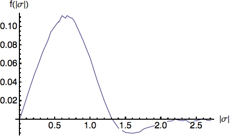
Figure 1: Intermediate numerical result for the evaluation of $I_{{\cal B},\theta}$.

To perform the six-dimensional numerical integration we have used the NIntegrate function of Mathematica™with the adaptive Monte Carlo method. To obtain Fig. 1 we increased $|\sigma|$ in steps of 0.05 from 0 to 2.7, with smaller step sizes around the maximum of $f(|\sigma|)$. For values of $|\sigma|$ that are larger than 3 it becomes impossible to obtain accurate results, but within the limitations of the numerical methods the results are consistent with a decreasing function $f(|\sigma|)$.

The last step in the numerical evaluation is to numerically integrate the function $f(|\sigma|)$. This can be done with standard methods and yields $I_{{\cal B},\theta}\approx 0.078$. The full result for the HV upper bound is then given by

$$\langle\hat{{\cal B}}^{2}\rangle_{\text{HV}} =I_{1,1}-2I_{\theta,1}-2I_{{\cal B},\theta}\;\;\approx 1.27.$$ (103)

References

- Bell (1964) J. S. Bell, Physics 1, 195 (1964).
- Clauser et al. (1969) J. F. Clauser, M. A. Horne, A. Shimony, and R. A. Holt, Phys. Rev. Lett. 23, 880 (1969).
- Freedman and Clauser (1972) S. J. Freedman and J. F. Clauser, Phys. Rev. Lett. 28, 938 (1972).
- Aspect et al. (1982) A. Aspect, J. Dalibard, and G. Roger, Phys. Rev. Lett. 49, 1804 (1982).
- Weihs et al. (1998) G. Weihs, T. Jennewein, C. Simon, H. Weinfurter, and A. Zeilinger, Phys. Rev. Lett. 81, 5039 (1998).
- Giustina et al. (2013) M. Giustina, A. Mech, S. Ramelow, B. Wittmann, J. Kofler, J. Beyer, A. Lita, B. Calkins, T. Gerrits, S. W. Nam, R. Ursin, and A. Zeilinger, Nature 2013/04/14/online, 4 (2013).
- Einstein et al. (1935) A. Einstein, B. Podolsky, and N. Rosen, Phys. Rev. 47, 777 (1935).
- Reid et al. (2009) M. D. Reid, P. D. Drummond, W. P. Bowen, E. G. Cavalcanti, P. K. Lam, H. A. Bachor, U. L. Andersen, and G. Leuchs, Rev. Mod. Phys. 81, 1727 (2009).
- Leonhardt and Vaccaro (1995) U. Leonhardt and J. A. Vaccaro, J. Mod. Opt. 42, 939 (1995).
- Gour et al. (2004) G. Gour, F. C. Khanna, A. Mann, and M. Revzen, Phys. Lett. A 324, 415 (2004).
- Praxmeyer et al. (2005) L. Praxmeyer, B.-G. Englert, and K. Wódkiewicz, Europ. Phys. J. D 32, 227 (2005).
- Cavalcanti et al. (2007) E. G. Cavalcanti, C. J. Foster, M. D. Reid, and P. D. Drummond, Phys. Rev. Lett. 99, 210405 (2007).
- He et al. (2010) Q. Y. He, E. G. Cavalcanti, M. D. Reid, and P. D. Drummond, Phys. Rev. A 81, 062106 (2010).
- Malley (2004) J. D. Malley, Phys. Rev. A 69, 022118 (2004).
- Malley and Fine (2005) J. D. Malley and A. Fine, Phys. Lett. A 347, 51 (2005).
- Banaszek and Wódkiewicz (1999) K. Banaszek and K. Wódkiewicz, Phys. Rev. Lett. 82, 2009 (1999).
- Banaszek and Wódkiewicz (1998) K. Banaszek and K. Wódkiewicz, Phys. Rev. A 58, 4345 (1998).
- Revzen et al. (2005) M. Revzen, P. A. Mello, A. Mann, and L. M. Johansen, Phys. Rev. A 71, 022103 (2005).
- Ozorio de Almeida (2009) A. Ozorio de Almeida, in Entanglement and Decoherence. Foundations and modern trends, Vol. 768 (Springer, Berlin, 2009) pp. 157–219.
- Wigner (1932) E. Wigner, Phys. Rev. 40, 749 (1932).
- Folland (1989) G. B. Folland, Harmonic Analysis in Phase Space (Princeton University Press, Princeton, 1989).
- Royer (1977) A. Royer, Phys. Rev. A 15, 449 (1977).
- Grossmann (1976) A. Grossmann, Commun. Math. Phys. 48, 191 (1976).
- M. V. Karasev and T. A. Osborn (2004) M. V. Karasev and T. A. Osborn, J. Phys. A. 37, 2345 (2004).
- Revzen (2006) M. Revzen, Found. Phys. 36, 546 (2006).
- Kalev et al. (2009) A. Kalev, A. Mann, P. A. Mello, and M. Revzen, Phys. Rev. A 79, 014104 (2009).
- Kenfack and Życzkowski (2004) A. Kenfack and K. Życzkowski, J. Opt. B: Quantum Semicl. 6, 396 (2004).
- Benedict and Czirják (1999) M. G. Benedict and A. Czirják, Phys. Rev. A 60, 4034 (1999).
- Redhead (1987) M. Redhead, Incompleteness, Nonlocality and Realism (Clarendon, 1987).
- Malley (1998) J. D. Malley, Phys. Rev. A 58, 812 (1998).
- Fine (1982a) A. Fine, Phys. Rev. Lett. 48, 291 (1982a).
- Bobo (2010) I. G. Bobo, Quantum conditional probability: implications for conceptual change of science (Universidad Complutense de Madrid, 2010) iSBN: 978-84-693-3483-6.
- Beltrametti and Cassinelli (1981) E. Beltrametti and G. Cassinelli, The Logic of Quantum Mechanics (Addison -Wesley, 1981).
- Gleason (1957) A. M. Gleason, J. Math. Mech 6, 885 (1957).
- Busch and Lahti (1996) P. Busch and P. J. Lahti, J. Math. Phys. 37, 2585 (1996).
- Hemmick and Shakur (2012) D. L. Hemmick and A. M. Shakur, Bell’s Theorem and Quantum Realism (Springer, Heidelberg, 2012).
- Gudder (1979) S. Gudder, Stochastic methods in quantum mechanics (North Holland, New York, 1979).
- Fine (1982b) A. Fine, J. Math. Phys. 23, 1306 (1982b).
- Bell (1966) J. S. Bell, Reviews of Modern Physics 38, 447 (1966).
- Kochen and Specker (1968) S. Kochen and E. Specker, Indiana Univ. Math. J. 17, 59 (1968).
- Bracken et al. (1999) A. J. Bracken, H.-D. Doebner, and J. G. Wood, Phys. Rev. Lett. 83, 3758 (1999).
- Abramowitz and Stegun (1964) M. Abramowitz and I. A. Stegun, Handbook of mathematical functions (National Bureau of Standards, Washington, D.C., 1964).
- Cahill and Glauber (1969) K. E. Cahill and R. J. Glauber, Phys. Rev. 177, 1857 (1969).
- Gradshteyn and Ryzhik (2007) Gradshteyn and Ryzhik, Table of Integrals, Series, and Products, 7th Edition, edited by A. Jeffrey and D. Zwillinger (Academic Press, 2007).
- Braunstein and Caves (1990) S. L. Braunstein and C. M. Caves, Ann. Phys. 202, 22 (1990).