The Effect of Biased Communications
On Both Trusting and Suspicious Voters

Abstract

In recent studies of political decision-making, apparently anomalous behavior has been observed on the part of voters, in which negative information about a candidate strengthens, rather than weakens, a prior positive opinion about the candidate. This behavior appears to run counter to rational models of decision making, and it is sometimes interpreted as evidence of non-rational “motivated reasoning”. We consider scenarios in which this effect arises in a model of rational decision making which includes the possibility of deceptive information. In particular, we will consider a model in which there are two classes of voters, which we will call trusting voters and suspicious voters, and two types of information sources, which we will call unbiased sources and biased sources. In our model, new data about a candidate can be efficiently incorporated by a trusting voter, and anomalous updates are impossible; however, anomalous updates can be made by suspicious voters, if the information source mistakenly plans for an audience of trusting voters, and if the partisan goals of the information source are known by the suspicious voter to be “opposite” to his own. Our model is based on a formalism introduced by the artificial intelligence community called “multi-agent influence diagrams”, which generalize Bayesian networks to settings involving multiple agents with distinct goals.

1 Introduction

Historically, political decision-making has been modeled in a number of ways. Models that propose rational decision making on the part of voters must account for the fact that voters frequently have difficulty in responding to factual surveys on political issues. One resolution to this difficulty is to model candidate evaluation as an online learning process, in which a tally representing candidate affect is incremented in response to external information [13], after which the information itself is discarded. However, in a number of recent studies of political decision-making, apparently anomolous behavior has been observed on the part of voters, in which negative information about a candidate $k$ strengthens (rather than weakens) a prior positive opinion held about $k$ [5, 20] .

This behavior appears to run counter to rational models of decision making, and it is sometimes interpreted as evidence of non-rational “motivated reasoning” [11]. In motivated reasoning models, a voter will (1) evaluate the affect of new information—i.e., its positive or negative emotional charge, then (2) compare this to the affect predicted by current beliefs, and finally (3) react, where congruent information (i.e., information consistent with predicted affect) is processed quickly and easily, and incongruent information is processed by a slower “stop-and-think” process. “Stop-and-think” processing may include steps such as counter-arguing, discounting the validity of the information, or bolstering existing affect by recalling previously-assimilated information [14, 20].

Some evidence for the motivated reasoning hypothesis comes from hman-subject experiments using a dynamic process tracing environment (DPTE), in which data relevant to a mock election is presented as a dynamic stream of possibly relevant news items. In DPTE experiments, detailed hypotheses about political reasoning can be tested, for instance by varying the frequency and amount of incongruent information presented to voters in the mock election. Experimental evidence shows, for instance, that both political sophisticates and novices spend more time processing negative information about a liked candidate, and novices also spend longer processing positive information about a disliked candidate [20]. Most intriguingly, small to moderate amounts of incongruent information—e.g., negative information about a liked candidate—actually reinforce the prior positive view of the candidate [21].

This apparently anomalous effect—whereby information has the inverse of the expected impact on a voter—appears to be inconsistent with rational decision-making. In this paper, we show analytically that this “anomalous” effect can occur in a model of rational decision making which includes the possibility of deceptive information. The model makes another interesting prediction: it justifies as computationally effective and efficient a heuristic of pretending to believe information from a possibly-deceptive source if that source’s political preferences are the same as the voters.

In particular, we will consider a model in which there are two classes of voters, which we will call trusting voters and suspicious voters, and two types of information sources, which we will call unbiased sources and biased sources. Information from an unbiased source is modeled simply as data $D_{k}$ that probabilistically inform a voter about a candidate $k$’s positions. Trusting voters are voters that treat information about a candidate as coming from an unbiased source. We show that, in our model, new data about a candidate can be efficiently incorporated by a trusting voter, and anomalous updates (in which “negative” information increases support) are impossible.

Biased sources are information sources $j$ who plan their communications with a goal in mind (namely, encouraging trusting voters to vote in a particular way). To do this, $j$ will access some data $C_{k}$ which is communicated to them only (not to voters directly) and release some possibly-modified version $B_{k}$ of $C_{k}$, concealing the original $C_{k}$. $B_{k}$ is chosen based on the utility to $j$ of the probable effect of $B_{k}$ on a trusting voter $i$.

We then introduce suspicious voters. Unlike trusting voters, who behave as if communications were from unbiased sources, suspicious voters explicitly model the goal-directed behavior of biased sources.

The behavior of rational suspicious voters depends on circumstances—depending on the assumptions made, different effects are possible. If the partisan goals of the biased source $j$ and a suspicious voter $i$ are aligned, then a suspicious voter can safely act as if the information is correct—i.e., perform the same updates as a naive voter. Intuitively, this is because $j$ is choosing information $B_{k}$ strategically to influence a naive voter to achieve $j$’s partisan goals, and since $i$’s goals are the same, it is strategically useful for $i$ to “play along” with the deception; this intutition can be supported rigorously in our model. If the partisan goals of $j$ are unknown, then a rational suspicious voter $i$ may discount or ignore the information $B_{k}$; again, this intuition can be made rigorous, if appropriate assumptions are made. Finally, if the partisan goals of $j$ are known to be “opposite” those of $i$, then a rational suspicious voter may display the “anomalous” behavior discussed above: information $B_{k}$ that would cause decreased support for a suspicious voter will cause increased support for $i$. Intuitively, this occurs because $i$ recognizes that $j$ may be attempting to decrease support for candidate $k$, and since $i$ and $j$ have “opposite” partisan alignments, it is rational for $i$ to instead increase support.

In short, in this model, a negative communication about $k$ can have the effect opposite to one’s initial expectation; however, the apparent paradox is not due to motivated reasoning, but simply to imprecise planning on the part of $j$. In particular, $j$’s communication was planned by a biased source with the aim of influencing trusting voters, while in fact, $i$ is a suspicious voter.

Below, we will first summarize related work, and then flesh out these ideas more formally. Our model will be based on a formalism introduced by the artificial intelligence community called “multi-agent influence diagrams”, which generalize Bayesian networks to settings involving multiple agents with distinct goals.

2 Related work

This work is inspired for recent work on motivated reasoning and hot cognition in political contexts (for recent overviews, see [9, 19]). There is strong experimental evidence that information processing of political information involves emotion, and there recent research has sought to either collect empirical evidence for [20, 5], and and build models that explicate [12], the mechanisms behind this phenomenon.

The models of this paper are not intended to dispute role of emotion in political decision making. Indeed, our models reflect situations in which one party deliberately withholds or distorts information to manipulate a second party, and introspection clearly suggests that such situations will typically invoke an emotional response. However, work in social learning (e.g., [22]) and information cascades (e.g., [23]) shows that behaviors (such as “following the herd”) which appear to be driven by non-rational emotions may in fact be strategies that are lead to results that are evolutionarily desirable (if not always “rational” from the individual’s perspective.) Hence, the identification of emotional aspects to decision-making does not preclude rational-agent explanations; rather, it raises the question of why these mechanisms exist, what evolutionary pressures might cause them to arise, and whether or not those pressures are still relevant in modern settings. This paper makes a step toward these long-term goals by identifying cases in which behavior explainable by motivated reasoning models is also rational, for instance in the result of Theorem 2.

The explanation suggested here for anomalous, motivated-reasoning-like updating is based on a voter recognizing that a source may be biased, and correcting for that bias. While this explanation of anomalous updates is (to our knowledge) novel, it is certainly recognized that trust in the source of information is essential in political persuasion, and that a voter’s social connextions strongly influences political decision-making (e.g., [1]). More generally, empirical studies of persuasion substantiate a role of confirmatory bias and prior beliefs [7], and show that in non-political contexts (e.g., in investing), sophisticated consumers of information adjust for credibility, while inexperienced agents under-adjust.

The results of this paper are also related to models of media choice—for instance, research in which the implications of a presumed tendency of voters to seek confirmatory news is explored mathematically [4, 2, 8, 25]. Other analyses show why preferences for unbiased news lead to economic incentives to distort the news [3]. This paper does not address these issues, but does contribute by providing a rational-agent model for why such a confirmatory bias exists: in particular, Proposition 3 describes a strategy from using information from biased information sources with similar preferences as a voter. We notice that this strategy is both simple and computationally inexpensive, and might be preferable on these grounds to more complex strategies to “de-noise” biased information from sources with unknown preferences.

A further connection is to formal work on “talk games”, such as Crawford and Sobel’s model of strategic communication [6]. In this model, a well-informed but possibly deceptive “sender” sends a message to a “receiver” who (like our voter) takes an action that affects both herself and the sender. Variants of this model have explored cases in which information can only be withheld or disclosed, and disclosed information may be verified by the receiver [15]; cases where the receiver uses approximate “coarse” reasoning [16]; and cases where there is a mixed population of strategic and naive recievers, all of whom obtain information from senders acting strategically [17].

The analysis goals in “talk games” is different from the goals of this paper. whereas we investigate whether specific counter-intuitive observed behavior can arise in a plausible (not necessarily temporally stable) situation, this prior work primarily nalyzes the communication efficiency of a a system in equilibrium, Some of the results obtained for talk games are reminiscent of results shown here: for instance, Crawford and Sobel show that in equilibrium, signaling is more informative when the sender and reciever’s preferences are more similar. However, other results are less intuitive: for instance, in some models there is no deception at equilibrium [17]. We note that while equilibria are convenient to analyze, there is no particular reason to believe that natural political discourse reaches an equilibria.

Game theory has a long history in analyses of politics; in particular, writing in 1973, Shubik discusses possible applications of game theory to analysis of misinformation [24]. The tools used used in this paper arose from more recent work in artificial intelligence [10, 18], specifically analysis of multi-agent problem solving tasks, in which one agent explicitly models the goals and knowledge of another in settings involving probabilistic knowledge. One small contribution of this paper is introduction of a new set of mathematical techniques, which (to our knowledge) have not been previously used for analysis of political decision-making. We note however that while these tools are convenient, they are not absolutely necessary to obtain our results.

3 Modeling trusting voters

3.1 A model

Draft—to check: subscripts for $C,B,R$

$i$	a voter
$j$	a pundit
$k$	a candidate
$T_{i},T_{j}$	“target positions” for voter $i$ and source $j$
$T_{k}$	the position of a candidate $k$
$dom(T)$	the set of values taken on by random variable $T$
$S_{ik},S_{jk}$	similarity of a target position and a candidate
$D_{k}$	data about candidate $k$
$Y_{ik}$	the vote of $i$ for $k$
$U_{i}$	utility function for $i$
$C_{jk}$	data about $k$ that is known only to $j$
$B_{jk}$	biased variant of data $C_{jk}$ about $k$ that has been modified by $j$
$R_{jk}$	reputational cost to pundit $j$ of modifying $C_{jk}$ to $B_{jk}$
$P{{}^{\rm TrV}}(X|Y)$	a conditional probability computed using the trusting voter model
$P{{}^{\rm BiP}}(X|Y)$	a conditional probability computed using the biased pundit model
$P{{}^{\rm SuV}}(X|Y)$	a conditional probability computed using the suspicious voter model

Table 1: Notation used in the Paper

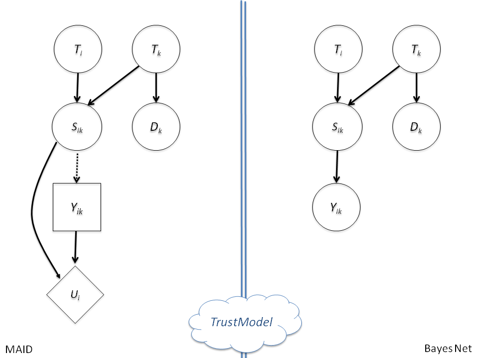
Figure 1: Model of a trusting voter, in MAID and Bayes Net notation

Consider the influence diagram on the left-hand side of Figure 1. In this model $i$ is a voter, and $k$ is a candidate. A voter $i$ has a preference $T_{i}$: for example, $T_{i}$ might be a member of the set

$$dom(T)=\{{\rm goodLiberal},{\rm evilLiberal},{\rm goodConservative},{\rm evilConservative}\}$$

Likewise $T_{k}$ is candidate $k$’s actual position, which is also an element of $dom(T)$. $S_{ik}$ measures how similar two positions are. $Y_{ik}$ is a measure of $i$’s support for $k$, which is chosen by voter $i$ to maximize $i$’s utility. The utility $U_{i}$ for voter $i$ is a function of how appropriate $Y_{ik}$ is given $S_{ik}$. Finally, $D_{k}$ is some data about $k$, generated probabilistically according to the value of $T_{k}$. As an example, this might be a statement made by $k$. The notation used in this diagram (and elsewhere below) is summarized in Table 1.

The shapes in the nodes in the diagrams indicate the type of the variable: diamonds for utilities, circles for random variables, and squares for decision variable, which an agent (in this case, voter $i$) will choose in order to maximize utility. The dotted arrow lines leading into a decision variable indicates information available when the decision is made. The arrows leading into a random variable node indicate “parents”—variables on which the value of the variable is conditioned. This sort of diagram is called an influence diagram, and the general version we will use later (in which multiple agents may exist) is called a MAID (Multi-Agent Influence Diagram) [18, 10].

More precisely the model defines a probability distribution generated by this process:

• Pick $t_{i}\sim P(T_{i})$, where $P(T_{i})$ is a prior on voter preferences.

• Pick $t_{k}\sim P(T_{k})$, where $P(T_{k})$ is a prior on candidate positions.

• Pick $d_{k}\sim P(D_{k}|T_{k}=t_{k})$. Equivalently, we could let $d_{k}=f_{D}(t_{k},\epsilon_{D})$, where $f_{D}$ is a function and $\epsilon_{D}$ is a random variable chosen independently of all other random variables in the model.

• Pick $s_{ik}\sim P(S_{kij}|T_{k}=t_{k},T_{j}=t_{j})$. Equivalently, we could let $s_{ik}=f_{S}(t_{i},t_{k},\epsilon_{S})$, where $f_{S}$ is a function and $\epsilon_{S}$ is a random variable, again chosen independently of all other random variables in the model.

• Allow voter $i$ to pick $y_{ik}$, based on a user-chosen probability distribution $P_{\tau}(Y_{ik}|S_{ik}=s_{ik})$, or equivalently computed using $f_{Y}(s_{ik},\epsilon_{Y})$.

• Pick utility $u_{i}$ from $P(U|y_{ik},s_{ik})$—or equivalently, computed as $u_{i}=f_{U}(y_{ik},s_{ik},\epsilon_{U})$.

The user can choose any distribution $P_{\tau}(Y|S)$, but we will henceforth assume that she will make the optimal choice—i.e., the probability distribution $P_{\tau}$ will be chosen by $i$ to maximize the expected utility $u_{i}$, where $u_{i}$ will be picked from $P(U|y_{ik},S_{ik})Pr(S_{ik})$—or equivalently computed as $u_{i}=\sum_{s^{\prime}}P(S_{ik}=s^{\prime})*f_{U}(y_{ik},s^{\prime},\epsilon_{U})$. In this specific case, the conversion is based on the observation that

$$P{{}^{\rm TrV}}(Y_{ik}=y|S_{ik}=s)=P\left(y={\rm argmax}_{y^{\prime}}\int_{\epsilon_{U}}f_{u}(y^{\prime},s,\epsilon_{U})d\epsilon_{U}\right)$$ (1)

and yields the Bayes network on the righthand side of Figure 1. Here $Y_{ik}$ is simply a random variable conditioned on $S_{ik}$, where the form of the dependency depends on Equation 1. Notice that the link from $S_{ik}$ to $Y_{ik}$ is deterministic. We call this the trusting voter model, since voter $i$ trusts the validity of the information $D_{k}$.

MAIDs (and their single-agent variants, influence diagram networks) have a number of advantages as a formalism. They provide a compact and natural computational representation for situations which are otherwise complex to describe - in particular, situations in which agents have limited knowledge of the game structure, or mutually inconsistent beliefs, but act rationally in accordance with these beliefs. In particular, MAIDs relax the assumption usually made in Bayesian games that players’ beliefs are consistent, and supports an explicit process in which one player can model another player’s strategy. MAIDs also support an expressive structured representation for a player’s beliefs. Together these features make them appropriate for modeling “bounded rationality” situations of the sort we consider here. Further discussion of MAIDs, and their formal relation to other formalisms for games and probability distributiobns, can be found elsewhere [10, 18].

Next, we will explore some simplifications of Eq. 1) If $f_{u}$ is deterministic, then Eq. 1 simplifies to the following choice of $y_{ik}$ given $s_{ik}$:

$$y_{ik}=f_{y}{{}^{\rm TrV}}(s_{ik})={\rm argmax}_{y^{\prime}}f_{u}(y^{\prime},s_{ik})$$

If only a distribution $P(S_{ik}=s)$ is known, then voter $i$’s optimal strategy is to let

$$y_{ik}={\rm argmax}_{y^{\prime}}\sum_{s}f_{u}(y^{\prime},s)P(S_{ik}=s)$$

In any case, however, the model has similar properties: once we assume that $i$ uses an optimal strategy, then the MAID becomes an ordinary Bayes net, defining a joint distribution over the variables $T_{i}$, $T_{k}$, $S_{ik}$, and $Y_{ik}$. We will henceforth use $P{{}^{\rm TrV}}$ to denote probabilities computed in this model, and reserve the non-superscripted $P(A|B)$ and $P(A)$ for conditional (respectively prior) probability distribution that are assumed to be available as background information.

$d$	$P(T_{i}=d)$
goodLiberal	0.4
goodConserv	0.4
evilLiberal	0.1
evilConserv	0.1
$d$	$P(T_{k}=d)$
goodLiberal	0.29
goodConserv	0.69
evilLiberal	0.01
evilConserv	0.01

$t_{i}$	$t_{k}$	$s_{ik}|t_{i},t_{k}$
goodLiberal	goodLiberal	$5+\epsilon$
goodLiberal	goodConserv	$1+\epsilon$
goodLiberal	evilLiberal	$-2+\epsilon$
goodLiberal	evilConserv	$-5+\epsilon$
goodConserv	goodConserv	$5+\epsilon$
goodConserv	evilLiberal	$-5+\epsilon$
goodConserv	evilConserv	$-2+\epsilon$
evilLiberal	evilLiberal	$5+\epsilon$
evilLiberal	evilConserv	$-5+\epsilon$
evilConserv	evilConserv	$5+\epsilon$

$t_{k}$	$c_{k}$	$P(c_{k}|t_{k})$
goodLiberal	safety-net	0.4
goodLiberal	motherhood	0.6
goodConserv	guns	0.3
goodConserv	motherhood	0.7
evilLiberal	safety-net	0.9
evilLiberal	chthulu	0.1
evilConserv	guns	0.8
evilConserv	chthulu	0.2
$P(Y_{i}=1|S_{ik}=s)$: see Eq 1

Table 2: Conditional probability tables (CPT) for a sample example of the trusting voter model. In the table for $s_{ik}|t_{i},t_{k}$, $\epsilon$ is drawn unformly from the set $\{-1,0,+1\}$ and for pairs $t_{i},t_{k}$ not shown, $s_{ik}|t_{i},t_{k}=s_{ik}|t_{k},t_{i}$.

Example 1

To take a concrete example, igure 2 shows the conditional probability tables for a small example, where candidates and target positions have values like evilLiberal and goodConserv, and the value of a communication $C_{k}$ is a name of something that a candidates might support (e.g.,motherhood or guns).

3.2 Implications of the model

3.2.1 New information about a candidate is easy to process

It is obvious how to use the trusting voter model to compute $Y_{ik}$ if $T_{k}$ and $T_{i}$ are known. However, a more reasonable situation is that $D_{k}$ and $T_{i}$ are known to $i$, but the true position of the candidate can only be inferred, indirectly, from $D_{k}$. Fortunately, using standard Bayes network computations, we can also easily compute a distribution over $Y_{ik}$ given $D_{k}$.

First, note that we can marginalize over $T_{k}$ and compute

$$P(D_{k}=d)={\sum_{t^{\prime}}P(D_{k}=d|t^{\prime})P(T_{k}=t^{\prime})}$$

and that using Bayes’ rule

$$P(T_{k}=t|D_{k}=d)=\frac{P(D_{k}=d|T_{k}=t)P(T_{k}=t)}{P(D_{k}=d)}=\frac{P(D_{k}=d|T_{k}=t)}{P(D_{k}=d)}P(T_{k}=t)$$ (2)

This gives a simple rule for $i$ to use in choosing her vote $Y_{ik}$ given $D_{k}$:

$$P{{}^{\rm TrV}}(Y=y|T_{i}=t_{i},D_{k}=d_{k})$$ (3)

$$= \sum_{s}P{{}^{\rm TrV}}(Y=y|S_{ik}=s)\sum_{t}P(S_{ik}=s|T_{i}=t_{i},T_{k}=t)P(T_{k}=t|D_{k}=d_{k})$$

$$= P{{}^{\rm TrV}}(Y=y|S_{ik})P(S_{ik}|t_{i},T_{k})P(T_{k}|d_{k})$$

The last line uses a simplified notation from the Bayes net community, where sums used to marginalize are omitted, and the event $X=x$ is replaced with $x$ when the variable $X$ is clear from context.

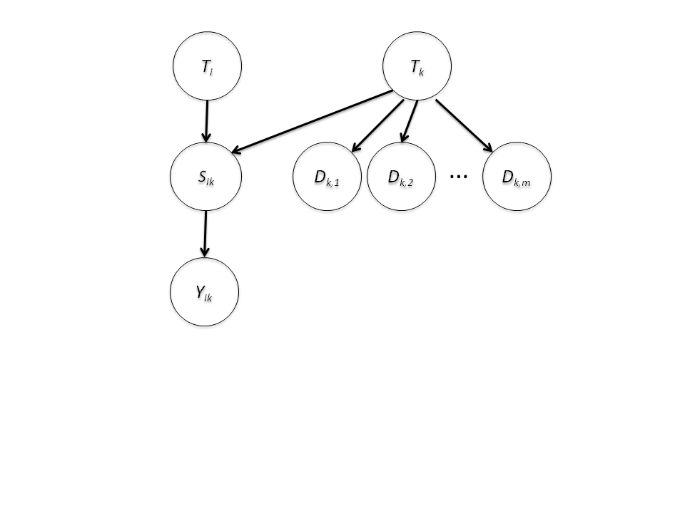
Figure 2: Model of a trusting voter with $m$ multiple independent data items about the candidate, in Bayes Net notation

This procedure can be extended easily to the case of multiple data items $D_{k,1},\ldots,D_{k,m}$ about the candidate, each independently generated from $P(D_{k}|T_{k})$, as shown in Figure 2. It can be shown that

$$P(T_{k}=t|d_{k,1},\ldots,d_{k,m})=\prod_{\ell}\frac{P(d_{k,\ell}|T_{k}=t)}{P(d_{k,\ell)}}P(T_{k}=t)$$

Put another way, we can define $P(T_{k}=t|d_{k,1},\ldots,d_{k,m})$ recursively as follows:

$$P(T_{k}=t|d_{k,1},\ldots,d_{k,m})=\frac{P(d_{k,m}|T_{k}=t)}{P{{}^{\rm TrV}}(d_{k,m)}}\cdot P(T_{k}=t|d_{k,1},\ldots,d_{k,m-1})$$

Hence, voter $i$ can quickly update beliefs about $T_{k}$ incrementally with each new piece of information $d_{k,\ell}$ and then (as before) use Equation LABEL:eq:y-from-tk to update her vote.

This incremental update property is worth emphasizing—while it may be complicated (if not computationally complex) to compute $P{{}^{\rm TrV}}(Y|S)$, or it may be difficult for a voter to establish her preferences $t_{i}$, absorbing new information in the trusting voter model is straightforward, and consists of two “natural” steps: estimating the candidate’s position $T_{k}$ given the information $d_{k,\ell}$; and then updating her support $y_{ik}$ for candidate $k$, given the updated estimate of the candidate’s position.

3.2.2 Positive information increases support

In a number of recent studies of political decision-making, negative information about a candidate $k$ has been observed to strengthen (rather than weaken) a voter’s support for $k$. We will show that under fairly reasonable assumptions this effect can not occur with the trusting voter model. In particular, we will assume that support $Y_{ik}$ increases monotonically with the similarity $S_{ik}$ of the candidate’s position $T_{k}$ and the voter’s preference $T_{i}$.

Recall that in the trusting voter model $Y_{ik}$ is a deterministic function of $S_{ik}$, defined as

$$f_{Y}{{}^{\rm TrV}}(s_{ik})={\rm argmax}_{y^{\prime}}\int_{\epsilon_{U}}f_{u}(y^{\prime},s,\epsilon_{U})d\epsilon_{U}$$ (5)

If $f_{Y}{{}^{\rm TrV}}$ has the property that

$$\forall s_{1}>s_{2},f_{Y}{{}^{\rm TrV}}(s_{1})\geq{}f_{y}{{}^{\rm TrV}}(s_{2})$$

then we will say that $i$’s support for $k$ increases monotonically with $s_{ik}$. This is one assumption needed for our result.

We also need to precisely define “negative” information. We say that $d_{k}$ is strictly negative about $k$ to voter $i$ if there is some partition of $dom(S_{ik})$ into triples $(a_{1},b_{1},\delta_{1})$, …,$(a_{m},b_{m},\delta_{m})$ so that

• For every triple $(a_{\ell},b_{\ell},\delta_{\ell})$, $a_{\ell}<b_{\ell}$, $\delta_{\ell}>0$, $P(S_{ik}=a_{\ell}|d_{k})=P(S_{ik}=a_{\ell})+\delta_{\ell}$, and $P(S_{ik}=b_{\ell}|d_{k})=P(S_{ik}=b_{\ell})-\delta_{\ell}$. In other words, learning $D_{k}=d_{k}$ shifts some positive probability mass $\delta_{\ell}$ from the larger similarity value $b_{\ell}$ to the smaller similarity value $a_{\ell}$.

• For all $s\in dom(S_{ik})$ that are not in any triple, $P(s_{ik}=s|d_{k})=P(s_{ik}=s)$. In other words, the probability mass of values $s$ not in any triples is unchanged.

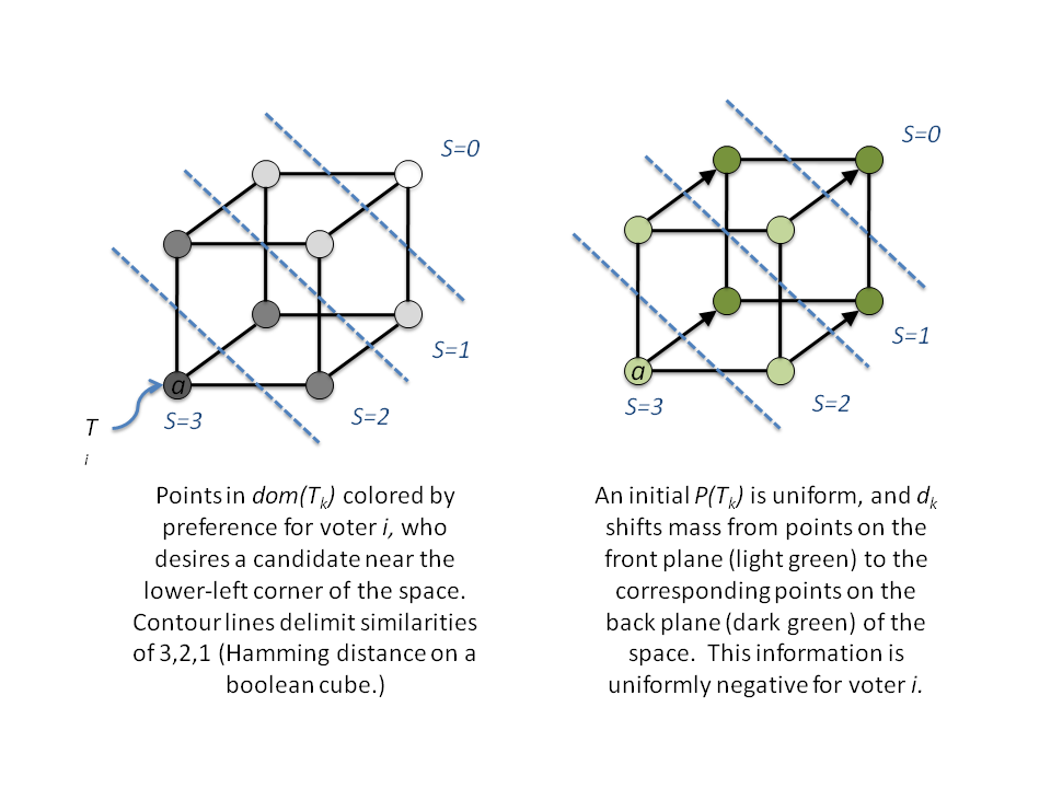
Figure 3: An illustration of strictly negative information for a voter $i$

To illustrate this, consider Figure 3, which illustrates a plausible example of strictly negative information. Strictly positive information is defined analogously.

We can now state formally the claim that negative information will reduce support. An analogous statement holds for strictly positive information.

Theorem 1

Let $E_{P}[X]$ denote the expected value of $X$ in probability distribution $P$. In a trusted voter model $P{{}^{\rm TrV}}$, if voter $i$’s support for $k$ increases monotonically with $s_{ik}$ and $d_{k}$ is strictly negative about $k$ to voter $i$, then $E_{P{{}^{\rm TrV}}}[Y_{ik}|D_{k}=d_{k}]<E_{P{{}^{\rm TrV}}}[Y_{ik}]$.

Proof. Let $S^{\prime}=dom(S_{ik})-\{a_{1},b_{1},\ldots,a_{m},b_{m}\}$, where the $a_{\ell},b_{\ell}$’s are the triples guaranteed by the strictly-negative property of $d_{k}$.

$$E_{P{{}^{\rm TrV}}}[Y_{ik}|D_{k}=d_{k}]$$

$$= \sum_{y}y\cdot P{{}^{\rm TrV}}(Y_{ik}=y|D_{k}=d_{k})$$

$$= \sum_{s}f_{y}{{}^{\rm TrV}}(s)P{{}^{\rm TrV}}(S_{ik}=s|D_{k}=d_{k})$$

$$= \sum_{s^{\prime}\in{}S^{\prime}}f_{y}{{}^{\rm TrV}}(s)P{{}^{\rm TrV}}(S_{ik}=s|d_{k})+\sum_{\ell=1}^{m}f_{y}{{}^{\rm TrV}}(a_{\ell})P{{}^{\rm TrV}}(S_{ik}=a_{\ell}|d_{k})+\sum_{\ell=1}^{m}f_{y}{{}^{\rm TrV}}(b_{\ell})P{{}^{\rm TrV}}(S_{ik}=b_{\ell}|d_{k})$$

Looking at the three terms of the final sum in turn, clearly

$$\sum_{s^{\prime}\in{}S^{\prime}}f_{y}{{}^{\rm TrV}}(s)P{{}^{\rm TrV}}(S_{ik}=s|d_{k})=\sum_{s^{\prime}\in{}S^{\prime}}f_{y}{{}^{\rm TrV}}(s)P{{}^{\rm TrV}}(S_{ik}=s)$$

and the last two terms can be written as

$$\sum_{\ell=1}^{m}f_{y}{{}^{\rm TrV}}(a_{\ell})P{{}^{\rm TrV}}(S_{ik}=a_{\ell}|d_{k})+f_{y}{{}^{\rm TrV}}(b_{\ell})P{{}^{\rm TrV}}(S_{ik}=b_{\ell}|d_{k})$$

$$= \sum_{\ell=1}^{m}f_{y}{{}^{\rm TrV}}(a_{\ell})\left(P{{}^{\rm TrV}}(S_{ik}=a_{\ell})+\delta_{\ell}\right)+f_{y}{{}^{\rm TrV}}(b_{\ell})\left(P{{}^{\rm TrV}}(S_{ik}=b_{\ell})-\delta_{\ell}\right)$$

$$= \sum_{\ell=1}^{m}f_{y}{{}^{\rm TrV}}(a_{\ell})P{{}^{\rm TrV}}(S_{ik}=a_{\ell})+f_{y}{{}^{\rm TrV}}(b_{\ell})P{{}^{\rm TrV}}(S_{ik}=b_{\ell})+\delta_{\ell}(f_{y}{{}^{\rm TrV}}(a_{\ell})-f_{y}{{}^{\rm TrV}}(b_{\ell}))$$

$$\leq \sum_{\ell=1}^{m}f_{y}{{}^{\rm TrV}}(a_{\ell})P{{}^{\rm TrV}}(S_{ik}=a_{\ell})+f_{y}{{}^{\rm TrV}}(b_{\ell})P{{}^{\rm TrV}}(S_{ik}=b_{\ell})$$

with the last step holding because (a) $\delta_{\ell}>0$ and (b) $a_{\ell}<b_{\ell}$. (Recall that from the monotonicity of $f_{y}$, if $a_{\ell}<b_{\ell}$ then $f_{y}{{}^{\rm TrV}}(a_{\ell})\leq{}f_{y}{{}^{\rm TrV}}(b_{\ell})$). Combining these gives that

$$E_{P{{}^{\rm TrV}}}[Y_{ik}|D_{k}=d_{k}]$$

$$= \sum_{s^{\prime}\in{}S^{\prime}}f_{y}{{}^{\rm TrV}}(s)P{{}^{\rm TrV}}(S_{ik}=s|d_{k})+\sum_{\ell=1}^{m}f_{y}{{}^{\rm TrV}}(a_{\ell})P{{}^{\rm TrV}}(S_{ik}=a_{\ell}|d_{k})+\sum_{\ell=1}^{m}f_{y}{{}^{\rm TrV}}(b_{\ell})P{{}^{\rm TrV}}(S_{ik}=b_{\ell}|d_{k})$$

$$\leq \sum_{s^{\prime}\in{}S^{\prime}}f_{y}{{}^{\rm TrV}}(s)P{{}^{\rm TrV}}(S_{ik}=s)+\sum_{\ell=1}^{m}f_{y}{{}^{\rm TrV}}(a_{\ell})P{{}^{\rm TrV}}(S_{ik}=a_{\ell})+f_{y}{{}^{\rm TrV}}(b_{\ell})P{{}^{\rm TrV}}(S_{ik}=b_{\ell})$$

$$= \sum_{s\in{}dom(S_{ik})}f_{y}{{}^{\rm TrV}}(s)P{{}^{\rm TrV}}(S_{ik}=s)=E_{P{{}^{\rm TrV}}}[Y_{ik}]$$

This concludes the proof.   $\blacksquare$

4 Modeling biased pundits and suspicious voters

4.1 Biased pundits

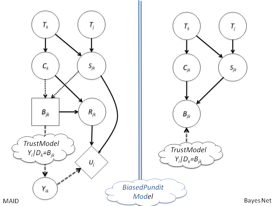
Figure 4: Model of a biased pundit, in MAID and Bayes net notation

We now consider a new model, as shown in Fig 4. In this model there is a pundit $j$, who, like a voter, has a target candidate position $T_{j}$. Pundit $j$ observes a private datapoint $C_{k}$ from candidate $k$—perhaps based on a private communication or research—and then publishes a “biased version” $B_{k}$ of $C_{k}$. However, $B_{k}$ is chosen under the assumption that some trusting voter $i$ will react to $B_{k}$ as if it were $D_{k}$ in the trusting voter model of Figure 1. Specifically, we assume that $B_{k}$ will provoke a vote $Y_{ik}$ according to the trusting voter model. The utility assigned by $j$ to this outcome is a function of $i$’s vote $Y_{ik}$, the similarity of $S_{jk}$ of $T_{k}$ to $j$’s target $T_{j}$, and a “reputational cost” $R_{jk}$, which is a function of $C_{k}$ and $B_{k}$. For instance, $R_{jk}$ might be zero if $b_{k}=c_{k}$, and otherwise some measure of how embarrassing it might be to $j$ if his deception of replacing $c_{k}$ with $b_{k}$ were discovered.

More precisely the model defines a probability distribution generated by this process:

• Pick $t_{j}\sim P(T_{j})$, where $P(T_{j})$ is a prior on pundit preferences.

• Pick $t_{k}\sim P(T_{k})$, where $P(T_{k})$ is a prior on candidate positions.

• Pick $c_{k}\sim P(D_{k}|T_{k}=t_{k})$, or equivalently, $c_{k}=f_{D}(t_{k},\epsilon_{D})$. (Notice that we assume $c_{k}$ is chosen from the same conditional distribution $P(D_{k}|T_{k})$ used in the trusting voter model to chose $D_{k}$—we’re using a different variable here to emphasize the different role it will play.)

• Allow pundit $j$ to pick $b_{k}$, based some user-chosen distribution $P_{\sigma}(B_{k}|C_{k}=c_{k})$.

• Pick $r_{ik}\sim P(R_{jk}|B_{k}=b_{k},C_{k}=c_{k})$, or equivalently, $r_{jk}=f_{R}(b_{k},c_{k},\epsilon_{R})$.

• Show $b_{k}$ to a trusting voter $i$, presenting it as a sample from $P(D_{k}|T_{k}=t_{k})$, and allow user $i$ to pick $y_{i}$ according to the trusting voter model.

• Pick $u_{i}\sim P(U_{j}|R_{jk}=r_{jk},S_{jk}=s_{jk},Y_{ik}=y_{ik})$, or equivalently, let $u_{j}=f_{U}(r_{jk},s_{jk},y_{jk},\epsilon_{U})$.

To distinguish the two utility functions, we will henceforth use $f_{U}{{}^{\rm TrV}}$ for the utility function $f_{U}(s,y)$ used in the trusting voter model, and use $f_{U}{{}^{\rm BiP}}$ for the utility function $f_{U}(r,s,y)$ defined above. As below, we will assume pundit $j$ will pick $b_{k}$, based on available estimates of $S_{ij}$ and knowledge of $C_{k}$, to maximize the expected utility $u_{j}$. This can be computed as

$$u_{j}=\sum_{r,s,y}P{{}^{\rm TrV}}(Y_{ik}=y|D_{k}=b_{k})P(S_{jk}=s|D_{k}=c_{k})P(R_{jk}=r|b_{k}=c_{k})f_{U}{{}^{\rm BiP}}(r,s,y,\epsilon_{U})$$

where $P{{}^{\rm TrV}}(Y_{ik}|D_{k}=b_{k})$ is estimated using the trusting voter model; $P(S_{jk}|D_{k}=c_{k})$ is computed as in Section 3.2.1, using $P(DC_{k}|T_{k})$ and $P(S_{jk}|T_{j},T_{k})$; and $P(R_{jk}=r|b_{k},c_{k})$ is computed using the given probability function of reputational cost $r$, as a function of the unbiased data $c_{k}$ and the biased version $b_{k}$ that is released.

Since pundit $j$ picks $B_{k}$ to maximize utility, then as before, we can convert this MAID to a Bayes net. Specifically, $B_{k}$ depends on the parents $C_{k}$ and $S_{jk}$ as follows.

$$P{{}^{\rm BiP}}(B_{k}=b|C_{k}=c,S_{jk}=s)=$$

$$P\left(b={\rm argmax}_{b^{\prime}}\sum_{r,y}P{{}^{\rm TrV}}(Y_{ik}=y|D_{k}=b_{k})P(R_{jk}=r|b^{\prime},c_{k})\int_{\epsilon_{U}}f_{U}{{}^{\rm BiP}}(r,s,y,\epsilon_{U})d\epsilon_{U}\right)$$

This can be simplified, if we assume that $f_{U}{{}^{\rm BiP}}$ and $f_{R}$ are deterministic:

$$P{{}^{\rm BiP}}(B_{k}=b|C_{k}=c,S_{jk}=s)=P\left(b={\rm argmax}_{b^{\prime}}\sum_{y}P{{}^{\rm TrV}}(Y_{ik}=y|D_{k}=b_{k})f_{U}{{}^{\rm BiP}}(f_{R}(b^{\prime},c),s,y)\right)$$ (6)

4.2 Suspicious voters

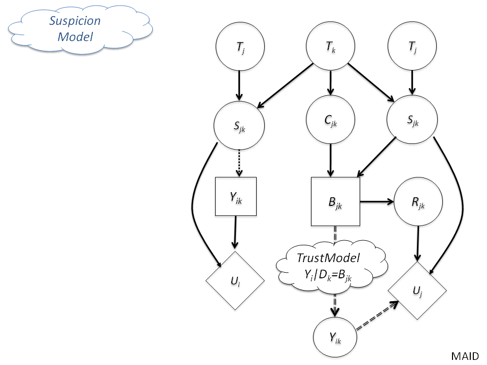
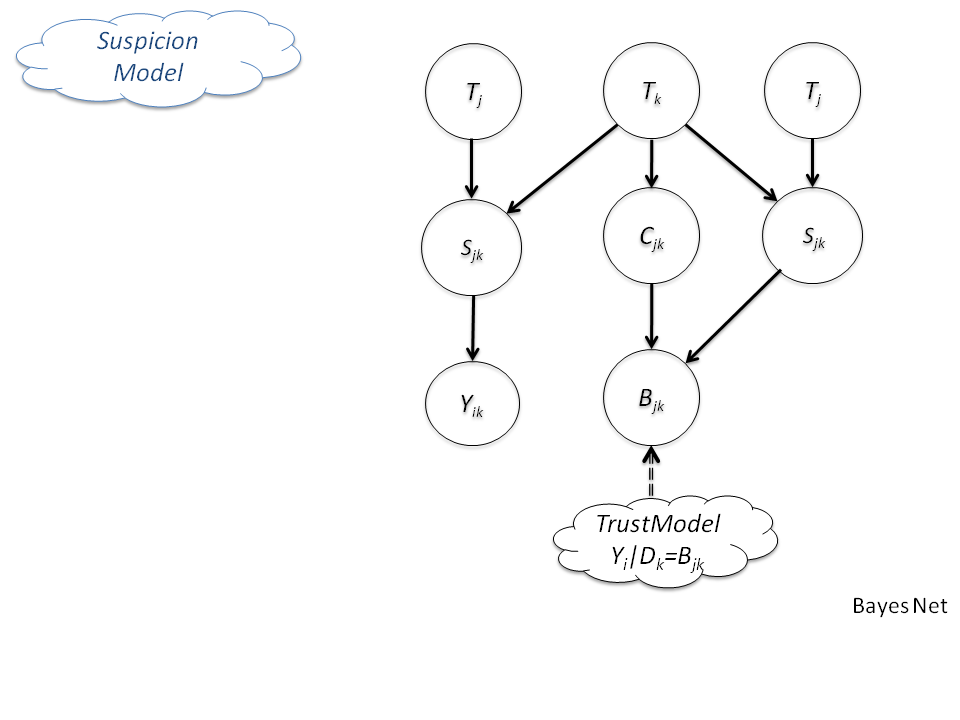
Figure 5: Model of a suspicious voter in MAID notation

Figure 6: Model of a suspicious voter in Bayes net notation

Finally, we introduce a model for a “suspicious voter”. Intuitively, this model is simple. As before, we assume that $j$ chooses $b_{k}$ according to the biased pundit model of Eq. 6—i.e., that $j$ believes $i$ to be a trusting voter. The suspicious voter will then attempt to reason with this correctly, and find the vote $Y_{i}$ maximizing $i$’s true utility, given then information revealed by $j$’s choice of $b_{k}$. The MAID and Bayes net versions of this model are shown in Figure 6 and Figure 6 respectively, and probabilities computed in this model will be writted as $P{{}^{\rm SuV}}$.

This suspicious voter model does not have a simple closed-form solution for $P{{}^{\rm SuV}}(S)$, as in the trusting voter model. The generative process for the suspicious voter model is identical to the biased pundit model, except that after $b_{k}$ is chosen according to Eq. 6, $i$ will pick a value of $Y_{ik}$ from a distribution $P{{}^{\rm SuV}}(Y_{ik}|B_{k}=b_{k})$, which is chosen to maximize the expected value of $u_{i}$. We will define

$$P{{}^{\rm SuV}}(Y_{ik}=y|S_{ik}=s)=P\left(y={\rm argmax}_{y^{\prime}}\int_{\epsilon_{U}}f_{u}(y^{\prime},s,\epsilon_{U})d\epsilon_{U}\right)$$

or, assuming determinacy,

$$y_{ik}=f_{y}{{}^{\rm SuV}}(s_{ik})={\rm argmax}_{y^{\prime}}f_{u}(y^{\prime},s_{ik})$$

This leads to a more complex inference problem for voters. Although the process of computing $P(S_{ik}|T_{i},T_{k})$ is unchanged, relative to the trusting voter model, a suspicious voter cannot estimate a distribution over $T_{k}$ using $d_{k}$, as in Eq. 2, because $d_{k}$ is not known. Instead $i$ only has indirect evidence about $d_{k}$ in the form of $b_{k}$.

However, voter $i$ can use this indirect evidence to compute

$$P{{}^{\rm SuV}}(T_{k}|B_{k}=b_{k})=\sum_{c}P{{}^{\rm TrV}}(T_{k}|D_{k}=c)\cdot P{{}^{\rm BiP}}(B_{k}=b|C_{k}=c)\cdot P{{}^{\rm TrV}}(D_{k}=c)$$ (7)

where $P{{}^{\rm BiP}}(b|c)=\sum_{t_{j}}P{{}^{\rm BiP}}(b|c,t_{j})P(t_{j})$ is the probability, in the biased pundit model, of pundit $j$ publishing $B_{k}=b$ when $C_{k}=c$. We can now break the summation over $c$ into two cases:

$$P{{}^{\rm SuV}}(T_{k}|B_{k}=b_{k})$$ (8)

$$= P{{}^{\rm TrV}}(T_{k}|D_{k}=b)\cdot P{{}^{\rm TrV}}(D_{k}=b)\cdot P{{}^{\rm BiP}}(B_{k}=b|C_{k}=b)$$

$$+ \sum_{c\not=b}P{{}^{\rm TrV}}(T_{k}|D_{k}=c)\cdot P{{}^{\rm TrV}}(D_{k}=c)\cdot P{{}^{\rm BiP}}(B_{k}=b|C_{k}=c)$$ (9)

In the term in line 8, $j$ is not altering the original input $c_{k}$, so we say he is being accurate. In line 9, so we say that $j$ is being deceptive. In order to exploit the information in $b_{k}$ using Eq  8-9 to optimize her utility, the suspicious voter must assess the probability of deception, and adjust inferences about candidate $k$ accordingly—a potentially difficult inference problem.

4.3 Implications of the suspicious voter model

To simplify further analysis, we will make some additional assumptions.

• We assume a deterministic reputational cost function $f_{R}$ in the biased pundit model.

• We assume the reputational cost of being accurate is zero, i.e., that $\forall c,f_{R}(c,c)=0$, and that the reputational cost of being deceptive is greater than zero, i.e., $\forall b\not=c,f_{R}(b,c)>0$.

• We assume deterministic utility functions $f_{U}{{}^{\rm TrV}}$ and $f_{U}{{}^{\rm BiP}}$.

• We assume the utility for pundits is the same as the utility for voters, minus the reputational cost of altering $c$ to $b$—i.e., that

  $$f_{U}{{}^{\rm BiP}}(r,s,y)\equiv f_{U}{{}^{\rm TrV}}(s,y)-r$$

Given these assumptions, some observations can now be made.

Proposition 1

If the prior $P(T_{j})$ such that $P{{}^{\rm BiP}}(b|c)=P{{}^{\rm BiP}}(b^{\prime}|c^{\prime})$ for all communications $b$, $b^{\prime}$, $c$ and $c^{\prime}$, then for all $b_{k}$, $P{{}^{\rm SuV}}(T_{k}|b_{k})=P{{}^{\rm SuV}}(T_{k})=P{{}^{\rm TrV}}(T_{k})$.

In other words, if $P{{}^{\rm BiP}}(b|c)$ is constant, then a biased pundit’s publications $b_{k}$ convey no information to $i$. This can be seen immediately by inspection of Eq. 7. Notice that requiring that $P{{}^{\rm BiP}}(b|c)$ does not imply that any individual pundits simply publish information $b$ uniformly at random, without regard to $c$—instead, it says that if one averages over all pundits and considers $\sum_{t_{j}}P{{}^{\rm BiP}}(b|c,t_{j})P(t_{j})$, then the cumulative probability of seeing any particular $b$ is constant, and independent of $c$.

More generally, one can make this observation.

Proposition 2

If the prior $P(T_{j})$ such that (1) $P{{}^{\rm BiP}}(c|c)=\alpha$ for all $c$, and (2) $P{{}^{\rm BiP}}(b|c)=P{{}^{\rm BiP}}(b^{\prime}|c)$ for all communications $b\not=c$ and $b^{\prime}\not=c^{\prime}$, then for all $b_{k}$,

$$P{{}^{\rm SuV}}(T_{k}|b_{k})=\alpha P{{}^{\rm TrV}}(T_{k}|b_{k})+(1-\alpha)P{{}^{\rm TrV}}(T_{k})$$

In other words, if all deceptions are equally likely, but publications are accurate with fixed probability $\alpha$, then a suspicious voter’s update to $T_{k}$ is simply a mixture of her prior belief $P{{}^{\rm SuV}}(T_{k})=P{{}^{\rm TrV}}(T_{k})$ and the belief a trusting voter would have, $P{{}^{\rm TrV}}(T_{k}|b_{k})$, with mixing coefficient $\alpha$. Again, this proposition can be be verified immediately by inspection of lines 8-9.

A final observation is that when a biased pundit’s preference $t_{j}$ is the same as a voter’s preference $t_{i}$, and this is known to both $i$ and $j$, then even a suspicious voter will obtain high utility by simply believing $j$’s publication $b_{k}$. In particular $i$’s utility from adopting the belief that $D=b_{k}$ is just as high as if $i$ had observed $c_{k}$ itself.

Proposition 3

If $t_{j}=t_{i}$, and $b_{k}$ is a publication from $j$ under the biased pundit model, then the expected utility to $i$ of voting according to $P{{}^{\rm TrV}}(T_{k}|D_{k}=b_{k})$ is at least as large as the expected utility to $i$ of voting according to $P{{}^{\rm TrV}}(T_{k}|D_{k}=c_{k})$.

This proposition seems plausible if we recall that $b_{k}$ was chosen to maximize the utility to $j$ of $i$’s belief in $b_{k}$ in the trusting voter model—thus, since the utility to $i$ is the same as the utility to $j$, it seems reasonable that adopting this belief is also useful to $i$. To establish it more formally, let us define $EU_{\ell}(b|c,t_{i})$ to be the expected utility to agent $\ell$ (either $i$ or $j$), absent reputational costs, of having $i$ adopt the belief in the trusting-voter model that $D_{k}=b$ when in fact $D_{k}=c$, if $T_{i}=t_{i}$. In other words, we define

$$EU_{\ell}(b|c,t_{i})\equiv\sum_{s_{\ell k},t_{k},y_{ik}}P{{}^{\rm TrV}}(T_{k}=t_{k}|D_{k}=c)P(S_{\ell k}=s_{\ell k}|t_{\ell},t_{k})P{{}^{\rm TrV}}(Y_{ik}=y_{ik}|T_{i}=t_{i},D_{k}=b)f{{}^{\rm TrV}}_{u}(s_{\ell k},y)$$

Note that the weighting in the factors $P{{}^{\rm TrV}}(T_{k}=t_{k}|D_{k}=c)P{{}^{\rm TrV}}(S_{\ell k}=s_{\ell k}|t_{\ell},t_{k})$ holds for both $i$ and $j$, because here we care about the true distribution over $T_{k}$, as deduced from $c$. The weighting in the factor $P{{}^{\rm TrV}}(Y_{ik}=y|T_{i}=t_{i},D_{k}=b)$ arises because for both $i$ and $j$, utility is based on $i$’s estimated support $y_{ik}$ for $k$ given $i$’s known preference $t_{i}$.

If we assume that $t_{i}=t_{j}=t$, then this simplifies to

$$EU_{i}(b|c,t_{i})=EU_{j}(b|c,t_{i})=\sum_{s,t_{k},y_{ik}}P{{}^{\rm TrV}}(T_{k}=t_{k}|D_{k}=c)P{{}^{\rm TrV}}(S=s|t,t_{k})P{{}^{\rm TrV}}(Y_{ik}=y_{ik}|T_{i}=t,D_{k}=b)f_{u}(s,y)$$

and hence we see that in this case, the functions for $i$ and $j$ are indeed the same. Since $j$ has chosen $b$ to maximize $EU_{\ell}(b|c)-f_{R}(b,c)$, and $f_{R}$ is never negative, clearly $EU_{j}(b|c,t_{i})\geq EU_{j}(b|c,t_{i})$, and so $EU_{i}(b|c,t_{i})\geq EU_{i}(b|c,t_{i})$ as well.

As noted in Section 2, there are a number of papers analyzing media bias in which voters are assumed prefer “good news” (i.e., new biased towards their favored candidates) leading to fragmentation and specialization as media companies differentiate by providing news biased for their readers. The results above suggest a rational reason for picking a news source $j$ with the same partisan preferences as one’s self: in particular, this sort of news is computionally easier to process. Similarly, biased sources with unknown preferences are “less informative”, in the sense that new information leads to changes in support (relative to unbiased sources, or well-aligned partisan sources).

4.4 Suspicious voters and “irrationality”

Finally, we address the question of whether suspicous voters can behave in the counter-intuitive manner discussed in the introduction—whether information about the candidate $k$ that is negative (as interpreted by a trusting voter) can increase support for a suspicous voter. We will show that this is possible.

Theorem 2

It can be the case that information $b$ will decrease $i$’s support for $k$ in the trusted voter model, and increase $i$’s support for $k$ in the suspicous voter model: i.e., it may be that $E_{P{{}^{\rm TrV}}}[Y_{ik}|D_{k}=b]<E_{P{{}^{\rm TrV}}}[Y_{ik}]$ but $E_{P{{}^{\rm SuV}}}[Y_{ik}|D_{k}=b]>E_{P{{}^{\rm SuV}}}[Y_{ik}]$.

Intuitively, this happens when $i$ believes strongly that $j$ is being deceptive, and $i$ has different candidate preferences from $j$. The theorem asserts the existence of such behavior, so we are at liberty to make additional assumptions in the proof (preferably, ones that could be imagined to hold in reality).

In the proof, we assume that $j$’s preferences $T_{j}$ are known to $i$. This is plausible since context may indicate, for instance, that $j$ is a strong conservative. This does not affect the basic model, since we allow the case of an arbitrary prior on $T_{j}$.

We also assume that all information about candidates is either strictly positive for $i$ and strictly negative for $j$, or else strictly negative for $i$ and strictly positive for $j$. To see how this is possible, first imagine a hypercube-like space of candidate positions, as in Figure 3, and assume that $T_{i}$ and $T_{j}$ are on opposite corners of the cube. The cube might indicate, for example, positions on the environment, abortion, and increased military spending, with $i$ preferring the liberal position on all three and $j$ preferring the conservative positions. Then assume that all information indicates the probability of the candidate’s position along these three axis; in this case the assumption is satisfied.

Given these two assumptions, the statement of the theorem holds. First, we need a slightly stronger version of Theorem 1. Informally, this states that if $i$ has partial knowledge of $b$, but does know that $b$ is strictly negative for $i$, then $i$’s support for $k$ will be weakened.

Corollary 1

Suppose $H$ is a probability distribution over items of information $b$, and also $b$ is strictly negative for $i$ for every $b$ with non-zero probability in $H$. Let $P{{}^{\rm TrV}}(Y_{ik}|H)$ denote

$$\sum_{b}P{{}^{\rm TrV}}(Y_{ik}|D_{k}=b)P_{H}(b).$$

Then $E_{P{{}^{\rm TrV}}}[Y_{ik}|H]<E_{P{{}^{\rm TrV}}}[Y_{ik}]$.

Proof. For any item $s\in dom(S_{ik})$, it is clear that

$$P(Y|E)=\sum_{b}P(Y|b)P_{H}(b)$$

and also, by marginalization over the (unrelated) variable $H$, we see that $P(Y)=\sum_{b}P(Y)P_{H}(b)$. Since for all $b$ with non-zero probability under $H$ we have that $E[Y|b]<E[Y]$, the result holds. This concludes the proof.   $\blacksquare$

We can now prove Theorem 2.

Proof. Suppose information $b$ that is strictly negative for $i$ is observed by $i$, and consider again the formula for $P{{}^{\rm SuV}}(T_{k}|B_{k}=b_{k})$ given on lines 8 and 9. This shows that the suspicous voter will reason by cases. In one case, $j$ is being accurate, and the change in probability for $T_{k}$ is in the same direction as in the trusted voter model, and as noted above, this will lead to a belief update that decreases support for $k$. However, this change is down-weighted by the factor $P{{}^{\rm BiP}}(B_{k}=b|C_{k}=b)P{{}^{\rm TrV}}(D_{k}=b)$, which can be interpreted as the probability that $b$ was really observed times the probability that $j$ chooses to report accurately. We will assume that $P{{}^{\rm TrV}}(D_{k}=b)$ is very small, so that

$$P{{}^{\rm SuV}}(T_{k}|B_{k}=b_{k})\approx\sum_{c\not=b}P{{}^{\rm TrV}}(T_{k}|D_{k}=c)\cdot P{{}^{\rm TrV}}(D_{k}=c)\cdot P{{}^{\rm BiP}}(B_{k}=b|C_{k}=c)$$

In this case, $j$ is being deceptive.

Reasoning is this case is complicated by the fact that $i$ must consider all inputs $c$ that could have observed, and compute the product of $P{{}^{\rm TrV}}(D_{k}=c)$, the prior probability of $c$, and also $P{{}^{\rm BiP}}(B_{k}=b|C_{k}=c)$, the probability of $b$ being reported in place of $c$ by $j$. However, since the preferences of $i$ and $j$ are opposite, the latter is quite informative: in particular, since $b$ was deceptively chosen by $j$ to be negative for $i$, then $b$ must prefer that $i$ give weaker support for $k$, implying that $c$ is actually negative for $j$, and hence positive for $i$. This holds for every $c$ that could have let to the deceptive report $b$. By Corollary 1, the net change in support for $i$ in the suspicous voter model positive. This concludes the proof.   $\blacksquare$

5 Concluding Remarks

To summarize, we propose a model in which there are two classes of voters, trusting voters and suspicious voters, and two types of information sources, unbiased sources and biased sources. Information from an unbiased source is modeled simply as observations $D_{k}$ that probabilistically inform a voter about a candidate $k$’s positions, and trusting voters are voters that treat information about a candidate as coming from an unbiased source. We show that reasoning about new information is computationally easy for trusting voters, and that trusting voters behave intuitively: in particular, negative information about candidate $k$ (according to a particular definition) will decrease support for $k$, and positive information will increase support.

Biased sources are information sources $j$ who plan their communications in order to encourage trusting voters to vote in a particular way). To do this, they report some possibly-modified version $B_{k}$ of a private observation $C_{k}$, concealing the original $C_{k}$. In the model, $B_{k}$ is chosen based on the utility to $j$ of the probable effect of $B_{j}$ on a trusting voter $i$.

Finally, suspicious voters model the behavior of biased sources. In general this is complicated to do, however, some special cases lead to simple inference algorithms. For instance, under one set of assumptions, all information from biased sources can be ignored. In another set of assumptions, a suspicious voter will make the same sort of updates to her beliefs as a trusting voter, but simply make them less aggressively, discounting the information by a factor related to the probability of deception.

Another interesting tractible reasoning case for suspicious voters is when the biased information source $j$ has the same latent candidate preferences as the voter $i$. In this case, suspicious voters can act the same way a trusting voter would—even if the information acted on is false, it is intended to achieve a result that is desirable to $i$ (as well as $j$).

These results are of some interest in light of the frequently-observed preference for partisan voters to collect information from similarly partisan information channels. The results suggest a possibly explanation for this, in terms of information content. The optimal way to process information from a possibly-deceptive unknown source, or a source with a known-to-be-different partisan alignment, is to either discount it, ignore it, or else employ complicated (and likely computationally complex) reasoning schemes. However, reports from partisan source with the same preferences as a voter can be acted on as if they were trusted—even if the reports are actually deceptive.

Finally, we show rigorously that a suspicious voter can, in some circumstances, increase support for a candidate $k$ after receiving negative information about $k$. Specifically, information that would decrease support for a trusting voter might increase support for a suspicious voter—if she believes the source has different candidate preferences, and if she believes the source is being deceptive. This behavior mimics behavior attributed elsewhere to “motivated reasoning”, but does not arise from “irrationality”—instead it is a result of the voters correct identification of, and compensation for, an ineffective attempt at manipulation on the half the information source.

We should note that this hypothesis does not suggest that emotion is not present in such situations—in fact, it seems likely that reports viewed as deceptive would indeed provoke strong emotional responses. It does suggest that some of the emotion associated with these counterintuitive updates may be associated with mechanisms that have an evolutionary social purpose, rather than being a result of some imperfect adaption of humans to modern life.

It seems plausible that additional effects can be predicted from the suspicious-voter model. For instance, although we have not made this conjecture rigorous, if a biased source $j$ does not know $i$’s political preferences, then deceptive messages $b$ will likely tend to be messages that would be interpreted as negative by most voters. For instance, $j$ might assert that the candidate violates some cultural norm, or holds an extremely unpopular political views. (Or , on the other hand, assert the candidate has a property that almost all voters agree is “good”. Arguably, most information from deceptive partisan sources would be of this sort, rather than discussion of stands on widely-disagreed-on issues (like gay marriage or abortion in the US).

As they stand, however, the results do suggest a number of specific predictions about how information might be processed in a social setting. First, information provided by persons believed to have political alignments similar to voter $i$ will be more easily assimilated, and have more effect on the view of $i$, than information provided by persons believed to have different political alignments. Second, information provided by persons with political alignments similar to voter $i$ will be more assimilated in roughly the same speed (and with the same impact) as information from a believed-to-be-neutral source. Third, information provided by persons with political alignments different from voter $i$ may lead to counterintuitive updates, while information from similarly-aligned sources or neutral sources will not. An important topic for future work would be testing these predictions, for instance using the DPTE methodology.

References

- [1] P.A. Beck, R.J. Dalton, S. Greene, and R. Huckfeldt. The social calculus of voting: Interpersonal, media, and organizational influences on presidential choices. American Political Science Review, 96(01):57–73, 2002.
- [2] D. Bernhardt, S. Krasa, and M. Polborn. Political polarization and the electoral effects of media bias. Journal of Public Economics, 92(5-6):1092–1104, 2008.
- [3] Jeremy Burke. Unfairly balanced: Unbiased news coverage and information loss. In Annual Meeting of the American Political Science Association, Chicago, IL, 2007.
- [4] M. Burke, E. Joyce, T. Kim, V. Anand, and R. Kraut. Introductions and requests: Rhetorical strategies that elicit online community response. In Proceedings of the The third communities and technologies conference, New York, NY, page 21–40, 2007.
- [5] Andrew J. W. Civettini and David P. Redlawsk. Voters, emotions, and memory. Political Psychology, 30(1):125–151, 2009.
- [6] V. P Crawford and J. Sobel. Strategic information transmission. Econometrica: Journal of the Econometric Society, page 1431–1451, 1982.
- [7] S. DellaVigna and M. Gentzkow. Persuasion: Empirical evidence. Annual Review of Economics, 2:643–670, 2010.
- [8] J. Duggan and C. Martinelli. A spatial theory of media slant and voter choice. The Review of Economic Studies, 78(2):640, 2011.
- [9] D.A. Graber and J.M. Smith. Political communication faces the 21st century. Journal of Communication, 55(3):479, 2005.
- [10] D. Koller and B. Milch. Multi-agent influence diagrams for representing and solving games. Games and Economic Behavior, 45(1):181–221, 2003.
- [11] Z Kunda. The case for motivated reasoning. Psychological Bulletin, 108(3):480–498, 1990.
- [12] M. Lodge, C. Taber, and C. Weber. First steps toward a Dual-Process accessibility model of political beliefs, attitudes, and behavior. Feeling politics: Emotion in political information processing, page 11–30, 2006.
- [13] Milton Lodge, Kathleen M. McGraw, and Patrick Stroh. An impression-driven model of candidate evaluation. The American Political Science Review, 83(2):pp. 399–419, 1989.
- [14] Milton Lodge and Charles Taber. Three Steps toward a Theory of Motivated Political Reasoning, pages 183–213. Cambridge University Press, 2000.
- [15] P. Milgrom and J. Roberts. Relying on the information of interested parties. The RAND Journal of Economics, page 18–32, 1986.
- [16] S. Mullainathan, J. Schwartzstein, and A. Shleifer. Coarse thinking and persuasion. The Quarterly Journal of Economics, 123(2):577, 2008.
- [17] M. Ottaviani and F. Squintani. Naive audience and communication bias. International Journal of Game Theory, 35(1):129–150, 2006.
- [18] A. Pfeffer. Networks of influence diagrams: A formalism for representing agents’ beliefs and decision-making processes. Journal of Artificial Intelligence Research, 33:109–147, 2008.
- [19] D. P Redlawsk. Feeling politics: Emotion in political information processing. Palgrave Macmillan, 2006.
- [20] David P. Redlawsk. Hot cognition or cool consideration? testing the effects of motivated reasoning on political decision making. The Journal of Politics, 64(04):1021–1044, 2002.
- [21] David P. Redlawsk, Andrew J. W. Civettini, and Karen M. Emmerson. The affective tipping point: Do motivated reasoners ever “get it”? Political Psychology, 31(4):563–593, 2010.
- [22] L. Rendell, R. Boyd, D. Cownden, M. Enquist, K. Eriksson, M. W. Feldman, L. Fogarty, S. Ghirlanda, T. Lillicrap, and K. N. Laland. Why copy others? insights from the social learning strategies tournament. Science, 328(5975):208, 2010.
- [23] M. J Salganik, P. S Dodds, and D. J Watts. Experimental study of inequality and unpredictability in an artificial cultural market. Science, 311(5762):854, 2006.
- [24] Martin Shubik. Game theory and political science. Paper No. 351, 1973.
- [25] D.F. Stone. Ideological media bias. Journal of Economic Behavior & Organization, 78:256–271, 2011.