The association problem in wireless networks: a Policy Gradient Reinforcement Learning approach

Abstract

The purpose of this paper is to develop a self-optimized association algorithm based on Policy Gradient Reinforcement Learning (PGRL), which is both scalable, stable and robust. The term robust means that performance degradation in the learning phase should be forbidden or limited to predefined thresholds. The algorithm is model-free (as opposed to Value Iteration) and robust (as opposed to Q-Learning). The association problem is modeled as a Markov Decision Process (MDP). The policy space is parameterized. The parameterized family of policies is then used as expert knowledge for the PGRL. The PGRL converges towards a local optimum and the average cost decreases monotonically during the learning process. The properties of the solution make it a good candidate for practical implementation. Furthermore, the robustness property allows to use the PGRL algorithm in an “always-on” learning mode.

Keywords: Wireless Networks, Queuing Theory, Stability, Load Balancing, Self Organizing Networks (SON), Reinforcement Learning, Policy Gradient, Self-Optimization.

I Introduction

The association problem in wireless networks has received considerable interest in the past few years due to its various applications. First, the mobile network landscape has become more and more heterogeneous. The network operator often needs to manage different radio access technologies such as Global System for Mobile Communications (GSM), High Speed Downlink Packet Access (HSDPA), Long Term Evolution (LTE), and Wireless Local Area Network (WLAN). In this context, connecting to a network with lower load by means of advanced Radio Resource Management (RRM) algorithms, via both mobility and selection/re-selection mechanisms, can significantly impact network performance and perceived QoS (see for example [1]). The complexity of managing resources in highly heterogeneous networks has been one of the drivers for the new paradigm of partial shift of the resource management burden from the network to the user terminals which can learn how to take intelligent association decisions ([2, 3]).

The renewed interest in the association problem has appeared with the introduction of Self-Organizing Networks (SON) in 4th Generation (4G) mobile networks. SON covers self-configuration, self-optimization and self-healing (automatic troubleshooting). In LTE, SON has already been introduced in the first Release (Release 8) of the standard [4]. The intra-system mobility load balancing optimization, which is closely related to the association problem, is one of the first self-optimization features introduced in the LTE standard [5].

Self-optimization aims at adapting the network to traffic variations and to new conditions of operation. The self-optimization process can be performed by autonomously adjusting network parameters such as parameters of RRM algorithms. The adoption of self-optimizing functionalities in real operating networks introduces strict requirements such as scalability and stability. Scalability means that the SON features should operate correctly when deployed in many network nodes, such as base stations and their neighboring ones. Stability means that the network empowered by the SON functionality diminishes congestion in the network so that the number of active users remains bounded and tends to a stationary regime. This stability definition corresponds to the stability in queuing systems.

Deriving optimal parameters or controllers via a learning process such as Reinforcement Learning (RL) ([6]) often requires a learning (or exploration) phase. Monotonic performance improvement during the learning phase is sought. We call this property robust learning.

The purpose of this paper is to develop a self-optimized association algorithm based on PGRL, which is both scalable, stable and robust. The requirement of robustness excludes direct application of RL solutions such as Q-Learning ([6]). Value Iteration ([6]) does not apply either since we assume no knowledge of the system dynamics, namely the transition probabilities of the Markov Decision Process (MDP). The association problem is modeled as a MDP, (cf. [7, 6]), and its optimal policy is derived for a small size problem to learn a functional form and to parameterize the policy space. Then, the obtained solution is used as expert knowledge for the PGRL ([8, 9, 10]). The PGRL converges to a local optimum and the average cost decreases monotonically during the learning phase. This makes it a good candidate for practical implementation. Furthermore, the robustness property allows to use the PGRL algorithm in a “always on” learning mode.
The contributions of the present paper are the following:

1. A queuing model for the problem of association in wireless networks is stated. This model takes into account flow-level dynamics allowing to optimize end-to-end, user-level performance indicators such as network capacity or mean file transfer time.

2. It is shown that the static association problem is tractable by classical convex optimization techniques.

3. The dynamic association problem is modeled as a MDP. A reinforcement learning (on-line learning) solution is proposed, and its convergence to a local optimum is proven. The approach is scalable when the number of Base Station (BS) increases, enabling to develop a practical solution.

4. A heuristic scheme is proposed which allows the algorithm to operate in a fully distributed manner and to greatly improve the accuracy of the gradient estimates.

The paper is organized as follows. Section II describes the system model for a wireless network serving elastic traffic, taking into account flow-level dynamics, and states the association problem. Section III examines the static version of the association problem, and shows that the problem is tractable by classical convex optimization techniques. Section IV presents the dynamic case, and models it as a MDP. A family of parameterized policies is introduced, allowing to develop a scalable reinforcement learning approach when the number of BSs grows. A heuristic which allows the algorithm to operate in a fully distributed manner and to improve the accuracy of the gradient estimation is introduced. Section V presents numerical experiments showing that the proposed method effectively increases the network capacity, and that the proposed heuristic considerably improves the accuracy and convergence speed of the method. Section VI concludes the paper.

II System model and problem statement

We describe here the system model encompassing the PHY, MAC and application layers. For each layer, we summarize relevant results in the literature and state the association problem. We consider the downlink of a wireless network, serving elastic traffic. The system bandwidth is $W$, under full reuse. The network area is $\mathbb{A}\subset\mathbb{R}^{2}$, and we assume it to be bounded. We denote by $N_{s}$ the number of BSs.

II-A Physical layer

Consider a single user located at $r\in\mathbb{A}$, served by BS $s$ with $1\leq s\leq N_{s}$ . We write $S_{s}(r)$ its Signal to Interference plus Noise Ratio (SINR). We consider Additive White Gaussian Noise (AWGN) and channel fading. We assume that the fading process is ergodic. We assume block fading i.e the fading process remains constant for the duration of a codeword. We treat the interference as Gaussian noise. We consider that full Channel State Information (CSI) is available at the receiver. Given $Z\in\mathbb{C}$ a value of the fading process, the data rate of a user is given by a certain function $\phi$:

$$\phi(|Z|^{2}S_{s}(r))\leq W\log_{2}(1+|Z|^{2}S_{s}(r))$$ (1)

For a large number of codewords, the time average of the the data rate of a user (1) is the ergodic data rate:

$$R_{s}(r)=E\left[\phi(|Z|^{2}S_{s}(r))\right]$$ (2)

II-B MAC layer

$n_{s}$ users are served simultaneously by BS $s$. For non-opportunistic scheduling, all users receive an equal part of the radio resources, and the throughput of a user located at $r$ is equal to $\frac{R_{s}(r)}{n_{s}}$. This corresponds to Round-Robin scheduling. In the case of opportunistic scheduling, each user is allocated the channel when its fading is the best. Define $\{Z_{i}\}_{1\leq i\leq n_{s}}$ independent and identically distributed (i.i.d) copies of $Z$, the throughput of a user located at $r$ is equal to:

$$E\left[(\prod_{i=2}^{n_{s}}{\bf 1}_{\{|Z_{i}|\leq|Z_{1}|\}})\phi(|Z_{1}|^{2}S_{s}(r))\right]$$ (3)

We approximate this quantity by $\frac{g(n_{s})R_{s}(r)}{n_{s}}$. The function $g$ is non-decreasing and denotes the multi-user diversity gain, and where $g(n_{s})\geq 1$. We write $g(\infty)=\underset{n_{s}\to+\infty}{\lim}\,g(n_{s})$ the maximal diversity gain. The non-opportunistic scheduling case can be seen as a particular case with $g\equiv 1$. Derivation of $g$ for particular channel models can be found in [11, 12, 13].

II-C Application layer

Consider users arriving randomly according to a spatial Poisson process on $\mathbb{A}\times\mathbb{R}^{+}$, with intensity $\lambda(dr\times dt)=\lambda drdt$. We write $\lambda_{tot}=\lambda\int_{\mathbb{A}}dr$ the total arrival rate. The arrival process is marked with $\sigma$, the file size to be downloaded and we assume independence between the arrival process and the file sizes. We write $\mathbb{A}_{s}\subset\mathbb{A}$ the area served by BS $s$. We say that the system is stable if the distribution of the number of active users tends to a stationary limit, and unstable if the number of active users grows to infinity. Such a system can be modeled by $N_{s}$ parallel M/G/1/PS (Processor Sharing) queues, and the following theorem summarizes the results on the system stability region and the mean performance (cf. [14]).

Theorem 1.

The load of BS $s$ is

$$\rho_{s}=\frac{\lambda E\left[\sigma\right]}{g(\infty)}\int_{\mathbb{A}_{s}}\frac{1}{R_{s}(r)}dr,$$ (4)

BS $s$ is stable if $\rho_{s}<1$ and unstable if $\rho_{s}>1$.
Consider non opportunistic scheduling and assume stability of BS $s$, and denote by $n_{s}(t)$ the mean number of active users served by BS $s$ in stationary regime at time $t$. Then we have that:

$$E\left[n_{s}(t)\right]=\frac{\rho_{s}}{1-\rho_{s}}$$ (5)

II-D The association problem

Now let us consider a new zone $\mathbb{A}_{0}\subset\mathbb{A}$. The association problem consists in allocating the traffic arriving in $\mathbb{A}_{0}$ to BSs, in order to optimize a given performance indicator. We distinguish two problems: the static association problem and the dynamic association problem.

In the static version, the traffic is attributed to BSs regardless of the current state of the system. Namely, $\mathbb{A}_{0}$ is partitioned into $N_{s}$, regions, and users arriving in the $s$-th region will be served by BS $s$ regardless of the number and locations of active users. In the dynamic problem, the system has access to the current user configuration to make a decision. Namely, the user configuration is composed of the number of active users, their locations, the BS they are currently attached to and their remaining amount of data to be downloaded. We call a policy a mapping between user configuration and association of each user. The problem consists in finding the policy that maximizes a given performance indicator.

II-E A finite set of data rates

In practical systems, there only exists a finite set of possible data rates, due to the finite number of modulation and coding schemes. This allows us to introduce a discretized version of the previous model, used in next sections. Let ${\cal I}\in\mathbb{N}$ denote the number of possible data rates, and $R^{(i)}$ - the $i$-th possible data rate. We use the convention $R^{(0)}=0$ and $R^{({\cal I}+1)}=+\infty$. We write

$$\mathbb{A}_{s,i}=\{r\in\mathbb{A}_{s}|R_{s}(r)\in[R^{(i)},R^{(i+1)})\}.$$ (6)

We assume that all users in $\mathbb{A}_{s,i}$ served by BS $s$ have a data rate of $R^{(i)}$.

We assume that $\mathbb{A}_{s,0}$ is empty, which can be enforced through admission control, namely, any user whose radio condition does not enable him to achieve even the lowest allowed data rate is not allowed to enter the system. $\mathbb{A}_{s}$ is partitioned into $\cup_{1\leq i\leq{\cal I}}\mathbb{A}_{s,i}$.

It is noted that the discretized model is a conservative model, since user data rates in the discretized model are lower bounds for the data rates in the continuous model. This is an important property since it implies that system performance given by the discrete model is a lower bound of the system performance in the continuous model, and instability in the continuous model implies instability in the discrete model as well.

We assume that $r\mapsto R_{s}(r)$ is measurable for all $s$, hence $\mathbb{A}_{s,i}$ are Borel sets for all $(s,i)$, and the integrals for the system performance in Theorem 1 are well-defined. We call users arriving in $\mathbb{A}_{s,i}$ users of class $(s,i)$. Their arrival rate is $\lambda_{s,i}=\lambda\int_{\mathbb{A}_{s,i}}dr$.

We partition $\mathbb{A}_{0}$ as well. We write $\mathbb{I}=\{0,\cdots,{\cal I}\}^{N_{s}}\setminus\{(0,\dots,0)\}$, we consider $I\in\mathbb{I}$ and denote by $I_{s}$ its $s$-th component. We define the zone associated to configuration $I$, $\mathbb{A}_{0,I}$, by:

$$\mathbb{A}_{0,I}=\{r\in\mathbb{A}_{0}|R_{s}(r)\in[R^{(I_{s})},R^{(I_{s}+1)}),1\leq s\leq N_{s}\}.$$ (7)

We have that $\mathbb{A}_{0}=\cup_{I\in\mathbb{I}}\mathbb{A}_{0,I}$. We denote users of class $(0,i)$ users that have arrived in $\mathbb{A}_{0,I}$. Their arrival rate is $\lambda_{0,I}=\lambda\int_{\mathbb{A}_{0,I}}dr$.

Figure 1 represents the model with $4$ possible data rates and $4$ BSs. The gray zones belong to $\mathbb{A}_{0}$ and can be served by any BS. The non-gray zones can only be served by the closest BS. Zone $\mathbb{A}_{1,4}$ is the closest to BS $1$ and can only be served by BS $1$ with data rate $R^{(4)}$. Zone $\mathbb{A}_{1,3}$ can only be served by BS $1$, but with lower data rate $R^{(3)}$ since it is further away from BS $1$. The gray zone $\mathbb{A}_{0,(2,1,1,1)}$ can be served by BS $1$ with data rate $R^{(2)}$ and by other BSs with data rate $R^{(1)}$, since it is closer to BS $1$. The central zone $\mathbb{A}_{0,(1,1,1,1)}$ can be served by all BSs with data rate $R^{(1)}$.

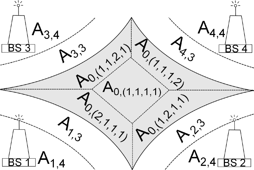
Figure 1: The association problem

The association problem is to determine the proportion of traffic from $\mathbb{A}_{0,I}$ to be served by BS $s$, for all $s$ and $I$.

II-F Numerical tractability

For each zone $\mathbb{A}_{0,I}$, $I\in\mathbb{I}$, we need to specify the amount of traffic which will be associated to each BS. There are $({\cal I}+1)^{N_{s}}-1$ such zones, and the number of variables needed for the association problem is $N_{s}(({\cal I}+1)^{N_{s}}-1)$. The number of variables grows exponentially with $N_{s}$ and makes the problem numerically intractable, simply from the memory required to store a solution. In practice, however, the vast majority of those zones will be empty. Namely, for a given zone $\mathbb{A}_{0,I}$, if there exists a BS $s$ such that the available data rate at station $s$ is high, then all the users arriving in $\mathbb{A}_{0,I}$ will be allocated to BS $s$ and generate little load. Hence $\mathbb{A}_{0}$ typically consists of cell edges zones. We will assume that there exists ${\cal I}_{edge}<{\cal I}$ such that, if users arriving in $\mathbb{A}_{0,I}$ can be served by a station $s$ at a rate larger than $R^{({\cal I}_{edge})}$ i.e $R^{(I_{s})}\geq R^{({\cal I}_{edge})}$, then they will all be served by BS $s$.

Furthermore, consider a location $r$, which is far away from the location of BS $s$. Then we will have $R_{s}(r)<R^{(1)}$ which means that no traffic from $\mathbb{A}_{0,I}$ shall be allocated to $s$ anyway. We say that $(s,r)$ is connected if $R_{s}(r)\geq R^{(1)}$ and we say that BSs $s$ and $s^{\prime}$ are neighbors if there exists a point $r$ such that $(s,r)$ and $(s^{\prime},r)$ are connected. We write $N_{neigh}$ the maximal number of neighbors for a BS. The actual number of variables can then be crudely upper bounded by $N_{s}N_{neigh}({\cal I}_{edge}^{N_{neigh}}-1)$ which only grows linearly $N_{s}$. Typical values are $N_{neigh}=6$ and ${\cal I}_{edge}=1$, for which we need $6N_{s}$ variables, and a large number of BSs can be easily handled.

III The static association problem

We consider non-opportunistic scheduling. We write $a_{s,I}\in[0,1]$ the proportion of users of class $(0,I)$ served by BS $s$. This can correspond to three different physical mechanisms, each of which might or might not be applicable depending on the network technology:

1. A user arriving in $\mathbb{A}_{0,I}$ attaches itself to BS $s$ with probability $a_{s,I}$.

2. A user arriving in $\mathbb{A}_{0,I}$ downloads a fraction $a_{s,I}$ of the requested file through BS $s$.

3. $\mathbb{A}_{0,I}$ is divided into $N_{s}$ sub-regions $\mathbb{A}_{0,I,s}$ the sizes of which are proportional to $a_{s,I}$. Namely:

   $$a_{s,I}=\frac{\int_{\mathbb{A}_{0,I,s}}dr}{\int_{\mathbb{A}_{0,I}}dr}$$ (8)

We define ${\bf a}=(a_{s,I})_{1\leq s\leq N_{s},I\in\mathbb{I}}$. Given ${\bf a}$, the load of BSs can be calculated as in Theorem 1:

$$\rho_{s}({\bf a})=E\left[\sigma\right]\left(\lambda\int_{\mathbb{A}_{s}}\frac{1}{R_{s}(r)}dr+\sum_{I\in\mathbb{I}}\frac{a_{s,I}\lambda_{s,I}}{R^{(I_{s})}}\right)$$ (9)

We write ${\bf\rho}({\bf a})=(\rho_{1}({\bf a}),\cdots,\rho_{N_{s}}({\bf a}))$.
Let us consider a convex function $U:\mathbb{R}^{N_{s}\times|\mathbb{I}|}\to\mathbb{R}$, the static association problem corresponds to the following optimization problem:

minimize $$U({\bf\rho}({\bf a}))$$ (10)

subject to $$a_{s,I}\geq 0 \;,\;1\leq s\leq N_{s} ,I\in\mathbb{I}$$ (11)

and $$\sum_{1\leq s\leq N_{s}}a_{s,I}=1 ,I\in\mathbb{I}$$ (12)

Such optimization problems bear strong resemblance with optimization problems encountered in routing.

Theorem 2.

Optimization problem (10) is convex.

Proof.

As seen in equation (9), ${\bf a}\mapsto{\bf\rho}({\bf a})$ is affine, hence by composition of an affine mapping with a convex function, we have that ${\bf a}\mapsto U({\bf\rho}({\bf a}))$ is convex. Similarly, constraints (11) and (12) are affine hence convex. ∎

Corollary 1.

The minimization of mean file transfer time is a particular case of (10), with

$$U({\bf\rho}({\bf a}))=\frac{1}{\lambda_{tot}}\sum_{1\leq s\leq N_{s}}\frac{\rho_{s}({\bf a})}{1-\rho_{s}({\bf a})}$$ (13)

Proof.

By Little’s law [15], the mean file transfer time is equal to the mean number of active users divided by the total arrival rate. From Theorem 1, the mean file transfer time is

$$\frac{1}{\lambda_{tot}}E\left[\sum_{1\leq s\leq N_{s}}n_{s}(t)\right]=\frac{1}{\lambda_{tot}}\sum_{1\leq s\leq N_{s}}\frac{\rho_{s}}{1-\rho_{s}}$$ (14)

Furthermore, let $x\in\mathbb{R}^{N_{s}}$, we have that

$$x\mapsto\frac{1}{\lambda_{tot}}.\frac{x_{s}}{1-x_{s}}=\frac{1}{\lambda_{tot}}\left(\frac{1}{1-x_{s}}-1\right)$$ (15)

which is convex and

$$x\mapsto\frac{1}{\lambda_{tot}}\sum_{1\leq s\leq N_{s}}\frac{x_{s}}{1-x_{s}}$$ (16)

is convex as a sum of convex functions. ∎

Theorem 2 shows that (10) is computationally tractable using classical convex optimization methods (see for example [16]), and it includes the important problem of minimizing the mean file transfer time. The reader can refer to the literature on routing in which such optimization problems have been studied extensively.

IV The dynamic association problem

IV-A MDPs and reinforcement learning

MDPs can be used to model optimal control problems where the system state has a markovian structure as described briefly below. The reader can refer to [7, 6] for a complete exposition of the topic.

We consider $(\Omega,\mathbb{P},{\cal F})$ a probability space. A MDP is defined by a discrete set of possible system states ${\cal S}$, a discrete set actions ${\cal A}$, an intensity matrix $\mu:{\cal S}^{2}\times{\cal A}\to\mathbb{R}^{+}$ , and a cost function $r:{\cal S}\times{\cal A}\times\Omega\to\mathbb{R}$.

Denote $R(s,a)=E\left[r(s,a,\omega)\right]$ the average cost. A policy is a mapping ${\cal S}\mapsto{\cal D}({\cal A})$, where ${\cal D}({\cal A})$ is the space of probability distributions on ${\cal A}$. Given a policy $P$ and $P(s,a)$ the probability of choosing action $a$ in state $s$ we write $\mu_{P}(s^{\prime},s)=\sum_{a\in{\cal A}}P(s,a)\mu(s^{\prime},s,a)$ the transition intensity from $s$ to $s^{\prime}$ under policy $P$.

Consider a policy $P$, we call the stochastic process $\{s_{t},a_{t},r_{t}\}$ a realization of the MDP for policy $P$ if:

• $a_{t}$ depends only on $s_{t}$ and is distributed according to $P(s_{t})$

• $\{s_{t}\}$ is a Markov process with intensity matrix $\mu_{P}(s^{\prime},s)$

• $r_{t}$ depends only on $(s_{t},a_{t})$, and is equal to $r(s_{t},a_{t})$ in distribution

The average cost of policy $P$ starting at $s\in{\cal S}$ can be defined by:

$$J_{P}(s)=\underset{T\to+\infty}{\limsup}\,\frac{1}{T}E\left[\int_{0}^{T}r_{t}dt\right].$$ (17)

Assume that $P$ is such that $\{s_{t}\}$ is ergodic, then $s\mapsto J_{P}(s)$ is constant and we write $J_{P}(s)=J_{P}$. In the following, we will use the hypothesis that the MDP is such that either $P$ makes $\{s_{t}\}$ ergodic, or else $J_{P}(s)=+\infty$. While this might first appear as a strong hypothesis, this is actually the case in a large number of problems such as queuing problems. Namely, either a policy makes the queue ergodic, or else the number of active users grows to infinity.

Solving the MDP consists then in finding the optimal policy which minimizes the cost $P^{*}=\underset{P}{\arg\min}\,J_{P}$. Existence and uniqueness results can be found in [7, 17].

The reinforcement learning problem is defined as deriving the optimal policy without the knowledge of the probabilistic structure of the model, through trial-and-error, cf. [6]. Namely, the intensity matrix $\mu$ and the distribution of the costs $r$ are unknown, and we can only obtain MDP realizations $\{s_{t},a_{t},r_{t}\}$. It is hence a simulation-based method or model-free method.

IV-B Resolution techniques and scalability

It is noted that by using discretization and “uniformization” (cf. [7]), we can always reduce the continuous time MDP to a discrete time MDP. In the remainder of the paper, whenever we employ reinforcement learning, it will be done using the discrete time version of the system.

When the intensity matrix and the distribution of the costs are known, and both ${\cal S}$ and ${\cal A}$ are is finite, the optimal policy can be derived via an iterative scheme, namely dynamic programming thanks to a fixed-point relation holding at optimality. In practice however, for large state spaces, this becomes numerically intractable (“curse of dimensionality”).

A scalable approach is to introduce a parameterized family of policies $\{P_{\theta},\theta\in\Theta\}$ and define the cost $J(\theta)=J_{P_{\theta}}$, once again using the previous hypothesis of ergodicity. This parameterization is a powerful idea for solving optimal control problems numerically with state spaces of large dimension. The problem becomes the optimization of $\theta\mapsto J(\theta)$, which is assumed to be computationally tractable. It is noted that the performance of such a scheme highly depends on the goodness of the chosen family of policies. Choosing a good parametrization generally implies having some knowledge on the structure of the optimal controller. It can be seen as a form of “expert knowledge”.

IV-C Policy gradient reinforcement learning approach

It remains to show how to optimize $\theta\mapsto J(\theta)$, without the knowledge of the probabilistic structure of the model. We assume that we are at least able to simulate the system for a fixed value of $\theta$, and that $J(\theta)$ can then be computed by averaging the observed cost for a sufficiently long simulation.
We are interested in both local and global optima. For global optima, since the problem is not convex in general, a search heuristic (e.g. genetic algorithm, particle swarm optimization) is needed, which requires to compute $J(\theta)$ for a large number of values of $\theta$.
For local optima, we can use a descent method by calculating $\nabla_{\theta}J(\theta)$. The crudest approach is to approximate the gradient using finite differences. We compute its $k$-th component by:

$$\frac{J(\theta+\epsilon e_{k})-J(\theta-\epsilon e_{k})}{2\epsilon},$$ (18)

for a small $\epsilon$, where $e_{k}$ stands for the $k$-th unit vector. This is possible whenever $J(\theta)$ can be computed, but requires a number of simulations equal to twice the number of components of $\theta$. Furthermore, this approach is not suitable for an “on-line” implementation where instead of simulating the system, the algorithm must compute an estimate of the gradient based on observations from a real network.
The approach we propose here consists in estimating $\nabla_{\theta}J(\theta)$ from a single (discrete-time) sample path $\{s_{t},a_{t},r_{t}\}_{t\in\mathbb{N}}$, using the method described in [9].

We write $\mathbb{P}_{\theta}$ the probability measure given policy $P_{\theta}$. It is possible to compute iteratively the eligibility traces:

$$z(t+1)=\beta z(t)+\frac{\nabla_{\theta}\mathbb{P}_{\theta}(a_{t}|s_{t})}{\mathbb{P}_{\theta}(a_{t}|s_{t})},$$ (19)

and the associated gradient estimates:

$$\Delta(t+1)=\Delta(t)+\frac{1}{t+1}(r_{t+1}z(t+1)-\Delta(t)).$$ (20)

The gradient estimates converge almost surely (a.s) to an ascent direction:

$$\liminf_{t\rightarrow+\infty}<\Delta(t),\nabla_{\theta}J(\theta)>\,\,>0.$$ (21)

IV-D Modeling the association problem as a MDP

We show that the association problem can be modeled as a continuous time MDP. We assume that association decisions are taken when users enter the system. This avoids the possibility of constant hand-overs every time the user configuration changes which would be impractical due to a high amount of additional overhead. We need to introduce several artificial states in order to use a MDP model.

We write $n_{s,I}$ the number of users of class $(0,I)$ that are attached to BS $s$. The user configuration is ${\bf n}=(n_{s,I},n_{s,i})_{1\leq s\leq N_{s},I\in\mathbb{I}}$ which completely specifies the number of users of each class, and the BS they are attached to.

When the user configuration is ${\bf n}$ and a user of class $(0,I)$ arrives in the network, the system enters an “artificial” state denoted $({\bf n},I)$. We assume that the time spent in $({\bf n},I)$ is $0$ and transition to $({\bf n}^{\prime},0)$ is instantaneous, where ${\bf n}^{\prime}$ is the new user configuration, depending on the association decision taken by the system. We will denote states of the type $({\bf n},I)$ as “arrival states” and states of the type $({\bf n},0)$ as “ordinary states”.

In ordinary states, no action is available to the controller. For arrival state $({\bf n},I)$, the available actions are the BSs to which users of class $(0,I)$ can be attached. It is noted that the subset of states in which an action is available is relatively small, which is attractive in terms of practical controller implementation.

We choose the cost of a state as the total number of users in this state. Using ergodicity of policies, and Little’s Law [15], we have that $J_{P}$ divided by the total arrival rate is in fact the mean file transfer time under the policy $P$. Alternatively, we can define the cost to be $1$ if at least one user has a throughput smaller than a target data rate, and $0$ otherwise. $J_{P}$ is then the outage probability under the policy $P$.

Assuming that file sizes are exponentially distributed, then the system is a continuous time MDP, and we specify the transition intensities. There are five types of transitions, and we introduce a shorthand notation:

• Arrival of a user of class $(s,i)$ , $s>0$ (denoted $(s,i)^{++}$)

• Arrival of a user of class $(0,I)$ , (denoted $(0,I)^{++}$)

• Attachment of a user of class $(0,I)$ to BS $s$ (denoted $(0,I)\to s$)

• Departure of a user of class $(s,i)$ , $s>0$ (denoted $(s,i)^{--}$)

• Departure of a user of class $(0,I)$ attached to BS $s$ (denoted $(s,I)^{--}$)

For user configuration ${\bf n}$, we write $T_{s}({\bf n})$ the number of users served by BS $s$:

$$T_{s}({\bf n})=\sum_{I\in\mathbb{I}}n_{s,I}+\sum_{i=1}^{\cal I}n_{s,i}.$$ (22)

We also define the number of users served by BS $s$ for which the peak rate is equal to $R^{(i)}$:

$$T_{s,i}({\bf n})=n_{s,i}+\sum_{I\in\mathbb{I}}n_{s,I}{\bf 1}_{\{i\}}(I_{s}).$$ (23)

The transition intensities for arrivals can be written:

$$\mu((s,i)^{++})=\lambda_{s,i}=\lambda\int_{\mathbb{A}_{s,i}}dr,$$ (24)

and:

$$\mu((0,I)^{++})=\lambda_{0,I}=\lambda\int_{\mathbb{A}_{0,I}}dr.$$ (25)

Let $\overline{\mu}>0$ be a constant, the intensity for attachment of a user of class $(0,I)$ to BS $s$ is:

$$\mu((0,I)\to(s,a))=\left\{\begin{aligned} \overline{\mu}\text{ if }a=s,\\ 0\text{ otherwise.}\end{aligned}\right.$$ (26)

The proportion of time spent in arrival states can be rendered arbitrarily small by setting $\overline{\mu}$ large enough. This allows to model a system in which the association decisions are instantaneous as specified previously. The departure intensities can be derived, for $s>0$:

$$\mu((s,i)^{--})=\frac{1}{E\left[\sigma\right]}\frac{n_{s,i}R^{(i)}}{T_{s}({\bf n})},$$ (27)

and for $s=0$:

$$\mu((s,I)^{--})=\frac{1}{E\left[\sigma\right]}\frac{n_{s,I}R^{(I_{s})}}{T_{s}({\bf n})}.$$ (28)

It is noted that the only transitions for which the intensity actually depends on the chosen action are transitions linked to attachment of a user.

IV-E Parameterization

Since all transition intensities have been specified, the optimal policy (minimizing the average cost) can be computed numerically, using Value Iteration (cf. [6] for instance). However, this is only feasible when $N_{s}$ is small. Indeed, the size of ${\cal S}$ grows exponentially with $N_{s}$ (“curse of dimensionality”), and finding the optimal policy becomes intractable in practice.

Before stating the chosen parameterization, we give the rationale behind such a choice. Let $\theta\in\mathbb{R}^{N_{s}\times({\cal I}+1)\times|\mathbb{I}|}$ a vector of weights. When a user arrives in zone $\mathbb{A}_{0,I}$, he must evaluate, for each possible BS, the peak rate available with this BS, and the load of the BS, which depends on the number of active users already attached to the BS and their peak rates. In order to take a decision, for each BS $s$, we compute the weighted sum $\theta_{s,0,I}+\sum_{1\leq i\leq{\cal I}}\theta_{s,i,I}T_{s,i}({\bf n})$. The term $\theta_{s,0,I}$ is independent of the load, and is linked to the peak rate available at BS $s$, irrespective of its load. The term $\sum_{1\leq i\leq{\cal I}}\theta_{s,i,I}T_{s,i}({\bf n})$ is load dependent and is a weighted sum of the number of active users with different peak rates. $\theta_{s,i,I}$ is the weighting coefficient given to users attached to BS $s$ with peak rate $R^{(i)}$.

Furthermore, the attachment rule must assign a positive probability to all possible decisions, since we require the average cost to be differentiable with respect to $\theta$. When a user of class $(0,I)$ enters the network, he is attached to BS $s$ with probability $p_{s,I}$:

$$p_{s,I}({\bf n},\theta)=\frac{\exp(\theta_{s,0,I}+\sum_{1\leq i\leq{\cal I}}\theta_{s,i,I}T_{s,i}({\bf n}))}{\sum_{1\leq s\leq N_{s}}\exp(\theta_{s,0,I}+\sum_{1\leq i\leq{\cal I}}\theta_{s,i,I}T_{s,i}({\bf n}))}.$$ (29)

We justify the form of policy chosen, and show that the policy space contains several “intuitively” good policies.

We note that the action rule above is a smooth approximation to the $\max$ function. Indeed, let $x\in\mathbb{R}^{K}$, $x^{*}=\underset{k}{\max}\,x_{k}$ and $K^{*}=|\{\underset{k}{\arg\max}\,x_{k}\}|$ the number of components of $x$ that are equal to $x^{*}$. Let $\gamma\in\mathbb{R}$, we have that $\frac{\exp(\gamma x_{k})}{\sum_{1\leq k\leq K}\exp(\gamma x_{k})}\underset{\gamma\to+\infty}{\to}\frac{1}{K^{*}}$ if $k\in\{\arg\max x\}$ and $\frac{\exp(\gamma x_{k})}{\sum_{1\leq k\leq K}\exp(\gamma x_{k})}\underset{\gamma\to+\infty}{\to}0$ otherwise.

We give four policies which should perform well, at least from an intuitive point of view, and give the corresponding value of $\theta$. Those policies often appear as solutions of control problems of queuing systems:

• Join the station offering the best peak rate

  $\theta_{s,0,I}=\gamma R^{(I_{s})}$ and $\theta_{s,i,I}=0$.

  When $\gamma\to+\infty$ a user of class $(0,I)$ is attached to the base station $s^{*}\in\{\underset{s}{\arg\max}\,R^{(I_{s})}\}$.

• Join the station offering the best data rate

  $\theta_{s,0,I}=0$ and $\theta_{s,i,I}=-\frac{\gamma}{R^{(I_{s})}}$.

  When $\gamma\to+\infty$ a user of class $(0,I)$ is attached to the base station $s^{*}\in\{\underset{s}{\arg\min}\,\frac{T_{s}({\bf n})}{R^{(I_{s})}}\}=\{\underset{s}{\arg\max}\,\frac{R^{(I_{s})}}{T_{s}({\bf n})}\}$.

• Join the station with the smallest workload

  $\theta_{s,0,I}=0$ and $\theta_{s,i,I}=-\gamma\frac{E\left[\sigma\right]}{R^{(i)}}$.

  When $\gamma\to+\infty$ a user of class $(0,I)$ is attached to the base station $s^{*}\in\{\underset{s}{\arg\min}\,\sum_{1\leq i\leq{\cal I}}E\left[\sigma\right]\frac{T_{s,i}({\bf n})}{R^{(i)}}\}$.

• Join the station with the shortest queue

  $\theta_{s,0,I}=0$ and $\theta_{s,i,I}=-\gamma$.

  When $\gamma\to+\infty$ a user of class $(0,I)$ is attached to the base station $s^{*}\in\{\underset{s}{\arg\min}\,T_{s}({\bf n})\}$.

The existance of those four policies has two practical implications. First, finding the best parameterized policy yields performance at least as good as the previously described policies. Furthermore, if we are trying to find the optimal value of $\theta$ through an iterative search (the optimal parameterized policy), for instance using gradient descent, then the initial value of $\theta$ can be chosen as one of those four policies. This technique guarantees that even during the first iterations of the scheme, the system performance is already acceptable, as opposed to starting to a random value of $\theta$ which might yield very poor performance in the initial stages.

It is noted that when the number of users in BS $s$ is significantly larger than the other BSs, $p_{s,I}$ becomes very small and no users of $\mathbb{A}_{0}$ are served by BS $s$. Hence, the parameterized family of policies introduces a form of load balancing.

IV-F Distributed algorithm and a heuristic for improving gradient estimation

Let us consider a simple setting, and make clear that the proposed algorithm can indeed be implemented in a distributed way.

Each BS $s$ has a central zone in which all users are attached to $s$, and for each neighboring BS $s^{\prime}$ there is a zone in which users can only be attached either to $s$ or $s^{\prime}$. We will denote this zone $I_{s,s^{\prime}}$. The parameters which control the decisions for zone $I_{s,s^{\prime}}$ are $(\theta_{s,i,I_{s,s^{\prime}}},\theta_{s^{\prime},i,I_{s,s^{\prime}}})_{0\leq i\leq{\cal I}}$. It is noted that the variables $\theta_{s^{\prime\prime},i,I_{s,s^{\prime}}}$, $s^{\prime\prime}\notin\{s,s^{\prime}\}$ will never be used, and we can simply fix $\theta_{s^{\prime\prime},i,I_{s,s^{\prime}}}=-\infty$ , $s^{\prime\prime}\notin\{s,s^{\prime}\}$.

To alleviate notation, we will use the notation $\theta_{s,s^{\prime}}$ to denote the parameters used in the decision of association to $s$ or $s^{\prime}$. Let $\Delta_{s,s^{\prime}}$ and $z_{s,s^{\prime}}$ be the components of $\Delta$ and $z$ respectively relative to $\theta_{s,s^{\prime}}$.

We write once again the gradient estimation procedure equations (see (19) and (20)):

$$z_{s,s^{\prime}}(t+1) =\beta z_{s,s^{\prime}}(t)+\frac{\nabla_{\theta_{s,s^{\prime}}}\mathbb{P}_{\theta}(a_{t}|s_{t})}{\mathbb{P}_{\theta}(a_{t}|s_{t})}$$ (30)

$$\Delta_{s,s^{\prime}}(t+1) =\Delta_{s,s^{\prime}}(t)+\frac{1}{t+1}(r_{t+1}z_{s,s^{\prime}}(t+1)-\Delta_{s,s^{\prime}}(t))$$ (31)

The algorithm is distributed in the sense that actions are taken based on locally available information, namely when a user arrives in the network and could be attached to BS $s$, then BS $s$ needs only to know the number of active users in its neighboring BSs. Furthermore, $z_{s,s^{\prime}}(t)$ is calculated solely based on the number of active users in BS $s$ and $s^{\prime}$.

However, the calculation of $\Delta_{s,s^{\prime}}(t)$ requires to know the costs $r_{t}$, which are not a local information. For instance, if the cost is the number of active users in the whole network (case of minimization of the file transfer time as explained previously), every BS needs to be aware of the number of active users in every BS in the network. Another problem is that, when the number of BSs grows, the gradient estimate becomes more noisy, due to the fact that random fluctuations of the costs in all BSs will affect the estimation of the gradient with respect to $\theta_{s,s^{\prime}}$, although this parameter mainly impacts BS $s$ and $s^{\prime}$.

These two problems are serious impairments for practical applications, and we suggest a heuristic to overcome them. We assume that the cost is a sum of “local costs” $r=\sum_{s=1}^{N_{s}}r^{(s)}$, one per BS. For instance if the cost is the total number of active users in the network, the cost of BS $s$ is simply the number of active users in BS $s$.

We propose for the computation of the gradient with respect to $\theta_{s,s^{\prime}}$ to use only the local rewards for BS $s$ and $s^{\prime}$. The proposed heuristic for gradient estimation is:

$$z_{s,s^{\prime}}(t+1) =\beta z_{s,s^{\prime}}(t)+\frac{\nabla_{\theta_{s,s^{\prime}}}\mathbb{P}_{\theta}(a_{t}|s_{t})}{\mathbb{P}_{\theta}(a_{t}|s_{t})}$$ (32)

$$\Delta_{s,s^{\prime}}(t+1) =\Delta(t)$$

$$+\frac{1}{t+1}((r_{t+1}^{(s)}+r_{t+1}^{(s^{\prime})})z_{s,s^{\prime}}(t+1)-\Delta(t))$$ (33)

The heuristic is indeed fully distributed: $\Delta_{s,s^{\prime}}$ can be computed solely based on the local costs $r^{(s)}$ and $r^{(s^{\prime})}$. The intuitive explanation behind the noise reduction is that using the heuristic, any random fluctuation of the local cost in a BS which is far away from BS $s$ will not affect the estimation of the gradient with respect to $\theta_{s,s^{\prime}}$.

We emphasize the fact that this is merely a heuristic since we cannot guarantee that the gradient estimate will be a valid ascent direction at each step. However, as shown in Section V, it performs very well numerically, and yields a considerable improvement of the gradient estimation accuracy (by a factor of $10$).

V Numerical Experiments

V-A Simulation setting

We consider a hexagonal network with $19$ BSs. In order to avoid border effects, we use a wrap-around as shown in figure 2. This is essential since without the wrap-around, the stations on the outer ring would be significantly less loaded than the BSs on the inner rings, and introduce considerable bias in the simulations. As described in subsection IV-F each BS $s$ has a central zone where users are seved with a data rate of $10$ Mbps. The area of a central zone is $\frac{1}{2}$ of a cell area. For each couple of BSs $(s,s^{\prime})$, $s\neq s^{\prime}$, there is a zone in which users can be served by either BSs $s$ or $s^{\prime}$, both with a data rate of $5$ Mbps. The area of this zone is $\frac{1}{6}$ of a cell area, which is shared beween BSs $s$ and $s^{\prime}$. For the outage probability calculation, a target rate of $1$ Mbps is sought. The mean file size is $10$ Mb.

Figure 2: Hexagonal network with wrap-around

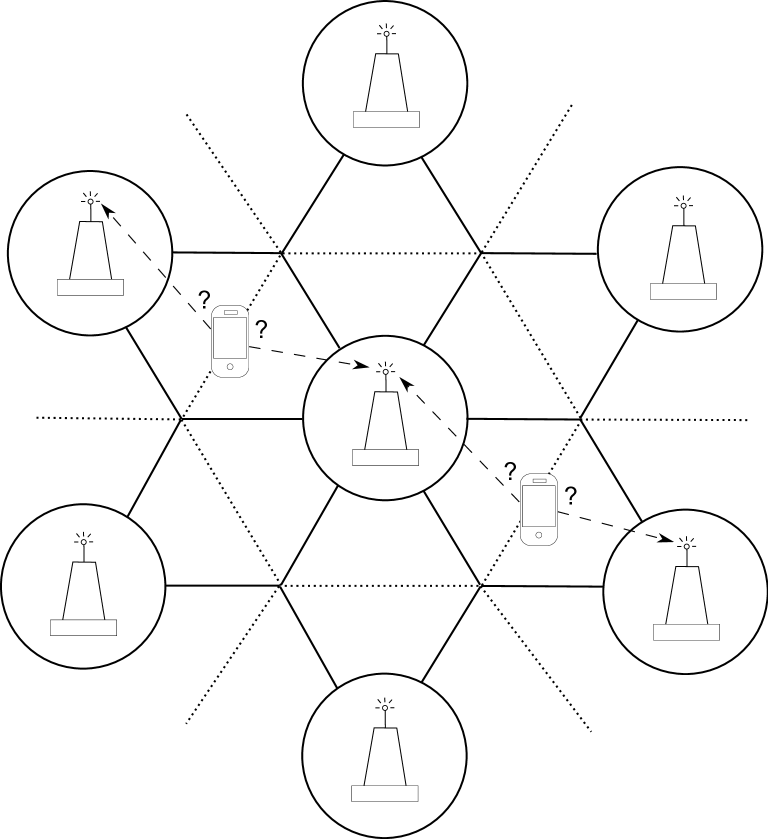
Figure 3: Association problem in the simplifed setting

V-B Results

We first compare the four policies given in the previous section. Figures 4 and 5 show the mean file transfer time and the outage probability for each policy, as a function of the served traffic. The reference policy is “best peak rate” where users simply connect to the base station offering the best peak rate (i.e the best SINR), without considering the loads of available BSs. The reference policy has the worst performance, since it is not load-aware, namely, it attaches users to the closest BS, even if it is overloaded, which does not reduce network congestion when traffic is high. Policy “smallest workload” brings little improvement, because, even though it takes the loads into account, it can possibly admit a user when the number of active users is already large, resulting in outage. Indeed, even for a large number of active users, the workload can be small if they have almost finished their transfer, or if their data rate is high. Policies “best data rate” and “shortest queue” perform the best, and bring large improvement in both outage probability and file transfer time. For high traffic, say $100$ Mbps, policies “best peak rate” and “smallest workload” yield a mean file transfer time of $7$ s and a outage probability of $60\%$. Policies “best data rate” and “shortest queue” yield $4$ s for the mean file transfer time and $10\%$ for the outage probability. This shows that reducing congestion has a considerable impact on the network performance.

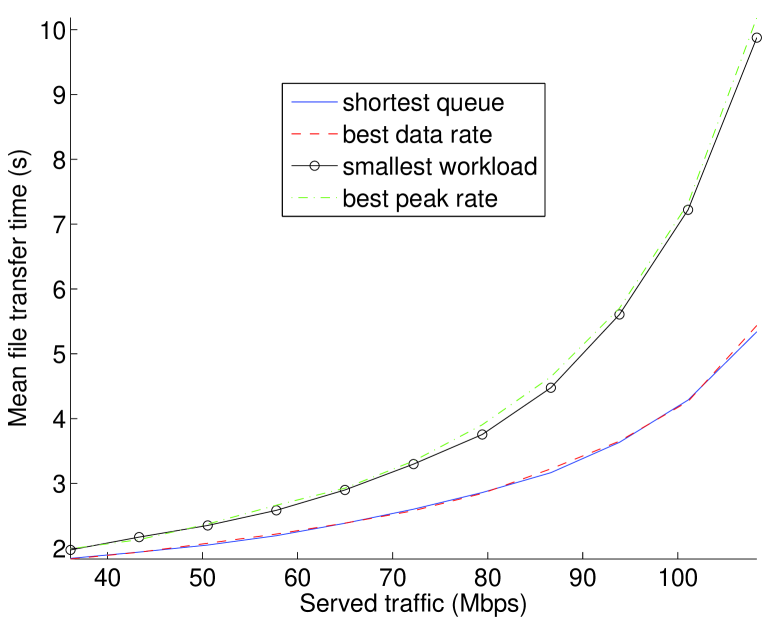
Figure 4: Mean file transfer time as a function of the served traffic

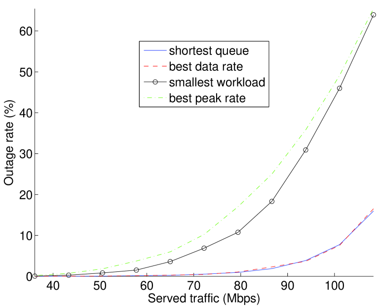
Figure 5: Outage probability as a function of the served traffic

Figure 6 shows the accuracy of the gradient estimates obtained using the policy gradient method (denoted “centralized” in the graphs) and the proposed heuristic which allows a distributed implementation (denoted “distributed”). We choose $\theta=0$ for our comparison. For a fixed number of time steps, we generate $500$ gradient estimates using both methods, and we calculate the sign of the dot product between the gradient estimate and the true gradient obtained by finite difference for a long simulation with $100,000$ time steps. If their dot product is strictly positive, then the gradient estimate is an admissible ascent direction. We plot the percentage of gradient estimates which are admissible ascent directions. The higher the percentage, the better the gradient estimate is. We can see that the accuracy of gradient estimates goes to $100\%$ when the number of time steps grows. We can also see that the proposed heuristic performs significantly better than the straighforward policy gradient. For the same level of accuracy (say $95\%$) the number of time steps required by the heuristic is $10$ times smaller than for the classical policy gradient.

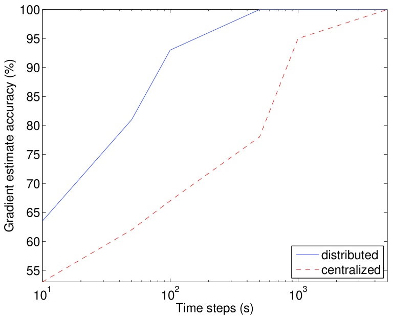
Figure 6: Accuracy of gradient estimates as a function of the number of time steps

Figure 7 and 8 show the evolution of the average cost and the corresponding controller parameter values. The total traffic is $100$ Mbps. Since the number of parameters is large ($57$ in total), only the two first components of the parameter vector are represented. For each update of $\theta$, the gradient is estimated during $100$ seconds. Starting from $\theta=0$, and a heavily congested network, the outage probability diminishes almost monotonically. This demonstrates that the algorithm is able to find a configuration of parameters for which the congestion in the network is reduced. The algorithm convergence speed with regards to the evolution of the daily traffic is satisfactory, since in operational networks, the traffic pattern (arrival rates in each region) can reasonably be assumed fixed for at least one hour.

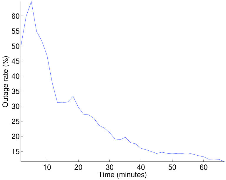
Figure 7: Average cost during the learning process

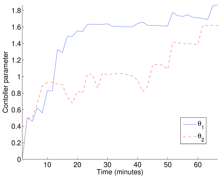
Figure 8: Controller parameters during the learning process

VI Conclusion

In this paper we have proposed a model for the association problem in wireless networks. This model takes into account traffic dynamics making it possible to optimize performance indicators directly perceived by users like the mean file transfer time and the outage probability. In the static framework, we show that the related association problem is tractable by classical convex optimization techniques and reduces to a routing problem. In the dynamic context, the association problem is modeled as a MDP. An on-line Policy Gradient Reinforcement Learning method has been proposed and adapted to the association problem to optimally control the system. A heuristic has been introduced to enable the algorithm to be implemented in a distributed manner, and improve the gradient estimation procedure dramatically. The approach has the following important advantages which make it suitable for practical implementation:

1. Its convergence to a local optimum can be proven mathematically

2. The average system performance improves monotonically, and convergence speed is compatible with typical traffic evolution in operational networks

3. The solution is scalable, since its complexity increases linearly with the number of BSs

4. The solution can be implemented in a distributed manner.

Numerical experiments have demonstrated that the proposed solution performs well in practice, and effectively decreases congestion in the network.

References

- [1] S. Horrich, S. Elayoubi, and S. Ben Jemaa, “On the impact of mobility and joint rrm policies on a cooperative wimax/hsdpa network,” in Wireless Communications and Networking Conference, 2008. WCNC 2008. IEEE, 31 2008-april 3 2008, pp. 2027 –2032.
- [2] S. Buljore, H. Harada, S. Filin, P. Houze, K. Tsagkaris, O. Holland, K. Nolte, T. Farnham, and V. Ivanov, “Architecture and enablers for optimized radio resource usage in heterogeneous wireless access networks: The ieee 1900.4 working group,” Communications Magazine, IEEE, vol. 47, no. 1, pp. 122 –129, january 2009.
- [3] M. Haddad, S. Elayoubi, E. Altman, and Z. Altman, “A hybrid approach for radio resource management in heterogeneous cognitive networks,” Selected Areas in Communications, IEEE Journal on, vol. 29, no. 4, pp. 831 –842, april 2011.
- [4] 3GPP, “Evolved Universal Terrestrial Radio Access (E-UTRA) and Evolved Universal Terrestrial Radio Access (E-UTRAN); Overall description; Stage 2,” 3rd Generation Partnership Project (3GPP), TS 36.300, Sep. 2008.
- [5] ——, “Evolved Universal Terrestrial Radio Access Network (E-UTRAN); Self-configuring and self-optimizing network (SON) use cases and solutions,” 3rd Generation Partnership Project (3GPP), TR 36.902, Sep. 2008. [Online]. Available: http://www.3gpp.org/ftp/Specs/html-info/36902.htm
- [6] R. Sutton and A. Barto, Reinforcement Learning, an Introduction. MIT Press, 1998.
- [7] M. L. Puterman, Markov Decision Processes: Discrete Stochastic Dynamic Programming. Wiley-Interscience, 2005.
- [8] R. J. Williams, “Simple statistical gradient-following algorithms for connectionist reinforcement learning,” Machine Learning, vol. 8, pp. 229–256, 1992, 10.1007/BF00992696. [Online]. Available: http://dx.doi.org/10.1007/BF00992696
- [9] J. Baxter and P. L. Bartlett, “Infinite-Horizon Policy-Gradient Estimation,” Journal of Artificial Intelligence Research, vol. 15, pp. 319–350, 2001. [Online]. Available: http://citeseerx.ist.psu.edu/viewdoc/summary?doi=10.1.1.21.8723
- [10] J. Baxter, P. L. Bartlett, and L. Weaver, “Experiments with Infinite-Horizon Policy-Gradient Estimation,” Journal of Artificial Intelligence Research, vol. 15, pp. 351–381, 2001. [Online]. Available: http://www.jair.org/papers/paper807.html
- [11] R. Combes, Z. Altman, and E. Altman, “Scheduling gain for frequency-selective rayleigh-fading channels with application to self-organizing packet scheduling,” Performance Evaluation, Feb. 2011.
- [12] ——, “A self-optimization method for coverage-capacity optimization in ofdma networks with mimo,” in Value Tools 2011.
- [13] R. Combes, S. E. Elayoubi, and Z. Altman, “Cross-layer analysis of scheduling gains: Application to lmmse receivers in frequency-selective rayleigh-fading channels,” in WiOpt 2011, 2011.
- [14] T. Bonald and A. Proutière, “Wireless downlink data channels: User performance and cell dimensioning,” in ACM Mobicom, 2003.
- [15] J. D. C. Little, “A Proof for the Queuing Formula: L= W,” Operations Research, vol. 9, no. 3, pp. 383–387, 1961. [Online]. Available: http://dx.doi.org/10.2307/167570
- [16] S. Boyd and L. Vandenberghe, Convex Optimization. Cambridge University Press, 2004.
- [17] D. Blackwell, “Discrete dynamic programming,” Annals of Mathematical Statistics, vol. 33, no. 2, pp. 719–726, 1962.