Space-Efficient Parallel Algorithms for Combinatorial Search Problems

Abstract

We present space-efficient parallel strategies for two fundamental combinatorial search problems, namely, backtrack search and branch-and-bound, both involving the visit of an $n$-node tree of height $h$ under the assumption that a node can be accessed only through its father or its children. For both problems we propose efficient algorithms that run on a $p$-processor distributed-memory machine. For backtrack search, we give a deterministic algorithm running in ${O}\left(n/p+h\log p\right)$ time, and a Las Vegas algorithm requiring optimal ${O}\left(n/p+h\right)$ time, with high probability. Building on the backtrack search algorithm, we also derive a Las Vegas algorithm for branch-and-bound which runs in ${O}\left((n/p+h\log p\log n)h\log^{2}n\right)$ time, with high probability. A remarkable feature of our algorithms is the use of only constant space per processor, which constitutes a significant improvement upon previous algorithms whose space requirements per processor depend on the (possibly huge) tree to be explored.

Introduction

The exact solution of a combinatorial (optimization) problem is often computed through the systematic exploration of a tree-structured solution space, where internal nodes correspond to partial solutions (growing progressively more refined as the depth increases) and leaves correspond to feasible solutions. A suitable algorithmic template used to study this type of problems (originally proposed in [2]) is the exploration of a tree $\mathcal{T}$ under the constraints that: (i) only the tree root is initially known; (ii) the structure, size and height of the tree are unknown; and (iii) a tree node can be accessed if it is the root of the tree or if either its father or one of its children is available.

In the paper, we focus on two important instantiations of the above template. The backtrack search problem [3] requires to explore the entire tree $\mathcal{T}$ starting from its root $r$, so to enumerate all solutions corresponding to the leaves. In the branch-and-bound problem, each tree node is associated to a cost, and costs satisfy the min-heap order property, so that the cost of an internal node is a lower bound to the cost of the solutions corresponding to the leaves of its subtree. The objective here is to determine the leaf associated with the solution of minimum cost. We define $n$ and $h$ to be, respectively, the number of nodes and the height of the tree to be explored. It is important to remark that in the branch-and-bound problem, the nodes that must necessarily be explored are only those whose cost is less than or equal to the cost of the solution to be determined. These nodes form a subtree $\mathcal{T}^{*}$ of $\mathcal{T}$ and in this case $n$ and $h$ refer to $\mathcal{T}^{*}$. Assuming that a node is explored in constant time, it is easy to see that the solution to the above problems requires ${\Omega}\left(n\right)$ time, on a sequential machine, and ${\Omega}\left(n/p+h\right)$ time on a $p$-processor parallel machine.

Due to the elevated computational requirements of search problems, many parallel algorithms have been proposed in literature that speed-up the execution by evenly distributing the computation among the available processing units. All these studies have focused mainly on reducing the running time while the resulting memory requirements (expressed as a function of the number of nodes to be stored locally at each processor) may depend on the tree parameters. However, the search space of combinatorial problems can be huge, hence it is fundamental to design algorithms which exploit parallelism to speed up execution and yet need a small amount of memory per processor, possibly independent of the tree parameters. Reducing space requirements allows for a better exploitation of the memory hierarchy and enables the use of cheap distributed-memory parallel platforms where each processing units is endowed with limited memory.

Previous work

Parallel algorithms for backtrack search have been studied in a number of different parallel models. Randomized algorithms have been developed for the complete network [3, 4] and the butterfly network [5], which require optimal ${\Theta}\left(n/p+h\right)$ node explorations (ignoring the overhead due to manipulations of local data structures). The work of Herley et al. [6] gives a deterministic algorithm running in ${O}\left((n/p+h)(\log\log\log p)^{2}\right)$ time on a $p$-processor COMMON CRCW PRAM. While the algorithm in [3] performs depth-first explorations of subtrees locally at each processor requiring ${\Omega}\left(h\right)$ space per processor, the other algorithms mostly concentrate on balancing the load of node explorations among the available processors but may require ${\Omega}\left(n/p\right)$ space per processor.

In [3] an ${\Theta}\left(n/p+h\right)$-time randomized algorithm for branch-and-bound is also provided for the complete network. In [7, 8] Herley et al. show that a parallelization of the heap-selection algorithm of [9] gives, respectively, a deterministic algorithm running in time ${O}\left(n/p+h\log^{2}(np)\right)$ on an EREW-PRAM, and one running in time ${O}\left((n/p+h\log^{4}p)\log\log p\right)$ on the Optically Connected Parallel Computer (OCPC), a weak variant of the complete network [10]. All of these works adopt a best-first like strategy, hence they may need ${\Omega}\left(n/p\right)$ space per processor. In [11] deterministic algorithms for both backtrack search and branch-and-bound are given which run in ${O}\left(\sqrt{nh}\log n\right)$ time on an $n$-node mesh with constant space per processor. However, any straightforward implementation of these algorithms on a $p$-processor machine, with $p<n$, would still require ${\Omega}\left(n/p\right)$ space per processor. Karp et al. [2] describe sequential algorithms for the branch-and-bound problem featuring a range of space-time tradeoffs. The minimum space they attain is ${O}\left(\sqrt{\log n}\right)$ in time ${O}\left(n2^{O(\sqrt{\log n})}\right)$. Some papers (see [12] and references therein) describe sequential and parallel algorithms for branch-and-bound with limited space, which interleave depth-first and breadth-first strategies, but provide no analytical guarantee on the running time.

Our Contribution

In this paper, we present space-efficient parallel algorithms for the backtrack search and branch-and-bound problems. The algorithms are designed for a $p$-processor distributed-memory message-passing system similar to the one employed in [3], where in one time step each processor can perform ${O}\left(1\right)$ local operations and send/receive a message of ${O}\left(1\right)$ words to/from another arbitrary processor. In case two or more messages are sent to the same processor in one step, we make the restrictive assumption that none of these messages is delivered (as in the OCPC model [10, 13]). Consistently with most previous works, we assume that a memory word is sufficient to store a tree node, and, as in [2], we also assume that, given a tree node, a processor can generate any one of its children or its father in ${O}\left(1\right)$ steps and ${O}\left(1\right)$ space.

For the backtrack search problem we develop a deterministic algorithm which runs in ${O}\left(n/p+h\log p\right)$ time, and a Las Vegas randomized algorithm which runs in optimal ${\Theta}\left(n/p+h\right)$ time with high probability, if $p={O}\left(n/\log n\right)$. Both algorithms require only constant space per processor and are based on a nontrivial lazy implementation of the work-distribution strategy featured in the backtrack search algorithm by [3], whose exact implementation requires ${\Omega}\left(h\right)$ space per processor. By using the deterministic backtrack search algorithm as a subroutine, we develop a Las Vegas randomized algorithm for the branch-and-bound problem which runs in ${O}\left((n/p+h\log p\log n)h\log^{2}n\right)$ time with high probability, using again constant space per processor.

To the best of our knowledge, our backtrack search algorithms are the first to achieve (quasi) optimal time using constant space per processor, which constitutes a significant improvement upon the aforementioned previous works. As for the branch-and-bound algorithm, while its running time may deviate substantially from the trivial lower bound, for search spaces not too deep and sufficiently high parallelism, it achieves sublinear time using constant space per processor. For instance, if $h={O}\left(n^{\epsilon}\right)$ and $p={\Theta}\left(n^{1-\epsilon}\right)$, with $0<\epsilon<1/2$, the algorithm runs in ${O}\left(n^{2\epsilon}\mbox{polylog}(n)\right)$ time, with high probability, using ${\Theta}\left(n^{1-\epsilon}\right)$ aggregate space. Again, to the best of our knowledge, ours is the first algorithm achieving sublinear running time using sublinear (aggregate) space, thus providing important evidence that branch-and-bound can be parallelized in a space-efficient way.

For simplicity, our results are presented assuming that the tree $\mathcal{T}$ to be explored is binary and that each internal node has both left and right children. The same results extend to the case of $d$-ary trees, with $d={\Theta}\left(1\right)$, and to trees that allow an internal node to have only one child.

The rest of the paper is organized as follows. In Section Space-Efficient Backtrack Search we first present a generic strategy for parallel backtrack search and then instantiate this strategy to derive our deterministic and randomized algorithms. In Section Space-Efficient Branch-and-Bound we describe the randomized parallel algorithm for branch-and-bound. In Section Conclusions we give some final remarks and indicate some interesting open problems.

Space-Efficient Backtrack Search

In this section we describe two parallel algorithms, a deterministic algorithm and a Las Vegas randomized algorithm, for the backtrack search problem. Both algorithms implement the same strategy described in Subsection Generic Strategy below and require constant space per processor. The deterministic implementation of the generic strategy (Section Deterministic Algorithm) requires global synchronization, while the randomized one (Section Randomized Algorithm) avoids explicit global synchronization. In the rest of the paper, we let $P_{0},P_{1},\ldots,P_{p-1}$ denote the processors in our system.

Generic Strategy

The main idea behind our generic strategy moves along the same lines as the backtrack search algorithm of [3], where at each time a processor is either idle or busy exploring a certain subtree of $\mathcal{T}$ in a depth-first fashion. The computation evolves as a sequence of epochs, where each epoch consists of three consecutive phases of fixed durations: (1) a traversal phase, where each busy processor continues the depth-first exploration of its assigned subtree; (2) a pairing phase, where some busy processors are matched with distinct idle processors; and (3) a donation phase, where each busy processor $P_{i}$ that was paired with an idle processor $P_{j}$ in the preceding phase, attempts to entrust a portion of its assigned subtree to $P_{j}$, which becomes in charge of the exploration of this portion.

In [3] it is shown that the best progress towards completion is achieved by letting a busy processor donate the topmost unexplored right subtree of the subtree which the processor is currently exploring. A straightforward implementation of this donation rule requires that a busy processor either stores a list of up to ${\Theta}\left(h\right)$ nodes, or, at each donation, traverses up to ${\Theta}\left(h\right)$ nodes in order to retrieve the subtree to be donated, thus incurring a large time overhead. As anticipated in the introduction, our algorithm features a lazy implementation of this strategy which uses constant space per processor but incurs only a small time overhead.

We now describe in more detail how the three phases of an epoch are performed. At any time, a busy processor $P_{i}$ maintains the following information, which can be stored in constant space:

• $r_{i}$: the root of its assigned subtree;

• $v_{i}$: the next node to be touched by the processor in the depth-first exploration of its assigned subtree;

• $d_{i}\in\{\mathtt{left},\mathtt{right},\mathtt{parent}\}$: a direction flag identifying the direction where the exploration must continue after touching $v_{i}$.

• $(t_{i},q_{i})$: a pair of nodes that are used to identify a portion of the subtree to donate to an idle processor; in particular, $t_{i}$ is a node on the path from $r_{i}$ to $v_{i}$, while $q_{i}$ is either the right child of $r_{i}$ or is undefined. We refer to the path from $t_{i}$ up to $r_{i}$ as the tail associated with processor $P_{i}$, and define the tail’s length as the number of edges it comprises.

At the beginning of the first epoch, only processor $P_{0}$ is busy and its variables are initialized as follows: $r_{0}$ is set to the root of the tree $\mathcal{T}$ to be explored; $v_{0}=t_{0}=r_{0}$; $q_{0}$ is set to the right child of $r_{0}$; and $d_{0}=\mathtt{left}$. Consider now an arbitrary epoch, and let $\Delta_{\mathrm{t}}$, $\Delta_{\mathrm{p}}$, and $\Delta_{\mathrm{d}}$ denote suitable values which will be fixed by the analysis.

Traversal phase

Each busy processor $P_{i}$ advances of at most $\Delta_{\mathrm{t}}$ steps in the depth-first exploration of the subtree rooted at $r_{i}$, starting from $v_{i}$ and proceeding in the direction indicated by $d_{i}$. Variables $v_{i}$ and $d_{i}$ are updated straightforwardly at each step, in accordance with the depth-first exploration sequence. In some cases, $r_{i}$ and $t_{i}$ must also be updated. In particular, $r_{i}$ is updated when $v_{i}=r_{i}$ and $d_{i}=\mathtt{right}$. In this case, denoting by $w$ the right child of $r_{i}$, in the next step both $r_{i}$ and $v_{i}$ are set to $w$, $d_{i}$ to $\mathtt{left}$, and $q_{i}$ to $w$’s right child. Instead, $t_{i}$ is updated when $v_{i}=t_{i}$ and $d_{i}=\mathtt{parent}$. In this case, in the next step both $t_{i}$ and $v_{i}$ are set to $v_{i}$’s parent. Also, $t_{i}$ is updated when $t_{i}=r_{i}$ and $r_{i}$ is updated. In this case $t_{i}$ is set always to the new value of $r_{i}$. $P_{i}$ finishes the exploration of its assigned subtree and becomes idle after touching $v_{i}$ with $v_{i}=r_{i}$ and $d_{i}=\mathtt{parent}$.

Pairing phase

Busy and idle processors are paired in preparation of the subsequent donation phase. The phase runs for $\Delta_{\mathrm{p}}$ steps. Different pairing mechanisms are employed by the deterministic and the randomized algorithm, as described in detail in the respective sections.

Donation phase

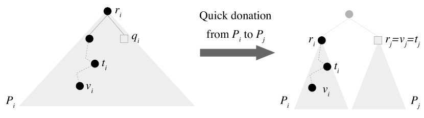
Figure 1: Example of quick donation. Subtrees are denoted by shaded area and the processors in charge of their explorations, before and after the donation, are indicated at the bottom. Grey circles denote nodes that will not be touched again; black circles denote nodes have already been touched but will be touched again; and squares denote nodes that have not been touched yet.

Consider a busy processor $P_{i}$ that has been paired to an idle processor $P_{j}$. Two types of donations from $P_{i}$ to $P_{j}$ are possible, namely a quick donation or a slow donation, depending on the status of $q_{i}$. As we will see, a quick donation always starts and terminates within the same epoch, assigning a subtree to explore to $P_{j}$, while a slow donation may span several epochs and may even fail to assign a subtree to $P_{j}$.

If $q_{i}$ is defined, hence, it is the right child of $r_{i}$, a quick donation occurs (see Figure 1). In this case, $P_{i}$ donates to $P_{j}$ the subtree rooted in $q_{i}$ and $P_{i}$ keeps the subtree rooted at the left child of $r_{i}$ for exploration. Thus, $P_{j}$ sets $r_{j},v_{j}$ and $t_{j}$ all equal to $q_{i}$. If $q_{i}$ is a leaf, then $P_{j}$ sets $d_{j}$ to $\mathtt{parent}$ and $q_{j}$ to undefined, otherwise it sets $q_{j}$ to the right child of $q_{i}$ and $d_{j}$ to $\mathtt{left}$. Instead, $P_{i}$ sets $r_{i}$ to $r_{i}$’s left child and $q_{i}$ to undefined, while $v_{i}$ and $d_{i}$ remain unchanged. Also, if $t_{i}$ was equal to $r_{i}$ it is reset to the new value of $r_{i}$, otherwise it remains unchanged. (Note that quick donation coincides with the donation strategy in [3]).

If $q_{i}$ is undefined, a slow donation is performed where the tail associated with $P_{i}$ is climbed upwards to identify an unexplored subtree which is then donated to $P_{j}$. To amortize the cost of tail climbing, $P_{i}$ attempts to donate a subtree rooted at a node located in the middle of the tail, so to halve the length of the residual tail that $P_{i}$ has to climb in future slow donations. This halving is crucial for reducing the running time.

Let us see in more detail how a slow donation is accomplished. Initially, $P_{i}$ verifies if a new tail must be created. This happens if $t_{i}=r_{i}$. In this case, a tail creation is performed by setting $t_{i}=v_{i}$. Then, two cases are possible depending on the tail length.

Case 1: tail length $\mathbf{\leq 1}$. Suppose that the tail length is 0, that is, $t_{i}=v_{i}=r_{i}$. Because of the way $r_{i}$ is updated in the traversal phase, it can be easily seen that in this case $d_{i}=\mathtt{right}$, since otherwise $q_{i}$ would be defined. Hence $P_{i}$ must have already fully explored the left subtree of $r_{i}$. Analogously, the left subtree of $r_{i}$ has been fully explored by $P_{i}$ if $t_{i}$ is the right child of $r_{i}$ (tail length 1). In both cases, no donation is performed and, since the current root is no longer needed, $P_{i}$ sets $r_{i},v_{i}$ and $t_{i}$ to the right child of $r_{i}$, and $d_{i}$ to $\mathtt{left}$. If instead, $t_{i}$ is the left child of $r_{i}$ (tail length 1), then $P_{i}$ donates to $P_{j}$ the subtree rooted at the right child of $r_{i}$, performing the same steps of a quick donation. Note that in all cases, the level of the root of the subtree assigned to $P_{i}$ increases by 1.

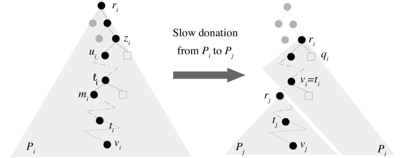
Figure 2: Example of slow donation when the tail length is larger than 1. The tail is the path from $r_{i}$ to $t_{i}$. Node $u_{i}$ is the left child closest to $r_{i}$ along the tail. Subtrees are denoted by shaded area and the processors in charge of their explorations, before and after the donation, are indicated at the bottom. Grey circles denote nodes that will not be touched again; black circles denote nodes have already been touched but will be touched again; and squares denote nodes that have not been touched yet.

Case 2: tail length $\mathbf{>1}$. First, processor $P_{i}$ identifies the middle node $m_{i}$ of the tail by backtracking twice from $t_{i}$ to $r_{i}$. Then $P_{i}$ donates to $P_{j}$ the (partially explored) subtree rooted at $m_{i}$, and $P_{j}$ sets $r_{j}=m_{i}$, $v_{j}=v_{i}$, $d_{j}=d_{i}$, $t_{j}=t_{i}$, and sets $q_{j}$ to undefined. While backtracking to identify $m_{i}$, $P_{i}$ seeks the node $u_{i}$ along the path from $m_{i}$ to $r_{i}$ which is closest to $r_{i}$ and is the left child of its parent $z_{i}$. If such a node does not exist, then $P_{i}$ becomes idle since only the exploration of the subtree donated to $P_{j}$ needed completion. If instead, $u_{i}$ is identified, all nodes in the path from its parent $z_{i}$ (excluded) to $r_{i}$ (included) are unnecessary to complete the exploration of the subtree rooted at $r_{i}$, since they and their left subtrees have already been explored. Therefore $P_{i}$ continues the exploration by setting $r_{i}$to $z_{i}$, $q_{i}$ to the right child of $z_{i}$, and both $v_{i}$ and $t_{i}$ to the parent $\ell_{i}$ of $m_{i}$. Also, $d_{i}$ is set to $\mathtt{right}$ if $m_{i}$ is the left child of $\ell_{i}$, or to $\mathtt{parent}$ otherwise. This case of slow donation is depicted in Figure 2. Note that the level of the root of the subtree assigned to $P_{j}$ is always greater than the level of the root of the subtree assigned to $P_{i}$. Moreover, the level of the root of the subtree assigned to $P_{i}$ either increases or remains unchanged. In this latter case, however, $q_{i}$ can be set during the tail traversal so that the next donation of $P_{i}$ will be a quick donation.

The donation phase runs for $\Delta_{\mathrm{d}}$ steps, where we assume $\Delta_{\mathrm{d}}$ to be greater than or equal to the maximum between the time for a quick donation and the time for Case 1 of a slow donation. However, for efficiency reasons, $\Delta_{\mathrm{d}}$ cannot be chosen large enough to perform entirely Case 2 of a slow donation, since its duration is proportional to the tail length, which may be rather large. In this case, if $P_{i}$ does not conclude the donation in $\Delta_{\mathrm{d}}$ steps, it saves its state (requiring constant space) at the end of the donation phase and resumes the computation in the donation phase of the subsequent epoch, in which it maintains the pairing with $P_{j}$ and refuses any further pairing. If $t_{i}$ changes in the subsequent traversal phase, the state is updated accordingly: namely, if $t_{i}$ is set to its father, the tail length is updated and, if needed, $m_{i}$ is moved to its father to ensure that it remains as the middle node between $t_{i}$ and $r_{i}$. Also, if the tail length becomes at most one, the slow donation switches from Case 2 to Case 1.

It is easy to check that the above algorithms touches all the nodes in the tree ${\mathcal{T}}$, therefore solving the backtrack search problem.

Deterministic Algorithm

In the deterministic algorithm each pairing phase is performed through a prefix-like computation that finds a maximal matching between idle processors and busy processors; such computation requires ${\Theta}\left(\log p\right)$ parallel time. For this algorithm we set $\Delta_{\mathrm{p}},\Delta_{\mathrm{d}}={\Theta}\left(\log p\right)$, and $\Delta_{\mathrm{t}}=\Delta_{\mathrm{d}}/\kappa$, for a suitable constant $\kappa$ defined in the proof. We call an epoch full if in the last step of its traversal phase at least $p/2$ processors are busy, and we call it non-full otherwise.

Lemma 1

The total number of parallel steps in full epochs is ${O}\left(n/p\right)$.

Proof

Since each node is touched at most 3 times in a traversal phase (after descending from the parent, after exploring the left subtree, and after exploring the right subtree), the total number of times nodes are touched is ${O}\left(n\right)$. The lemma follows by observing that in a full epoch ${\Theta}\left(p\right)$ processors touch ${\Theta}\left(\log p\right)$ nodes each, and that the epoch runs in ${O}\left(\log p\right)$ parallel steps.

Consider an arbitrary node $q$ of ${\mathcal{T}}$. Now, we bound the number of parallel steps in non-full epochs before $q$ is touched. Observe that after all leaves have been touched, the algorithm terminates in ${O}\left(h+\log p\right)$ additional parallel steps, when all busy processors have gone back to the roots of their assigned subtrees. In each epoch, we define the special processor of $q$ as the processor exploring the subtree containing $q$ with the deepest root; note that there is a unique special processor in any epoch. When the special processor $S$ performs a donation to a processor $P_{j}$, then for the subsequent epoch either $S$ remains the special processor or $P_{j}$ becomes the special processor. We denote with $\mathcal{T}_{q}$ the subtree of $\mathcal{T}$ containing nodes not larger than $q$, and with $n_{q}$ and $h_{q}$ its size and height.

We refer to non-full epochs as donating or preparing depending on the status of the special processor of $q$. Namely, a non-full epoch is donating if the special processor $S$ completes a donation in the epoch, while it is preparing if $S$ is involved in Case 2 of a slow donation and, at the end of the epoch, it has not finished to execute all operations prescribed by this type of donation. Note that, before $q$ is touched, any non-full epoch is always either donating or preparing.

Lemma 2

The total number of parallel steps in donating epochs before node $q$ is touched is ${O}\left(h_{q}\log p\right)$.

Proof

We claim that the level of the root of the subtree explored by special processor $S$ increases by at least one after at most two donating epochs. If a quick donation, or Case 1 of slow donation is performed by $S$, then the claim is verified. Suppose $S$ is involved in Case 2 of a slow donation. Let $S=P_{i}$ and let $P_{j}$ be the processor paired to $P_{i}$. If after the donation $P_{i}$ remains the special processor and the root $r_{i}$ of its subtree is unchanged, then during the slow donation $q_{i}$ has been set and hence the next donation of the special processor is a quick donation. In all other cases, the level root of the special processor is increased after the donation. Thus, the claim is proved. Since the height of $\mathcal{T}_{q}$ is $h_{q}$, there are ${O}\left(h_{q}\right)$ donating epochs and the total number of parallel steps in donating epochs is ${O}\left(h_{q}\log p\right)$.

We now bound the total number of parallel steps in preparing epochs. This number is function of the number $E_{q}$ of parallel steps in full epochs before $q$ is touched. We observe that $E_{q}$ depends on $q$ but also on the the size and height of tree $\mathcal{T}$ (we do not represent this dependency for notational simplicity).

Lemma 3

Let $E_{q}$ be the number of steps in full epochs before node $q$ is touched. Then, the total number of parallel steps in preparing epochs before node $q$ is touched is ${O}\left(E_{q}+h_{q}\log p\right)$.

Proof

Consider the time interval from the beginning of the algorithm until leaf $q$ is explored. Clearly, at any time within this interval a special processor is defined. We partition this interval into eras delimited by subsequent donation phases in which tail creations are performed by the special processor. (Recall that a processor $P_{i}$ creates a tail in the donation phase of an epoch whenever $q_{i}$ is undefined, $t_{i}=r_{i}$ and $v_{i}\neq r_{i}$: then the tail is created by setting $t_{i}=v_{i}$.) More precisely, for $i\geq 1$, the $i$-th era begins at the donation phase of the $i$-th tail creation, and ends right before the donation phase of the $(i+1)$-st tail creation (or the end of the interval). Observe that the beginning of the interval does not coincide with the beginning of the first era, however no preparing epochs occur before the first tail creation. Note that an era may involve more than one donation from the special processor, and that all preparing epochs in the same era work on segments of the tail whose creation defines the beginning of the era. We denote with $\Phi$ the number of eras and with $\phi_{i}\geq 1$ the number of slow donations in the $i$-th era, for each $1\leq i\leq\Phi$ .

Let $T_{i}^{j}$ be the number of distinct nodes that the special processor touches by walking up a subtree to prepare the $j$-th slow donation of the $i$-th era, with $1\leq i\leq\Phi$ and $1\leq j\leq\phi_{i}$ (nodes can be touched in both donating and preparing epochs). Since a slow donation splits the tail in half, we have that $T_{i}^{j+1}\leq{T_{i}^{j}}/{2}$ for all $1\leq j\leq\phi_{i}$. Since the number of steps in preparing epochs for one slow donation is at most proportional to the tail length, the total time spent in preparing epochs is $\sum_{i=1}^{\Phi}\sum_{j=1}^{\phi_{i}}cT_{i}^{j}\leq 2c\sum_{i=1}^{\Phi}T_{i}^{1}$, where $c\geq 1$ is a suitable constant. We have $T_{1}^{1}\leq E_{q}+{O}\left(\log p\right)$ since the first era starts, in the worst case, after all full epochs and after the traversal phase of the first non-full epoch (since the special processor always receives a donation request in the first non-full epoch).

Consider an arbitrary era $i\geq 2$. A node $u$ in the tail of the era has been touched for the first time in a traversal phase of an era $\ell<i$. Note that $\ell=i-1$ since if it was $\ell<i-1$, $u$ would have been part of a tail created in an era before the $i$-th one and it is easy to verify that tails of different eras are disjoint. Therefore the number of nodes touched by the special processor (walking upwards in the tree) in the preparing epochs for the first donation of era $i$ is bounded by the number of nodes touched by the special processor in the traversal phases of era $i-1$, which can be partitioned in three (disjoint) sets:

• the nodes touched for the first time in traversal phases of full epochs in era $i-1$; we denote the number of such nodes as $E_{i}$;

• the nodes touched for the first time in the traversal phases of donating epochs in era $i-1$; we denote the number of such nodes as $D_{i}$;

• the nodes touched for the first time in the traversal phases of preparing epochs in era $i-1$; we denote the number of such nodes as $C_{i}$.

Thus we have $\sum_{i=2}^{\Phi}T_{i}^{1}\leq\sum_{i=2}^{\Phi}E_{i}+\sum_{i=2}^{\Phi}D_{i}+\sum_{i=2}^{\Phi}C_{i}$. By assumption we have $\sum_{i=2}^{\Phi}E_{i}=E_{q}$, while by Lemma 2 it follows that $\sum_{i=2}^{\Phi}D_{i}={O}\left(h_{q}\log p\right)$. We now only need to bound $\sum_{i=2}^{\Phi}C_{i}$. Remember that $C_{i}$ is the number of nodes touched in the preparing epochs of the $i$-th era that have been touched for the first time in the traversal phases of preparing epochs of the $(i-1)$-st era. Consider the second era: in order to bound $C_{2}$, we need to bound the number of nodes that have been touched in the traversal phases of epochs in the first era. Since $cT_{1}^{j}$ is an upper bound to the time required for preparing the $j$-th donation in the first era, and since the number of nodes visited in the traversal phase of a preparing epoch is at most a factor $1/\kappa$ the time of the respective donation phase, for a suitable constant $\kappa$ (i.e., $\Delta_{\mathrm{t}}=\Delta_{\mathrm{d}}/\kappa$), we have $C_{2}\leq\sum_{j=1}^{\phi_{i}}cT_{1}^{j}/\kappa\leq T_{1}^{1}/2$ by setting $\kappa=2c$. In general, for era $i>2$ we have: $C_{i}\leq\sum_{j=1}^{\phi_{i}}{cT_{i-1}^{j}}/{\kappa}\leq{T_{i-1}^{1}}/{2}\leq(E_{i-1}+D_{i-1}+C_{i-1})/2$. Then, by unfolding the above recurrence, we get

$$C_{i}\leq\frac{1}{2}E_{i-1}+\frac{1}{4}E_{i-2}+\dots+\frac{1}{2^{i-2}}E_{2}+\frac{1}{2}D_{i-1}+\frac{1}{4}D_{i-2}+\dots+\frac{1}{2^{i-2}}D_{2}+\frac{1}{2^{i-1}}T_{1}^{1}.$$

Therefore, by summing up among all eras, we have

$$\sum_{i=2}^{\Phi}C_{i}\leq\sum_{i=1}^{\Phi}\left[\frac{T_{1}^{1}}{2^{i}}+\sum_{j=1}^{\infty}\frac{E_{i}}{2^{j}}+\sum_{j=1}^{\infty}\frac{D_{i}}{2^{j}}\right]\leq T_{1}^{1}+\sum_{i=1}^{\Phi}\left(E_{i}+D_{i}\right)={O}\left(E_{q}+h_{q}\log p\right).$$

As already noticed, the number of steps in preparing epochs is proportional to the number of nodes touched in such epochs, and this establishes the result.

By combining the above three lemmas, we obtain the following theorem.

Theorem 0.1

The deterministic algorithm for backtrack search completes in ${O}\left(n/p+h\log p\right)$ parallel steps and constant space per processor.

Proof

By Lemma 1, there are at most ${O}\left(n/p\right)$ steps in full epochs. Then, by Lemma 2 and Lemma 3 (with $E_{q}={O}\left(n/p\right)$), we have that all nodes in $\mathcal{T}$ are touched after ${O}\left(n/p+h\log p\right)$ steps. Let $q$ be the last touched leaf. After ${O}\left(h\right)$ steps the processor $P_{i}$ that have touched $q$ reaches the root $r_{i}$ and becomes idle since the respective subtree has been completely explored, and after ${O}\left(\log p\right)$ steps all processors recognize the entire tree $\mathcal{T}$ have been explored and the algorithm ends. Since each processor stores a constant number of words and nodes, the theorem follows.

Randomized Algorithm

In the randomized algorithm, the durations of the traversal and of the pairing phase are set to a constant (i.e., $\Delta_{\mathrm{d}},\Delta_{\mathrm{p}}={O}\left(1\right)$), and the duration of a donation phase is set to $\Delta_{\mathrm{t}}=\Delta_{\mathrm{d}}/\kappa$, for a suitable constant $\kappa$. While the traversal phase and the donation phase are as described in section Generic Strategy and are the same as in the deterministic algorithm, the pairing phase is implemented differently as follows. In a first step, each idle processor sends a pairing request to a random processor; in a second step, a busy processor $P_{i}$ that has received a pairing request from (idle) processor $P_{j}$, sends a message to $P_{j}$ to establish the pairing. Note that the communication model described in Introduction (Our Contribution) guarantees that each busy processor receives at most one pairing request in the first step. The analysis of the randomized algorithm combines elements of the analysis of the above deterministic algorithm and the one for the randomized backtrack search algorithm in [3].

Theorem 0.2

The randomized algorithm completes in ${O}\left({n}/{p}+h\right)$ parallel steps with probability at least $1-n^{-c}$ for any constant $c>0$.

Proof

The analysis of the randomized algorithm combines elements of the analysis of the deterministic algorithm, presented in section Deterministic Algorithm, and the one by Karp and Zhang for their randomized backtrack search algorithm [3]. Differently from the deterministic algorithm, we define an epoch full if there are at least $p/4$ busy processors at the end of the traversal phase, and non-full otherwise. Reasoning as in Lemma 1, we have that the number of steps in full epochs is ${O}\left({n}/{p}\right)$. Consider now non-full epochs and an arbitrary leaf $q$ of $\mathcal{T}$, and classify such epochs as donating or preparing with respect to the special (busy) processor $S$ for $q$. Note that due to the randomized pairing, a non-full epoch can be both non-donating and non-preparing with respect to $S$, since we are not guaranteed that in non-full epochs processor $S$ is contacted by an idle processor. We call such (non-donating and non-preparing) non-full epochs waiting with respect to $S$. Reasoning as in Lemma 2, we have that after ${O}\left(h\right)$ donating epochs $q$ is touched, hence the number of steps in donating epochs is ${O}\left(h\right)$ (recall that each epoch comprises a constant number of steps). Also, using the same argument of Lemma 3, it can be proved that the total number of steps in preparing epochs is ${O}\left(n/p+h\right)$.

Finally, we upper bound the number of steps in waiting epochs by showing that for any leaf $q$, the number of waiting epochs before $q$ is touched is greater than $15d(n/p+h)$, for a suitable constant $d\geq 1$, with probability at most $e^{-n/(4p)}$. Consider a non-full epoch where the special processor can initiate a donation since it does not need to complete a previously started donation. Since in a non-full epoch the number of busy processors is $<p/4$, the number $\hat{p}$ of idle processors that are not waiting for the completion of donations started in earlier epochs is at least $p/2$. Therefore the probability that the special processor is paired to exactly one idle processor and the epoch is donating or preparing is ${\hat{p}\choose 1}(1/p)(1-1/p)^{\hat{p}-1}\geq 1/8$. Consider now a non-full epoch where the special processor resumes a previously interrupted donation. In this case the probability of being donating or preparing is one. Thus, the probability that a non-full epoch is donating or preparing is at least $1/8$, while the probability an epoch is waiting is at most $7/8$.

Let $\mathcal{B}(k,N,\rho)$ denote the probability that there are less than $k$ successes in $N$ independent Bernoulli trials, where each trial has probability $\rho$ of success. As shown above, after at most $d(n/p+h)$ donating and preparing epochs, for a suitable constant $d\geq 1$, leaf $q$ is touched. Thus, the probability of having more than $15d(n/p+h)$ waiting epochs is bounded above by $\mathcal{B}(d(n/p+h),16d(n/p+h),1/8)$. By a Chernoff bound [14] we have that $\mathcal{B}(d(n/p+h),16d(n/p+h),1/8)\leq e^{-d(n/p+h)/4}\leq e^{-(d\log n)/4}$ since $h\geq\log n$. Then, since a waiting epoch lasts ${O}\left(1\right)$ steps, $q$ is touched after ${O}\left(n/p+h\right)$ steps. By the union bound, the probability that each leaf is touched in ${O}\left(n/p+h\right)$ steps is $\leq ne^{-(d\log n)/4}\leq n^{-c}$ by setting $d$ larger than $4(c+1)/\log e$. The theorem follows.

Space-Efficient Branch-and-Bound

In this section we present a Las Vegas algorithm for the branch-and-bound problem, which requires to explore a heap-ordered binary tree $\mathcal{T}$, starting from the root, to find the minimum-cost leaf. For simplicity, we assume that all node costs are distinct. The algorithm implements, in a parallel setting, an adaptation of the sequential space-efficient strategy proposed in [2], which reduces the branch-and-bound problem to the problem of finding the node with the $n$-th smallest cost, for exponentially increasing values of $n$. In what follows, we first present an algorithm for a generalized selection problem, which uses the deterministic backtrack algorithm from the previous section as a subroutine. The generalization aims at controlling also the height of the explored subtrees which, in some cases, may dominate the parallel complexity. Then, we show how to reduce branch-and-bound to the generalized selection problem.

Generalized Selection

Let $\mathcal{T}$ be an infinite binary tree whose nodes are associated with distinct costs satisfying the min-heap order property, and let $c(u)$ denote the cost associated with a node $u$. We use $\mathcal{T}_{c}$ to denote the subtree of $\mathcal{T}$ containing all nodes of cost less than or equal to a value $c$. Given two nonnegative integers $n$ and $h$, let $c(n,h)$ be the largest cost of a node in $\mathcal{T}$ such that $\mathcal{T}_{c(n,h)}$ has at most $n$ nodes and height at most $h$. It is important to note that the maximality of $c(n,h)$ implies that the subtree $\mathcal{T}_{c(n,h)}$ must have exactly $n$ nodes or exactly height $h$ (or both).

We define the following generalized selection problem: given nonnegative integers $n,h$ and the root $r$ of $\mathcal{T}$, find the cost $c(n,h)$. We say that a node $u\in\mathcal{T}$ is good (w.r.t. $n$ and $h$) if $c(u)\leq c(n,h)$. Suppose we want to determine whether a node $u$ is good. We explore $\mathcal{T}_{c(u)}$ using the deterministic backtrack algorithm and keeping track, at the end of each epoch, of the number of nodes and the height of the subtree explored until that time. The visit finishes as soon as the first of the following three events occurs: (1) subtree $\mathcal{T}_{c(u)}$ is completely visited; or (2) the explored subtree has more than $n$ nodes; or (3) the height of the explored subtree is larger than $h$. Node $u$ is flagged good only when the first event occurs. We have:

Lemma 4

Determining whether a node $u$ is good can be accomplished in time ${O}\left(n/p+h\log p\right)$ using constant space per processor.

Proof

Note that keeping track of the number of nodes and the height of the explored subtree requires minor modifications to the backtrack algorithm and contributes an ${O}\left(\log p\right)$ additive factor to the running time of each epoch, which is negligible. The lemma follows immediately by applying Theorem 0.1 and observing that the subtree explored to determine whether $u$ is good has at most $n$ nodes and height at most $h$.

Consider a subtree $\mathcal{T}^{\prime}$ of $\mathcal{T}$ with $n$ nodes and height $h$, and suppose that some nodes of $\mathcal{T}^{\prime}$ are marked as distinguished. Our selection algorithm makes use of a subroutine to efficiently pick a node uniformly at random among the distinguished ones of $\mathcal{T}^{\prime}$. To this purpose, we use reservoir sampling [15], which allows to sample an element uniformly at random from a data stream of unknown size in constant space. Specifically, $\mathcal{T}^{\prime}$ is explored using backtrack search. During the exploration, each processor counts the number of distinguished nodes it touches for the first time, and picks one of them uniformly at random through reservoir sampling. The final random node is obtained from the $p$ selected ones in $\log p$ rounds, by discarding half of the nodes at each round, as follows. For $0\leq k<p$, let $q^{0}_{k}$ be the number of nodes counted by processor $P_{k}$ in the backtrack search. In the $i$-th round, processor $P_{2^{i}j}$, with $0\leq i<\log p$ and $0\leq j<p/2^{i}$, replaces its selected node with the node selected by $P_{2^{i}(j+1)-1}$ with probability $q^{i}_{2^{i}(j+1)}/(q^{i}_{2^{i}j}+q^{i}_{2^{i}(j+1)})$, and sets $q^{i+1}_{2^{i}j}$ to $q^{i}_{2^{i}j}+q^{i}_{2^{i}(j+1)}$. After the last round, the distinguished node held by $P_{0}$ is returned. We have:

Lemma 5

Selecting a node uniformly at random from a set of distinguished nodes in a subtree $\mathcal{T}^{\prime}$ of $\mathcal{T}$ with $n$ nodes and height $h$ can be accomplished in time ${O}\left(n/p+h\log p\right)$, with high probability, using constant space per processor.

Proof

We prove that at the beginning of round $i$, processor $P_{2^{i}j}$ contains a node selected uniformly at random from the distinguished nodes visited by $P_{2^{i}j},P_{2^{i}j+1}\ldots P_{2^{i}(j+1)-1}$ with probability $1/q^{i}_{2^{i}j}=1/\sum_{k=2^{i}j}^{2^{i}(j+1)-1}q^{0}_{k}$, for each $0\leq j<p/2^{i}$ and $0\leq i<\log p$.

The proof is by induction on $i$. At the beginning of round $0$, each processor $P_{j}$, with $0\leq j<p$, contains a distinguished node sampled with probability $1/q^{0}_{j}$ by the property of reservoir sampling.

Suppose the claim is verified at the beginning of the round $i$, with $0\leq i<\log p$. Then for each $0\leq j<p/2^{i}$, processor $P_{2^{i}j}$ contains a node selected uniformly at random from the distinguished nodes touched for the first time by $P_{2^{i}j},P_{2^{i}j+1},\ldots P_{2^{i}(j+1)-1}$, with probability $1/\sum_{k=2^{i}j}^{2^{i}(j+1)-1}q^{0}_{k}$. The probability that $P_{2^{i}j}$ does not replace its node in round $i$ is ${q^{i}_{2^{i}j}}/{(q^{i}_{2^{i}j}+q^{i}_{2^{i}(j+1)})}$. Therefore, the probability a distinguished node touched by $P_{2^{i}j},P_{2^{i}j+1},\ldots P_{2^{i}(j+1)-1}$ is in $P_{2^{i}j}$ at end of the $i$-th round (i.e., at the beginning of the $(i+1)$-st round) is

$$\frac{q^{i}_{2^{i}j}}{q^{i}_{2^{i}j}+q^{i}_{2^{i}(j+1)}}\frac{1}{q^{i}_{2^{i}j}}=\frac{1}{\sum_{k=2^{i}j}^{2^{i}(j+1)-1}q^{0}_{k}}=\frac{1}{q^{i+1}_{2^{i}j}}.$$

A similar argument applies in the case $P_{2^{i}j}$ replaces its node.

We are now ready to describe the parallel algorithm for the generalized selection problem introduced before. The algorithm works in epochs. In the $i$-th epoch, it starts with a lower bound $L_{i}$ to $c(n,h)$ (initially $L_{1}=-\infty$) and ends with a new lower bound $L_{i+1}>L_{i}$ computed by exploring the set $F_{i}$ consisting of the children in $\mathcal{T}$ of the leaves of $\mathcal{T}_{L_{i}}$. More in details, $L_{i+1}$ is set to the largest cost of a good node in $F_{i}$ (note that if $L_{i}<c(n,h)$ there exists at least one good node). The algorithm terminates as soon as $L_{i}=c(n,h)$. The largest good node in $F_{i}$ is computed by a binary search using random splitters as suggested in [2]. The algorithm iteratively updates two values $X^{i}_{L}$ and $X^{i}_{U}$, which represent lower and upper bounds on the largest cost of a good node in $F_{i}$, until $X^{i}_{L}=X^{i}_{U}$. Initially, we set $X^{i}_{L}=L_{i}$ and $X^{i}_{U}=+\infty$. The two values are updated as follows: by using the strategy analyzed in Lemma 5, the algorithm selects a node $u$, called random splitter, uniformly at random among those in $F_{i}$ with cost in the range $[X^{i}_{L},X^{i}_{U}]$ (which are the distinguished nodes). Then, by using the strategy analyzed in Lemma 4, the algorithm verifies if $u$ is good: if this is the case, then $X^{i}_{L}$ is set to $c(u)$, otherwise $X^{i}_{U}$ is set to $c(u)$.

Theorem 0.3

Given two nonnegative integers $n$ and $h$, the cost $c(n,h)$ in a heap-ordered binary tree $\mathcal{T}$ can be determined in time $O((n/p+h\log p)h\log n)$, with high probability, and constant space per processor.

Proof

By Lemma 4 and Lemma 5, each iteration of the binary search algorithm requires ${O}\left(n/p+h\log p\right)$ time. Assume that with high probability, the number of iterations of any execution of the binary search algorithm (with random splitters) is bounded by $K$. In this case an epoch ends in ${O}\left((n/p+h\log p)K\right)$ time with high probability. Consider an arbitrary leaf $q$ of $\mathcal{T}_{c(n,h)}$. Clearly, the depth of $q$ in $\mathcal{T}$ is at most $h$. It is easy to see that for every $i\geq 0$, the nodes of $\mathcal{T}_{L_{i+1}}$ include all those of depth $i$ or less belonging to the path from the root of $\mathcal{T}$ to $q$. Therefore, after at most $h$ epochs, all leaves of $\mathcal{T}_{c(n,h)}$ will be included in some $\mathcal{T}_{L_{i+1}}$ and the algorithm terminates. Thus, the total time for the select algorithm is ${O}\left((n/p+h\log p)hK\right)$ with high probability. In what follows we derive a bound on $K$ that holds with high probability for any execution of the binary search algorithm.

Consider an arbitrary epoch $i$ and denote with $K$ the number of iterations for computing $L_{i+1}$ starting from $L_{i}$, that is the number of iterations to satisfy $X^{i}_{L}=X^{i}_{U}$ in the binary search algorithm with random splitters. For iteration $j$, with $0\leq j\leq K-1$, of the binary search algorithm, let $n_{i,j}$ be the number of nodes in $F_{i}$ whose cost is in the range $[X^{i}_{L},X^{i}_{U}]$. Let $Y_{i,j}$ be a Bernoulli random variable, with $Y_{i,j}=0$ if the random splitter $u$ in the $j$-th iteration is such that $(1/4)n_{i,j}\leq n_{i,j+1}\leq(3/4)n_{i,j}$, and $Y_{i,j}=1$ otherwise. Note that if $Y_{i,j}=0$, $u$ partitions the $n_{i,j}$ nodes with cost in $[X^{i}_{L},X^{i}_{U}]$ into two sets, each of cardinality at most $3/4n_{i,j}$. Therefore at most $\log_{4/3}n$ of the $K$ variables $Y_{i,j},0\leq j\leq K-1$ can have value 0, that is $\sum_{j=0}^{K-1}(1-Y_{i,j})\leq\log_{4/3}n$. Moreover, there are $n_{i,j}/2$ nodes with cost in $[X^{i}_{L},X^{i}_{U}]$ that can partition the set of $n_{i,j}$ nodes with cost in $[X^{i}_{L},X^{i}_{U}]$ into two sets of cardinality at most $3n_{i,j}/4$, therefore $Pr[Y_{i,j}=1]=1/2$ for $0\leq j\leq K-1$, and thus, by using a Chernoff bound [14], we get $Pr[\sum_{j=0}^{K-1}Y_{i,j}\geq(1+\epsilon)K/2]\leq n^{-K\epsilon^{2}/6},$ for any constant $\epsilon\in(0,1]$. That is, $\sum_{j=0}^{K-1}Y_{i,j}<(1+\epsilon)K/2$ holds with probability $1-n^{-K\epsilon^{2}/6}$, while $\sum_{i=0}^{K-1}(1-Y_{i,j})\leq\log_{4/3}n$ always holds; combining these two events we have that $K\leq(2/(1-\epsilon^{2}))\log_{4/3}n$ with probability $1-n^{-(1+{O}\left(1\right))}$. Since the number of times the binary search algorithm is executed is ${O}\left(n\right)$, by the union bound we have that with high probability, for any execution of the binary search algorithm $K$ is ${O}\left(\log n\right)$.

We observe that by using the randomized backtrack search algorithm, the complexity of the selection algorithm can be slightly improved.

Branch-and-Bound

Our branch-and-bound algorithm consists of a number of iterations where we run the selection algorithm from the previous section for exponentially increasing values of $n$ and $h$ until the first leaf is found. More precisely, let $n_{0}=2,h_{0}=1$ and $c_{0}=c(n_{0},h_{0})$. (Note that $c_{0}$ is the cost of one of the children of the root and can be determined in constant time.) For $i\geq 1$, in the $i$-th iteration the algorithm determines $c_{i}=c(n_{i},h_{i})$ where $n_{i}=2n_{i-1}$, if $\mathcal{T}_{c_{i-1}}$ has exaclty $n_{i-1}$ nodes, and $h_{i}=2h_{i-1}$, if $\mathcal{T}_{c_{i-1}}$ has exaclty height $h_{i-1}$. The loop terminates at iteration $k$, where $k$ is the first index such that $\mathcal{T}_{c_{k}}$ includes a leaf. At that moment, we use backtrack search to return the min-cost leaf in $\mathcal{T}_{c_{k}}$. The following corollary is easily established.

Corollary 1

The branch-and-bound algorithm requires ${O}\left((n/p+h\log p)h\log^{2}n\right)$ parallel steps, with high probability, and constant space per processor.

Proof

Consider the $i$-th iteration of the above algorithm. As observed before, the subtree $\mathcal{T}_{c_{i-1}}$ must have exactly $n_{i-1}$ nodes or exactly height $h_{i-1}$ (or both). Hence, at least one of the two parameters $n_{i}$ or $h_{i}$ is doubled with respect to the previous iteration. Moreover, denoting by $n$ and $h$ the number of nodes and height, respectively, of $\mathcal{T}_{c^{*}}$, where $c^{*}$ is the cost of the minimum-cost leaf of $\mathcal{T}$, it is easy to show that $n_{i}\leq 2n$ and $h_{i}\leq 2h$ for every $i$. Therefore the algorithm will execute ${O}\left(\log n+\log h\right)={O}\left(\log n\right)$ iterations of the selection algorithm, and, by Theorem 0.3, each iteration requires ${O}\left((n/p+h\log p)h\log n\right)$ parallel steps.

Conclusions

We presented the first time-efficient combinatorial parallel search strategies which work in constant space per processor. For backtrack search, the time of our deterministic algorithm comes within a factor ${O}\left(\log p\right)$ from optimal, while our randomized algorithm is time-optimal. Building on backtrack search, we provided a randomized algorithm for the more difficult branch-and-bound problem, which requires constant space per processor and whose time is an ${O}\left(h\;\mbox{polylog}(n)\right)$ factor away from optimal.

While our results for backtrack search show that the nonconstant space per processor required by previous algorithms is not necessary to achieve optimal running time, our result for branch-and-bound still leaves a gap open, and more work is needed to ascertain whether better space-time tradeoffs can be established. However, the reduction in space obtained by our branch-and-bound strategy could be crucial for enabling the solution of large instances, where $n$ is huge but ${\Omega}\left(n/p\right)$ space per processor cannot be tolerated. The study of space-time tradeoffs is crucial for novel computational models such as MapReduce, suitable for cluster and cloud computing [16]. However, algorithms for combinatorial search strategies on such new models deserve further investigations.

As in [2], our algorithms assume that the father of a tree node can be accessed in constant time, but this feature may be hard to implement in certain application contexts, especially for branch-and-bound. However, our algorithm can be adapted so to avoid the use of this feature by increasing the space requirements of each processor to ${\Theta}\left(h\right)$. We remark that even with this additional overhead, the space required by our branch-and-bound algorithm is still considerably smaller, for most parameter values, than that of the state-of-the-art algorithm of [3], where ${\Theta}\left(n/p\right)$ space per processor may be needed.

References

- [1] Pietracaprina, A., Pucci, G., Silvestri, F., Vandin, F.: Space-efficient parallel algorithms for combinatorial search problems. In: Proc. 38th MFCS. Volume 8087 of LNCS., Springer (2013) 717–728
- [2] Karp, R.M., Saks, M., Wigderson, A.: On a search problem related to branch-and-bound procedures. In: Proc. of 27th FOCS, IEEE (1986) 19–28
- [3] Karp, R.M., Zhang, Y.: Randomized parallel algorithms for backtrack search and branch-and-bound computation. J. ACM 40 (1993) 765–789
- [4] Liu, P., Aiello, W., Bhatt, S.: An atomic model for message-passing. In: Proc. of 5th ACM SPAA, ACM (1993) 154–163
- [5] Ranade, A.: Optimal speedup for backtrack search on a butterfly network. In: Proc. of 3rd ACM SPAA, ACM (1991) 40–48
- [6] Herley, K.T., Pietracaprina, A., Pucci, G.: Deterministic parallel backtrack search. Theor. Comput. Sci. 270 (2002) 309–324
- [7] Herley, K.T., Pietracaprina, A., Pucci, G.: Fast deterministic parallel branch-and-bound. Parallel Processing Letters 9(3) (1999) 325–333
- [8] Herley, K.T., Pietracaprina, A., Pucci, G.: Deterministic branch-and-bound on distributed memory machines. Int. J. Found. Comput. Sci. 10(4) (1999) 391–404
- [9] Frederickson, G.N.: The information theory bound is tight for selection in a heap. In: Proc. of 22nd ACM STOC, ACM (1990) 26–33
- [10] Anderson, R., Miller, G.: Optical communication for pointer based algorithms. Technical Report CRI-88-14, CS Department, Univ. South. California (1988)
- [11] Kaklamanis, C., Persiano, G.: Branch-and-bound and backtrack search on mesh-connected arrays of processors. Theory of Comp. Syst. 27 (1994) 471–489
- [12] Mahapatra, N.R., Dutt, S.: Sequential and parallel branch-and-bound search under limited-memory constraints. In: Parallel Processing of Discrete Problems. Volume 106. Springer (1999) 139–158
- [13] Goldberg, L., Jerrum, M., Leighton, F., Rao, S.: Doubly logarithmic communication algorithms for optical-communication parallel computers. SIAM J. Comput. 26(4) (1997) 1100–1119
- [14] Mitzenmacher, M., Upfal, E.: Probability and computing - randomized algorithms and probabilistic analysis. Cambridge University Press (2005)
- [15] Vitter, J.S.: Random sampling with a reservoir. ACM Trans. Math. Softw. 11(1) (1985) 37–57
- [16] Pietracaprina, A., Pucci, G., Riondato, M., Silvestri, F., Upfal, E.: Space-round tradeoffs for MapReduce computations. In: Proc. 26th ACM ICS. (2012) 235–244