Principal Component Analysis of Modified Gravity using Weak Lensing and Peculiar Velocity Measurements

Abstract

We perform a principal component analysis to assess ability of future observations to measure departures from General Relativity in predictions of the Poisson and anisotropy equations on linear scales. In particular, we focus on how the measurements of redshift-space distortions (RSD) observed from spectroscopic galaxy redshift surveys will improve the constraints when combined with lensing tomographic surveys. Assuming a Euclid-like galaxy imaging and redshift survey, we find that adding the 3D information decreases the statistical uncertainty by a factor between 3 and 10 compared to the case when only observables from lensing tomographic surveys are used. We also find that the number of well-constrained modes increases by a factor between 3 and 7. Our study indicates the importance of joint galaxy imaging and redshift surveys such as SuMIRe and Euclid to give more stringent tests of the $\Lambda$CDM model and to distinguish between various modified gravity and dark energy models.

1 Introduction

Finding the origin of the accelerated cosmic expansion discovered by the distance measurements using Type Ia supernovae (SNe) [1, 2] is a major goal in modern cosmology. The current standard model, $\Lambda$ Cold Dark Matter ($\Lambda$CDM), in which dark matter and dark energy (DE) comprise 96% of the total energy in the universe, can explain the cosmic acceleration and is also supported by other observations, such as cosmic microwave background (CMB) [3] and galaxy distribution [4]. Various DE models such as quintessence [5], and K-essence [6], have been proposed; however, we do not have direct evidence of the existence of DE. An alternative way to explain the accelerating expansion is modified gravity (MG) in which general relativity (GR) is modified on cosmological scales, as in the tensor-vector-scalar theory of gravity[7], Dvali-Gabadadze-Porrati model [8], MOND[9], Einstein-Aether theory [10], $f(R)$ model [11, 12], or Galileon gravity [13] (see [14] for a review).

A promising way to distinguish DE from MG models is observing the galaxy distribution and weak lensing in detail in order to track the evolution of matter density fluctuation and the perturbations associated with the metric. Perturbative approaches and numerical simulations have been used to study evolution of cosmological perturbations in MG [15, 16, 17, 18]. One can constrain the properties of dark energy and various MG models by comparing predictions of theoretical models with various ongoing and planned galaxy redshift and lensing surveys such as Dark Energy Survey (DES) [19], Baryon Oscillation Spectroscopic Survey (BOSS) [20], Large Synoptic Survey Telescope (LSST) [21], Subaru Measurement of Images and Redshift (SuMIRe) [22], BigBOSS [23, 24], Hobby-Eberly Telescope Dark Energy Experiment (HETDEX) [25], and Euclid [26].

One approach to studying MG is to constrain parameters describing each MG model from observations. However, such model-dependent methods only constrain a finite range of possibilities, and cannot anticipate all types of deviations from GR. Another approach is to constrain departures from GR in a model-independent way, i.e. to parametrize the Poisson and anisotropy equations describing the relation between metric perturbations and the stress-energy tensor by two functions $\mu$ and $\gamma$, respectively, that depend on $k$ and $z$ [27, 28] (this parametrization is equivalent to $\tilde{G}_{\rm eff}$-$\eta$ in [29] and $Q$-$\eta$ in [30]; see refs. [31, 32, 33, 34, 35] for alternative approaches). Such a parametrization can be applied to a broad class of MG models, including the $f(R)$ and DGP models. (Unclustered) DE scenarios based on GR, including the $\Lambda$CDM model, satisfy the condition of $\mu=\gamma=1$ and thereby any significant detection of the departure from unity would falsify $\Lambda$CDM and a broad class of DE models. It is difficult, however, to constrain two arbitrary functions of two variables, $\mu(k,z)$ and $\gamma(k,z)$, although there were several works in which they were partially constrained by current observations after assuming some functional forms [36, 37, 38]. Principal Component Analysis (PCA) provides an efficient way to compress the parameter space and forecast the well-constrained independent modes for different types of observations [39, 40, 41]. A broad class of MG models can be described by some linear combinations of the eigenmodes, and thus the uncertainties in the eigenmodes can be translated into forecasted constraints on parameters in specific MG models.

We perform a PCA of $\mu(k,z)$ and $\gamma(k,z)$ for lensing tomographic surveys combined with galaxy redshift surveys. Several joint galaxy imaging and redshift surveys, such as SuMIRe and Euclid, are planned. Here we perform a Fisher analysis to compute the eigenmodes of $\mu$ and $\gamma$ in ($k,z$) space assuming an Euclid-like survey. We study features of the principal component modes and forecast their associated errors. In [39, 40], a PCA was performed for the upcoming lensing surveys, such as DES and LSST, combined with Planck and Type Ia SNe dataset. In this paper, we demonstrate quantitatively and qualitatively the improvement by adding the spectroscopic galaxy redshift survey.

This paper is organized as follows. In section 2, we introduce the MG parameters and the PCA. In section 3, we explain the observables derived from lensing and redshift-space galaxy clustering and describe the experiments assumed in our forecasts and how to perform the Fisher analysis. In section 4, we show the results of the PCA, focusing specially on how the information of the spectroscopic galaxy redshift survey improves the constraints on the parameters. We discuss our results in section 5. Section 6 is devoted to summary and conclusions.

2 Formalism

2.1 Parameterization of Modified Gravity

We study the linear evolution of the matter density fluctuation and metric perturbations around the flat Friedmann-Robertson-Walker metric in the Newtonian gauge. The line element is given by

$$ds^{2}=a(\tau)^{2}[-(1+2\Psi)d\tau^{2}+(1-2\Phi)d{\bf x}^{2}],$$ (2.1)

where $\Psi$ and $\Phi$ are, respectively, the gravitational potential and curvature perturbation, and $\tau$ is the conformal time. In Fourier space, the linearly perturbed energy-momentum conservation equations for matter are given by

$$\dot{\delta}+\theta-3\dot{\Phi} =0,$$ (2.2)

$$\dot{\theta}+\mathcal{H}\theta-k^{2}\Psi =0,$$ (2.3)

where $\delta\equiv\delta\rho/\rho$ is the matter density contrast, $\theta\equiv ik^{a}v_{a}$ is the divergence of the velocity field, the dot indicates differentiation with respect to conformal time $\tau$, and $\mathcal{H}\equiv a^{-1}da/d\tau$. We need two additional equations to solve for the behavior of the four perturbation variables: $\delta$, $\theta$, $\Psi$, and $\Phi$. In GR, Einstein’s equations set the relation between the matter density and the gravitational potential:

$$k^{2}\Psi=-4\pi a^{2}G\rho\Delta,$$ (2.4)

where $\Delta$ is the comoving density perturbation, $\Delta=\delta+3\mathcal{H}\theta/k^{2}$, and the relation between the two metric perturbations:

$$k^{2}(\Phi-\Psi)=12\pi a^{2}G(\rho+P)\sigma,$$ (2.5)

where $\sigma$ is the anisotropic stress. In the $\Lambda$CDM model, the anisotropic stress of the matter is negligible during matter dominated era, and thus $\Phi=\Psi$. In MG, the relations among matter density and the two metric perturbations can be different from eqs. (2.4) and (2.5). We characterize MG by modifying these relations as follows:

$$k^{2}\Psi =-4\pi a^{2}G\mu(k,z)\rho\Delta,$$ (2.6)

$$\frac{\Phi}{\Psi} =\gamma(k,z),$$ (2.7)

where $\mu$ and $\gamma$ are unity for all $k$ and $z$ in GR. So, deviations of $(\mu,\gamma)$ from unity would indicate a deviation from $\Lambda$CDM. From eqs. (2.2), (2.3) and (2.6), we get the linear evolution equation of the matter density contrast on sub-horizon scales

$$\ddot{\delta}+\mathcal{H}\dot{\delta}-4\pi a^{2}G\mu(k,z)\rho\delta=0,$$ (2.8)

where the contribution of $\dot{\Phi}$ is small enough to ignore when $\mathcal{H}/k\ll 1$. In GR ($\mu=1$), the growing mode solution of eq. (2.8) in the matter dominated era is given by

$$D\propto\frac{\mathcal{H}}{a}\int^{a}_{0}\frac{da}{\mathcal{H}^{3}},$$ (2.9)

where $D$ is called the linear growth factor and is independent of scale. In MG, $D$ generally has a different dependence of $k$ and $z$. It follows from our parametrization that the relation between the lensing potential $\Phi+\Psi$ and the matter density is given by

$$k^{2}(\Phi+\Psi)=-8\pi a^{2}G\Sigma(k,z)\rho\Delta,$$ (2.10)

where $\Sigma=\mu(1+\gamma)/2$.

Lensing tomography is sensitive to the change of lensing potential, which is proportional to $\Sigma$. On the other hand, large-scale anisotropy of galaxy clustering due to the bulk motion of galaxies included in the observed galaxy power spectra in the redshift-space, i.e., redshift-space distortions (RSD) [42] , provides a powerful tool to constrain $\mu$. Hence, combining RSD measurements with the lensing tomography can reduce the degeneracy between $\mu$ and $\gamma$ [43, 44].

2.2 Principal Component Analysis

The parameter space of $\mu(k,z)$ and $\gamma(k,z)$ is broad, with correlations between their values at different $k$ and $z$. We perform a PCA to de-correlate the parameters and to extract the independent modes that are well constrained by observations. We do not assume any specific functional forms of $\mu(k,z)$ and $\gamma(k,z)$, and instead pixelise them into a $m\times n$ number of pixels in the $(k,z)$ space. Both $\mu$ and $\gamma$ are linearly equally divided into $m=15$ bins in $k$ between $0\leq k[h/{\rm Mpc}]\leq 0.3$, where the non-linearity is mildly small. For any given $k$, we have $n=15$ bins uniform in redshift in the range of $0\leq z\leq 3$, which gives us sufficient resolution to study the degeneracy between $\mu$ and $\gamma$ using a set of experiments considered in this work. We fix $\mu=\gamma=1$ if $z>3$ simply because the experiments we shall use in the work do not have tomographic information at those redshifts, making it impossible to investigate the variation of $\mu$ or $\gamma$ at such high redshifts. Note, however, a change in the total growth from early universe to $z=3$ does have an effect to the low-$z$ growth pattern, and this was studied in details in [39, 40]. We do not consider this effect in this work for simplicity. Given the above mentioned pixelisation for both $\mu$ and $\gamma$, we then study the $2m\times n$-dimensional parameter space of $\mu$ and $\gamma$.

We characterize the cosmic expansion history and initial conditions of the universe based on the $\Lambda$CDM model with the standard set of six cosmological parameters with Planck priors. We take Planck’s best-fit model as the fiducial model [45]: the baryon density $\Omega_{b}h^{2}=0.022161$, the CDM density $\Omega_{c}h^{2}=0.11889$, Hubble parameter $H_{0}=100h=67.77$[km/s/Mpc], the optical depth $\tau=0.0952$, the scalar spectral index $n_{s}=0.9611$, and the amplitude of scalar perturbation $\log(10^{10}A_{s})=3.0973$ at $k_{0}=0.05[{\rm Mpc^{-1}}]$. We assume that the universe is flat, and $\Omega_{\Lambda}=1-(\Omega_{c}+\Omega_{b})$. The dark energy equation-of-state parameter $w$ is fixed to be $-1$. We also consider the galaxy linear bias $b_{i}$ in each tomographic and spectroscopic redshift bin (the binning is described in section 3) as free parameters with the fiducial values set as $b(z)=\sqrt{1+z}$, as used in [46]. The total number of the parameters that we consider is $2mn+6+N_{b}$ where $N_{b}$ denotes the number of the galaxy biases of the galaxy number count and the galaxy power spectra.

In order to know the expected constraint on each parameter and the degeneracy among different parameters from future surveys, we calculate the covariance matrix given by

$$C_{ij}\equiv\langle(p_{i}-\bar{p}_{i})(p_{j}-\bar{p}_{j})\rangle,$$ (2.11)

where $\bar{p}_{i}$ are the fiducial value of $i$-th parameter. Because the MG parameters are correlated with each other, it is difficult to constrain all of the parameters individually. Thus, we perform the PCA to obtain the uncorrelated parameter combinations (i.e. the eigenmodes) of $\mu(k,z)$ and $\gamma(k,z)$. Bounds on these eigenmodes can be used to forecast constraints on all kinds of MG model. The eigenmodes of $\mu(k,z)$ and $\gamma(k,z)$ are obtained by diagonalizing the covariance matrix associated with $\mu$ and $\gamma$:

$${\bf C} ={\bf W}^{T}{\bf\Lambda}{\bf W},$$ (2.12)

$$\Lambda_{ij} =\lambda_{i}\delta_{ij},$$ (2.13)

$${\bf W} =({\bf w}_{1},{\bf w}_{2},\cdots,{\bf w}_{n}).$$ (2.14)

Each eigenmode ${\bf w}_{i}$ represents the independent modes in $(k,z)$ space and the expected error $\sigma_{i}$ of each eigenmode is given by the square root of the eigenvalue $\lambda_{i}$. The smaller the eigenvalue means that the corresponding eigenmode is better constrained from the assumed survey.

We can also obtain the covariance matrix of $\Sigma$ from the covariance matrix of $\mu$ and $\gamma$ [40]

$$C_{\Sigma_{i}\Sigma_{j}} =\frac{1}{4}[\mu_{i}\mu_{j}C_{\gamma_{i}\gamma_{j}}+(1+\gamma_{i})(1+\gamma_{j})C_{\mu_{i}\mu_{j}}+(1+\gamma_{i})\mu_{j}C_{\mu_{i}\gamma_{j}}+\mu_{i}(1+\gamma_{j})C_{\gamma_{i}\mu_{j}}].$$ (2.15)

We also perform a PCA of $\Sigma$ in this work.

3 Observables

3.1 Measurements

We forecast the constraints on MG parameters from lensing tomography and galaxy redshift surveys combined with CMB temperature and polarization maps.

Lensing tomographic surveys provide measurements of the weak lensing shear (WL), the angular galaxy-galaxy auto-correlation or galaxy number counts (GC), and their cross-correlation known as galaxy-galaxy lensing. The auto- and cross-correlation functions in the angular space can be written as $C^{XY}(\theta)\equiv\langle X(\hat{\bf{n}}_{1})Y(\hat{\bf{n}}_{2})\rangle$, where $X$ and $Y$ denote the lensing, density fluctuation and CMB temperature and polarization fields. The correlation functions can be further be expanded into the Legendre series:

$$C^{XY}(\theta)=\sum^{\infty}_{\ell=0}\frac{2\ell+1}{4\pi}C^{XY}_{\ell}P_{\ell}(\cos{\theta}),$$ (3.1)

where $C^{XY}_{\ell}$ is the angular power spectrum, and can be rewritten in the flat universe as

$$C^{XY}_{\ell}=4\pi\int\frac{dk}{k}\Delta^{2}_{\mathcal{R}}I_{\ell}^{X}(k)I_{\ell}^{Y}(k),$$ (3.2)

where $\Delta^{2}_{\mathcal{R}}$ is the primordial curvature power spectrum, and $I_{\ell}(k)$ are the transfer functions defined as

$$I^{X}_{\ell}(k)=\int^{z_{\ast}}_{0}dzW_{X}(z)j_{\ell}[kr(z)]\tilde{\mathcal{X}}(k,z),$$ (3.3)

where the redshift $z_{\ast}$ is high enough so that the standard initial conditions can be applied, $W_{X}(z)$ is the window function related to the redshift distribution of observables, $j_{\ell}$ are the Bessel function, $r(z)$ is the comoving distance, and $\tilde{\mathcal{X}}(k,z)$ is the Fourier transform of the three-dimensional field $\mathcal{X}(\hat{n}r(z),z)$. We bin the galaxies in several photometric redshifts and write the transfer function of GC and WL respectively as,

$$I^{G_{i}}_{\ell}(k) =b_{i}^{\rm 2D}\int^{z_{\ast}}_{0}dzW_{G_{i}}(z)j_{\ell}[kr(z)]\delta(k,z),$$ (3.4)

$$I^{\kappa_{i}}_{\ell}(k) =\int^{z_{\ast}}_{0}dzW_{\kappa_{i}}(z)j_{\ell}[kr(z)](\Psi+\Phi),$$ (3.5)

where $b_{i}^{\rm 2D}$ is the galaxy linear bias in the $i$-th tomographic redshift bin, $\delta(k,z)$ is the density contrast transfer function, and $W_{G_{i}}(z)$ is the normalized selection function for the $i$-th tomographic redshift bin given by

$$W_{G_{i}}(z) =\frac{N_{G_{i}}(z)}{N^{i}},$$ (3.6)

$$N_{G_{i}}(z) =\frac{1}{2}N_{G}(z)\left[{\rm erfc}{\left(\frac{z_{i-1}-z}{\sqrt{2}\sigma(z)}\right)}-{\rm erfc}{\left(\frac{z_{i}-z}{\sqrt{2}\sigma(z)}\right)}\right],$$ (3.7)

where erfc is the complementary error function, $N^{i}$ is the total number of galaxies in the $i$-th tomographic redshift bin, and $N_{G}(z)$ is the angular number density of galaxies per redshift. We assume a Gaussian distribution of source galaxies around the mean redshift $z_{i}$ with the photometric redshift scatter of $\sigma(z)=\Delta z(1+z)$. In eq. (3.5), $W_{\kappa_{i}}(z)$ denotes the window function for the $i$-th tomographic redshift bin of sheared galaxies given by

$$W_{\kappa_{i}(z)}=\int^{\infty}_{z}dz^{\prime}\frac{r(z^{\prime})-r(z)}{r(z)}W_{S_{i}}(z^{\prime}),$$ (3.8)

where $W_{S_{i}}(z)$ is the normalized redshift distribution. WL depends on both $\mu$ and $\gamma$, since both of them affect the lensing potential $\Phi+\Psi$. GC probes the growth of structure and thus depends primarily on $\mu$. GC also depends on $\gamma$ via the magnification bias [47, 48].

Cosmic microwave background (CMB) depends on $\Sigma$ through the Integrated Sachs-Wolfe (ISW) effect

$$I^{\rm ISW}_{\ell}(k)=\int^{z_{\ast}}_{0}dze^{-\tau(z)}j_{\ell}[kr(z)]\frac{\partial}{\partial z}[\Psi+\Phi],$$ (3.9)

where $\tau(z)$ is the opaqueness function. Here we do not take into account the CMB lensing effect.

We consider the cross-power spectra among WL, GC and CMB. The cross correlation of WL with GC, i.e., galaxy-galaxy lensing not only increases the statistical accuracy but is also important to eliminate the systematic uncertainty due to the galaxy bias. We also include the angular cross-power spectra of CMB with WL and GC generated via the ISW effect. If we divide the photometric galaxies into $M$ bins for GC and $N$ bins for WL, the total number of the angular power spectra obtained from CMB, WL, GC and their cross correlations becomes $3+M(M+1)/2+N(N+1)/2+M+N+MN$. We assume that CMB polarization is not correlated with WL and GC measurements.

Galaxy redshift surveys provide information about the 3-dimensional distribution of galaxies and the peculiar velocities through RSD. We use the information from galaxy power spectra in the redshift-space (3D) observed from the spectroscopic surveys

$$P^{\rm obs}_{g}(k,c,z)=P_{gg}(k,z)+2c^{2}P_{g\Theta}(k,z)+c^{4}P_{\Theta\Theta}(k,z),$$ (3.10)

where $c$ is the cosine of the angle between ${\bf k}$ and the line of sight, $P_{gg}$ is the true galaxy power spectrum, and $P_{\Theta\Theta}$ is the power spectrum of the normalized peculiar velocity $\Theta\equiv\theta/aH$, and $P_{g\Theta}$ is the galaxy-velocity cross spectrum. We forecast the constraints on MG by calculating the angular power spectra and the matter power spectra using MGCAMB [49, 27, 50].

3.2 Fisher analysis

In order to estimate the uncertainty in each parameter, we perform the Fisher analysis (see [27, 40] for details). According to the Cramér-Rao inequality, the inverse of the Fisher matrix gives the lower bound on the variance in a given parameter $p_{i}$ as $1/F_{ii}$ (other parameters fixed) or $F^{-1}_{ii}$ (other parameters marginalised over),

$$F_{ab}^{\rm 2D}=f_{\rm sky}\sum^{\ell_{\rm max}}_{\ell=\ell_{\rm min}}\frac{2\ell+1}{2}{\rm Tr}\left(\frac{\partial{\bf C}_{\ell}}{\partial p_{a}}\tilde{\bf C}_{\ell}^{-1}\frac{\partial{\bf C}_{\ell}}{\partial p_{b}}\ \tilde{\bf C}_{\ell}^{-1}\right),$$ (3.11)

where $p_{a}$ is the $a$-th parameter and $\tilde{\bf C}_{\ell}$ is the covariance matrix of the angular power spectra containing the noise [51]. The range of $\ell$ is determined as $\ell_{\rm min}\simeq\pi/(2f_{\rm sky})$, assuming the observed sky is contiguous, and $\ell_{\rm max}=2000$ to exclude the non-linear regime [52]. Varying $\mu$ or $\gamma$ at a certain scale $k$ mainly affects $C_{\ell}$ with the corresponding angular scale $\ell=kr(z)$, where $r(z)$ is the comoving distance. The elements of $\tilde{\bf C}_{\ell}$ are given by

$$\tilde{C}^{XY}_{\ell}=C^{XY}_{\ell}+N^{XY}_{\ell},$$ (3.12)

where $X$ and $Y$ denote GC or WL at some tomographic redshift bin. Eq. (3.11) can be rewritten as

$$F_{ab}^{2D}=f_{\rm sky}\sum^{\ell_{\rm max}}_{\ell=\ell_{\rm min}}(2\ell+1)\sum_{ij}\sum_{mn}\frac{\partial C_{\ell}^{X_{i}X_{j}}}{\partial p_{a}}{\bf{\cal C}}_{\ell}^{-1}\frac{\partial C_{\ell}^{X_{m}X_{n}}}{\partial p_{b}},$$ (3.13)

and the elements of the covariance matrix are

$${\cal C}_{\ell}^{ij,mn}=\tilde{C}_{\ell}^{X_{i}X_{m}}\tilde{C}_{\ell}^{X_{j}X_{n}}+\tilde{C}_{\ell}^{X_{i}X_{n}}\tilde{C}_{\ell}^{X_{j}X_{m}}.$$ (3.14)

We only consider the statistical errors of the GC and WL auto correlations at same tomographic redshift bins

$$N_{\ell}^{\kappa_{i}\kappa_{j}} =\delta_{ij}\frac{\gamma_{\rm int}^{2}}{n^{i}_{\rm gal}},$$ (3.15)

$$N_{\ell}^{G_{i}G_{j}} =\delta_{ij}\frac{1}{n^{i}_{\rm gal}},$$ (3.16)

$$N_{\ell}^{\kappa_{i}G_{j}} =0,$$ (3.17)

where $n_{\rm gal}^{i}$ is the angular number density per steradian in the $i$-th tomographic redshift bin and $\gamma_{\rm int}$ is the intrinsic ellipticity of galaxies. We numerically compute the derivatives $\partial C_{\ell}^{XY}/\partial p_{a}$ using MGCAMB by slightly shifting each parameter from its fiducial value. For simplicity, we neglect various observational systematics such as photometric redshift errors and shape measurement error. See ref. [40] for a study of the influence of these systematics. The fraction of the contiguous sky area $f_{\rm sky}$ depends on the measurement $X(\hat{\bf n})$ and also on the assumed surveys.

The Fisher matrix for the galaxy power spectra in the redshift-space is given by [53],

$$F_{ab}^{\rm 3D}=\sum_{i}\int_{0}^{k_{\rm max}}\frac{k^{2}dk}{2(2\pi)^{2}}\int^{1}_{-1}dcV_{\rm eff}(k,c,z_{i})\frac{\partial\ln{P^{\rm obs}_{g}(k,c,z_{i})}}{\partial p_{a}}\frac{\partial\ln{P^{\rm obs}_{g}(k,c,z_{i})}}{\partial p_{b}},$$ (3.18)

where $k_{\rm max}$ is set to be $0.35[h/{\rm Mpc}]$ and $V_{\rm eff}(k,c,z_{i})$ is the effective volume in each spectroscopic redshift bin given by

$$V_{\rm eff}(k,c,z_{i}) =\left[\frac{n^{i}_{\rm 3D}P^{\rm obs}_{g}(k,c,z_{i})}{n^{i}_{\rm 3D}P^{\rm obs}_{g}(k,c,z_{i})+1}\right]^{2}V_{\rm survey}(z_{i}),$$ (3.19)

$$V_{\rm survey}(z_{i}) =\frac{4\pi}{3}f_{\rm sky}[r(z_{i}+\Delta z/2)^{3}-r(z_{i}-\Delta z/2)^{3}],$$ (3.20)

and $n^{i}_{\rm 3D}$ is the number density of the galaxies in each spectroscopic redshift bin. The numbers densities of the galaxies in the spectroscopic redshift bins are listed in table 1. We do not take into account the covariance between different spectroscopic redshift bins. We use a simple Kaiser formula to describe the galaxy power spectra $P_{\rm gg}$, the peculiar velocity power spectra $P_{g\Theta}$, and the galaxy-velocity cross spectra in the redshift-space $P_{\Theta\Theta}$:

$$P_{gg}(k,z) =(b_{i}^{\rm 3D})^{2}P_{\delta\delta}(k,z),$$ (3.21)

$$P_{\Theta\Theta}(k,z) =f^{2}P_{\delta\delta}(k,z),$$ (3.22)

$$P_{g\Theta}(k,z) =\sqrt{P_{gg}P_{\Theta\Theta}},$$ (3.23)

where $b_{i}^{\rm 3D}$ is the galaxy linear bias in the $i$-th spectroscopic redshift bin, independent of $b_{i}^{\rm 2D}$ in eq. (3.4), $f\equiv d\ln{D}/d\ln{a}$ is the logarithmic derivative of the growth factor, and $P_{\delta\delta}$ is the matter power spectrum. We assume that the effect of $\gamma$ on the growth of matter is negligibly small, $\partial P^{\rm obs}_{g}/\partial\gamma=0$. Here we treat 2D and 3D measurements independently and simply sum up their Fisher values. Actually, there is correlation between the 2D and 3D measurements when they cover the same area. As discussed in Subsection 2.5 in [54], such correlation depends on k and decreases as the number of independent modes in the radial direction increase. Therefore, rather than using only the radial mode information from the 3D spectra, we are using all of the information including the transverse modes, as it is negligible compared to the 2D. The correlation can be quantitatively estimated using numerical simulations, however, the detailed analysis is left for future works.

3.3 Experiments

As in [27], we assumed CMB data from the three lowest frequency HFI channels of Planck with $f_{\rm sky}=0.8$. We also assume tomographic galaxy catalogues and WL data from a Euclid-like [46] survey, as well as spectroscopic galaxy catalogues from a Euclid-like ($0.65\leq z\leq 2.05$) and from BOSS-like ($0.35\leq z\leq 0.65$) [55] surveys. The redshift distribution of photometric galaxies in the tomography survey is given by

$$N_{G}(z)\propto z^{2}\exp{(-(z/z_{0})^{3/2})},$$ (3.24)

where $z_{0}=z_{\rm mean}/1.412$ is the peak of $N_{G}(z)$ and we assume that the median redshift is $z_{\rm mean}=0.9$, the surface galaxy number density is $n_{\rm gal}=30\ {\rm per\ arcmin^{2}}$, and the covered region of the sky is 15,000 square degrees for both BOSS-like and the Euclid-like survey [46]. We use the photometric redshift error $\Delta z=0.05$, and the intrinsic galaxy shear $\gamma_{\rm int}=0.22$. We choose to have $8$ tomographic redshift bins for WL and GC, with the widths of the bins being wider at higher $z$ as the photometric redshift error increases, i.e. $z_{i}=(0.2,0.45,0.75,1.1,1.5,1.95,2.45,3.1)$. Table 1 lists the galaxy number densities $n^{i}_{\rm 3D}$ for the BOSS-like and Euclid-like galaxy redshift surveys used in our forecast. The number of parameters for bias $N_{b}$ is 8(2D) + 17(3D).

Survey	BOSS-like			Euclid-like
$z$	0.4	0.5	0.6	0.7	0.8	0.9	1.0	1.1	1.2
$n(z)[10^{-3}(h/{\rm Mpc})^{3}]$	0.3	0.3	0.3	1.25	1.92	1.83	1.68	1.51	1.35
Survey	Euclid-like
$z$	1.3	1.4	1.5	1.6	1.7	1.8	1.9	2.0
$n(z)[10^{-3}(h/{\rm Mpc})^{3}]$	1.20	1.00	0.80	0.58	0.38	0.35	0.21	0.11

Table 1: Redshift survey parameters considered in this paper. Mean redshift of and the average galaxy number densities in each spectroscopic bins assumed for BOSS-like² and Euclid-like surveys.

4 Results

parameter	$\Omega_{b}h^{2}$	$\Omega_{c}h^{2}$	$h$	$\tau$	$n_{s}$	$10^{9}A_{s}$
CMB	$1.4\times 10^{-4}$	$1.4\times 10^{-3}$	$6.4\times 10^{-1}$	$4.6\times 10^{-3}$	$3.7\times 10^{-3}$	$2.0\times 10^{-2}$
CMB+WL	$1.0\times 10^{-4}$	$3.0\times 10^{-4}$	$1.4\times 10^{-1}$	$4.2\times 10^{-3}$	$2.3\times 10^{-3}$	$1.7\times 10^{-2}$
CMB+GC	$9.8\times 10^{-5}$	$4.1\times 10^{-4}$	$1.8\times 10^{-1}$	$4.3\times 10^{-3}$	$2.0\times 10^{-3}$	$1.8\times 10^{-2}$
CMB+WL+GC	$9.8\times 10^{-5}$	$2.9\times 10^{-4}$	$1.3\times 10^{-1}$	$3.9\times 10^{-3}$	$1.5\times 10^{-3}$	$1.6\times 10^{-2}$
CMB+3D	$9.1\times 10^{-5}$	$3.5\times 10^{-4}$	$1.8\times 10^{-1}$	$2.6\times 10^{-3}$	$2.3\times 10^{-3}$	$1.2\times 10^{-2}$
2D	$9.7\times 10^{-5}$	$2.5\times 10^{-4}$	$1.1\times 10^{-1}$	$3.2\times 10^{-3}$	$1.5\times 10^{-3}$	$1.3\times 10^{-2}$
2D+3D	$8.3\times 10^{-5}$	$2.0\times 10^{-4}$	$6.2\times 10^{-2}$	$2.0\times 10^{-3}$	$1.2\times 10^{-3}$	$7.4\times 10^{-3}$
2D+3D (MG)	$9.0\times 10^{-5}$	$2.3\times 10^{-4}$	$7.4\times 10^{-2}$	$2.7\times 10^{-3}$	$1.6\times 10^{-3}$	$1.1\times 10^{-2}$

Table 2: The forecasted $1\sigma$ uncertainties in the cosmological parameters expected from CMB (Planck) only and its combined with WL, GC and 3D information respectively. 2D means all information obtained by combining CMB, WL, and GC auto- and cross-power spectra. MG means the results after marginalizing over the MG parameters, i.e. $\mu$ and $\gamma$. Galaxy bias parameters in GC and 3D measurements are marginalized over for all of the results.

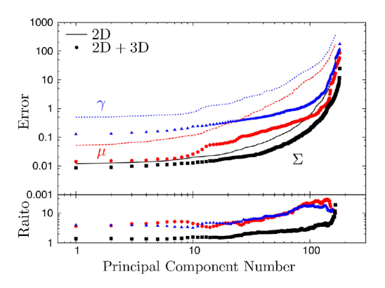
Figure 1: The upper panels show the uncertainties in the amplitudes of the principal components (eigenmodes) of $\mu$ (red circles), $\gamma$ (blue triangles) and $\Sigma$ (black squares) from 2D+3D information. The number of principal components is ordered from small to large $\sigma$. For comparison, the lines shows the corresponding errors obtained from the 2D information only. The lower panel shows the ratio of errors for the eigenmodes with the same order number, which indicates the extent to which the eigenmodes are better constrained by adding the 3D information. Cosmological parameters and the galaxy bias parameters are marginalized over.

In this section we show the results of the principal component analysis of $\mu$, $\gamma$ and $\Sigma$ from 2D measurements (CMB, WL and GC auto- and cross-spectra) combined with 3D measurements of the galaxy redshift-space power spectra. We particularly focus on how the 3D information improves the constraints on the eigenmodes of $\mu$, $\gamma$ and $\Sigma$.

First we investigate the degeneracy of MG parameters with $6$ cosmological parameters and the bias parameters. Table 2 lists the forecasted uncertainties in the cosmological parameters from the combinations of the various observations. The cosmological parameters are constrained mainly by CMB data, while large-scale structure measurements significantly improve the accuracy of $\Omega_{c}h^{2}$ and $h$ because they are sensitive to $\Omega_{c}$. When adding $\mu(k,z)$ and $\gamma(k,z)$ as free parameters, the marginalized constraints on cosmological parameters weaken by up to 50% mainly due to the strong degeneracy between the amplitude $A_{s}$ and the MG parameters: the change of the initial fluctuation amplitude can be compensated by the overall change of $\mu$. We also find that the error on bias parameters in tomographic and spectroscopic bins increases only by about 10% after adding MG parameters. The degeneracy of the galaxy bias with MG parameters is small because we use the linear bias that does not depend on scale and almost all the well-constrained eigenmodes in figure 2 are oscillating along $k$-axis. Degeneracies between the cosmological parameters and different sets of MG parameters have been studied in detail in [59].

The upper panel of figure 1 shows the forecasted errors on amplitudes of principal components (eigenmodes) in the ascending order of $\sigma$, i.e. the eigenmodes are ordered from best constrained to worst. The lines represent the errors on eigenmodes of $\mu$, $\gamma$ and $\Sigma$ from 2D only, while symbols represent the corresponding errors from a combination of 2D with 3D. In all cases, the covariance matrix is estimated by taking the inverse of a $(2mn+6+N_{b})\times(2mn+6+N_{b})$ Fisher matrix, but the eigenmodes and eigenvalues are estimated by separately diagonalizing the $mn\times mn$ covariance submatrices associated with $\mu$ and $\gamma$. The covariance matrix of $\Sigma$ is calculated by using eq. (2.15). The lower panel of figure 1 represents the ratio of the errors of eigenmodes with the same principal component number between 2D and 2D+3D. We find that adding 3D reduces the errors of $\mu$ and $\gamma$ by a factor between $3$ and $10$.

Note that the plots in figure 1 just compare the eigenvalues with and without 3D information. They do not provide any information about the amplitude of the corresponding modes in modified gravity theories. For example, for some of these theories, departure from the fiducial value of $\Sigma$ (and hence the amplitude of the oscillating modes) is small. The Fisher matrices for parameters in specific MG models can be calculated by projecting errors on the parameters from principal components without regenerating the Fisher matrix from scratch [39, 40]. This projection was done for a one-parameter model of $\mu(k,a)$ and $\gamma(k,a)$ which gives a good approximations for $f(R)$ theories in quasi-static limits in Ref. [40] using only 2D information. We leave detailed studies of the effects of adding 3D information on constraining parameters in specific MG models for future work.

Note that we used different redshift ranges for 2D only and 2D+3D measurements: $0.8\leq z\leq 3.0$ for 2D only and $0.4\leq z\leq 2.8$ for 2D+3D. Here we consider the spectroscopic samples where galaxies populate at the redshift from 0.4 to 2 and then MG parameters are strongly degenerate outside this redshift range. Accordingly, the number of $z$-bins changes from $n=11$ (2D) to $n=12$ (2D+3D) with the binning width fixed to be 0.2 in redshift. Even though the maximum redshift for 2D+3D is smaller than that for 2D only, the result is insensitive to the maximum redshift because the number of observed galaxies at high redshift is small. A quantitative study on the effect of varying $\mu$ and $\gamma$ at high-$z$ is left for future work. A significant result of adding the 3D information is that the number of eigenmodes with $\sigma<1$ increases from $40$ to $123$ for $\mu$, from $11$ to $81$ for $\gamma$ and from $110$ to $140$ for $\Sigma$ after adding the 3D information. This improvement comes from the additional information in the radial modes provided by the 3D data. For $\Sigma$, eigenmodes are primarily constrained from WL observables and thus the improvement from adding the 3D information is relatively small.

Figure 2 shows the first 16 principal component modes (eigenmodes) with small uncertainties for $\mu$, $\gamma$ and $\Sigma$, from top to bottom, in 2D (left) and 2D+3D (right). Each mini-panel describes ${\bf w}_{i}$ (eq. (2.14)) in the $(k,z)$ space (colours represent the amplitude). As shown in [40], if only the 2D measurements are used, the best constrained eigenmodes show oscillations in $k$, while new $z$-oscillation modes appear after each dozen or so $k$-oscillation modes. This indicates that the scale dependence of $\mu$ and $\gamma$ is much better constrained than the $z$-dependence. This is because the departure of $\mu$ from unity at a certain $z_{i}$ affects the clustering at all lower $z$ and thus the degeneracy along $z$-axis becomes strong. Also, the WL kernel for a given angular moment $\ell$ receives contributions from $k$ and $z$ over a relatively wide range, and directly probes $\Sigma$ rather than $\mu$ and $\gamma$ individually. This results in an additional loss of sensitivity to the dependence of $\mu$ on $z$. On the other hand, when the 3D measurements are added, each eigenmode becomes sensitive to $\mu$ at a certain $k$ because the departure of $\mu$ from unity at a certain scale $k$ affects the 3D galaxy power spectrum only at the corresponding scale in the linear approximation. This is the reason why the eigenmodes of $\mu$ after adding the 3D measurements have peaks around a certain $k$. Some of the eigenmodes of $\gamma$ (e.g. the $7$-th, $9$-th and $12$-th) are also sensitive to specific scales, but the other eigenmodes still show oscillations in $k$ because $\gamma$ is constrained by both the angular power spectra and the galaxy power spectra. On the other hand, $\Sigma$ is mainly determined by the 2D measurements thus their eigenmodes do not change much even if we add the 3D information.

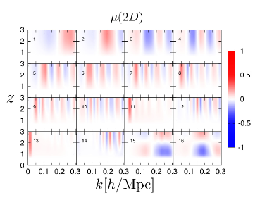
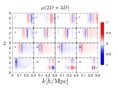
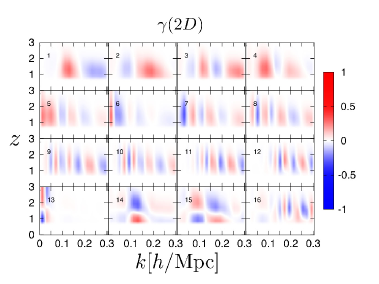
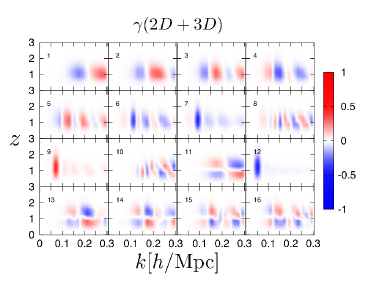
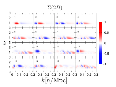
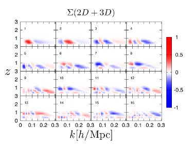
Figure 2: Eigenmodes of $\mu$, $\gamma$, and $\Sigma$ from top to bottom. The left panels show the eigenmodes calculated from the 2D information (WL$\times$GC$\times$CMB) and the right panels are those from the 2D+3D information.

5 Degeneracies between $\mu$ and $\gamma$

In order to understand the cause of the degeneracy between $\mu$ and $\gamma$, and how the 3D information resolves it, we consider the simplest case where the MG parameters consist of just 2 parameters $\mu$ and $\gamma$ at some specific $k$ and $z$ and neglect the correlation with other $k$ and $z$. We also ignore the degeneracy with other parameters, such as $\Omega_{M}$ and the bias, here for simplicity.

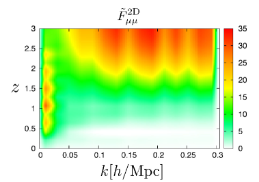
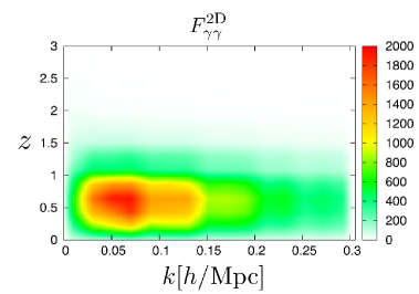
Figure 3: Left and right panels show the values of $\tilde{F}_{\mu\mu}$ and $F_{\gamma\gamma}$ representing the inverse of the variance of $\mu$ and $\Sigma$ (see eqs. (5.14) and (5.15)), respectively, at different $k$ and $z$.

First we consider the 2D measurements only. From the relation between the lensing potential and the matter perturbation, eq. (2.10),

$$C_{\ell}^{\rm WL}\propto[\mu(1+\gamma)/2]^{2},$$ (5.1)

and the derivatives of the angular power spectra with respect to $\mu$ and $\gamma$ are given by

$$\frac{\partial C^{\rm WL}_{\ell}}{\partial\mu} \propto\mu(1+\gamma)^{2}/2,$$ (5.2)

$$\frac{\partial C^{\rm WL}_{\ell}}{\partial\gamma} \propto\mu^{2}(1+\gamma)/2.$$ (5.3)

Therefore, the response of $\mu$ and $\gamma$ to the angular power spectra of WL has the following relation:

$$\frac{\partial C^{\rm WL}_{\ell}}{\partial\mu}=\frac{(1+\gamma)}{\mu}\frac{\partial C^{\rm WL}_{\ell}}{\partial\gamma}=2\frac{\partial C^{\rm WL}_{\ell}}{\partial\gamma},$$ (5.4)

where we used the fiducial values of $\mu$ and $\gamma$, $\mu=\gamma=1$. Thus the Fisher information given by WL has the relation of $F^{\rm WL}_{\mu\mu}=4F^{\rm WL}_{\gamma\gamma}$, and, thereby, the parameters of $\mu$ and $\gamma$ are completely degenerate with each other. Note that the lensing potential has additional $\mu$-dependence through the growth of the density perturbation $\delta$ but this additional $\mu$-dependence is weak and also this does not change the fact that $\mu$ and $\gamma$ are completely degenerate in WL measurements. We found that the dominant contribution of the 2D measurements comes from WL auto-correlations and cross-correlations between WL and GC through magnification bias effects and this is the origin of the degeneracy between $\mu$ and $\gamma$ when only the 2D measurements are used.

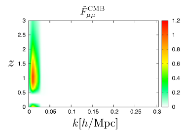
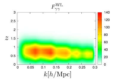
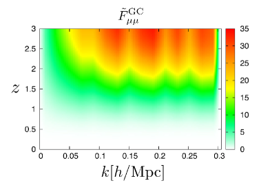
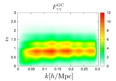
Figure 4: The contributions of CMB, WL and GC (in the order from top to bottom) auto correlations to $\tilde{F}_{\mu\mu}^{\rm 2D}$ (left panels) and $F_{\gamma\gamma}^{\rm 2D}$ (right panels).

Assuming that $\mu$ and $\gamma$ are maximally correlated, i.e., $F^{\rm 2D}_{\mu\gamma}=\sqrt{F^{\rm 2D}_{\mu\mu}F^{\rm 2D}_{\gamma\gamma}}\sim 2F^{\rm 2D}_{\gamma\gamma}$, we find that the total Fisher matrix from 2D measurements can be approximated as

$${\bf F}=\left(\begin{array}[]{cc}F^{\rm 2D}_{\gamma\gamma}&F^{\rm 2D}_{\gamma\mu}\\ F^{\rm 2D}_{\mu\gamma}&F^{\rm 2D}_{\mu\mu}\end{array}\right)=\left(\begin{array}[]{cc}F^{\rm 2D}_{\gamma\gamma}&2F^{\rm 2D}_{\gamma\gamma}\\ 2F^{\rm 2D}_{\gamma\gamma}&4F^{\rm 2D}_{\gamma\gamma}+\tilde{F}^{\rm 2D}_{\mu\mu}\end{array}\right),$$ (5.9)

where $\tilde{F}^{\rm 2D}_{\mu\mu}\equiv F^{\rm 2D}_{\mu\mu}-4F^{\rm 2D}_{\gamma\gamma}$. As the value of $\tilde{F}^{\rm 2D}_{\mu\mu}$ is smaller, the degeneracy between $\mu$ and $\gamma$ is larger. The determinant of the Fisher matrix becomes $\det{{\bf F}}=F^{\rm 2D}_{\gamma\gamma}\tilde{F}^{\rm 2D}_{\mu\mu}$, and the covariance matrix is given by

$${\bf C}={\bf F}^{-1}=\left(\begin{array}[]{cc}4(\tilde{F}_{\mu\mu}^{\rm 2D})^{-1}+(F_{\gamma\gamma}^{\rm 2D})^{-1}&-2(\tilde{F}_{\mu\mu}^{\rm 2D})^{-1}\\ -2(\tilde{F}_{\mu\mu}^{\rm 2D})^{-1}&(\tilde{F}_{\mu\mu}^{\rm 2D})^{-1}\end{array}\right).$$ (5.12)

The variances of $\mu$ and $\gamma$ are respectively given in terms of $\tilde{F}_{\mu\mu}^{\rm 2D}$ and $F_{\gamma\gamma}^{\rm 2D}$ as

$$C_{\gamma\gamma} =4(\tilde{F}_{\mu\mu}^{\rm 2D})^{-1}+(F_{\gamma\gamma}^{\rm 2D})^{-1},$$ (5.13)

$$C_{\mu\mu} =(\tilde{F}_{\mu\mu}^{\rm 2D})^{-1},$$ (5.14)

and, from eq. (2.15), the variance of $\Sigma$ is given by

$$C_{\Sigma\Sigma}=(4F_{\gamma\gamma}^{\rm 2D})^{-1}.$$ (5.15)

From eqs. (5.14) and (5.15), $\tilde{F}_{\mu\mu}^{\rm 2D}$ and $F_{\gamma\gamma}^{\rm 2D}$ represent the inverse of covariance of $\mu$ and $\Sigma$ respectively. From eq. (5.13), we find that both the values of $\tilde{F}_{\mu\mu}^{\rm 2D}$ and $F_{\gamma\gamma}^{\rm 2D}$ have to be larger than unity to constrain $\gamma$ well.

However, it is difficult to obtain large $\tilde{F}_{\mu\mu}^{\rm 2D}$ and $F_{\gamma\gamma}^{\rm 2D}$ simultaneously at any redshifts from 2D measurements only. Figure 3 shows the values of $\tilde{F}_{\mu\mu}^{\rm 2D}$ and $F_{\gamma\gamma}^{\rm 2D}$ at each $k$ and $z$. The value of $\tilde{F}_{\mu\mu}^{\rm 2D}$ is larger at higher redshifts because a change of $\mu$ at high $z$ affects the growth of structure at all lower $z$. On the other hand, $F_{\gamma\gamma}^{\rm 2D}$ has large values at low redshifts ($z\lower 2.15277pt\hbox{$\;\buildrel<\over{\sim}\;$}1$) because WL is only sensitive to the change of $\gamma$ between the source galaxies and the observer. Such differences in redshift ranges where $\mu$ and $\gamma$ can be sensitively probed make it difficult to reduce the degeneracy between $\mu$ and $\gamma$ at all redshifts. Furthermore, the constraints on $\mu$ from 2D measurements are much weaker ($\tilde{F}_{\mu\mu}^{\rm 2D}$ is smaller) compared to the constraints on $\Sigma$, and thus the constraints on $\mu$ and $\gamma$ become weak.

Figure 4 shows the contribution of each 2D measurement, i.e., CMB, WL, and GC to $\tilde{F}_{\mu\mu}^{\rm 2D}$ (left) and $F_{\gamma\gamma}^{\rm 2D}$ (right). Cross-correlations among different measurements are not included in this figure. We can see that the main contribution to $\tilde{F}_{\mu\mu}^{\rm 2D}$ comes from GC, while the main contribution to $F_{\gamma\gamma}^{\rm 2D}$ comes from WL, which is as expected. The ISW effect in CMB affects $F_{\gamma\gamma}^{\rm CMB}$ at small $k$ and low $z$. From figure 4, we find the contribution of ISW is smaller than other contributions, because the ISW effect appears on large scales where the number of modes, given by $2\ell+1$, is smaller. Moreover we can assume that $\tilde{F}^{\rm CMB}_{\mu\mu}$ is zero. Thus, CMB is not directly constraining the modified gravity parameters. However, it helps to reduce the degeneracies between cosmological parameters and the MG parameters, thus tightening the constraints on MG parameters after marginalizing over cosmological parameters [59]. The contribution of WL to $\tilde{F}_{\mu\mu}^{\rm WL}$ is non-zero because the number distribution of source galaxies is changed by $\mu$ at high-$k$. $F^{\rm GC}_{\gamma\gamma}$ in figure 4 comes from the magnification bias effects. The reason that $F^{\rm 2D}_{\gamma\gamma}\gg F^{\rm CMB}_{\gamma\gamma}+F^{\rm WL}_{\gamma\gamma}+F^{\rm GC}_{\gamma\gamma}$ is that the cross correlations, especially ${\rm WL}\times{\rm GC}$ (galaxy-galaxy lensing) are powerful tools for deriving information from weak lensing.

Figure 5: Fisher matrix of $\mu$ from the 3D galaxy power spectra $F_{\mu\mu}^{3D}$ (eq. (3.18)).

Next we see how the situation changes by adding in the 3D information. We denote the Fisher information of $\mu$ and $\gamma$ from 3D as $F_{\mu\mu}^{\rm 3D}$ and $F_{\gamma\gamma}^{\rm 3D}$, respectively, and we assume $F_{\gamma\gamma}^{\rm 3D}=0$. The determinant of the Fisher matrix and the variances of $\mu$ and $\gamma$ are given by

$$\det{\bf F} =(\tilde{F}_{\mu\mu}^{\rm 2D}+F^{\rm 3D}_{\mu\mu})F_{\gamma\gamma}^{\rm 2D},$$ (5.16)

$$C_{\gamma\gamma} =4(\tilde{F}_{\mu\mu}^{\rm 2D}+F^{\rm 3D}_{\mu\mu})^{-1}+(F_{\gamma\gamma}^{\rm 2D})^{-1},$$ (5.17)

$$C_{\mu\mu} =(\tilde{F}_{\mu\mu}^{\rm 2D}+F^{\rm 3D}_{\mu\mu})^{-1}.$$ (5.18)

One can see that $F^{3D}_{\mu\mu}$ plays the same role as $\tilde{F}^{\rm 2D}_{\mu\mu}$ in reducing the degeneracy between $\mu$ and $\gamma$ because the correlation coefficient becomes

$$\frac{C_{\gamma\mu}}{\sqrt{C_{\gamma\gamma}C_{\mu\mu}}} =-\left(1+\frac{\tilde{F}_{\mu\mu}^{\rm 2D}}{4F_{\gamma\gamma}^{\rm 2D}}\right)^{-1/2}\ {\rm(2D\ only)},$$

$$=-\left(1+\frac{\tilde{F}_{\mu\mu}^{\rm 2D}+F^{\rm 3D}_{\mu\mu}}{4F_{\gamma\gamma}^{\rm 2D}}\right)^{-1/2}\ ({\rm 2D+3D}).$$ (5.19)

Figure 6: The correlation coefficient eq. (5.19) in $(k,z)$ space by using only 2D only (left) and 2D+3D (right)

Figure 5 shows that $F_{\mu\mu}^{\rm 3D}$ is much larger than $\tilde{F}^{\rm 2D}_{\mu\mu}$ in the left panel of figure 3. Therefore, the 3D information of the galaxy power spectra significantly improves the constraints on the parameters of $\mu$ and $\gamma$ and reduce the degeneracy between $\mu$ and $\gamma$. Figure 6 shows the correlation coefficient between $\mu$ and $\gamma$ with and without the 3D information. The correlation coefficient is almost unity at $z<2$, meaning that $\mu$ and $\gamma$ have perfect degeneracy. However, the parameter space for the maximal degeneracy gets narrowed down to $z\lesssim 1.5$ when the 3D information is added in. The reason for this degeneracy at $z\lesssim 1.5$ is that the signal of the weak lensing dominates here. However, we find that the degeneracy between $\mu$ and $\gamma$ becomes weaker by adding the 3D information. Quantitatively, it results in a factor between $3$ and $10$ reduction of the errors over the redshift range that galaxy spectroscopic survey covers.

Note that, in principle the 3D information is not independent of GC, thus the correlation needs to be taken into account when combining them. But we ignore the correlation here since $F^{\rm 3D}_{\mu\mu}\gg\tilde{F}_{\mu\mu}^{\rm 2D}$ as seen from figure 5 and the left panel of figure 3.

6 Summary and Conclusions

We performed a principal component analysis (PCA) to forecast the ability of future observations to measure departures from GR in Poisson, anisotropy and lensing potential equations parametrized by $\mu(k,z)$, $\gamma(k,z)$ and $\Sigma(k,z)$, respectively, in a model-independent way. We found that the galaxy power spectra in the redshift-space is a powerful tool for constraining $\mu$ and $\gamma$. Combining galaxy redshift surveys like BOSS and Euclid surveys with weak lensing tomography decreases the error on principal component modes by a factor between $3$ and $10$, and increases the number of informative modes approximately by a factor of $3$ for $\mu$ and by $7$ for $\gamma$. Such a gain in constraining MG parameters mainly comes from the fact that redshift-space distortion measurements from galaxy redshift surveys are a powerful tool to constrain $\mu$ and reduce the degeneracy between $\mu$ and $\gamma$, while lensing only constrains their combinations. Further, as shown in table 2, we find that the constraints on parameters of the modified gravity remain strong even if we take into account the uncertainty of cosmological parameters, because CMB measurements strongly constrain the cosmological parameters.

Our analysis neglects various systematic errors. For lensing, these include possible shifts of the centroids and the dispersion of photo $z$-bins photometric redshift error, and the shape measurement error (see appendix in [40] for details). We also adopt a linear Kaiser formula to describe the redshift-space galaxy power spectra. More accurate formulae using $P_{\delta\theta}$ and velocity auto spectrum $P_{\theta\theta}$ are proposed by [60, 61, 62]. We neglect various non-linear effects on the galaxy clustering in redshift space. Nonlinearity in galaxy biasing should be important at small scales and increases the uncertainty in measuring $\mu$. Nonlinear redshift distortion effect, i.e., Finger-of-God effects, generates systematic uncertainties in the measurements of RSD [63]. Cross-correlation measurements with WL decreases the uncertainty of FoG effect by measuring the off-centering of satellite galaxies [64]. Such improvements in the theoretical modeling are left for future work.

Appendix A Combined modes

In the main text, we showed the eigenmodes obtained by diagonalizing independently the covariance matrix for $\mu$, $\gamma$ or $\Sigma$. We can instead obtain the eigenmodes in the whole $(\mu,\gamma)$ or $(\mu,\Sigma)$ parameter space. In other words, we can diagonalize the $2mn\times 2mn$ covariance matrix which contains $\mu$, ($\gamma$ or $\Sigma$) and cross-covariance of the two parameters. We call the eigenmodes obtained in this way the $(\mu,\gamma)$ or $(\mu,\Sigma)$ combined modes. We also call the part of the combined eigenmode associated with $\mu$ ($\gamma$ or $\Sigma$) the $\mu$ ($\gamma$ or $\Sigma$) surface.

Adding the information of the galaxy power spectra in the redshift-space increases the numbers of eigenmodes of the $(\mu,\gamma)$ and $(\mu,\Sigma)$ combined modes with $\sigma<1$ from 141 to 237 and from 152 to 265, respectively. In the following, we show the result after adding the 3D information. Figure 7 shows the error of the $(\mu,\gamma)$ or $(\mu,\Sigma)$ combined modes, and figure 8 shows the combined modes.

Figure 7: The error of the eigenmodes calculated from 2D and 3D. The triangle dots with the lines are the same as figure 1. The magenta square dots and the cyan circle dots are the error on the $(\mu,\gamma)$ and $(\mu,\Sigma)$ combined modes respectively. The mini-figure show the results enlarged where the principle component number is smaller.

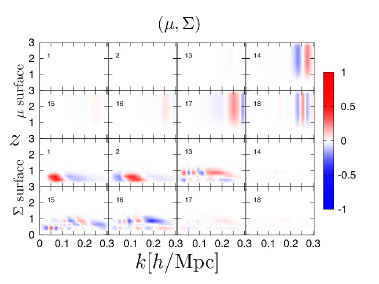
Figure 8: The parameter-surfaces of the combined modes. The left panel show the eigenmodes of the $(\mu,\gamma)$ combined modes and the right panel show the eigenmodes of the $(\mu,\Sigma)$ combined mode.

From figure 8, we find that the $\mu$-surfaces and the $\Sigma$-surfaces of the $(\mu,\Sigma)$ combined modes are almost independent. In other words, when one of the surfaces has nodes, i.e. the regions that are constrained better, the other surface is hardly constrained. The reason is that $\mu$ and $\Sigma$ are individually constrained from the galaxy distribution and the weak lensing respectively as we expect from eqs. (5.15) and (5.18). Moreover, the best-constrained eigenmode is the eigenmode constraining $\Sigma$, because $\max{[4F^{\rm 2D}_{\gamma\gamma}(k.z)]}>\max{[\tilde{F}_{\mu\mu}^{\rm 2D}(k,z)+F^{\rm 3D}_{\mu\mu}(k,z)]}$. The eigenmode that has a distinct node on the $\mu$-surface appears in the 14th $(\mu,\Sigma)$ combined eigenmode because from figure 7 the error on the best-constrained eigenmode of $\mu$ is larger than the error on the 13th eigenmode of $\Sigma$ and smaller than the error on the 14th eigenmodes of $\Sigma$.

On the other hand, the $\mu$-surfaces and $\gamma$-surfaces of the $(\mu,\gamma)$ combined modes have the same shapes and they have similar shapes to the eigenmodes of $\Sigma$ up to the 16th eigenmodes. This is because $\Sigma$ is expressed as a combination of $\mu$ and $\gamma$, and the constraints from the weak lensing is the strongest. The error on the best-constrained $(\mu,\gamma)$ combined mode is smaller than that of the $(\mu,\Sigma)$ combined modes because there is a degree of freedom in dividing the deviation of weak lensing measurements from $\Lambda$CDM into $\mu$ and $\gamma$, and $\mu$ at low-z, where we gain the most information from weak lensing, is constrained only weakly by the galaxy distribution.

Moreover the shape of $(\mu,\gamma)$ combined eigenmodes is a mixture of the $\mu$ and $\Sigma$ eigenmodes. For example, the elongated feature in $z$-direction at $k=0.2-0.3$ clearly seen in the 16 or 17th mode comes from the first eigenmode of $\mu$ (see the top-right panel in figure 2). This can be understood from the minipanel of figure 7 because the error of the best-constrained mode of $\mu$ is nearly equal to the error of the 17th $(\mu,\gamma)$ combined mode.

References

- [1] A. G. Riess, A. V. Filippenko, P. Challis, A. Clocchiatti, A. Diercks, P. M. Garnavich, R. L. Gilliland, C. J. Hogan, S. Jha, R. P. Kirshner, B. Leibundgut, M. M. Phillips, D. Reiss, B. P. Schmidt, R. A. Schommer, R. C. Smith, J. Spyromilio, C. Stubbs, N. B. Suntzeff, and J. Tonry, Observational Evidence from Supernovae for an Accelerating Universe and a Cosmological Constant, AJ 116 (Sept., 1998) 1009–1038, [astro-ph/9805201].
- [2] S. Perlmutter, G. Aldering, G. Goldhaber, R. A. Knop, P. Nugent, P. G. Castro, S. Deustua, S. Fabbro, A. Goobar, D. E. Groom, I. M. Hook, A. G. Kim, M. Y. Kim, J. C. Lee, N. J. Nunes, R. Pain, C. R. Pennypacker, R. Quimby, C. Lidman, R. S. Ellis, M. Irwin, R. G. McMahon, P. Ruiz-Lapuente, N. Walton, B. Schaefer, B. J. Boyle, A. V. Filippenko, T. Matheson, A. S. Fruchter, N. Panagia, H. J. M. Newberg, W. J. Couch, and Supernova Cosmology Project, Measurements of Omega and Lambda from 42 High-Redshift Supernovae, ApJ 517 (June, 1999) 565–586, [astro-ph/9812133].
- [3] The Planck Collaboration, The Scientific Programme of Planck, ArXiv Astrophysics e-prints (Apr., 2006) [astro-ph/0604069].
- [4] A. G. Sánchez, C. G. Scóccola, A. J. Ross, W. Percival, M. Manera, F. Montesano, X. Mazzalay, A. J. Cuesta, D. J. Eisenstein, E. Kazin, C. K. McBride, K. Mehta, A. D. Montero-Dorta, N. Padmanabhan, F. Prada, J. A. Rubiño-Martín, R. Tojeiro, X. Xu, M. V. Magaña, E. Aubourg, N. A. Bahcall, S. Bailey, D. Bizyaev, A. S. Bolton, H. Brewington, J. Brinkmann, J. R. Brownstein, J. R. Gott, J. C. Hamilton, S. Ho, K. Honscheid, A. Labatie, E. Malanushenko, V. Malanushenko, C. Maraston, D. Muna, R. C. Nichol, D. Oravetz, K. Pan, N. P. Ross, N. A. Roe, B. A. Reid, D. J. Schlegel, A. Shelden, D. P. Schneider, A. Simmons, R. Skibba, S. Snedden, D. Thomas, J. Tinker, D. A. Wake, B. A. Weaver, D. H. Weinberg, M. White, I. Zehavi, and G. Zhao, The clustering of galaxies in the SDSS-III Baryon Oscillation Spectroscopic Survey: cosmological implications of the large-scale two-point correlation function, Mon. Not. Roy. Astron. Soc. 425 (Sept., 2012) 415–437, [arXiv:1203.6616].
- [5] C. Wetterich, Cosmology and the fate of dilatation symmetry, Nuclear Physics B 302 (June, 1988) 668–696.
- [6] T. Chiba, T. Okabe, and M. Yamaguchi, Kinetically driven quintessence, Phys. Rev. D 62 (July, 2000) 023511, [astro-ph/9912463].
- [7] J. D. Bekenstein, Relativistic gravitation theory for the modified Newtonian dynamics paradigm, Phys. Rev. D 70 (Oct., 2004) 083509, [astro-ph/0403694].
- [8] G. Dvali, G. Gabadadze, and M. Porrati, 4D gravity on a brane in 5D Minkowski space, Physics Letters B 485 (July, 2000) 208–214, [hep-th/0005016].
- [9] M. Milgrom, A modification of the Newtonian dynamics - Implications for galaxies, ApJ 270 (July, 1983) 371–389.
- [10] C. Eling, T. Jacobson, and D. Mattingly, Einstein-Aether Theory, ArXiv General Relativity and Quantum Cosmology e-prints (Sept., 2004) [gr-qc/0410001].
- [11] S. Capozziello, S. Carloni, and A. Troisi, Quintessence without scalar fields, ArXiv Astrophysics e-prints (Mar., 2003) [astro-ph/0303041].
- [12] S. M. Carroll, V. Duvvuri, M. Trodden, and M. S. Turner, Is cosmic speed-up due to new gravitational physics?, Phys. Rev. D 70 (Aug., 2004) 043528, [astro-ph/0306438].
- [13] A. Nicolis, R. Rattazzi, and E. Trincherini, Galileon as a local modification of gravity, Phys. Rev. D 79 (Mar., 2009) 064036, [arXiv:0811.2197].
- [14] T. Clifton, P. G. Ferreira, A. Padilla, and C. Skordis, Modified gravity and cosmology, Phys. Rep. 513 (Mar., 2012) 1–189, [arXiv:1106.2476].
- [15] H. Oyaizu, M. Lima, and W. Hu, Nonlinear evolution of f(R) cosmologies. II. Power spectrum, Phys. Rev. D 78 (Dec., 2008) 123524, [arXiv:0807.2462].
- [16] G.-B. Zhao, B. Li, and K. Koyama, N-body simulations for f(R) gravity using a self-adaptive particle-mesh code, Phys. Rev. D 83 (Feb., 2011) 044007, [arXiv:1011.1257].
- [17] B. Li, G.-B. Zhao, R. Teyssier, and K. Koyama, ECOSMOG: an Efficient COde for Simulating MOdified Gravity, JCAP 1 (Jan., 2012) 51, [arXiv:1110.1379].
- [18] E. Puchwein, M. Baldi, and V. Springel, Modified Gravity-GADGET: A new code for cosmological hydrodynamical simulations of modified gravity models, ArXiv e-prints (May, 2013) [arXiv:1305.2418].
- [19] “http://www.darkenergysurvey.org/.”
- [20] “http://www.sdss3.org/surveys/boss.php.”
- [21] “http://www.lsst.org/.”
- [22] “http://sumire.ipmu.jp/en/.”
- [23] D. J. Schlegel, C. Bebek, H. Heetderks, S. Ho, M. Lampton, M. Levi, N. Mostek, N. Padmanabhan, S. Perlmutter, N. Roe, M. Sholl, G. Smoot, M. White, A. Dey, T. Abraham, B. Jannuzi, D. Joyce, M. Liang, M. Merrill, K. Olsen, and S. Salim, BigBOSS: The Ground-Based Stage IV Dark Energy Experiment, ArXiv e-prints (Apr., 2009) [arXiv:0904.0468].
- [24] “http://bigboss.lbl.gov/.”
- [25] “http://hetdex.org/.”
- [26] “http://www.euclid-ec.org.”
- [27] G.-B. Zhao, L. Pogosian, A. Silvestri, and J. Zylberberg, Searching for modified growth patterns with tomographic surveys, Phys. Rev. D 79 (Apr., 2009) 083513, [arXiv:0809.3791].
- [28] L. Pogosian, A. Silvestri, K. Koyama, and G.-B. Zhao, How to optimally parametrize deviations from general relativity in the evolution of cosmological perturbations, Phys. Rev. D 81 (May, 2010) 104023, [arXiv:1002.2382].
- [29] P. Zhang, M. Liguori, R. Bean, and S. Dodelson, Probing Gravity at Cosmological Scales by Measurements which Test the Relationship between Gravitational Lensing and Matter Overdensity, Physical Review Letters 99 (Oct., 2007) 141302, [arXiv:0704.1932].
- [30] L. Amendola, M. Kunz, and D. Sapone, Measuring the dark side (with weak lensing), JCAP 4 (Apr., 2008) 13, [arXiv:0704.2421].
- [31] W. Hu and I. Sawicki, Parametrized post-Friedmann framework for modified gravity, Phys. Rev. D 76 (Nov., 2007) 104043, [arXiv:0708.1190].
- [32] T. Baker, P. G. Ferreira, C. Skordis, and J. Zuntz, Towards a fully consistent parametrization of modified gravity, Phys. Rev. D 84 (Dec., 2011) 124018, [arXiv:1107.0491].
- [33] J. Zuntz, T. Baker, P. G. Ferreira, and C. Skordis, Ambiguous tests of general relativity on cosmological scales, JCAP 6 (June, 2012) 32, [arXiv:1110.3830].
- [34] T. Baker, P. G. Ferreira, and C. Skordis, The parameterized post-Friedmann framework for theories of modified gravity: Concepts, formalism, and examples, Phys. Rev. D 87 (Jan., 2013) 024015, [arXiv:1209.2117].
- [35] R. A. Battye and J. A. Pearson, Massive gravity, the elasticity of space-time and perturbations in the dark sector, ArXiv e-prints (Jan., 2013) [arXiv:1301.5042].
- [36] G.-B. Zhao, T. Giannantonio, L. Pogosian, A. Silvestri, D. J. Bacon, K. Koyama, R. C. Nichol, and Y.-S. Song, Probing modifications of general relativity using current cosmological observations, Phys. Rev. D 81 (May, 2010) 103510, [arXiv:1003.0001].
- [37] L. Samushia, B. A. Reid, M. White, W. J. Percival, A. J. Cuesta, L. Lombriser, M. Manera, R. C. Nichol, D. P. Schneider, D. Bizyaev, H. Brewington, E. Malanushenko, V. Malanushenko, D. Oravetz, K. Pan, A. Simmons, A. Shelden, S. Snedden, J. L. Tinker, B. A. Weaver, D. G. York, and G.-B. Zhao, The clustering of galaxies in the SDSS-III DR9 Baryon Oscillation Spectroscopic Survey: testing deviations from and general relativity using anisotropic clustering of galaxies, Mon. Not. Roy. Astron. Soc. 429 (Feb., 2013) 1514–1528, [arXiv:1206.5309].
- [38] F. Simpson, C. Heymans, D. Parkinson, C. Blake, M. Kilbinger, J. Benjamin, T. Erben, H. Hildebrandt, H. Hoekstra, T. D. Kitching, Y. Mellier, L. Miller, L. Van Waerbeke, J. Coupon, L. Fu, J. Harnois-Déraps, M. J. Hudson, K. Kuijken, B. Rowe, T. Schrabback, E. Semboloni, S. Vafaei, and M. Velander, CFHTLenS: testing the laws of gravity with tomographic weak lensing and redshift-space distortions, Mon. Not. Roy. Astron. Soc. 429 (Mar., 2013) 2249–2263, [arXiv:1212.3339].
- [39] G.-B. Zhao, L. Pogosian, A. Silvestri, and J. Zylberberg, Cosmological Tests of General Relativity with Future Tomographic Surveys, Physical Review Letters 103 (Dec., 2009) 241301, [arXiv:0905.1326].
- [40] A. Hojjati, G.-B. Zhao, L. Pogosian, A. Silvestri, R. Crittenden, and K. Koyama, Cosmological tests of general relativity: A principal component analysis, Phys. Rev. D 85 (Feb., 2012) 043508, [arXiv:1111.3960].
- [41] A. Hall, C. Bonvin, and A. Challinor, Testing general relativity with 21-cm intensity mapping, Phys. Rev. D 87 (Mar., 2013) 064026, [arXiv:1212.0728].
- [42] N. Kaiser, Clustering in real space and in redshift space, Mon. Not. Roy. Astron. Soc. 227 (July, 1987) 1–21.
- [43] J. Guzik, B. Jain, and M. Takada, Tests of gravity from imaging and spectroscopic surveys, Phys. Rev. D 81 (Jan., 2010) 023503, [arXiv:0906.2221].
- [44] Y.-S. Song, G.-B. Zhao, D. Bacon, K. Koyama, R. C. Nichol, and L. Pogosian, Complementarity of weak lensing and peculiar velocity measurements in testing general relativity, Phys. Rev. D 84 (Oct., 2011) 083523, [arXiv:1011.2106].
- [45] Planck Collaboration, P. A. R. Ade, N. Aghanim, C. Armitage-Caplan, M. Arnaud, M. Ashdown, F. Atrio-Barandela, J. Aumont, C. Baccigalupi, A. J. Banday, and et al., Planck 2013 results. XVI. Cosmological parameters, ArXiv e-prints (Mar., 2013) [arXiv:1303.5076].
- [46] L. Amendola, S. Appleby, D. Bacon, T. Baker, M. Baldi, N. Bartolo, A. Blanchard, C. Bonvin, S. Borgani, E. Branchini, C. Burrage, S. Camera, C. Carbone, L. Casarini, M. Cropper, C. deRham, C. di Porto, A. Ealet, P. G. Ferreira, F. Finelli, J. Garcia-Bellido, T. Giannantonio, L. Guzzo, A. Heavens, L. Heisenberg, C. Heymans, H. Hoekstra, L. Hollenstein, R. Holmes, O. Horst, K. Jahnke, T. D. Kitching, T. Koivisto, M. Kunz, G. La Vacca, M. March, E. Majerotto, K. Markovic, D. Marsh, F. Marulli, R. Massey, Y. Mellier, D. F. Mota, N. Nunes, W. Percival, V. Pettorino, C. Porciani, C. Quercellini, J. Read, M. Rinaldi, D. Sapone, R. Scaramella, C. Skordis, F. Simpson, A. Taylor, S. Thomas, R. Trotta, L. Verde, F. Vernizzi, A. Vollmer, Y. Wang, J. Weller, and T. Zlosnik, Cosmology and fundamental physics with the Euclid satellite, ArXiv e-prints (June, 2012) [arXiv:1206.1225].
- [47] E. L. Turner, J. P. Ostriker, and J. R. Gott, III, The statistics of gravitational lenses - The distributions of image angular separations and lens redshifts, ApJ 284 (Sept., 1984) 1–22.
- [48] J. Verner Villumsen, Clustering of Faint Galaxies: Induced by Weak Gravitational Lensing, ArXiv Astrophysics e-prints (Dec., 1995) [astro-ph/9512001].
- [49] “http://www.sfu.ca/~aha25/MGCAMB.html.”
- [50] A. Hojjati, L. Pogosian, and G.-B. Zhao, Testing gravity with CAMB and CosmoMC, JCAP 8 (Aug., 2011) 5, [arXiv:1106.4543].
- [51] M. Tegmark, A. N. Taylor, and A. F. Heavens, Karhunen-Loeve Eigenvalue Problems in Cosmology: How Should We Tackle Large Data Sets?, ApJ 480 (May, 1997) 22, [astro-ph/9603021].
- [52] T. D. Kitching and A. N. Taylor, On mitigation of the uncertainty in non-linear matter clustering for cosmic shear tomography, Mon. Not. Roy. Astron. Soc. 416 (Sept., 2011) 1717–1722, [arXiv:1012.3479].
- [53] M. Tegmark, Measuring Cosmological Parameters with Galaxy Surveys, Physical Review Letters 79 (Nov., 1997) 3806–3809, [astro-ph/9706198].
- [54] E. Gaztañaga, M. Eriksen, M. Crocce, F. J. Castander, P. Fosalba, P. Marti, R. Miquel, and A. Cabré, Cross-correlation of spectroscopic and photometric galaxy surveys: cosmology from lensing and redshift distortions, Mon. Not. Roy. Astron. Soc. 422 (June, 2012) 2904–2930, [arXiv:1109.4852].
- [55] K. S. Dawson, D. J. Schlegel, C. P. Ahn, S. F. Anderson, É. Aubourg, S. Bailey, R. H. Barkhouser, J. E. Bautista, A. Beifiori, A. A. Berlind, V. Bhardwaj, D. Bizyaev, C. H. Blake, M. R. Blanton, M. Blomqvist, A. S. Bolton, A. Borde, J. Bovy, W. N. Brandt, H. Brewington, J. Brinkmann, P. J. Brown, J. R. Brownstein, K. Bundy, N. G. Busca, W. Carithers, A. R. Carnero, M. A. Carr, Y. Chen, J. Comparat, N. Connolly, F. Cope, R. A. C. Croft, A. J. Cuesta, L. N. da Costa, J. R. A. Davenport, T. Delubac, R. de Putter, S. Dhital, A. Ealet, G. L. Ebelke, D. J. Eisenstein, S. Escoffier, X. Fan, N. Filiz Ak, H. Finley, A. Font-Ribera, R. Génova-Santos, J. E. Gunn, H. Guo, D. Haggard, P. B. Hall, J.-C. Hamilton, B. Harris, D. W. Harris, S. Ho, D. W. Hogg, D. Holder, K. Honscheid, J. Huehnerhoff, B. Jordan, W. P. Jordan, G. Kauffmann, E. A. Kazin, D. Kirkby, M. A. Klaene, J.-P. Kneib, J.-M. Le Goff, K.-G. Lee, D. C. Long, C. P. Loomis, B. Lundgren, R. H. Lupton, M. A. G. Maia, M. Makler, E. Malanushenko, V. Malanushenko, R. Mandelbaum, M. Manera, C. Maraston, D. Margala, K. L. Masters, C. K. McBride, P. McDonald, I. D. McGreer, R. G. McMahon, O. Mena, J. Miralda-Escudé, A. D. Montero-Dorta, F. Montesano, D. Muna, A. D. Myers, T. Naugle, R. C. Nichol, P. Noterdaeme, S. E. Nuza, M. D. Olmstead, A. Oravetz, D. J. Oravetz, R. Owen, N. Padmanabhan, N. Palanque-Delabrouille, K. Pan, J. K. Parejko, I. Pâris, W. J. Percival, I. Pérez-Fournon, I. Pérez-Ràfols, P. Petitjean, R. Pfaffenberger, J. Pforr, M. M. Pieri, F. Prada, A. M. Price-Whelan, M. J. Raddick, R. Rebolo, J. Rich, G. T. Richards, C. M. Rockosi, N. A. Roe, A. J. Ross, N. P. Ross, G. Rossi, J. A. Rubiño-Martin, L. Samushia, A. G. Sánchez, C. Sayres, S. J. Schmidt, D. P. Schneider, C. G. Scóccola, H.-J. Seo, A. Shelden, E. Sheldon, Y. Shen, Y. Shu, A. Slosar, S. A. Smee, S. A. Snedden, F. Stauffer, O. Steele, M. A. Strauss, A. Streblyanska, N. Suzuki, M. E. C. Swanson, T. Tal, M. Tanaka, D. Thomas, J. L. Tinker, R. Tojeiro, C. A. Tremonti, M. Vargas Magaña, L. Verde, M. Viel, D. A. Wake, M. Watson, B. A. Weaver, D. H. Weinberg, B. J. Weiner, A. A. West, M. White, W. M. Wood-Vasey, C. Yeche, I. Zehavi, G.-B. Zhao, and Z. Zheng, The Baryon Oscillation Spectroscopic Survey of SDSS-III, AJ 145 (Jan., 2013) 10, [arXiv:1208.0022].
- [56] L. Anderson, E. Aubourg, S. Bailey, D. Bizyaev, M. Blanton, A. S. Bolton, J. Brinkmann, J. R. Brownstein, A. Burden, A. J. Cuesta, L. A. N. da Costa, K. S. Dawson, R. de Putter, D. J. Eisenstein, J. E. Gunn, H. Guo, J.-C. Hamilton, P. Harding, S. Ho, K. Honscheid, E. Kazin, D. Kirkby, J.-P. Kneib, A. Labatie, C. Loomis, R. H. Lupton, E. Malanushenko, V. Malanushenko, R. Mandelbaum, M. Manera, C. Maraston, C. K. McBride, K. T. Mehta, O. Mena, F. Montesano, D. Muna, R. C. Nichol, S. E. Nuza, M. D. Olmstead, D. Oravetz, N. Padmanabhan, N. Palanque-Delabrouille, K. Pan, J. Parejko, I. Pâris, W. J. Percival, P. Petitjean, F. Prada, B. Reid, N. A. Roe, A. J. Ross, N. P. Ross, L. Samushia, A. G. Sánchez, D. J. Schlegel, D. P. Schneider, C. G. Scóccola, H.-J. Seo, E. S. Sheldon, A. Simmons, R. A. Skibba, M. A. Strauss, M. E. C. Swanson, D. Thomas, J. L. Tinker, R. Tojeiro, M. V. Magaña, L. Verde, C. Wagner, D. A. Wake, B. A. Weaver, D. H. Weinberg, M. White, X. Xu, C. Yèche, I. Zehavi, and G.-B. Zhao, The clustering of galaxies in the SDSS-III Baryon Oscillation Spectroscopic Survey: baryon acoustic oscillations in the Data Release 9 spectroscopic galaxy sample, Mon. Not. Roy. Astron. Soc. 427 (Dec., 2012) 3435–3467, [arXiv:1203.6594].
- [57] “http://www.sdss3.org/collaboration/description.pdf.”
- [58] L. P. L. Colombo, E. Pierpaoli, and J. R. Pritchard, Cosmological parameters after WMAP5: forecasts for Planck and future galaxy surveys, Mon. Not. Roy. Astron. Soc. 398 (Oct., 2009) 1621–1637, [arXiv:0811.2622].
- [59] A. Hojjati, Degeneracies in parametrized modified gravity models, JCAP 1 (Jan., 2013) 9, [arXiv:1210.3903].
- [60] R. Scoccimarro, Redshift-space distortions, pairwise velocities, and nonlinearities, Phys. Rev. D 70 (Oct., 2004) 083007, [astro-ph/0407214].
- [61] T. Matsubara, Nonlinear perturbation theory with halo bias and redshift-space distortions via the Lagrangian picture, Phys. Rev. D 78 (Oct., 2008) 083519, [arXiv:0807.1733].
- [62] A. Taruya, T. Nishimichi, and S. Saito, Baryon acoustic oscillations in 2D: Modeling redshift-space power spectrum from perturbation theory, Phys. Rev. D 82 (Sept., 2010) 063522, [arXiv:1006.0699].
- [63] C. Hikage and K. Yamamoto, Impacts of satellite galaxies in measuring the redshift-space distortions, ArXiv e-prints (Mar., 2013) [arXiv:1303.3380].
- [64] C. Hikage, M. Takada, and D. N. Spergel, Using galaxy-galaxy weak lensing measurements to correct the finger of God, Mon. Not. Roy. Astron. Soc. 419 (Feb., 2012) 3457–3481, [arXiv:1106.1640].