Interaction of static charges in graphene within Monte-Carlo simulation

Abstract

The study of the interaction potential between static charges within Monte-Carlo simulation of graphene is carried out. The numerical simulations are performed in the effective lattice field theory with noncompact $3+1$-dimensional Abelian lattice gauge fields and $2+1$-dimensional staggered lattice fermions. It is shown that for all considered temperatures the interaction can be well described by the Debye screened potential created by two-dimensional electron-hole excitations. At low temperatures Debye mass $m_{D}$ plays a role of order parameter of the insulator-semimetal phase transition. In the semimetal phase at high temperature graphene reveals the properties of weakly interacting two-dimensional plasma of fermions excitations.

I Introduction

Graphene is an allotrope of carbon, in which atoms form a two-dimensional honeycomb lattice. Carbon atoms in it are bonded by $sp^{2}$-bonds and the bond length is about 0.142 nanometers Raji:1 .

The charge carriers in graphene behave as massless fermions semenoff . The Fermi velocity of charge carriers is $v_{F}\approx\frac{c}{300}$. Since the Fermi velocity is much smaller than the speed of light, magnetic and retardation effects in the interactions between charge carriers may be neglected, thus electron-electron interaction in graphene is well described by the instantaneous Coulomb potential. The effective coupling constant for the Coulomb interaction in graphene $\sim\frac{e^{2}}{v_{F}}\approx 2$ is large, so this material can be considered as a strongly interacting system.

In real experiments graphene is put on a substrate. The effective coupling constant for graphene on substrate with the dielectric permittivity $\epsilon$ is reduced by a factor $2/(\epsilon+1)$. The variation of the dielectric permittivity $\epsilon$ of substrate changes effective coupling constant and thus allows to study the properties of graphene in strong and week coupling regime.

In the weak coupling regime theoretical description of graphene properties based on perturbation theory gives reliable results. In strong coupling regime there are no accurate analytical approaches and Monte-Carlo simulation is an adequate method to study graphene in strong coupling.

There exists a number of papers where graphene was studied by Monte-Carlo method Lahde:09:1 ; Hands:08:1 ; Buividovich:2012uk ; Buividovich:2012nx and insulator-semimetal phase transition was found. At weak coupling regime graphene is in the semimetal phase. In this phase the conductivity is $\sigma\sim e^{2}/h$ and there is no gap in the spectrum of fermionic excitations. The chiral symmetry of graphene is not broken. At strong coupling regime graphene is in the insulator phase. In this phase the conductivity is considerably suppressed, there is an energy gap in the spectrum of fermionic excitations, and fermionic chiral condensate $\langle\bar{\psi}\psi\rangle$ is not zero. The phase transition from weak to strong coupling regime takes place at the dielectric permittivity of substrate $\epsilon\sim 4$.

In this paper we study the interaction potential between static charges in graphene for various values of the dielectric permittivity of substrate $\epsilon$ and the temperature of graphene charge carriers $T$. . We present the results of MC simulations of graphene in the framework of effective field model. The non-MC calculations of the potential were performed in Katsnelson (see also references therein).

The paper is organized as follows. In the next section a brief review of the simulation algorithm is given. In the last section the results of numerical simulations are presented and discussed. In Appendix we derive the potential of Debye screening for two-dimensional plasma.

II Lattice simulation of graphene

II.1 Simulation algorithm.

The partition function of graphene effective field theory can be written as Novoselov:04:1 ; Novoselov:09:1 ; Geim:07:1 ; semenoff

$$\mathcal{Z}=\int\mathcal{D}\bar{\psi}\mathcal{D}\psi\mathcal{D}A_{0}\exp\left(-\frac{1}{2}\int d^{4}x\left(\partial_{i}A_{0}\right)^{2}-\right.$$

$$\left.-\int d^{3}x\,\bar{\psi}_{f}\,\left(\Gamma_{0}\,\left(\partial_{0}-igA_{0}\right)-\sum\limits_{i=1,2}\Gamma_{i}\partial_{i}\right)\psi_{f}\right),$$ (1)

where $A_{0}$ is the zero component of the vector potential of the $3+1$ electromagnetic field, $\Gamma_{\mu}$ are Euclidean gamma-matrices and $\psi_{f}$ ($f=1,2$) are two flavors of Dirac fermions which correspond to two spin components of the non-relativistic electrons in graphene, effective constant $g^{2}=2e^{2}/(v_{F}(\epsilon+1))$ ( $\hbar=c=1$ is assumed ).

The zero component of the vector potential $A_{0}$ satisfies periodic boundary condition in space and time $A_{0}(t=0)=A(t=1/T)$, where $T$ is temperature. The fermion spinors satisfy periodic boundary condition in space and antiperiodic boundary condition in the time direction $\psi_{f}(t=0)=-\psi_{f}(t=1/T)$. Partition function (II.1) doesn’t depend on the vector part of the gauge potential $A_{i}$, since we are working at the leading approximation in $v_{F}$.

The simulation of partition function (II.1) is carried out within the approach developed in Lahde:09:1 ; Buividovich:2012uk . In order to discretize the fermionic part of the action in (II.1) staggered fermions MontvayMuenster ; DeGrandDeTarLQCD are used. One flavor of staggered fermions in $2+1$ dimensions corresponds to two flavors of continuum Dirac fermions MontvayMuenster ; DeGrandDeTarLQCD ; Burden:87:1 , which makes them especially suitable for simulations of the graphene effective field theory.

The action for staggered fermions coupled to Abelian lattice gauge field is

$$S_{\Psi}\left[\bar{\Psi}_{x},\Psi_{x},\theta_{x,\,\mu}\right]=\sum\limits_{x,y}\bar{\Psi}_{x}\,D_{x,y}\left[\theta_{x,\,\mu}\right]\,\Psi_{y}=$$

$$=\,\sum\limits_{x}\,\delta_{x_{3},\,0}\,\left(\sum\limits_{\mu=0,1,2}\frac{K_{\mu}}{2}\bar{\Psi}_{x}\alpha_{x,\mu}e^{i\theta_{x,\,\mu}}\Psi_{x+\hat{\mu}}-\right.$$

$$\left.-\sum_{\mu=0,1,2}\frac{K_{\mu}}{2}\bar{\Psi}_{x}\alpha_{x,\mu}e^{-i\theta_{x,\,\mu}}\Psi_{x-\hat{\mu}}+m{\bar{\Psi}}_{x}\Psi_{x}\right),$$ (2)

where $K_{\mu}=1$ for links in spatial directions ($\mu=1,2$) and $K_{\mu}={a_{s}}/{a_{t}}$ for links in time direction ($\mu=0$), $a_{s}$ and $a_{t}$ are the spatial and temporal lattice spacings, the lattice coordinates $x^{\mu}=0\ldots L_{\mu}-1$ ( $L_{1}=L_{2}=L_{3}=L_{s}$ ), and $x^{3}$ is restricted to $x^{3}=0$ in the fermionic action, $\bar{\Psi}_{x}$ is a single-component Grassman-valued field, $\alpha_{x,\mu}=(-1)^{x_{0}+\ldots+x_{\mu-1}}$, and $\theta_{x,\,\mu}$ are the link variables which are the lattice counterpart of the vector potential $A_{\mu}\left(x\right)$.

It should be noted that nonzero mass term in (II.1) is necessary in order to ensure the invertibility of the staggered Dirac operator $D_{x,y}$. Physical results are obtained by extrapolation of the expectation values of physical observables to the limit $m\rightarrow 0$.

To discretize the electromagnetic part of partition function (II.1) the noncompact action is used

$$S_{g}\left[\theta_{x,\,\mu}\right]=\frac{\beta}{2}\,\sum\limits_{x}\sum\limits^{3}_{i=1}\left(\theta_{x,\,0}-\theta_{x+\hat{i},\,0}\right)^{2},$$ (3)

where the summation is carried out over all 4D lattice. The constant $\beta$ is defined as follows

$$\beta=\frac{v_{F}}{4\pi e^{2}}\,\frac{\epsilon+1}{2}\biggl{(}\frac{a_{s}}{a_{t}}\biggr{)}.$$ (4)

The factor $\frac{\epsilon+1}{2}$ takes into account the electrostatic screening for graphene on the substrate.

Since action (II.1) is bilinear in fermionic fields, they can be integrated out

$$\mathcal{Z}=\int\mathcal{D}\bar{\Psi}_{x}\,\mathcal{D}\Psi_{x}\,\mathcal{D}\theta_{x,\,0}\,$$

$$\exp\left(-S_{g}\left[\theta_{x,\,0}\right]-S_{\Psi}\left[\bar{\Psi}_{x},\Psi_{x},\theta_{x,\,0}\right]\right)=$$

$$=\int\mathcal{D}\theta_{x,\,0}\,\exp{\left(-S_{eff}\left[\theta_{x,\,0}\right]\right)},$$ (5)

where

$$S_{eff}\left[\theta_{x,\,0}\right]=S_{g}\left[\theta_{x,\,0}\right]-\ln\det\left(D\left[\theta_{x,\,0}\right]\right).$$ (6)

To generate the gauge field configurations with the statistical weight $\exp{\left(-S_{eff}\left[\theta_{x,\,0}\right]\right)}$ the standard Hybrid Monte-Carlo Method is used MontvayMuenster ; DeGrandDeTarLQCD ; Lahde:09:1 . In order to speed up the simulations we also perform local heatbath updates of the gauge field outside of the graphene plane (at $x^{3}\neq 0$) between Hybrid Monte-Carlo updates. Both algorithms satisfy the detailed balance condition for the weight (II.1) MontvayMuenster ; DeGrandDeTarLQCD and the path integral weight (II.1) is the stationary probability distribution for such a combination of both algorithms. Since heatbath updates are computationally very cheap, they significantly decrease the autocorrelation time of the algorithm.

The temporal lattice spacing $a_{t}$ is equal to the spatial lattice spacing $a_{s}$ in symmetric lattice. As was explained before to take into account the Coulomb interaction between quasiparticles in graphene it is sufficient to introduce only the fourth component of electromagnetic vector potential. This might imply that discretization in temporal direction is particularly important to get reliable results. In the calculation we fix the temperature of graphene sample and vary the discretization in the temporal direction in order to address this point in detail.

In the simulation of effective theory (II.1) the lattice spacing $a_{s}$ plays a role of ultraviolet cut off. The exact value of this cut off is unknown. One can only state that $a_{s}\sim 0.142$ nanometers, which is the distance between two neighbouring carbon atoms in graphene. To clarify the physical scale of dimensional quantities we put their values assuming that $a_{s}=0.142$ nanometers. In addition, in brackets we put dimensional parameters in terms of $\sim 1/a_{s}$.

II.2 Physical observables on the lattice

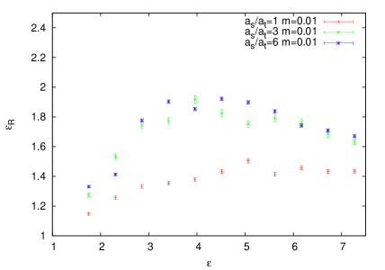
Figure 1: The dielectric permittivity of graphene $\epsilon_{R}$ as a function of the dielectric permittivity of substrate $\epsilon$ for different $a_{s}/a_{t}$ at $T=0.23eV(a_{s}T=0.00019)$.

To measure the potential, $V(r)$, between static charges, we calculate the correlator of two Polyakov lines $\langle P^{\gamma}(0)(P^{\gamma}(\vec{r}))^{+}\rangle$:

$$\langle P^{\gamma}(0)(P^{\gamma}(\vec{r}))^{+}\rangle=a\exp{\biggl{(}-\frac{V(\vec{r})}{T}\biggr{)}}.$$ (7)

where $T$ is the temperature of graphene sample, the Polyakov line $P(\vec{r})$ is

$$P(\vec{r})=\exp{\bigl{(}-ie\int_{0}^{1/T}dtA_{0}(t,\vec{r})\bigr{)}}=\prod_{t=0}^{L_{t}-1}\exp{(-i\theta_{(t,\vec{r}),0})}$$ (8)

To suppress statistical errors, we measure the correlator of Polyakov lines in some rational power. Physically this means that the interaction potential between static charges $\pm e\cdot\gamma$ is considered. We have found that for $\gamma\sim 0.1$ the uncertainty of the calculation is much smaller than that in the case of $\gamma=1$ (usual Polyakov line). Below the value $\gamma=0.1$ is used.

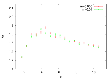
Figure 2: The dielectric permittivity of graphene $\epsilon_{R}$ as a function of the $\epsilon$ for the fermion masses $m=0.005,~{}0.01$ at $T=0.23eV(a_{s}T=0.00019)$.

Below we use the following notations:

$$\alpha_{0}=e^{2}\frac{2}{\epsilon+1}$$ (9)

is the bare effective charge and

$$\alpha_{R}=\frac{\alpha_{0}}{\epsilon_{R}}$$ (10)

is the effective charge, renormalized due to interaction, $\epsilon_{R}$ is effective dielectric permittivity of graphene.

III Numerical results and discussion

III.1 The interaction potential at low temperatures

To get the potential between static charges, we measure the correlator of Polaykov lines and fit $V(r)$ by lattice screened Coulomb potential:

$$V(\vec{r}) = \frac{1}{\epsilon_{R}}V_{C}(\vec{r})+c,$$ (11)

$$V_{C}(\vec{r}) = -\alpha_{R}\frac{\pi\gamma^{2}}{L_{s}^{3}a_{s}}\sum_{n_{1},n_{2},n_{3}}\frac{1}{\sum_{i}\sin^{2}(p_{i}a_{s}/2)}e^{i\vec{p}\vec{r}},~{}$$ (12)

$$p_{i} = \frac{2\pi}{L_{s}a_{s}}n_{i}.$$

and determine $\epsilon_{R}$. In formula (12) $c$ is the constant, which parameterizes selfenergy contribution to the potential, $V_{C}(\vec{r})$ is the lattice Couloumb potential, which takes into account spatial discretization and finite volume effects, $n_{i}$ are integers which run in the interval $(0,L_{s}-1)$ and point $n_{1}=n_{2}=n_{3}=0$ is excluded.

Firstly we discuss the systematic errors due to the temporal discretization. Using the algorithm described above we generated $100$ statistically independent gauge field configurations at the lattices $20^{3}\times L_{t},L_{t}=20,60,120$ for a set of values of the dielectric permittivity of substrate $\epsilon\in(1,8)$. These three lattices correspond to the temperature $T=0.23eV(a_{s}T=0.00019)$ and the ratios $a_{s}/a_{t}=1,3,6$ correspondingly. We have found an excellent agreement between our data and expression (12) ($\chi^{2}/dof\sim 1$ for all $\epsilon$). Thus this result confirms that static charges at low temperature in graphene interact via Coulomb potential.

The dielectric permittivity of graphene $\epsilon_{R}$ as a function of the dielectric permittivity of substrate $\epsilon$ for different $a_{s}/a_{t}$ is shown in Fig. 1. From this plot one sees that there is large difference between the results obtained at $a_{s}/a_{t}=1$ and $a_{s}/a_{t}=3$. At the same time the results for $a_{s}/a_{t}=3$ and $a_{s}/a_{t}=6$ are in a reasonable agreement with each other. It seems that at $a_{s}/a_{t}\sim 3-6$ one approaches to the continuum limit in the temporal direction. Below $a_{s}/a_{t}=6$ discretization scheme is used.

Now let us turn to the fermion mass dependence of our results. In Fig. 2 $\epsilon_{R}$ as a function of the $\epsilon$ for the fermion masses $m=0.005,0.01$ is shown. Within the uncertainty of the calculation the results obtained for different masses are compatible to each other. The simulation of the gauge field configurations with the mass $m=0.005$ is much more time consuming as compared to the mass $m=0.01$. So, to decrease the time of the calculation, all calculations are carried out for the fermion mass $m=0.01$. In addition to the fermion mass dependence, we studied the volume dependence of our results and found that this dependence is very weak.

In Fig. 3 we show how $\alpha_{R}$ is renormalized due to the interaction.

Figure 3: The renormalized charge squared $\alpha_{R}$ as a function of the bare charge squared $\alpha_{0}$ rescaled by the $v_{F}$ and the plot of one loop formula (13). The insulator-semimetal phase transition takes place at $\alpha_{0}/v_{F}\sim 0.9$.

In the semimetal phase the effective coupling constant is not large $\alpha_{0}/v_{F}<1$ and one can try to apply perturbation theory to disribe our data. At one loop approximation the dependence of $\alpha_{R}$ on the $\alpha_{0}$ for graphene is given by the expression Gonzalez:1993uz

$$\frac{\alpha_{R}}{\alpha_{0}}=\frac{1}{1+\frac{\pi}{2}\frac{\alpha_{0}}{v_{F}}}=\frac{1}{1+3.4\frac{2}{\epsilon+1}}.$$ (13)

Fig. 3 shows that at small $\alpha_{0}$ we have good agreement with perturbation theory.

III.2 The temperature dependence of the interaction potential

To study the dependence of the dielectric permittivity $\epsilon_{R}$ on the temperature, we generated $100$ statistically independent gauge field configurations at the lattices $20^{3}\times L_{t},L_{t}=$56, 50, 38, 28, 26, 22, 18. These lattices correspond to the temperatures $T=0.50$ eV ($a_{s}T=0.00041$), $T=0.56$ eV ($a_{s}T=0.00046$), $T=0.74$ eV ($a_{s}T=0.00061$), $T=1.00$ eV ($a_{s}T=0.00082$), $T=1.08$ eV ($a_{s}T=0.00089$), $T=1.28$ eV ($a_{s}T=0.00105$), $T=1.56$ eV ($a_{s}T=0.00128$) correspondingly.

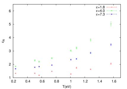
Figure 4: The dependence of the $\epsilon_{R}$ on the temperature of graphene sample for the $\epsilon=1.8$ (insulator phase), $\epsilon=4.0$ (transion region), $\epsilon=7.3$ (semiconductor phase), is shown

In Fig. 4 the dependence of the $\epsilon_{R}$ on the temperature of graphene sample for different dielectric permittivities of substrate $\epsilon$ is shown. Graphene with $\epsilon=1.8$ is in the insulator phase. It is seen that the temperature dependence in this phase is the weakest as compared to the $\epsilon=4.0$ and $\epsilon=7.3$ points. This happens since in the insulator phase fermions have dynamically generated mass. If this mass is larger than the temperature, the production of free charges which enhances the $\epsilon_{R}$ is suppressed. If the fermions are massless, free charges production is no longer suppressed and the temperature dependence of the $\epsilon_{R}$ is stronger. This effect is seen in the semimetal phase at $\epsilon=7.3$, where quasiparticles are massless. The most rapid temperature dependence takes place for $\epsilon=4.0$ which is in the transition region. In this region graphene is in the insulator phase at low temperature and in the semimetal phase at high temperature what explains the most rapid temperature dependence. In Fig. 5 the dependence of $\epsilon_{R}$ on $\epsilon$ at different temperatures is shown.

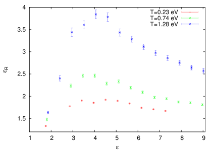
Figure 5: The dependence of the $\epsilon_{R}$ on the $\epsilon$ at different temperatures obtained from the fitting with Coulomb potential $V_{C}(\vec{r})$ (12).

Formula (12) fits data satisfactory ( $\chi^{2}/dof\sim 1-3$ ) for all temperatures. However, the larger the temperature the larger $\chi^{2}/dof$. One can assume that the worsening of the fitting model can be assigned to the following fact. At sufficiently large temperature graphene contains equal number of electrons and holes. If one puts electric charge to such media, a nonzero charge density is created. This charge density leads to some sort of Debye screening in graphene which is not accounted in (12).

In Appendix A the derivation of the Debye screening in graphene is given. It is assumed that the interaction between quasiparticles is weak, which is the case only for sufficienty large $\epsilon$. However, the Debye potential (21) without explicit expression for Debye screening mass $m_{D}$ (22) can be thought of as a modification of the Coulomb potential with unknown parameter $m_{D}$. In this sence formula (21) can be applied for all values of $\epsilon$ and temperature.

To carry out the study of the temperature dependence of the interaction potential we replace the lattice Coulomb potential $V_{C}(\vec{r})$ by the lattice version of Debye screening potential (25) in model (12). Before the modifications of the potential the description ($\chi^{2}/dof>1-3$) of the available data was not as good as it became after the modification ( $\chi^{2}/dof<1$ ) for all temperatures and $\epsilon$. In Fig. 6 we plot the $\epsilon_{R}$ as a function of the $\epsilon$ for different temperatures. It is seen from this plot that contrary to the fitting procedure with Coulomb potential the $\epsilon_{R}$ with Debye screening potential is almost temperature independent. So, the fitting with Debye screening potential cancels the temperature dependence from the dielectric permittivity $\epsilon_{R}$ and encodes it into Debye mass $m_{D}$. This confirms that in some region the temperature dependence of the interaction potential results from the Debye screening.

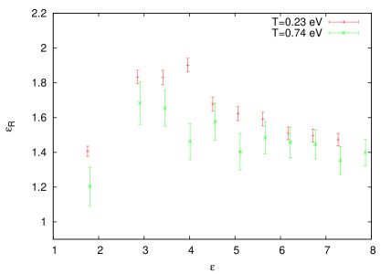
Figure 6: The dependence of the $\epsilon_{R}$ on the $\epsilon$ at different temperatures obtained from the fitting with Debye screening potential $V_{D}(\vec{r})$ (25).

Now let us turn to Debye screening mass. Equation (24) defines the Debye mass for two-dimensional plasma of quasiparticles when interaction between quasiparticles is disregarded. It not difficult do derive the expression for Debye mass $m_{D}$ which is valid for the interacting quasiparticles. Evidently, if there is no interaction between quasiparticles, $m_{D}=0$. This means that the expansion of $m_{D}$ starts for the term proportional to the $\sim\alpha_{R}$, which determines the strength of the interaction. The second property of the $m_{D}$ is that it disappears if the density of quasiparticles $n$ is zero. So, one concludes that $m_{D}\sim n/T$, where temperature appeared in the denominator for the dimensional reasons. Now we have the following expression

$$m_{D}=k(e^{2},T)~{}{\alpha_{R}}\frac{n}{T},$$ (14)

where $k(e^{2},T)$ is some function which could depend on the $e^{2}$ and $T$. In Fig. 7 we present the following observable $r=(m_{D}e^{2})/(T\alpha_{R})$ which is proportional to the $n/T^{2}$. This observable allows to study the density of quasiparticles in graphene. If the interaction between quasiparticles is weak, the ratio $(m_{D}e^{2})/(T\alpha_{R})$ equals to

$$r=\frac{m_{D}e^{2}}{T\alpha_{R}}=8\log 2\frac{e^{2}}{v_{F}^{2}}\simeq 3600.$$ (15)

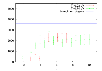
Figure 7: The dependence of the ratio $r=(m_{D}e^{2})/(T\alpha_{R})$ on the $\epsilon$ at different temperatures. The line parallel to the $\epsilon$-axis is the value of the ratio $(m_{D}e^{2})/(T\alpha_{R})$ at the approximation of weakly interacting two-dimensional plasma of quasiparticles.

In Fig.7 the dependence of the ratio $(m_{D}e^{2})/(T\alpha_{R})$ on the $\epsilon$ at different temperatures is shown. The line parallel to the $\epsilon$-axis is the value of the ratio $(m_{D}e^{2})/(T\alpha_{R})$ (15).

Now few comments are in order

• First let us consider the semimetal phase $\epsilon>5$. In this region the ratio $(m_{D}e^{2})/(T\alpha_{R})$ tends to some constant value and this value is by a factor $\sim 1.5-2.0$ smaller than that given by formula (15). The possible source of this disagreement is that in formula (15) we used the bare Fermi velocity $v_{F}$. Evidently one should use the renormalized Fermi-velocity $v_{F}^{R}$, which beyond the scope of this paper. The $v_{F}^{R}$ is larger than the $v_{F}$, so the inclusion of Fermi velocity renormalization will push the constant (15) to the correct direction. Accounting this fact one can conclude that within the uncertainty of the calculation in the semimetal phase electron excitations in graphene form a weakly interacting two-dimensional plasma.

• Assuming that the difference between constant (15) and the position of the plateau in Fig. 7 results from Fermi velocity renormalization one can estimate the ratio $v_{F}^{R}/v_{F}$ in the semimetal phase as $\sim 1.2-1.4$. This value is in a reasonable agreement with the results obtained within Monte-Carlo simulation of graphene Drut:2013wqa and with experiment exp .

• It is seen from Fig. 7 that at low temperature Debye mass $m_{D}$ plays a role of order parameter of the insulator-semimetal phase transition. At small dielectric permittivity of substrate, $m_{D}$ equals zero within the accuracy of the calculation, what means that the interaction potential is Coulomb. At $\epsilon\sim 4-5$ Debye mass becomes nonzero, abruptly reaching the regime of two-dimesional plasma. The interaction in this region is due to Debye potential. Thus the study of Debye screening mass allows to determine the position of the insulator-semimetal phase transition, which takes place at $\epsilon\sim 4-5$, in accordance with the results of papers Lahde:09:1 ; Buividovich:2012uk . At large temperatures $m_{D}$ is not zero for any values of the $\epsilon$. It is smoothly rising function of $\epsilon$ which is saturated at $\epsilon\sim 4-5$.

• To understand the behaviour of the Debye mass, which is proportional to the density of excitations $n$, one can use the following model. In the insulator phase $\epsilon<4$ the fermion excitation acquire dynamical mass. So, the density of charged fermion excitations is exponentially suppressed

  $$\frac{n}{T^{2}}\sim\exp{\biggl{(}-\frac{M_{f}(g^{2})}{T}\biggr{)}}.$$ (16)

  The dynamical fermion mass $M_{f}(g^{2})$ depends on the effective coupling constant $g^{2}=\alpha_{0}/v_{F}$. It is seen from Fig. 7 that at temperature $T=0.23eV(a_{s}T=0.00019)$ the density is either considerably suppressed or equal to zero, what implies that $M_{f}(g^{2})>T$. However, at temperature $T=0.74eV(a_{s}T=0.00061)$ the density is no longer suppressed and it is monotonically rising function of the effective constant, what implies that $M_{f}(g^{2})<T$. So, the dynamically generated fermion mass in the insulator region can be estimated as $M_{f}(g^{2})\sim 0.5eV$.

At the end of this section it worth to note that because of the smallness of the Fermi velocity $v_{F}$ Debye screening radius is rather small. For instance, according to formula (22) for the room temperature and $\epsilon\sim 5$ the screening radius is only $\sim 20\times$distance between carbon atoms in graphene.

In conclusion, in this paper we carried out the study of the interaction potential between static charges in graphene within Monte-Carlo simulation for different dielectric permittivities of substrate $\epsilon$ and various temperatures. To calculate the interaction potential we measured the correlator of Polyakov lines. At low temperatures the interaction can be satisfactory described by the Coulomb potential screened by some dielectric permittivity $\epsilon_{R}$. We determined the dependence of the $\epsilon_{R}$ on the dielectric permittivity of substrate. In addition, we determined the dependence of the renormalized charge squared $\alpha_{R}$ on the bare one $\alpha_{0}$ and showed that at in the semimetal phase the $\alpha_{R}$ can be well described by one loop formula.

At larger temperatures the interaction potential deviates from Coulomb. The main result of this paper is that for all temperatures and dielectric permittivities the interaction can be well desribed by the potential of Debye screening of two-dimensional plasma of fermion excitations. It is shown that at low temperature Debye mass $m_{D}$ plays a role of order parameter of the insulator-semimetal phase transition. At small dielectric permittivity of substrate, $m_{D}$ equals zero within the accuracy of the calculation, what means that the interaction potential is Coulomb. At $\epsilon\sim 4-5$ Debye mass becomes nonzero, abruptly reaching the regime of two-dimensional plasma. The interaction in this region is due to Debye potential. Thus the study of Debye screening mass allows to determine the position of the insulator-semimetal phase transition, which takes place at $\epsilon\sim 4-5$. At large temperatures $m_{D}$ is not zero for any values of the $\epsilon$. It is smoothly rising function of $\epsilon$ which is saturated at $\epsilon\sim 4-5$. In the semimetal phase for all temperatures studied in this paper Debye mass can be rather well described by the formula for two-dimensional plasma of fermions excitations, where the interactions between excitations are accounted by the renormalization of the charge squared $\alpha_{R}$ and the Fermi velocity $v_{F}^{R}$.

Appendix A Debye screening in graphene

This section is devoted to the derivation of the potential of Debye screening in graphene. An important difference between graphene and usual three dimensional electromagnetic plasma is that free charges in graphene are two-dimensional. It will be seen below that this property leads to the change of the exponential screening to power screening.

Suppose that positive charge Q is located at the origin of coordinates. It is clear that quasiparticles with positive charge $+e$ repell from the charge Q. The two-dimensional density of positive quasiparticles on graphene plane can be found from Boltzmann distribution

$$n_{+}(r)=n\exp{\biggl{(}-\frac{e\varphi(r)}{T}\biggr{)}},$$ (17)

where $n$ is a density of positive quasiparticles at infinity, $\varphi(r)$ is the potential which is created by the charge $Q$. Analogously, negative quasiparticles attract to the $Q$ and their density on graphene plane $n_{-}(r)$ can be found as follows

$$n_{-}(r)=n\exp{\biggl{(}\frac{e\varphi(r)}{T}\biggr{)}},$$ (18)

Evidently, the charge density at distance $r$ is

$$\rho(r)=e(n_{+}(r)-n_{-}(r))\simeq-2n\frac{e^{2}\varphi(r)}{T}.$$ (19)

In last equation it was assumed that $e\varphi\ll T$. Taking into account nonzero charge density the $\rho(r)$, one can write Maxwell equation

$$-\Delta\varphi+\frac{8\pi ne^{2}}{T}\delta(z)\varphi=4\pi Q\delta^{3}(\vec{r}).$$ (20)

Note that the delta-function $\delta(z)$ in the second term takes into account the fact that the charges are located on the graphene plane $z=0$. The solution of the Maxwell equation on the graphene plane can be written as follows

$$\varphi(r) = Q\int\frac{d^{2}p}{(2\pi)}\frac{e^{i\vec{p}\vec{r}}}{|p|+m_{D}}$$ (21)

$$= \frac{Q}{r}\int_{0}^{\infty}d\xi\frac{e^{-(m_{D}r)\xi}}{(1+\xi^{2})^{3/2}}\xi,$$

$$\frac{m_{D}}{T} = \frac{4\pi e^{2}n}{T}=\frac{2\pi^{2}}{3}\frac{e^{2}}{v_{F}^{2}},$$ (22)

here $\vec{p}=(p_{x},p_{y})$. It should be noted here that one can use Fermi distribution instead of Boltzmann distributions (17), (18)

$$n_{\pm}(r)=\int\frac{d^{2}p}{(2\pi)^{2}}\frac{1}{\exp{\bigl{[}(v_{F}|\vec{p}|\pm e\varphi(r))/T\bigr{]}}+1},$$ (23)

expand them in the ratio $e\varphi(r)/T$ and repeat all the above steps. This leads to the same expression for the potential $\varphi(r)$ (21) but with different Debye mass

$$\frac{m_{D}}{T}=8\log{2}\frac{e^{2}}{v_{F}^{2}},$$ (24)

which is by 15 % smaller than Debye mass in equation (22).

The solution $\varphi(r)$ satisfies the following limits

$$\varphi(r)=\left\{\begin{array}[]{cc}\frac{Q}{r},~{}~{}~{}(rm_{D})\ll 1\\ \frac{Q}{r}\frac{1}{(m_{D}r)^{2}},~{}~{}~{}(rm_{D})\gg 1.\end{array}\right.$$

Thus at large distances Debye screening leads to $\sim 1/r^{3}$ decrease of the potential. It causes no difficulties to write lattice version of the potential (21) on the graphene plane

$$V_{D}(\vec{r})=4\pi e^{2}\sum_{n_{1},n_{2}}\frac{f(p_{1},p_{2})}{1+2m_{D}(L_{s}a_{s})^{2}f(p_{1},p_{2})}e^{i\vec{p}\vec{r}},$$ (25)

$$f(p_{1},p_{2})=\frac{1}{4L_{s}^{3}a_{s}}\sum_{n_{3}}\frac{1}{\sum_{i}\sin^{2}(p_{i}a_{s}/2)},~{}~{}p_{i}=\frac{2\pi}{L_{s}a_{s}}n_{i}.$$

In formula (25) the integers $n_{1}$, $n_{2}$, $n_{3}$ run the values $0,1,..,L_{s}-1$, except the case $n_{1}=n_{2}=0$.

References

- (1) R. Heyrovska, ”Atomic Structures of Graphene, Benzene and Methane with Bond Lengths as Sums of the Single, Double and Resonance Bond Radii of Carbon”, arXiv:0804.4086 (2008).
- (2) G. W. Semenoff, Phys. Rev. Lett. 53, 2449 (1984).
- (3) J. E. Drut and T. A. Lähde, Phys. Rev. Lett. 102, 026802 (2009); Phys. Rev. B 79, 165425 (2009); Phys. Rev. B 79, 241405 (2009); J. E. Drut, T. A. Lähde, and E. Tölö, PoS Lattice2010, 006 (2010); PoS Lattice2011, 074 (2011).
- (4) S. Hands and C. Strouthos, Phys. Rev. B 78, 165423 (2008); W. Armour, S. Hands, and C. Strouthos, Phys. Rev. B 81, 125105 (2010); Phys. Rev. B 84, 075123 (2011).
- (5) P. V. Buividovich, E. V. Luschevskaya, O. V. Pavlovsky, M. I. Polikarpov and M. V. Ulybyshev, Phys. Rev. B 86, 045107 (2012) [arXiv:1204.0921 [cond-mat.str-el]].
- (6) P. V. Buividovich and M. I. Polikarpov, Phys. Rev. B 86, 245117 (2012) [arXiv:1206.0619 [cond-mat.str-el]].
- (7) M. van Schilfgaarde, M. I. Katsnelson, Phys. Rev. B 83, 081409 (2011) [arXiv:1006.2426 [cond-mat.str-el]].
- (8) K. S. Novoselov, A. K. Geim, S. V. Morozov, D. Jiang, Y. Zhang, S. V. Dubonos, I. V. Grigorieva, and A. A. Firsov, Science 306, 666 (2004).
- (9) A. H. Castro Neto, F. Guinea, N. M. R. Peres, K. S. Novoselov, and A. K. Geim, Rev. Mod. Phys. 81, 109 (2009).
- (10) A. K. Geim and K. S. Novoselov, Nature Materials 6, 183 (2007).
- (11) I. Montvay and G. Muenster, Quantum fields on a lattice (Cambridge University Press, 1994).
- (12) T. DeGrand and C. DeTar, Lattice methods for quantum chromodynamics (World Scientific, 2006).
- (13) C. Burden and A. N. Burkitt, Eur. Phys. Lett. 3, 545 (1987).
- (14) J. Gonzalez, F. Guinea, M. A. H. Vozmediano and , Nucl. Phys. B 424, 595 (1994) [hep-th/9311105].
- (15) J. ín E. Drut and T. A. Lähde, arXiv:1304.1711 [cond-mat.str-el].
- (16) G. L. Yu et al., Proc.Nat.Acad.Sci.,110,3285 (2013)