/ + 0 and 1 jet at NLO with the POWHEG BOX interfaced to GoSam and their merging within MiNLO
Abstract:
We present a generator for the production of a Higgs boson in association with a vector boson or (including subsequent decay) plus zero and one jet, that can be used in conjunction with general-purpose shower Monte Carlo generators, according to the POWHEG method, as implemented within the POWHEG BOX framework.
We have computed the virtual corrections using GoSam, a program for the automatic construction of virtual amplitudes. In order to do so, we have built a general interface of the POWHEG BOX to the GoSam package. With this addition, the construction of a POWHEG generator within the POWHEG BOX is now fully automatized, except for the construction of the Born phase space.
Our jet generators can be run with the recently proposed MiNLO method for the choice of scales and the inclusion of Sudakov form factors. Since the production is very similar to production, we were able to apply an improved MiNLO procedure, that was recently used in and production, also in the present case. This procedure is such that the resulting generator achieves NLO accuracy not only for inclusive distributions in jet production but also in production, i.e. when the associated jet is not resolved, yielding a further example of matched calculation with no matching scale.
1 Introduction
Higgs boson production in association with a vector boson ( production from now on) is an interesting channel for Higgs boson studies at the LHC. On one hand, it seems to be the only available channel to study the Higgs branching to , or to set limits to the Higgs branching into invisible particles. In particular, in the process with the Higgs boson decaying into a pair, the CMS experiment has reported an excess of events over the background of 2.2 standard deviation that is consistent with an Higgs boson [1] in the 7 TeV data. The ATLAS experiment is not reporting any excess, but is setting a limit above 1.9 standard deviation from the Standard Model prediction [2]. The CDF and D0 Collaborations have reported evidence for an excess of events, at the 3.1 standard deviation level, in the search for the standard model Higgs boson in the process with the Higgs decaying to [3, 4, 5]. Looking for invisible Higgs boson decays in associated production, the ATLAS experiment is setting 95% confidence level limits on a 125 GeV Higgs boson decaying invisibly with a branching fraction larger than 65%. Searches for have also been carried out by both ATLAS [6] and CMS [7], and the Higgs boson decay into pairs has also been studied [8].
A POWHEG [9] generator for the has been presented in ref. [10], and is often used for simulating the signal in the experimental analysis. It is developed within the HERWIG++ framework [11].
The aim of this paper is twofold:
-
1.
to present generators for the and + 1 jet processes in the POWHEG BOX [12, 13] framework, a next-to-leading order+parton shower (NLO+PS) event generators. In the following we will refer to these generators as HV and HVJ, respectively. These generators can be interfaced with any parton shower compliant with the Les Houches Interface for User Processes [14, 15], like PYTHIA [16], Pythia8 [17], HERWIG [18] and HERWIG++ [11].
-
2.
To illustrate a new interface of the POWHEG BOX to the GoSam [19] package, that allows for the automatic generation of the virtual amplitudes. In order to achieve this, the POWHEG BOX interface to MadGraph4 of ref. [20] was extended to produce also a file that can be passed to GoSam in order to generate the virtual amplitudes. Using this new tool, the generation of all matrix elements is performed automatically, and one only needs to supply the Born phase space in order to build a POWHEG process.
In our + 1 jet generators, we apply the improved version of the MiNLO procedure [21] discussed in ref. [22]. In [22] it was shown that, by applying this procedure to the NLO production of a color-neutral object in association with one jet, one can reach NLO accuracy for quantities that are inclusive in the production of the color-neutral system, i.e. when the associated jet is not resolved. In the present case, the process can be viewed as the production of a virtual vector boson, that decays into the pair, accompanied by one jet. Since vector-boson production was explicitly considered in ref [22], the same MiNLO procedure used in that context can be transported and applied to the present case. The HVJ+MiNLO generator that we build can then replace the HV generator, since it has the same NLO accuracy, and in addition it is NLO accurate in the production of the hardest jet. We are then able to produce a matched calculation, with no matching scale, without actually merging different samples.
In addition to this, it turns out that it is possible to extend the precision of our HVJ+MiNLO generator in such a way to reach next-to-next-to-leading order+parton shower (NNLO+PS) accuracy for inclusive distributions. This can be achieved following the procedure outlined in ref. [22], i.e. by rescaling the HVJ+MiNLO results with the the NNLO calculation for production, already available in the literature [23]. We remind that higher accuracy for the production of an associated jet is particularly useful in contexts where an extra jet is vetoed, like in the search for invisible Higgs boson decays, or, in general, when events are also classified according to the number of jets. In this paper, we will not pursue the extension of our calculation to the NNLO+PS accuracy, postponing a phenomenological study of this to a future publication.
The organization of the paper is the following: in sec. 2 we describe the new GoSam - POWHEG BOX interface. In sec. 3 we give more details about the virtual contribution and in sec. 4 we briefly review the MiNLO procedure for the present case. In sec. 5 we compare the improved HVJ+MiNLO outputs with the HV ones, and discuss a few phenomenological results. Finally in sec. 6 we summarize our findings. Instructions on how to generate a new virtual code using the GoSam - POWHEG BOX interface and how to drive the GoSam program are collected in Appendixes A and B.
2 The GoSam - POWHEG BOX interface
The code for the calculation of the one-loop corrections to production has been generated using GoSam interfaced to the POWHEG BOX. GoSam is a python framework coupled to a template system for the automatic generation of fortran95 codes for the evaluation of virtual amplitudes. The one-loop virtual corrections are evaluated using algebraic expressions of -dimensional amplitudes based on Feynman diagrams. The diagrams are initially generated using QGRAF [24]. GoSam allows to select the relevant diagrams which are processed with FORM [25], using the SPINNEY [26] package. The processing amounts to organize the numerical computation of the amplitudes in terms of their numerators that are functions of the loop momentum. Finally, the manipulated algebraic expressions of the one-loop numerators are optimized and converted into a fortran95 code111This phase in GoSam can be performed by FORM (version 4.0 or higher) or through the JAVA program Haggies [27]. and merged into the code generated by GoSam.
When integrating over the phase space, the virtual matrix elements are evaluated with SAMURAI [28] or, alternatively, with Golem95 [29]. The first program evaluates the amplitude using integrand reduction methods [30] extended to -dimensions [31], whereas the latter allows to compute the same amplitude evaluating tensor-integrals. The interplay of the two reduction strategies is used to guarantee the highest speed for the produced codes, while keeping the required precision for good numerical stability of the results. For the evaluation of the scalar one-loop integrals QCDLoop [32, 33], OneLOop [34] or Golem95C [29] can be used.
2.1 Binoth-Les-Houches-Accord interface
GoSam has an interface to generic external Monte Carlo (MC) programs based on the Binoth-Les-Houches-Accord (BLHA) [35], which sets the standards for the communications among a MC program and a general One-Loop Program (OLP). We developed an interface based on the BLHA for the POWHEG BOX MC program as well, and the computation we present here is its first application. In the following we explain the basic features of this interface.
The communication between MC and OLP in the BLHA has two separate stages: a pre-running phase and a running-time phase [35].
-
1.
In the pre-running phase, during code generation, the MC writes an order file which contains all the basic information about the amplitudes that should be generated and computed by the OLP. Among these there are the powers of the strong and electromagnetic couplings, the type of corrections (i.e. whether the OLP should generate QCD, QED or EW loop corrections), information on the helicity and color treatment (average, sum…), and finally the full list of the partonic subprocesses for which the virtual one-loop amplitudes are required. The OLP reads the order file and generates the needed amplitudes together with the code to evaluate them. Furthermore, information on the generated code are written by the OLP into a contract file, which will be read-in again by the MC at every run. The structure of the contract file is similar to the one of the order file. In the former the requests of the MC, contained in the latter, are either confirmed by an “OK” label, or rejected. This allows to be sure that the requests contained in the order file can be satisfied and the codes are coherent, or to detect potential problems due to misunderstanding of the MC requests by the OLP. On top of this, the list of partonic processes is rewritten in the contract file with a numerical label which uniquely identifies each subprocess. This will be used at running time by the MC to obtain the amplitude of a specific subprocess from the OLP.
-
2.
At running time the MC reads-in once the contract file and then communicate with the OLP via two standard subroutines: the first one is responsible for the initialization of the OLP, whereas the second one is called for the evaluation of the virtual corrections of a specific partonic subprocess at a given phase-space point. As a reply, the OLP provides an array containing the coefficients of the poles and the finite part of the virtual contribution.
We have extended the already existing interface [20] of the POWHEG BOX to MadGraph4 in order to write an order file and read a contract file.
Together with the order file, GoSam needs a further input card: this is a file, called gosam.rc, where the user can specify further details on the generation of the virtual contributions. Among these there are, for example, the number of available cpus or the treatment of classes of gauge-invariant diagrams.
This setup allows for a completely automated generation of all the matrix elements needed by the POWHEG BOX for the computation of the QCD corrections to any Standard Model process. The limitation is, of course, the computing power of nowadays computer.
3 The virtual corrections
In this section we would like to comment on the structure of the virtual diagrams contributing to production.
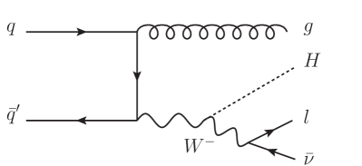
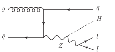
Typical tree-level diagrams for the and production are illustrated in fig. 1. Similar ones can be drawn for real-radiation diagrams. In all these contributions, the Higgs boson is radiated off the vector boson. In fact, we consider all quark to be massless, with the only exception for the top quark, running in fermionic loops.
The virtual corrections can be separated into three different classes:
-
(a)
In the first class, we can accommodate the one-loop Higgs-Strahlung-type diagrams, with no closed fermionic loop.
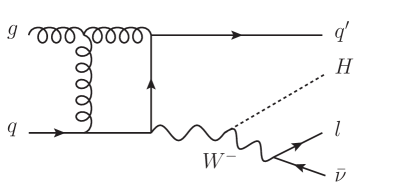
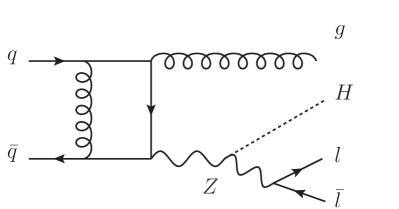
Figure 2: A sample of one-loop Higgs-Strahlung diagrams, with no closed fermionic loop. A sample of diagrams belonging to this class is depicted in fig. 2. These diagrams are similar to the virtual diagrams for production, with the addition of an extra parton in the final state.
-
(b)
A sample of diagrams belonging to the second class of virtual corrections are illustrated in fig. 3.
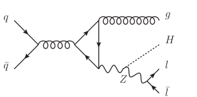
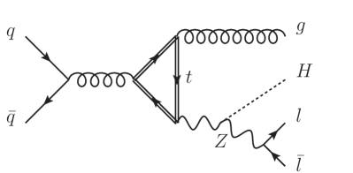
Figure 3: A sample of one-loop Higgs-Strahlung diagrams, with massless and massive closed fermionic loop. In this figure we have plotted Higgs-Strahlung-type diagrams when a closed quark loop is present, and the boson couples to the internal quark. No such diagrams are present for production, since the flavour running in the loop must be conserved. These contributions vanish by charge-conjugation invariance (Furry’s theorem), when they couple to a vector current. For axial currents, they cancel in pairs of up-type and down-type quarks, because they have opposite axial coupling, as long as the loop of different flavours can be considered massless. Thus, the up-quark contribution cancels with the down-quark, and, since we treat the charm as massless, its contribution cancels with the strange one. Only the difference between the diagrams with a massive top quark and a massless bottom quark loop survives.
-
(c)
In the last class, we have the Feynman diagrams where the Higgs boson couples directly to the massive top-quark loop. A sample of this type of diagrams is illustrated in figs. 4 and 5.

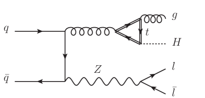
Figure 4: A sample of virtual diagrams involving a massive top-quark loop, where the Higgs boson couples directly to the top quark. 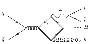
Figure 5: A sample of virtual diagrams involving a massive top-quark loop, where the Higgs boson couples directly to the top quark.
The Feynman diagrams belonging to the three classes are fully implemented in the POWHEG BOX code, and they are computed if the massivetop flag is set to 1 in the input file.
The contributions of the diagrams belonging to classes (b) and (c) are, in general, very small. For example, in production, with the setup described in sec. 5 and with transverse-momentum cuts on jets of 20 GeV, the total NLO cross section, keeping only the virtual diagrams belonging to class (a), is 5.187(4) fb, while keeping all the virtual diagrams is 5.254(4) fb. This behavior is reflected in more exclusive quantities, such as the transverse momentum and rapidity of the pair or of the and bosons.
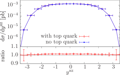
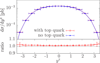
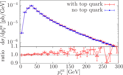
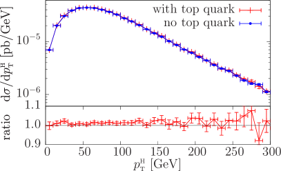
In fig. 6, we compare the rapidity distributions of the system (left plot) and of the boson (right plot), obtained by including the virtual diagrams with the top-quark loop and by neglecting them. In fig. 7 we show a similar comparison for the transverse-momentum distributions of the pair and of the Higgs boson.
In all the several observables that we have examined, we find differences of the order of 1-2%, with the exception of distributions related to the transverse momentum (or of the leading jet ), that display a slightly larger difference increasing with the transverse momentum. Observe that, in this case, our generator would still include correctly the effect of the diagrams of the classes (b) and (c). In fact, the MiNLO correction affects their contribution only at small transverse momentum, where they are negligible (see sec. 4 for more details).
Since the contributions of the diagrams belonging to classes (b) and (c) are at the level of a few percent for inclusive and typical more exclusive distributions, the default behavior of the POWHEG BOX is to neglect them, i.e. the default value of the massivetop flag is 0. We can then apply in a straightforward way the improved MiNLO procedure to production, as illustrated in sec. 4. We would like to point out that the diagrams belonging to classes (b) and (c) not only have a small impact on the cross sections, but they contribute to the differential cross section with terms that are finite, down to zero transverse momentum of the jet, i.e. they do not have the diverging behavior of the diagrams belonging to class (a).
4 The MiNLO procedure
The application of the MiNLO procedure to production is fully analogous to the case of the generator presented in ref. [22], and based on ref. [21], if we keep only the virtual diagrams that belong to class (a), i.e. if the production mechanism is an Higgs-Strahlung one
| (1) |
with no top-quark loop involved.
In the MiNLO method, the NLO inclusive cross section for the computation of the underlying Born kinematics (the so called function in the POWHEG jargon) is modified with the inclusion of the Sudakov form factor and with the use of appropriate scales for the couplings, according to the formula
| (2) |
where is the virtuality of the vector boson before the Higgs-boson emission, i.e. , where and are the momenta of the leptons into which the boson decays, and is the Higgs boson momentum. The transverse momentum of is indicated with . In eq. (2) we have stripped away one power of from the Born (), the virtual () and the real () contribution, and we have explicitly written it in front, with its scale dependence. The scale at which the remaining power of in , and is evaluated and the factorization scale used in the evaluation of the parton distribution functions is again . The Sudakov form factor is given by
| (3) |
and
| (4) |
is the expansion of in powers of . The functions and have a perturbative expansion in terms of constant coefficients
| (5) |
In the improved MiNLO approach, only the coefficients , , and are needed in order to have NLO accuracy also in inclusive distributions. Their value for the case at hand are given by [36, 37, 38]
| (6) | |||||
| (7) | |||||
and the expansion of the Sudakov form factor in eq. (4) is given by
| (8) |
Following the reasoning in ref. [22] we can show that events generated according to eq. (2), i.e. our HVJ-MiNLO generator, are NLO-accurate for distributions inclusive in the production and have NLO accuracy for distributions inclusive in the + 1 jet too.
5 Implementation and plots
In this section we discuss and compare results obtained using the HV and the HVJ-MiNLO generator, as implemented in the POWHEG BOX.
In our study we have generated 5 millions events both for the and for the sample, where is a , a or a boson, which decays leptonically. The conclusions drawn for associated production are similar to those for production. For this reason, in the following, we will show only results for production.
The produced samples were generated for the LHC running at 8 TeV, with GeV and MeV, and with the Higgs boson virtuality distributed according to a fixed-width Breit-Wigner function. In addition, we have restricted the Higgs boson and boson virtuality in the range 10 GeV–1 TeV. This range can be set by the user via the powheg.input file. A minimum transverse momentum cut of 260 MeV has been applied to the jet in the sample in the generation of the underlying Born kinematics, in order to avoid the Landau pole in the strong coupling constant. The factorization scale for the HV POWHEG generators has been set to . The renormalization and factorization scales for the HVJ+MiNLO generators have been set according to the procedure discussed in sec. 4. In our study, we have used the CT10 parton distribution function set [39], but any other set can be used equivalently [40, 41]. The shower has been completed using the PYTHIA shower Monte Carlo program, although it is as easy to interface our results to HERWIG, HERWIG++ and Pythia8. Jets have been reconstructed using the anti- jet algorithms, as implemented in the fastjet package [42, 43] with .
The HV code is run without using the hfact flag, that can be used to separate the real contribution into a singular and a finite part. In the present case, since radiative corrections are modest, we do not expect a large sensitivity to this parameter, as is observed in Higgs boson production in gluon fusion [44, 45]. In the following, the HVJ generator is always run in the MiNLO mode.
| production total cross sections in fb at the LHC, 8 TeV | |||||||
|---|---|---|---|---|---|---|---|
| HWJ-MiNLO | |||||||
| HW | |||||||
| production total cross sections in fb at the LHC, 8 TeV | |||||||
|---|---|---|---|---|---|---|---|
| HZJ-MiNLO | |||||||
| HZ | |||||||
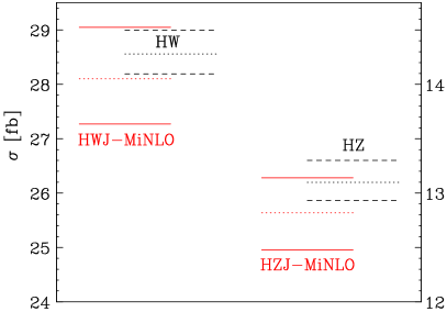
Since the improved MiNLO prescription applied here achieves NLO accuracy for observables inclusive in the production, we begin showing results for the most inclusive quantity, i.e. the total cross section. In tabs. 1 and 2 we collect the results for the total cross sections obtained with the HVJ-MiNLO and the HV programs, both at full NLO level, for different scale combinations. The scale variation in the HVJ-MiNLO results is obtained by multiplying the factorization scale and each of the several renormalization scales that appear in the procedure by the scale factors and , respectively, where
| (9) |
The Sudakov form factor is also changed according to the prescription described in ref. [22]. For ease of visualization, in fig. 8 we have plotted the maximum and minimum values for the HVJ-MiNLO (red lines) and HV (black lines) cross sections in solid and dashed lines, respectively. We have also plotted the central-scale cross section in dotted lines. Notice that we expect agreement only up to terms of higher order in , since the HVJ-MiNLO results include terms of higher order, and also since the meaning of the scale choice is different in the two approaches. For similar reasons, we do not expect the scale variation bands to be exactly the same in the two approaches. From the tables and the figure, it is clear that the standard HV NLO+PS results and the HVJ-MiNLO one are fairly consistent: the HVJ-MiNLO independent scale variation is in general larger than the HV one, and it shrinks if a symmetric scale variations is performed, as illustrated in the last two columns of the tables. In general the HVJ-MiNLO central values are 2% smaller than the HV ones. As already pointed out in ref. [22], comparing full independent scale variation in the HVJ-MiNLO and in the HV approaches does not seem to be totally fair. In fact, in the HV case, there is no renormalization scale dependence at LO, while there is such a dependence in HVJ-MiNLO. It was shown in ref. [22] for the case of production at LO that an independent scale variation corresponds at least in part to a symmetric scale variation in the MiNLO formula. It is thus not surprising that the MiNLO independent scale variation is so much larger than the HV one also at NLO. If we limit ourselves to consider only symmetric scale variations, the MiNLO and the HV results are more consistent, although the HV scale variation band is extremely small.
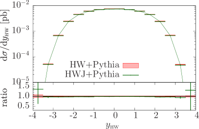
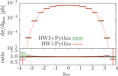
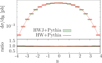
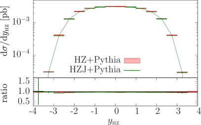
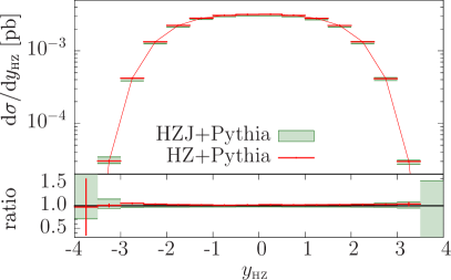
Turning now to less inclusive quantities, we plot in fig. 9 the rapidity distribution of the system obtained with the HW and HWJ-MiNLO generator. We remind that this quantity is predicted at NLO by both generators, and in fact the agreement is very good. The uncertainty band of the HW generator is shown on the left while that of the HWJ-MiNLO generator is shown on the right.
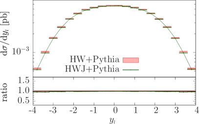
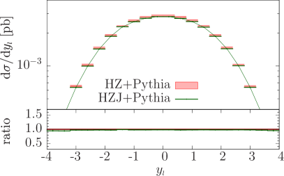
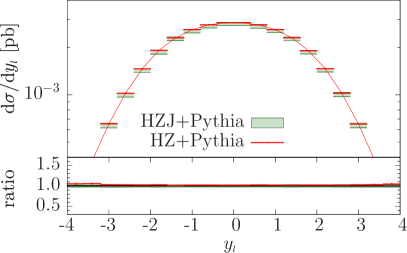
In fig. 10 we show another inclusive quantity, i.e. the charged lepton transverse momentum from the decay. Also in this case we find perfect agreement between the two generators
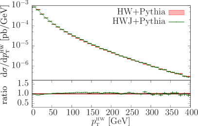
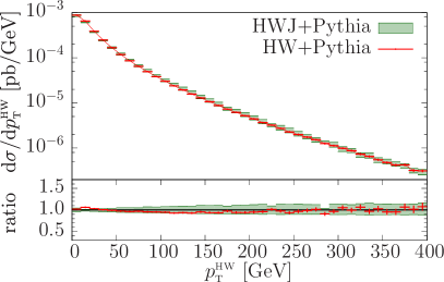
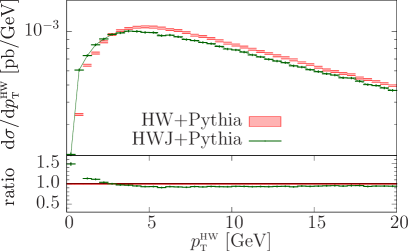
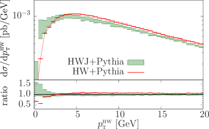
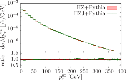
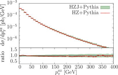
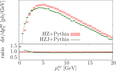
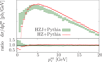
In figs. 11 and 12 we compare the HW and HWJ-MiNLO generators for the transverse momentum of the system. In this case we do observe small differences, that are however perfectly acceptable if we remember that this distribution is only computed at leading order by the HW generator, while it is computed at NLO accuracy by the HWJ-MiNLO generator. It can also be noted that the uncertainty band for the HW generator is uniform, while it depends upon the transverse momentum for the HWJ-MiNLO one. In fact, the uniformity of the scale-variation band in the HW case is well understood: in POWHEG, the scale uncertainty manifests itself only in the function, while the shape of the transverse-momentum distribution is totally insensitive to it.
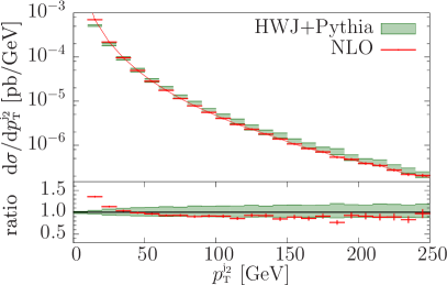
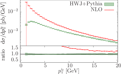
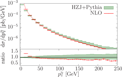
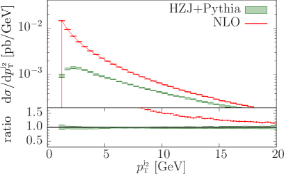
The transverse momentum of the second jet computed with the HWJ-MiNLO generator compared with the pure NLO result is plotted in fig. 13. In this plot, MiNLO plays no role, but the POWHEG formalism is still in place. In fact, the NLO prediction for the second jet has a diverging behavior at low transverse momenta, that is tamed in the POWHEG BOX generator by the Sudakov form factor. Thus, the two results differ considerably from each other, especially at low transverse momenta.
Conclusions similar to those for can be drawn for associated production. For this reason, we refrain from commenting figs. 14–18 that show the same physical quantities shown previously but for production.
6 Conclusions
In this paper we presented new POWHEG BOX generators for and + 1 jet production, with all spin correlations from the vector boson decay into leptons correctly included. The codes for the Born and the real contributions were computed using the existing interface to MadGraph4, while the code for the virtual amplitude was computed using a new interface to GoSam. This interface allows for the automatic generation of the virtual code for generic Standard Model processes. With the addition of this new tool, the generation of all matrix elements in the POWHEG BOX package is performed automatically, and one only needs to supply the Born phase space in order to build a POWHEG process.
We have applied the recently proposed MiNLO procedure to the POWHEG production in order to have a generator that is NLO accurate not only for inclusive distribution in production (as a POWHEG process is) but also in production, i.e. when the associated jet is not resolved. Together with production described in ref. [22], this is a further example of matched calculation with no matching scale.
We have found very good agreement between the HVJ+MiNLO results and the HV ones, for inclusive distributions, while there are clearly differences in the less inclusive distributions, where the HV code has at most leading-order+parton-shower accuracy, while the HVJ one reaches next-to-leading order accuracy.
We point out that, using our HVJ-MiNLO generator, it is actually possible to construct an NNLO+PS generator, simply by reweighting the transverse-momentum integral of the cross section to the one computed at the NNLO level. We postpone a phenomenological study of this method to a future publication.
Acknowledgments
We acknowledge several fruitful discussions with the other members of the GoSam collaboration. The work of G.L. was supported by the Alexander von Humboldt Foundation, in the framework of the Sofja Kovaleskaja Award Project “Advanced Mathematical Methods for Particle Physics”, endowed by the German Federal Ministry of Education and Research. G.L. would like to thank the University of Milano-Bicocca for support and hospitality during the early stages of the work, and the CERN PH-TH Department for partial support and hospitality during later stages of the work.
Appendix A Generation of a new process using GoSam within the POWHEG BOX
In order to generate a new process in the POWHEG BOX using GoSam, the user has to install QGRAF [24], FORM [25], in addition to the GoSam package.
The first step in the generation of the code for a new process is to create a directory under the main POWHEG BOX, and to work from inside this folder, from where all the following script files have to be executed. We will refer to this directory as the process folder. For a complete generation of a new process the following basic steps are needed:
-
•
Generate the tree-level amplitudes and the related code using MadGraph4 [20]. After having copied a MadGraph input card (proc_card.dat) into the process folder, it is sufficient to run from there the BuildMad.sh script contained in the MadGraphStuff folder distributed within the POWHEG BOX. Among the many files generated, this will automatically generate an order file for GoSam.
-
•
Generate the one-loop amplitudes by running the script BuildGS.sh contained in the GoSamStuff folder distributed within the POWHEG BOX with the tag virtual. The script looks for a GoSam input card within the process folder. If no card is found, the user is asked if the template one should be used instead. This command generates all the needed code for the evaluation of the virtual amplitude.
-
•
Generate the interface of the virtual code to the POWHEG BOX. This is done by running again the script BuildGS.sh with the tag interface. This replaces the files init_couplings.f and virtual.f with new ones, containing calls to set the values of the physical parameters and the initialization of the GoSam-generated virtual amplitudes.
The parameters are passed by the POWHEG BOX using the function OLP_OPTION, which is not part of the BLHA standards, but is described in the GoSam manual [46]. The new file virtual.f instead is constructed using the information contained in the contract file, in such a way that the partonic subprocess label assigned by GoSam is not read from the contract file at every run.
-
•
Since the evaluation of the virtual amplitude at running time is performed with SAMURAI and Golem95, both distributed in the GoSam-contrib package, the last step consists in producing a standalone version of everything needed to compute the one-loop amplitudes. This can be achieved by executing a last time the script BuildGS.sh with the tag standalone. The entire code generated by GoSam, together with the code contained in the GoSam-contrib package, is copied in the directory GoSamlib, that is then ready to be compiled together with the rest of the code. The last three steps can be executed all together by running BuildGS.sh with the tag allvirt.
If the generation is successful, the only work left to the user is to provide an appropriate Born phase-space generator in the Born_phsp.f file.
Appendix B The GoSam input card
In this section, we describe the main options of the template GoSam input card available in the directory GoSamStuff/Templates of the POWHEG BOX distribution. Further input options for GoSam can be found in the online manual [46]. There are two categories of input options: one related to the characteristics of the physics process and one more related to the computer code.
B.1 Physics option
We list here the main options related to the physics of the processes. For further options we refer to the GoSam manual.
- model:
-
the first thing to choose is the model needed. By default, GoSam offers the choice among the following three models: sm, smdiag and smehc, which refer to the Standard Model, the Standard Model with diagonal CKM matrix and the Standard Model with effective Higgs-gluon-gluon coupling respectively.
- one:
-
to simplify the algebraic expressions of the virtual amplitudes, a list of parameters can be set algebraically to one using this tag. It will not be possible to change the value of the parameter in the generated code, since the latter will not contain a variable for the corresponding parameter any longer. Due to the normalization conventions used between GoSam and the POWHEG BOX, the virtual amplitudes are always returned stripped off from the strong coupling constant and the electromagnetic coupling , which are therefore set to one using this tag.
- zero:
-
this tag is similar to the previous one and allows to set parameters equal to zero. It is useful to set to zero the desired quark and lepton masses as well as the resonance widths.
- symmetries:
-
this tag specifies some further symmetries in the calculation of the amplitudes. The information is used when the list of helicities is generated. Possible values are:
-
•
flavour: does not allow for flavour changing interactions. When this option is set, fermion lines are assumed not to mix.
-
•
family: allows for flavour-changing interactions only within the same family. When this option is set, fermion lines 1-6 are assumed to mix only within families. This means that e.g. a quark line connecting an up with down quark would be considered, while a up-bottom one would not.
-
•
lepton: means for leptons what “flavour” means for quarks.
-
•
generation: means for leptons what “family” means for quarks.
Furthermore it is possible to fix the helicity of particles. This can be done using the command %<n>=<h>, where stands for a PDG number and for an helicity. For example %23=+- specifies the helicity of all -bosons to be “+” and “-” only (no “0” polarisation).
-
•
- qgraf.options:
-
this is a list of options to be passed to QGRAF. For the complete set of possible options we refer to the QGRAF manual [24]. Customary options which are used are onshell, notadpole, nosnail.
- filter.module, filter.lo, filter.nlo:
-
these tags can impose user-defined filters to the LO and NLO diagrams, passed to GoSam via a python function. Some ready-to-use filter functions are provided by default by GoSam. A complete list can be found in the GoSam online manual. Nevertheless, further filters can be constructed combining existing ones. Ideally, these filters are defined in a separate file, which we call filter.py. The tag filter.module can be used to set the PATH to the file containing the filter.
As an example we report here the filters used for the generation of the codes of the processes presented in this paper, where we want to neglect diagrams in which the Higgs boson couples directly to the massless fermions. Therefore, in a file called filter.py, we define the following filter, selecting diagrams which do not have this vertex:
def no_hff(d):
"""
No Higgs attached to massless fermions.
"""
return d.vertices([H], [U,D,S,C,B], [Ubar,Dbar,Sbar,Cbar,Bbar]) == 0
In the gosam.rc card we can then add the following lines:
filter out filter.module=filter.py
filter.lo= no_hff
filter.nlo= no_hff - extensions:
-
this tag can be used to list a set of options to be applied in the generation of the one-loop code. Among them, the name of the code that will be used in the computation of the diagrams at running time (usually SAMURAI and Golem95), if numerical polarization vectors for external massless vector bosons should be used, if the code should be generated with the option that the Monte Carlo programs controls the numbering of the files containing unstable points…The list of possible extensions useful in conjunction with the POWHEG BOX is:
-
•
samurai: use SAMURAI for the reduction
-
•
golem95: use Golem95 for the reduction
-
•
numpolvec: evaluate polarization vectors numerically
-
•
derive: tensorial reconstruction using derivatives
-
•
formopt: (with FORM 4.0) diagram optimization using FORM (works only with abbrev.level=diagram)
-
•
olp_badpts: (OLP interface only): allows to control the numbering of the files containing bad points from the MC program. This should always be used when generating a code for the POWHEG BOX.
-
•
- PSP_check:
-
this tag switches the detection of unstable points on and off and can take the values true or false.
- PSP_verbosity:
-
the verbosity of the PSP_check can be set here. The possible values are:
verbosity = 0 : no output,
verbosity = 1 : bad points are written in a file stored in the folder BadPoints, which is automatically created in the process folder.
verbosity = 2 : output whenever the rescue system is used with comments about the success of the rescue. - PSP_chk_threshold1, PSP_chk_threshold2:
-
tags to set the threshold used to declare if a point is unstable or not. These thresholds are integers, indicating the number of digits of precision which are required. The first threshold acts on the result given by SAMURAI. If a phase-space point does not fulfill the required precision, it is recomputed using Golem95. The second threshold acts on the result from Golem95. If also the result of Golem95 does not fulfill the required accuracy, the phase-space point and some further information are written in the BadPoints folder, provided the verbosity flag is set.
- PSP_chk_kfactor:
-
a further threshold on the -factor of the virtual amplitude can be set using this tag. If the value is set negative, this tag has no effect and all -factor values are accepted.
- diagsum:
-
to increase the speed of the evaluation of the virtual matrix elements, GoSam can add diagrams which share identical loop-propagators and differ only in the external tree-structure attached to the loop, before the algebraic reduction takes place. This option can be switched on and off by setting this tag to true or false.
- abbrev.level:
-
for an optimal computational speed, during the preparation of the one-loop code, GoSam groups identical algebraic structures into abbreviations. This tag allows to set at which level these abbreviations should be defined. Possible values are helicity, group and diagram. The helicity level is most indicated for easy processes with a small number of diagrams. If the extension formopt is used, the abbrev.level must be set to diagram.
B.2 Computer option
Contrary to a standalone use of GoSam, within the POWHEG BOX framework a separate installation of the gosam-contrib package is not necessary, since this is contained in the POWHEG BOX distribution. The following tags allow to set some options for the external programs:
- qgraf.bin:
-
the location of the QGRAF executable.
- form.bin:
-
the location of the FORM executable. Usually the user can choose between the standard version (form) and the multi-threads version called tform.
- form.threads:
-
when using the multi-thread version of FORM, the number of threads to be used can be set here.
- form.tempdir:
-
the path to the folder where FORM saves temporary files can be set using this tag.
References
- [1] CMS Collaboration Collaboration, Search for the standard model Higgs boson produced in association with or bosons, and decaying to bottom quarks for HCP 2012, CMS-PAS-HIG-12-044.
- [2] ATLAS Collaboration Collaboration, G. Aad et al., Search for the Standard Model Higgs boson produced in association with a vector boson and decaying to a -quark pair with the ATLAS detector, Phys.Lett. B718 (2012) 369–390, [arXiv:1207.0210].
- [3] CDF Collaboration, D0 Collaboration Collaboration, T. Aaltonen et al., Evidence for a particle produced in association with weak bosons and decaying to a bottom-antibottom quark pair in Higgs boson searches at the Tevatron, Phys.Rev.Lett. 109 (2012) 071804, [arXiv:1207.6436].
- [4] CDF Collaboration Collaboration, T. Aaltonen et al., Combined search for the standard model Higgs boson decaying to a bb pair using the full CDF data set, Phys.Rev.Lett. 109 (2012) 111802, [arXiv:1207.1707].
- [5] D0 Collaboration Collaboration, V. M. Abazov et al., Combined search for the standard model Higgs boson decaying to using the D0 Run II data set, Phys.Rev.Lett. 109 (2012) 121802, [arXiv:1207.6631].
- [6] ATLAS Collaboration Collaboration, Search for the Associated Higgs Boson Production in the Decay Mode Using 4.7 fb-1 of Data Collected with the ATLAS Detector at TeV, ATLAS-CONF-2012-078.
- [7] CMS Collaboration Collaboration, Search for SM Higgs in to to , CMS-PAS-HIG-13-009.
- [8] CMS Collaboration Collaboration, Search for the standard model Higgs boson decaying to tau pairs produced in association with a W or Z boson, CMS-PAS-HIG-12-051.
- [9] P. Nason, A new method for combining NLO QCD with shower Monte Carlo algorithms, JHEP 11 (2004) 040, [hep-ph/0409146].
- [10] K. Hamilton, P. Richardson, and J. Tully, A Positive-Weight Next-to-Leading Order Monte Carlo Simulation for Higgs Boson Production, JHEP 04 (2009) 116, [arXiv:0903.4345].
- [11] M. Bahr et al., Herwig++ Physics and Manual, Eur. Phys. J. C58 (2008) 639–707, [arXiv:0803.0883].
- [12] S. Frixione, P. Nason, and C. Oleari, Matching NLO QCD computations with Parton Shower simulations: the POWHEG method, JHEP 11 (2007) 070, [arXiv:0709.2092].
- [13] S. Alioli, P. Nason, C. Oleari, and E. Re, A general framework for implementing NLO calculations in shower Monte Carlo programs: the POWHEG BOX, JHEP 06 (2010) 043, [arXiv:1002.2581].
- [14] E. Boos, M. Dobbs, W. Giele, I. Hinchliffe, J. Huston, et al., Generic user process interface for event generators, hep-ph/0109068.
- [15] J. Alwall, A. Ballestrero, P. Bartalini, S. Belov, E. Boos, et al., A Standard format for Les Houches event files, Comput.Phys.Commun. 176 (2007) 300–304, [hep-ph/0609017].
- [16] T. Sjostrand, S. Mrenna, and P. Z. Skands, PYTHIA 6.4 Physics and Manual, JHEP 0605 (2006) 026, [hep-ph/0603175].
- [17] T. Sjostrand, S. Mrenna, and P. Z. Skands, A Brief Introduction to PYTHIA 8.1, Comput.Phys.Commun. 178 (2008) 852–867, [arXiv:0710.3820].
- [18] G. Corcella, I. Knowles, G. Marchesini, S. Moretti, K. Odagiri, et al., HERWIG 6.5 release note, hep-ph/0210213.
- [19] G. Cullen, N. Greiner, G. Heinrich, G. Luisoni, P. Mastrolia, et al., Automated One-Loop Calculations with GoSam, Eur.Phys.J. C72 (2012) 1889, [arXiv:1111.2034].
- [20] J. M. Campbell, R. K. Ellis, R. Frederix, P. Nason, C. Oleari, et al., NLO Higgs Boson Production Plus One and Two Jets Using the POWHEG BOX, MadGraph4 and MCFM, JHEP 1207 (2012) 092, [arXiv:1202.5475].
- [21] K. Hamilton, P. Nason, and G. Zanderighi, MINLO: Multi-Scale Improved NLO, JHEP 1210 (2012) 155, [arXiv:1206.3572].
- [22] K. Hamilton, P. Nason, C. Oleari, and G. Zanderighi, Merging H/W/Z + 0 and 1 jet at NLO with no merging scale: a path to parton shower + NNLO matching, JHEP 1305 (2013) 082, [arXiv:1212.4504].
- [23] G. Ferrera, M. Grazzini, and F. Tramontano, Associated WH production at hadron colliders: a fully exclusive QCD calculation at NNLO, Phys.Rev.Lett. 107 (2011) 152003, [arXiv:1107.1164].
- [24] P. Nogueira, Automatic Feynman graph generation, J.Comput.Phys. 105 (1993) 279–289.
- [25] J. Kuipers, T. Ueda, J. Vermaseren, and J. Vollinga, FORM version 4.0, Comput.Phys.Commun. 184 (2013) 1453–1467, [arXiv:1203.6543].
- [26] G. Cullen, M. Koch-Janusz, and T. Reiter, Spinney: A Form Library for Helicity Spinors, Comput.Phys.Commun. 182 (2011) 2368–2387, [arXiv:1008.0803].
- [27] T. Reiter, Optimising Code Generation with haggies, Comput.Phys.Commun. 181 (2010) 1301–1331, [arXiv:0907.3714].
- [28] P. Mastrolia, G. Ossola, T. Reiter, and F. Tramontano, Scattering AMplitudes from Unitarity-based Reduction Algorithm at the Integrand-level, JHEP 1008 (2010) 080, [arXiv:1006.0710].
- [29] G. Cullen, J. P. Guillet, G. Heinrich, T. Kleinschmidt, E. Pilon, et al., Golem95C: A library for one-loop integrals with complex masses, Comput.Phys.Commun. 182 (2011) 2276–2284, [arXiv:1101.5595].
- [30] G. Ossola, C. G. Papadopoulos, and R. Pittau, Reducing full one-loop amplitudes to scalar integrals at the integrand level, Nucl. Phys. B763 (2007) 147–169, [hep-ph/0609007].
- [31] R. K. Ellis, W. Giele, and Z. Kunszt, A Numerical Unitarity Formalism for Evaluating One-Loop Amplitudes, JHEP 0803 (2008) 003, [arXiv:0708.2398].
- [32] G. van Oldenborgh, FF: A Package to evaluate one loop Feynman diagrams, Comput.Phys.Commun. 66 (1991) 1–15.
- [33] R. K. Ellis and G. Zanderighi, Scalar one-loop integrals for QCD, JHEP 0802 (2008) 002, [arXiv:0712.1851].
- [34] A. van Hameren, OneLOop: For the evaluation of one-loop scalar functions, Comput.Phys.Commun. 182 (2011) 2427–2438, [arXiv:1007.4716].
- [35] T. Binoth, F. Boudjema, G. Dissertori, A. Lazopoulos, A. Denner, et al., A Proposal for a standard interface between Monte Carlo tools and one-loop programs, Comput.Phys.Commun. 181 (2010) 1612–1622, [arXiv:1001.1307].
- [36] J. Kodaira and L. Trentadue, Summing Soft Emission in QCD, Phys.Lett. B112 (1982) 66.
- [37] C. Davies and W. J. Stirling, Nonleading Corrections to the Drell-Yan Cross-Section at Small Transverse Momentum, Nucl.Phys. B244 (1984) 337.
- [38] C. Davies, B. Webber, and W. J. Stirling, Drell-Yan Cross-Sections at Small Transverse Momentum, Nucl.Phys. B256 (1985) 413.
- [39] H.-L. Lai, M. Guzzi, J. Huston, Z. Li, P. M. Nadolsky, et al., New parton distributions for collider physics, Phys.Rev. D82 (2010) 074024, [arXiv:1007.2241].
- [40] A. D. Martin, W. J. Stirling, R. S. Thorne, and G. Watt, Parton distributions for the LHC, Eur. Phys. J. C63 (2009) 189–285, [arXiv:0901.0002].
- [41] R. D. Ball, V. Bertone, S. Carrazza, C. S. Deans, L. Del Debbio, et al., Parton distributions with LHC data, Nucl.Phys. B867 (2013) 244–289, [arXiv:1207.1303].
- [42] M. Cacciari and G. P. Salam, Dispelling the myth for the jet-finder, Phys.Lett. B641 (2006) 57–61, [hep-ph/0512210].
- [43] M. Cacciari, G. P. Salam, and G. Soyez, The anti- jet clustering algorithm, JHEP 04 (2008) 063, [arXiv:0802.1189].
- [44] S. Alioli, P. Nason, C. Oleari, and E. Re, NLO Higgs boson production via gluon fusion matched with shower in POWHEG, JHEP 0904 (2009) 002, [arXiv:0812.0578].
- [45] S. Dittmaier, S. Dittmaier, C. Mariotti, G. Passarino, R. Tanaka, et al., Handbook of LHC Higgs Cross Sections: 2. Differential Distributions, arXiv:1201.3084.
- [46] http://gosam.hepforge.org/.