A new representation of the Adler function for lattice QCD
Abstract
We address several aspects of lattice QCD calculations of the hadronic vacuum polarization and the associated Adler function. We implement a representation derived previously which allows one to access these phenomenologically important functions for a continuous set of virtualities, irrespective of the flavor structure of the current. Secondly we present a theoretical analysis of the finite-size effects on our particular representation of the Adler function, based on the operator product expansion at large momenta and on the spectral representation of the Euclidean correlator at small momenta. Finally, an analysis of the flavor structure of the electromagnetic current correlator is performed, where a recent theoretical estimate of the Wick-disconnected diagram contributions is rederived independently and confirmed.
pacs:
12.38.Gc, 13.40.Em, 13.66.Bc, 14.60.EfI Introduction
The hadronic vacuum polarization, that is, the way hadrons modify the propagation of virtual photons, is of great importance in precision tests of the Standard Model of particle physics. It enters, for instance, the running of the QED coupling constant. Together with the Higgs mass, the latter can be used to predict the weak mixing angle, which can also be measured directly, thus providing for a test. Secondly, it currently represents the dominant uncertainty in the Standard Model prediction of the anomalous magnetic moment of the muon. Given the upcoming experiment at FermiLab that is expected to improve the accuracy of the direct measurement by a factor 4, it is important to reduce the uncertainty on the prediction by a comparable factor. While the phenomenological determination of the leading hadronic contribution is still the most accurate approach, a purely theoretical prediction is both conceptually desirable and provides for a completely independent check. Since the vacuum polarization is inserted into an integral which is strongly weighted to the low-energy domain, calculating the hadronic vacuum polarization has become an important goal for several lattice QCD collaborations performing non-perturbative simulations Blum (2003); Gockeler et al. (2004); Aubin and Blum (2007); Feng et al. (2011); Boyle et al. (2012); Della Morte et al. (2012a).
One of the features of the numerical lattice QCD framework is that the theory is formulated in Euclidean space of finite extent. Typically the theory is set up on a four-dimensional torus. The limitation of Euclidean correlation functions in finite volume to discrete values of the momenta has drawn considerable attention recently de Divitiis et al. (2012); Aubin et al. (2012); Feng et al. (2013). Many low-energy quantities defined in infinite volume, such as the slope of the Adler function at the origin or the proton radius defined from the slope of its electric form factor at , do not have a unique, canonical definition in finite volume. Instead, different finite-volume representations can be defined, all of which converge to the desired infinite-volume quantity. From the point of view of lattice QCD simulations, a desirable feature of such a representation is that it converges rapidly to the infinite-volume quantity. A different representation can in general be obtained by deriving an equivalent formulation of the infinite-volume quantity, and then carrying it over to the finite-volume theory.
Even if a new representation provides a definition of the vacuum polarization or a form factor for a continuous set of momenta, clearly it only represents progress if the finite-size effect on the final target quantity is reduced. Therefore the merit of a new representation can only be evaluated once some theoretical understanding of the finite-size effects is reached.
Here we explore a representation of the hadronic vacuum polarization based on the time-momentum representation of the vector correlator. The starting point is equation (8), which was previously derived in Bernecker and Meyer (2011). It suggests a way to compute the hadronic vacuum polarization for any value of the virtuality. In this paper we apply the idea in a lattice QCD calculation with two light quark flavors. From the appearance of a power of the time-coordinate in the integral, it is manifest that a derivative with respect to the Euclidean frequency has been taken. With a finite and periodic time extent , the function is not uniquely defined. However, since it is multiplied by a vector correlation function, which falls off exponentially, the ambiguity is parametrically small. How precisely we deal with this issue is presented in section IV.
We address the finite-size effects on our representation of the Adler function in section III. We use the operator product expansion to analyze the finite-size effects at large , and we use the known connection between the finite-volume and the infinite-volume spectral function at low energies to study the finite-size effects at small virtualities. Even if our analysis does not apply to intermediate distances, we expect the finite-size effect coming from the long-distance part of the correlator to be the dominant one. Our results suggest that the slope of the Adler function at the origin is approached from below in the large volume limit.
An important feature of our method is that it applies irrespective of the flavor structure of the current. The method of partially twisted boundary conditions has so far been limited to isovector quantities (see for instance Della Morte et al. (2012a)). Here we present a lattice calculation of the isovector contribution, which allows us to compare our results with those obtained by the commonly used momentum-space method on the same ensemble. The isovector correlator does not require the calculation of Wick-disconnected diagrams, whose standard estimators are affected by a large statistical variance. Recently, a useful estimate of the size of the latter was derived in chiral perturbation theory Juttner and Della Morte (2009); Della Morte and Juttner (2010). Here we revisit this relation, and show that it can be understood in terms of the higher threshold at which the isosinglet channel opens compared to the isovector channel.
During the final stages of this work, a preprint by Feng et al. Feng et al. (2013) appeared with which the present paper has an overlap. The authors of Feng et al. (2013) emphasized the attractive option of accessing the hadronic vacuum polarization at small momenta with a very similar method. They also explored the interesting possibility of analytically continuing the vacuum polarization function into the timelike region below threshold.
II Definitions
In this section we consider QCD in infinite Euclidean space. The vector current is defined as , where the Dirac matrices are all hermitian and satisfy . The flavor structure of the current will be discussed in the next subsection. We use capital letters for Euclidean four-momenta and lower-case letters for Minkowskian four-momenta. In Minkowski space we choose the ‘mostly-minus’ metric convention. In Euclidean space, the natural object is the polarization tensor
| (1) |
and O(4) invariance and current conservation imply the tensor structure
| (2) |
With these conventions, the spectral function
| (3) |
is non-negative for a flavor-diagonal correlator. For the electromagnetic current, it is related to the ratio via
| (4) |
The denominator is the treelevel cross-section in the limit , and we have neglected QED corrections.
Relation (3) can be inverted. The Euclidean correlator is recovered through a dispersion relation,
| (5) |
Finally we introduce the mixed-representation Euclidean correlator
| (6) |
which has the spectral representation Bernecker and Meyer (2011)
| (7) |
The vacuum polarization can be expressed as an integral over Bernecker and Meyer (2011),
| (8) | |||
From here the Adler function is given by
| (9) | |||
The slope of the Adler function at the origin is of particular interest,
| (10) |
For instance, in the case of the electromagnetic current, the hadronic contribution to the anomalous magnetic moment of a lepton is given, in the limit of vanishing lepton mass, by Bernecker and Meyer (2011)
| (11) |
II.1 A note on flavor structure in the theory
For simplicity we consider isospin-symmetric two-flavor QCD. The electromagnetic current is then given by with
| (12) |
For each of these currents , we define polarization tensors as in Eq. (1). Obviously only two are linearly independent, and in particular
| (13) |
A very interesting relation was recently obtained Juttner and Della Morte (2009) between the contributions of the Wick-connected diagrams and the Wick-disconnected diagrams in , similar to Eq. (19) below. The derivation was based on an NLO calculation in chiral perturbation theory (ChPT), and extended to include the strange quark Della Morte and Juttner (2010). Here we rederive the result in a different way without relying on ChPT. In terms of Wick contractions, the Euclidean correlators are given by
| (14) | |||||
| (15) | |||||
| (16) |
where ‘wc’ and ‘wd’ stand for Wick-connected and Wick-disconnected diagrams respectively.
By linearity, spectral functions corresponding to and can be defined as in Eq. (2, 3), although is then not necessarily positive definite. In the isovector channel, the threshold opens at , therefore by Eq. (14), becomes non-zero at the same center-of-mass energy. In the isosinglet channel it opens at ,
| (17) |
In terms of the Wick contractions, this means, from Eq. (15)
| (18) |
In particular, from Eq. (16), the contribution of the Wick-disconnected contribution to the Wick-connected contribution in the electromagnetic current spectral function is given by
| (19) |
This result is exact in two-flavor QCD with isospin symmetry. The derivation shows that it stems essentially from the higher energy threshold at which it becomes possible to produce an isosinglet state. Because experimental data shows that the three-pion channel opens rather slowly (the resonance is very narrow), relation (19) can be expected to be a good approximation at least up to 700MeV. For instance the contribution to the ratio of the channel to the ratio is of order 0.01 at Dolinsky et al. (1991), while the ratio itself lies between 4.0 and 5.0 at the same center-of-mass energy. The smallness of the ratio (19) stems mainly from the small charge factor multiplying the Wick-disconnected contribution in (16).
The relation (18) between the Wick-disconnected and the Wick-connected contribution can be translated back into the Euclidean correlator via the dispersion relation (5). A stronger statement can be made in the time-momentum representation (6), since the low-energy part of the spectral function dominates exponentially at large Euclidean time separations. For we have
| (20) |
Unlike at short distances, where is of order Baikov et al. (2012), the Wick-disconnected diagram is thus of the same order as the Wick-connected diagram at long distances.
The argument just presented can be made for other symmetry channels and can be extended to include the other quark flavors.
III Finite-size effects on the Adler function
In this section we investigate the finite-size effects on the Adler function specifically for the representation (9), although the methods used are more generally applicable.
III.1 Large momenta
We denote by the polarization tensor on an torus to distinguish it from its infinite-volume counterpart , and by the finite-size effect (we will use the same notational convention for other quantities). Although the polarization tensor itself contains a logarithmic ultraviolet divergence, its finite-size effect is ultraviolet finite. When discussing finite-size effects, the specific finite-volume representation used must be specified Bernecker and Meyer (2011). Consider then the Fourier transform of . At large frequency, its finite-size effect is given by the operator product expansion,
| (21) | |||
Dimension-four operators that contribute are the Lorentz scalar, renormalization group invariant operators and , but also the component of the two flavor-singlet, twist-two, dimension-four operators familiar from deep inelastic scattering. The dependence of the Wilson coefficients is logarithmic. The coefficients of the Lorentz scalar operators are known to next-to-leading order Chetyrkin et al. (1985) while the coefficients of the traceless tensor operators are known at leading order Mallik (1998). The latter can be taken from the calculation Mallik (1998) performed for thermal field theory in infinite volume, since on the torus, the expectation value of a traceless rank-two tensor operator only has one independent non-vanishing component in spite of the lack of rotational invariance in a time slice.
We thus see that the relative volume effect on the polarization tensor is suppressed by a factor . Furthermore, the finite-size effect on the expectation value of a local operator appearing in Eq. (21) is of order for sufficiently large . This fact is familiar from finite-temperature QCD. The leading finite-size effect is due to a one-particle state, so that the prefactor of can be related to a pion matrix element Meyer (2009).
The lesson is that for momenta sufficiently large that the Fourier-transformed product of currents can be represented by a local operator, the asymptotic finite-size effects on the polarization tensor are of order . This statement about the finite-size effect on then carries over to the Adler function at large .
III.2 Long-distance contribution to
One of the most important observables is the slope of the Adler function at (which up to a numerical factor coincides with the slope of the vacuum polarization). It determines the leading hadronic contribution to the anomalous magnetic moment of the electron Bernecker and Meyer (2011), and a large fraction of the muon’s anomalous magnetic moment Brandt et al. (2012). It is theoretically attractive, because it involves no energy scale external to QCD. In the representation given in Eq. (10), the dominant contribution comes from Euclidean time separations . We therefore find it useful to define
| (22) |
so that . In the infinite-volume theory, the contribution of the states with an energy up to and including the mass completely dominates this contribution. Given the argument made above on the finite-size effects on the short-distance contribution to the Adler function, and the form of the finite-size effects in free field theory (see section A.3), we expect the finite-size effects on to be dominated by the finite-size effects on for . We are therefore led to discuss the latter. We will only consider the case where the pion mass is set to its physical value, but with a suitable model for the timelike pion form factor , our analysis can be extended to other pion masses.
If a temporal extent is chosen, as is common practice, the dominant finite-size effect comes from the finite spatial box extent. In the following theoretical analysis we therefore set to infinity. How to proceed in practice where is finite is discussed in section (V).
| 1.548 | 0.0737 | 6.606 | 3.507 |
|---|---|---|---|
| 2.133 | 0.4702 | 11.53 | 12.85 |
| 2.559 | 1.1333 | 28.95 | 42.52 |
| 2.831 | 0.7509 | 23.09 | 16.21 |
| 3.171 | 0.1124 | 62.41 | 4.558 |
| 3.581 | 0.1452 | 25.13 | 1.615 |
| 3.912 | 0.1335 | 19.36 | 0.867 |
| 4.459 | 0.0192 | 91.10 | 0.391 |
One source of finite-size effects are the polarization effects on single-particle states. They have been analyzed in detail in the past Luscher (1986). The upshot is that the properties of these states are only affected by corrections that are exponential in the linear torus size. In the following, we will neglect these finite-size corrections. In lattice QCD calculations, this assumption will have to be checked explicitly.
In Bernecker and Meyer (2011), an analysis of the finite-size effects on was carried out using the relation between the finite-volume spectral function and the infinite-volume spectral function Luscher (1991a); Meyer (2011). This relation is only firmly established up to the inelastic threshold of . Here we will be less rigorous and assume that even somewhat above this threshold, the relation remains a good approximation. The main justification for this assumption is that the decays almost exclusively into two pions. We also neglect possible contributions from scattering in the and higher partial waves.
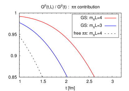
Before using the full machinery of Lüscher’s finite-volume formalism, it is worth understanding the qualitative behavior of in two simple, opposite limits. In one limit, we have non-interacting pions, and can be computed exactly both in finite and in infinite volume. The ratio of the finite-volume to the infinite-volume correlation function is diplayed in Fig. (1). Clearly the finite-size effects are large for a typical value of .
In the other limit, the pion interactions are such that the vector current only couples to a stable meson, . This limit correspond to the expected behavior at very large number of colors . In this case, . The only finite-volume effect in this case stems from the finite-size effects on and , which are exponentially small in the volume. Thus in this limit the finite-size effects are expected to be much more benign.
Experimental data shows that QCD lies somewhere in between these two extremes, but is somewhat closer to the narrow resonance limit. Using the Gounaris-Sakurai parametrization of the timelike pion form factor Gounaris and Sakurai (1968), we have calculated the eight lowest energy-eigenstates for and and their coupling to the isospin current using the results of Luscher (1991a); Meyer (2011), see Table 1. For details of the calculation we refer the reader to appendix A. Together these states saturate the correlator beyond 1fm to a high degree of accuracy. The ratio is displayed in Fig. 1. Although the relative finite-size effect grows rapidly at long distances, for it is of acceptable size at the distances which dominate (compare with Fig. 4). Finally, table 2 gives the finite-size effect on for . With , the effect amounts to , which is a larger effect than is observed for many mesonic observables. We also note that at the heavier quark masses currently studied in the simulations, the is presumably narrower and the finite-size effect for the same value of is therefore smaller.
| GS | free pions | |
|---|---|---|
| 3 | 0.853 | 0.429 |
| 4 | 0.927 | 0.671 |
| 5 | 0.961 | 0.828 |
IV Numerical Setup
In this and the following sections, we describe a numerical implementation of the representation of the vacuum polarization and Adler function given in Eq. (8, 9). In particular, we show how the integral over the time coordinate can be treated without introducing unnecessarily large finite time-extent effects. We restrict ourselves to one value of the light quark mass and one lattice spacing for which we can directly compare the results obtained with the new method to those obtained with the momentum-space method Della Morte et al. (2012b).
All our numerical results were computed on dynamical gauge configurations with two mass-degenerate quark flavors. The gauge action is the standard Wilson plaquette action Wilson (1974), while the fermions were implemented via the O() improved Wilson discretization with non-perturbatively determined clover coefficient Jansen and Sommer (1998). The configurations were generated using the DD-HMC algorithm Luscher (2005, 2007) as implemented in Lüscher’s DD-HMC package CLS (2010a) and were made available to us through the CLS effort CLS (2010b). We calculated correlation functions using the same discretization and masses as in the sea sector on a lattice of size (labeled F6 in Capitani et al. (2012)) with a lattice spacing of fm Capitani et al. (2011) and a pion mass of MeV, so that .
Regarding the flavor structure, we restrict ourselves to the isovector current , normalized as in Eq. (12). On the lattice we implement the correlation function (6) as a mixed correlator between the local and the conserved current,
| (23) |
where
| (24) | |||||
| (25) | |||||
We have renormalized the vector correlator using
| (26) |
with the non-perturbative value of Della Morte et al. (2005). We have not included O() contributions from the improvement term proportional to the derivative of the antisymmetric tensor operator Luscher et al. (1996); Sint and Weisz (1997). A quark-mass dependent improvement term of the form Sint and Weisz (1997) was also neglected. These contributions should eventually be included to ensure a smooth scaling behavior as the continuum limit is taken. Here, our primary goal is to test the method on a single ensemble.
V Numerical results
We begin by analyzing results for the correlator , and then show how the latter can be used to compute the subtracted vacuum polarization and the Adler function.
V.1 Correlator data
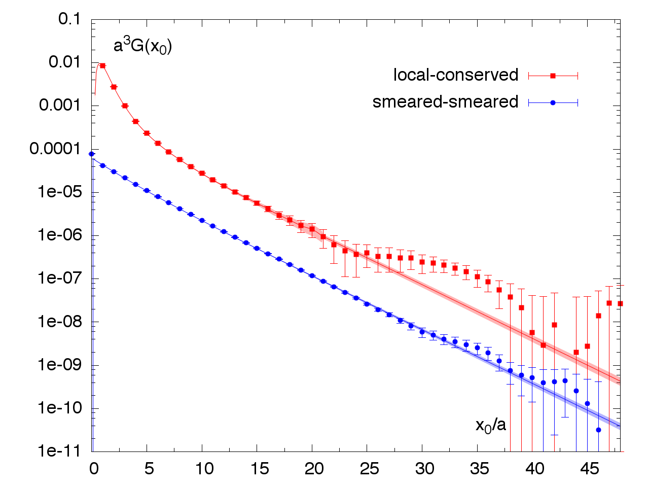
In Fig.2 we show the local-conserved vector correlation function. One virtue of this discretization is that in infinite volume it leads to the property
| (27) |
The correlator must drop to negative values for very small time separations in order to fulfill the above identity. Indeed we observe this negative contact term for very small time separations , and Eq. (27) is satisfied by our data.
The goal is to compute and its derivative from the lattice correlation function using the continuum relation Eq. (8). To achieve this one has to carry out the integral over all time separations. On the lattice this is not straightforward, since only a finite number of points are available. In addition, the signal deteriorates rapidly at large time separations. It is known however that the correlation function decays exponentially for large times. Therefore it is natural to extrapolate the local-conserved correlator with an exponential that decays with the lowest lying ‘mass’111The energy level extracted in this way does not necessarily correspond to a stable vector particle.. This mass can be fixed by fitting the lattice data to an Ansatz of the form
| (28) |
for sufficiently below that the ‘backward’ propagating states make a negligible contribution. To ensure a reliable determination of this mass, we have extracted it from a separate correlation function, computed on the same configurations using smeared operators at the source and sink Capitani et al. (2011). This correlator has greater overlap with the ground state and yields very precise data. The mass parameter determined in this way is then carried over to the local-conserved correlator and the corresponding exponential is smoothly connected to the lattice data by fitting to the data around .
The resulting correlation function is shown as the red shaded band in Fig. 2, where the error estimates were obtained via a jackknife procedure. In the transition region from the data dominated to the extrapolation dominated result the errors increase for a small number of time steps, on the whole however reasonably small errors are achieved in this way.
V.2 Computing and its slope
In order to obtain given the local-conserved correlation function of Fig. 2 one has to compute its convolution with the kernel
| (29) |
Using Eq. (8) derivatives are directly accessible, see for instance Eq. (10).
In Fig. 3 we show the result for and the slope , as computed from the red shaded correlator in Fig. 2. Here all errors were computed using a jackknife method on a total of 392 measurements. Turning first to , for comparison we show the result obtained on the same lattice using the standard method Della Morte et al. (2012b) with the same local-conserved discretization and comparable statistics. The latter method consists in employing Eqs. (1, 2) to obtain first and then determining via extrapolation. In this approach, the number of data points at small was significantly increased using twisted-boundary conditions de Divitiis et al. (2004); Sachrajda and Villadoro (2005); Bedaque and Chen (2005). Still, the extrapolation is difficult to constrain as the signal deteriorates in this limit. The results obtained via Eq. (8) do not suffer directly from these issues, as the physically relevant quantity, , is computed directly.
Clearly the results obtained using our new method are very well compatible with the standard method. It should be noted that the larger errors for large only play a small role when computing , as the large region is highly suppressed in the relevant integral. Using Eq. (9) we also display the slope as a blue shaded band in Fig.3. Throughout the result exhibits small statistical errors and the intercept at can be determined relatively precisely. We find .
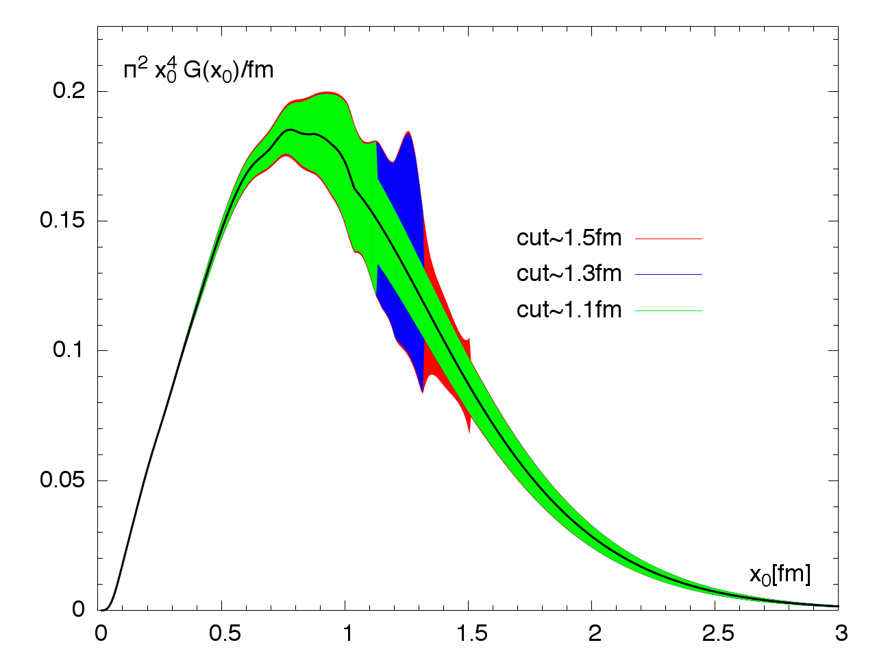
The factor in the integral representation Eq. (10) of the derivative of the Adler function at the origin suppresses the small time region of the correlator. The impact of each -region can be visualized by displaying the integrand, see Fig. 4. Here we also show the results using three different values of the transition point between the data and the extrapolation. This gives us a handle to study the effect of the onset of the fitted pure exponential described above. The effect is seen to lie within the error band, while the impact on the resulting and was checked and found to be negligible. Examining the central value curve we observe that the dominant contribution to the integrand is in fact given by the region 0.5fm1.5fm. Consequently, to precisely pin down and the closely related , very accurate lattice data in this region is desirable.
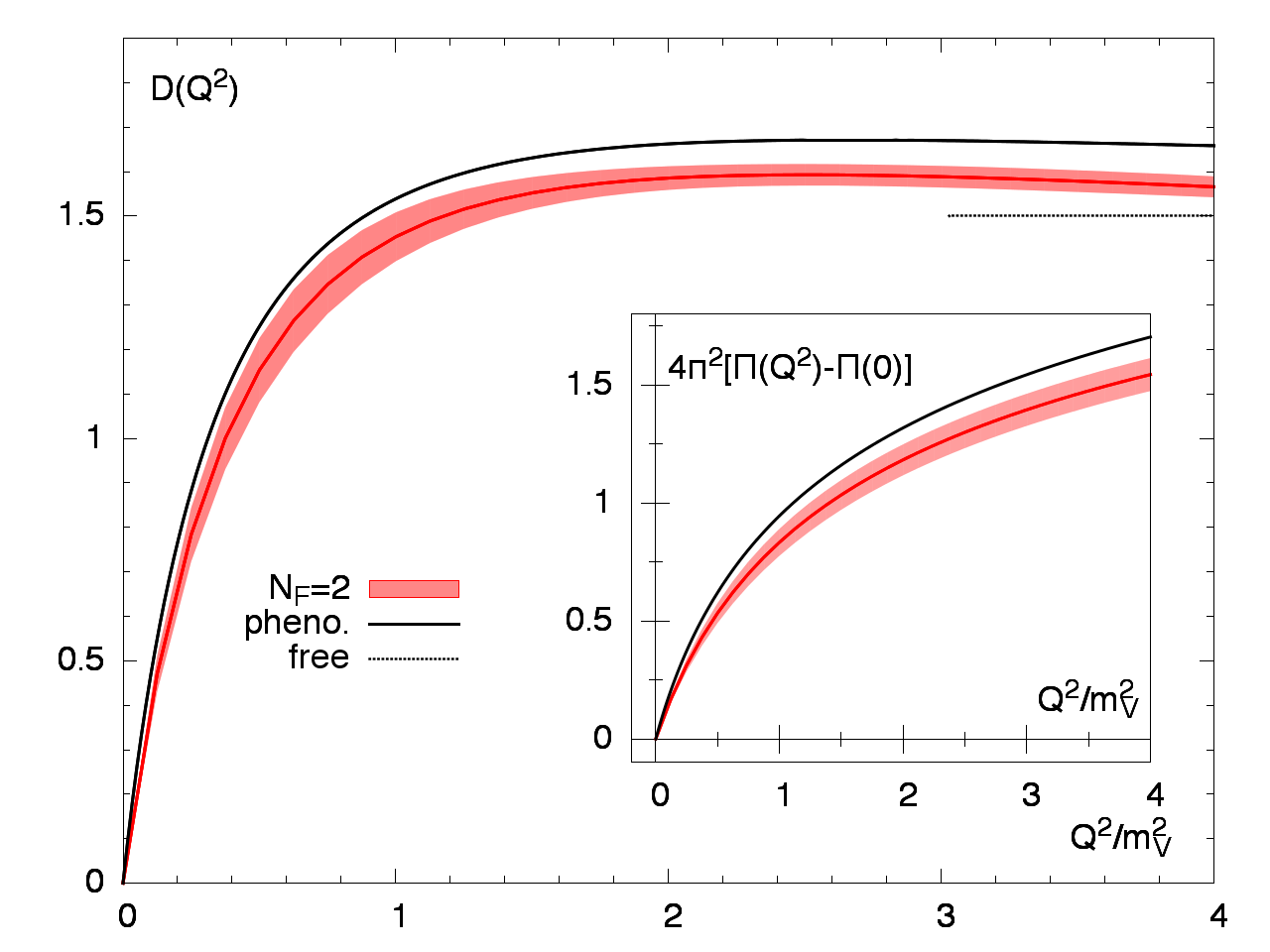
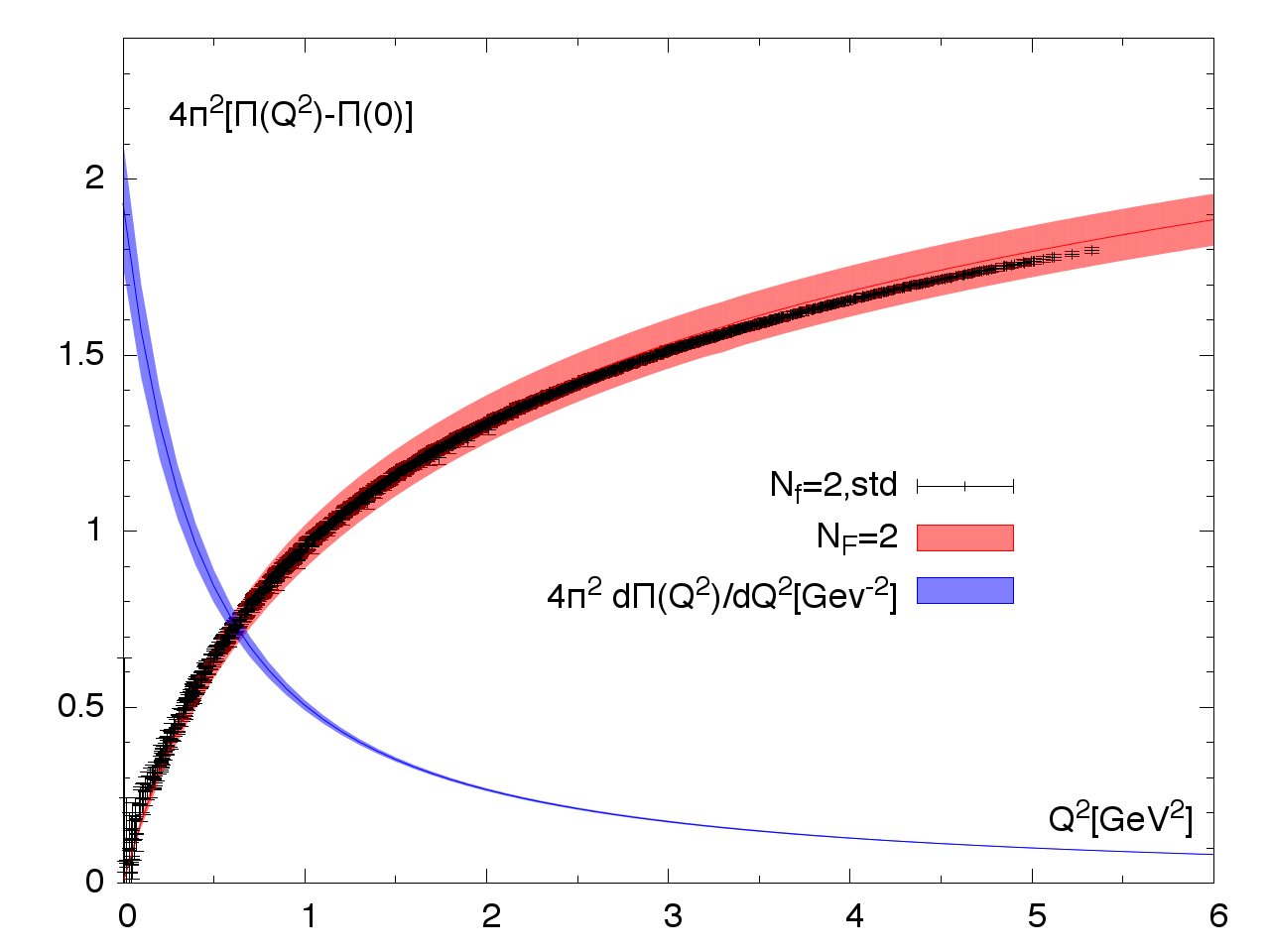
In Fig. 5, where we show the Adler function and the vacuum polarization as a function of the virtuality, we follow the approach Feng et al. (2011); Bernecker and Meyer (2011) of rescaling the horizontal axis using the vector meson mass. In this way one hopes to achieve an approximate scaling at small , in the sense that the curves corresponding to different quark masses approximately lie on top of each other. We compare our result to a phenomenological model (Eq. (93) of Bernecker and Meyer (2011)) for the isovector channel, which predicts in particular . The comparison is shown in Fig. 5 for the low region of and the Adler function . Even after the rescaling, the lattice data lie visibly below the phenomenological curve. A plausible origin for the remaining difference is the spectral density below the mass, since the integrand to obtain is , where is the -ratio restricted to isovector final hadronic states.
VI Conclusion
We have tested a new representation of the vacuum polarization and the Adler function which can be used in lattice QCD (see also Feng et al. (2013)). For the isovector contribution, we have verified that it agrees well with the widely used method in four-momentum space. In the latter case, we have data Della Morte et al. (2012b) generated with twisted boundary conditions, giving access to a discrete but dense set of virtualities. By employing a representation that allows for continuous values of the momenta, it is no more difficult to extract the Adler function than the subtracted vacuum polarization. The former has the advantage of being local in , which facilitates the comparison with perturbation theory at large .
A theoretical analysis of the finite-size effects associated with suggests that the latter can be brought down to about five percent at the physical pion mass for spatial volumes between 4 and 5. The infinite-volume quantity is approached from below. At fixed the finite-size effect depends strongly on the width of the meson, implying that it rapidly becomes a more critical issue when the pion mass is lowered towards its physical value. If the masses and couplings of the low-lying vector states can be determined on the lattice, the bulk of the finite-size effect can be corrected for Bernecker and Meyer (2011).
In the near future we plan to combine the extensive set of data that we have generated with the standard method with the method presented here to extract the Adler function at the origin and . Subsequently, the calculation of the Wick-disconnected diagrams can be taken up with our new representation.
Acknowledgements.
We are grateful to Michele Della Morte and Andreas Jüttner, whose original code formed the basis for our analysis programs, and to our colleagues within CLS for sharing the lattice ensemble used. We thank Georg von Hippel for discussions and for providing the smeared vector correlator Capitani et al. (2011). The correlation functions were computed on the dedicated QCD platform “Wilson” at the Institute for Nuclear Physics, University of Mainz. This work was supported by the Center for Computational Sciences as part of the Rhineland-Palatinate Research Initiative.Appendix A Finite-size effects on the Euclidean correlator
In this appendix we present the details of the calculation that underlies Tables (1, 2) and Figure (1). It is based on the two-pion contribution to the spectral function.
The contribution to the spectral function is given by (see for instance Jegerlehner and Nyffeler (2009))
| (30) |
Charge conservation implies that . Above the threshold , the phase of the pion form factor is equal to the -wave pion phase shift, (Watson theorem).
A.1 Interacting pions
In infinite volume, the Euclidean correlation function is obtained using Eq. (7, 30). For the finite-volume correlator, we proceed as follows.
The discrete energy levels in the box and the infinite-volume phase shifts are related by Luscher (1991b, a)
| (31) | |||
| (32) |
The function , tabulated in Luscher (1991a), is defined by , where is the analytic continuation in of . The corresponding finite volume matrix elements for unit-normalized finite-volume states are given by Meyer (2011)
| (33) | |||||
| (34) |
The correlation function is then obtained as
| (35) |
We thus only need a realistic model for the timelike pion form factor .
A.2 The Gounaris-Sakurai (GS) model of
The GS parametrization Gounaris and Sakurai (1968) contains two free parameters characterizing the resonance, and . Defining via , the phase shift is written
| (36) | |||
| (37) | |||
| (38) |
The form factor is then given by
| (39) | |||||
| (40) |
By analytic continuation, is guaranteed to be unity at the origin. In all numerical applications, we have set , and . These values were chosen so as to approximately match the 2010 KLOE data Ambrosino et al. (2011). We have not tried to correct for isospin breaking effects in the experimental data.
A.3 Non-interacting pions
We consider here the case of non-interacting pions of mass . The isovector current takes the form
| (41) |
for pion fields with a canonically normalized kinetic term. Then one finds in finite volume, with ,
| (42) |
To evaluate the finite-volume correlator at large times, Eq. (42) is an adequate representation. At small times however, it is more efficient to use a different representation obtained using the Poisson formula,
The term coincides with the infinite-volume result, which as a consistency check can also be obtained using Eqs. (7) and (30) by setting . In a saddle point approximation, we have
| (44) | |||
In this form it is clear that for fixed , the expansion converges rapidly as long as is substantially smaller than . Conversely, the finite size effect is exponential for any fixed , but only once is a multiple of . Numerically, if we require that the absolute value of the exponent in the last exponential be at least 4, we get . We also note that the finite-size effect is negative for large .
References
- Blum (2003) T. Blum, Phys.Rev.Lett. 91, 052001 (2003), eprint hep-lat/0212018.
- Gockeler et al. (2004) M. Göckeler et al. (QCDSF Collaboration), Nucl.Phys. B688, 135 (2004), eprint hep-lat/0312032.
- Aubin and Blum (2007) C. Aubin and T. Blum, Phys.Rev. D75, 114502 (2007), eprint hep-lat/0608011.
- Feng et al. (2011) X. Feng, K. Jansen, M. Petschlies, and D. B. Renner, Phys.Rev.Lett. 107, 081802 (2011), eprint 1103.4818.
- Boyle et al. (2012) P. Boyle, L. Del Debbio, E. Kerrane, and J. Zanotti, Phys.Rev. D85, 074504 (2012), eprint 1107.1497.
- Della Morte et al. (2012a) M. Della Morte, B. Jäger, A. Jüttner, and H. Wittig, JHEP 1203, 055 (2012a), eprint 1112.2894.
- de Divitiis et al. (2012) G. de Divitiis, R. Petronzio, and N. Tantalo, Phys.Lett. B718, 589 (2012), eprint 1208.5914.
- Aubin et al. (2012) C. Aubin, T. Blum, M. Golterman, and S. Peris, Phys.Rev. D86, 054509 (2012), eprint 1205.3695.
- Feng et al. (2013) X. Feng, S. Hashimoto, G. Hotzel, K. Jansen, M. Petschlies, et al. (2013), eprint 1305.5878.
- Bernecker and Meyer (2011) D. Bernecker and H. B. Meyer, Eur.Phys.J. A47, 148 (2011), eprint 1107.4388.
- Juttner and Della Morte (2009) A. Jüttner and M. Della Morte, PoS LAT2009, 143 (2009), eprint 0910.3755.
- Della Morte and Juttner (2010) M. Della Morte and A. Jüttner, JHEP 1011, 154 (2010), eprint 1009.3783.
- Dolinsky et al. (1991) S. Dolinsky, V. Druzhinin, M. Dubrovin, V. Golubev, V. Ivanchenko, et al., Phys.Rept. 202, 99 (1991).
- Baikov et al. (2012) P. Baikov, K. Chetyrkin, J. Kuhn, and J. Rittinger, JHEP 1207, 017 (2012), eprint 1206.1284.
- Chetyrkin et al. (1985) K. Chetyrkin, V. Spiridonov, and S. Gorishnii, Phys.Lett. B160, 149 (1985).
- Mallik (1998) S. Mallik, Phys.Lett. B416, 373 (1998), eprint hep-ph/9710556.
- Meyer (2009) H. B. Meyer, JHEP 07, 059 (2009), eprint 0905.1663.
- Brandt et al. (2012) B. Brandt, M. Della Morte, B. Jäger, A. Jüttner, and H. Wittig, Prog.Part.Nucl.Phys. 67, 223 (2012).
- Luscher (1986) M. Lüscher, Commun.Math.Phys. 104, 177 (1986).
- Luscher (1991a) M. Lüscher, Nucl. Phys. B364, 237 (1991a).
- Meyer (2011) H. B. Meyer, Phys.Rev.Lett. 107, 072002 (2011), eprint 1105.1892.
- Gounaris and Sakurai (1968) G. Gounaris and J. Sakurai, Phys.Rev.Lett. 21, 244 (1968).
- Della Morte et al. (2012b) M. Della Morte, B. Jäger, A. Jüttner, and H. Wittig, PoS LATTICE2012, 175 (2012b), eprint 1211.1159.
- Wilson (1974) K. G. Wilson, Phys. Rev. D10, 2445 (1974).
- Jansen and Sommer (1998) K. Jansen and R. Sommer (ALPHA collaboration), Nucl.Phys. B530, 185 (1998), eprint hep-lat/9803017.
- Luscher (2005) M. Lüscher, Comput. Phys. Commun. 165, 199 (2005), eprint hep-lat/0409106.
- Luscher (2007) M. Lüscher, JHEP 0712, 011 (2007), eprint 0710.5417.
- CLS (2010a) http://luscher.web.cern.ch/luscher/DD-HMC/index.html (2010a).
- CLS (2010b) https://twiki.cern.ch/twiki/bin/view/CLS/WebIntro (2010b).
- Capitani et al. (2012) S. Capitani, M. Della Morte, G. von Hippel, B. Jäger, A. Jüttner, et al., Phys.Rev. D86, 074502 (2012), eprint 1205.0180.
- Capitani et al. (2011) S. Capitani, M. Della Morte, G. von Hippel, B. Knippschild, and H. Wittig, PoS LATTICE2011, 145 (2011), eprint 1110.6365.
- Della Morte et al. (2005) M. Della Morte, R. Hoffmann, F. Knechtli, R. Sommer, and U. Wolff, JHEP 0507, 007 (2005), eprint hep-lat/0505026.
- Luscher et al. (1996) M. Lüscher, S. Sint, R. Sommer, and P. Weisz, Nucl. Phys. B478, 365 (1996), eprint hep-lat/9605038.
- Sint and Weisz (1997) S. Sint and P. Weisz, Nucl.Phys. B502, 251 (1997), eprint hep-lat/9704001.
- de Divitiis et al. (2004) G. de Divitiis, R. Petronzio, and N. Tantalo, Phys.Lett. B595, 408 (2004), eprint hep-lat/0405002.
- Sachrajda and Villadoro (2005) C. Sachrajda and G. Villadoro, Phys.Lett. B609, 73 (2005), eprint hep-lat/0411033.
- Bedaque and Chen (2005) P. F. Bedaque and J.-W. Chen, Phys.Lett. B616, 208 (2005), eprint hep-lat/0412023.
- Jegerlehner and Nyffeler (2009) F. Jegerlehner and A. Nyffeler, Phys.Rept. 477, 1 (2009), eprint 0902.3360.
- Luscher (1991b) M. Lüscher, Nucl.Phys. B354, 531 (1991b).
- Ambrosino et al. (2011) F. Ambrosino et al. (KLOE Collaboration), Phys.Lett. B700, 102 (2011), eprint 1006.5313.