Abstract:

Two new optimization techniques based on projections onto convex space (POCS) framework for solving convex and some non-convex optimization problems are presented. The dimension of the minimization problem is lifted by one and sets corresponding to the cost function are defined. If the cost function is a convex function in $R^{N}$ the corresponding set is a convex set in $R^{N+1}$. The iterative optimization approach starts with an arbitrary initial estimate in $R^{N+1}$ and an orthogonal projection is performed onto one of the sets in a sequential manner at each step of the optimization problem. The method provides globally optimal solutions in total-variation, filtered variation, $l_{1}$, and entropic cost functions. It is also experimentally observed that cost functions based on $l_{p},$ $p<1$ can be handled by using the supporting hyperplane concept.

1 Introduction

In many inverse signal and image processing problems and compressing sensing problems an optimization problem is solved to find a solution:

$$\underset{\mathbf{w}\in\text{C}}{\text{min}}f(\mathbf{w})$$ (1)

where $C$ is a set in $\mathbb{R}^{N}$ and $f(\mathbf{w})$ is the cost function. Some commonly used cost functions are based on $l_{1}$, $l_{2}$, total-variation, filtered variation, and entropic functions [1, 2, 3, 4, 5]. Bregman developed iterative methods based on the so-called Bregman distance to solve convex optimization problems which arise in signal and image processing [6]. In Bregman’s approach, it is necessary to perform a D-projection (or Bregman projection) at each step of the algorithm an it may not be easy to compute the Bregman distance in general [7, 8, 5].

In this article Bregman’s projections onto convex sets (POCS) framework [9, 10] is used to solve convex and some non-convex optimization problems instead of his Bregman distance approach. Bregman’s POCS method is widely used for finding a common point of convex sets in many inverse signal and image processing problems[10, 11, 12, 13, 14, 15, 16, 17, 18, 19, 20, 21, 22, 23, 24, 25, 26, 27, 28, 29, 30, 31, 32, 33]. In the ordinary POCS approach the goal is simply to find a vector which is in the intersection of convex sets. In each step of the iterative algorithm an orthogonal projection is performed onto one of the convex sets. Bregman showed that successive orthogonal projections converge to a vector which is in the intersection of all the convex sets. If the sets do not intersect iterates oscillate between members of the sets [34, 35, 36]. Since there is no need to compute the Bregman distance in standard POCS, it found applications in many practical problems.

In our approach the dimension of the minimization problem is lifted by one and sets corresponding to the cost function are defined. This approach is graphically illustrated in Figure 1. If the cost function is a convex function in $R^{N}$ the corresponding set is a convex set in $R^{N+1}$. As a result the convex minimization problem is reduced to finding a specific member (the optimal solution) of the set corresponding to the cost function. As in ordinary POCS approach the new iterative optimization method starts with an arbitrary initial estimate in $R^{N+1}$ and an orthogonal projection is performed onto one of the sets. After this vector is calculated it is projected onto the other set. This process is continued in a sequential manner at each step of the optimization problem. The method provides globally optimal solutions in total-variation, filtered variation, $l_{1}$, and entropic function based cost functions because they are convex cost functions. It is also experimentally observed that cost functions based on $l_{p},$ $p<1$ can be handled by using the supporting hyperplane concept.

The article is organized as follows. In Section 2, the convex minimization method based on the POCS approach is introduced. In Section 3, another convex minimization method based on supporting hyperplanes is studied. Since it is very easy to perform an orthogonal projection onto a hyperplane this method is computationally implementable for many cost functions without solving any nonlinear equations. In Section 4, we present some examples on non-convex minimization.

2 Convex Minimization

Let us first consider a convex minimization problem

$$\underset{\mathbf{w}\in\mathbb{R}^{N}}{\text{min}}f(\mathbf{w})$$ (2)

where $f:\mathbb{R}^{N}\rightarrow\mathbb{R}$ is a convex function.

We increase the dimension by one to define the following sets in $\mathbb{R}^{N+1}$ corresponding to the cost function $f(\mathbf{w})$ as follows:

$$\text{C}_{f}=\{\underline{\mathbf{w}}=[\mathbf{w}^{T}~{}y]^{T}:\mathrm{~{}}y\geq f(\mathbf{w})\}$$ (3)

which is the set of $N+1$ dimensional vectors whose $N+1^{st}$ component $y$ is greater than $f(\mathbf{w})$. We use bold face letters for $N$ dimensional vectors and underlined bold face letters for $N+1$ dimensional vectors, respectively.

The second set that is related with the cost function $f(\mathbf{w})$ is the level set:

$$\text{C}_{s}=\{\underline{\mathbf{w}}=[\mathbf{w}^{T}~{}y]^{T}:~{}y\leq\alpha,~{}\underline{\mathbf{w}}\in\mathbb{R}^{N+1}\}$$ (4)

where $\alpha$ is a real number. Here it is assumed that $f(\mathbf{w})\geq\alpha$ for all $f(\mathbf{w})\in\mathbb{R}$ such that the sets C_f and C_s do not intersect. They are both closed and convex sets in $\mathbb{R}^{N+1}$. Sets C_f and C_s are graphically illustrated in Fig. 1 in which $\alpha=0.$

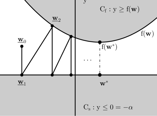
Figure 1: Two convex sets C_f and C_s corresponding to the cost function $f$. We sequentially project an initial vector $\underline{\mathbf{w}}_{0}$ onto $C_{s}$ and $C_{f}$ to find the global minimum which is located at $\mathbf{w}^{*}$.

The POCS based minimization algorithm starts with an arbitrary $\underline{\mathbf{w}}_{0}=[\mathbf{w}_{0}^{T}~{}y_{0}]^{T}\in\mathbb{R}^{N+1}$. We project $\underline{\mathbf{w}}_{0}$ onto the set C_s to obtain the first iterate $\underline{\mathbf{w}}_{1}$ which will be,

$$\underline{\mathbf{w}}_{1}=[~{}\mathbf{w}_{0}^{T}~{}~{}~{}0~{}]^{T}$$ (5)

where $\alpha=0$ is assumed as in Fig. 1. Then we project $\underline{\mathbf{w}}_{1}$ onto the set C_f. The new iterate $\underline{\mathbf{w}}_{2}$ is determined by minimizing the distance between $\underline{\mathbf{w}}_{1}$ and C_f, i.e.,

$$\underline{\mathbf{w}}_{2}=\text{arg}\underset{\underline{\mathbf{w}}\in\text{C}_{\mathrm{s}}}{\text{min}}\|\underline{\mathbf{w}}_{1}-\underline{\mathbf{w}}\|$$ (6)

Eq. 6 is the ordinary orthogonal projection operation onto the set $\mathrm{C_{f}}\in\mathbb{R}^{N+1}$. To solve the problem in Eq. 6 we do not need to compute the Bregman’s so-called D-projection. After finding $\underline{\mathbf{w}}_{2}$, we perform the next projection onto the set C_s and obtain $\underline{\mathbf{w}}_{3}$ etc. Eventually iterates oscillate between two nearest vectors of the two sets C_s and C_f. As a result we obtain

$$\underset{n\rightarrow\infty}{\text{lim}}\underline{\mathbf{w}}_{2n}=[~{}\mathbf{w}^{*}~{}~{}~{}f(\mathbf{w}^{*})~{}]^{T}$$ (7)

where $\mathbf{w}^{*}$ is the N dimensional vector minimizing $f(\mathbf{w})$. The proof of Equation (7) follows from Bregman’s POCS theorem [9, 34]. It was generalized to non-intersection case by Gubin et. al [34, 12],[35]. Since the two closed and convex sets $C_{s}$ and $C_{f}$ are closest to each other at the optimal solution case, iterates oscilate between the vectors $[~{}\mathbf{w}^{*}~{}~{}~{}f(\mathbf{w}^{*})~{}]^{T}$ and $[~{}\mathbf{w}^{*}~{}~{}~{}0~{}]^{T}$ in $R^{N+1}$ as $n$ tends to infinity. It is possible to increase the speed of convergence by non-orthogonal projections [24].

If the cost function $f$ is not convex and have more than one local minimum then the corresponding set $C_{f}$ is not convex in $R^{N+1}$. In this case iterates may converge to one of the local minima. This is graphically illustrated in Fig. 2.

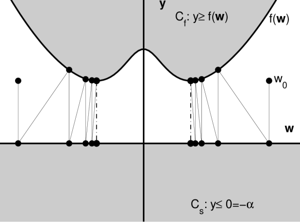
Figure 2: Iterations start with an initial vector $\mathbf{w_{0}}$ and iterates converge to a local minimum by the POCS algorithm.

3 Supporting Hyperplane Concept based POCS Solution

It may not be easy to find the orthogonal projection onto the set C_f for some cost functions $f$. In such cases it is possible to use supporting hyperplanes of the convex set to find the minimum of $f(\mathbf{w})$. The second optimization algorithm is based on making successive orthogonal projections onto the supporting hyperplanes of the set $C_{f}$ instead of the actual set.

The set C_f can be expressed as the intersection of halfplanes whose boundaries are supporting hyperplanes as shown in Fig. 3.

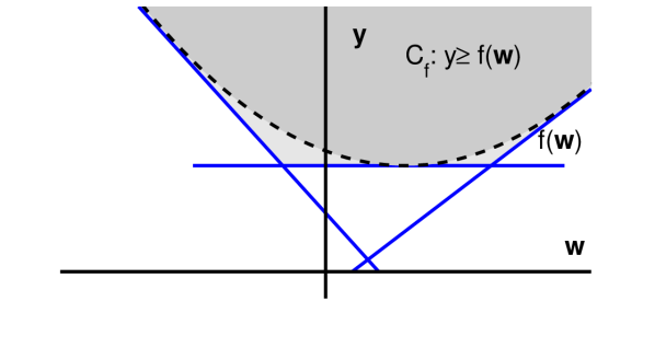
Figure 3: Intersection of supporting halfplanes C_f,w defines the set C${}_{\mathrm{f}}=\bigcap\limits_{\mathbf{w}\in\mathbb{R}}\mathrm{C_{f,\mathbf{w}}}$ when the function f is convex.

Let $\mathbf{w}$ and $f(\mathbf{w})$ form a vector $[\mathbf{w}^{T}f(\mathbf{w})]^{T}$ in $\mathbb{R}^{N+1}$ on the surface of $y=f(\mathbf{w})$. Let the supporting hyperplane at this point be $l(\mathbf{w})$. Let us also define the halfplane (or halfspace) set as follows:

$$\mathrm{C_{f,\mathbf{w}}}=\{y\geq l(\mathbf{w})\}$$ (8)

Clearly, the set C_f can be expressed as the intersection of its supporting halfspaces in $R^{N+1}$:

$$\mathrm{C_{f}}=\bigcap\limits_{\mathbf{w}\in\mathbb{R}^{N}}\mathrm{C_{f,\mathbf{w}}}$$ (9)

Therefore, the POCS approach can be applied to the level set C_s and the family of sets C_f,w, $\mathbf{w}\in\mathbb{R}^{N}$ to find the minimum of $f(\mathbf{w})$. In this case, the number of sets are infinite. This set theoretic scenario was studied by Slavakis, Yukawa, Yamada and Theodoridis [13, 19].

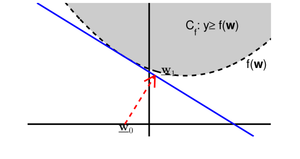
Figure 4: Projection $\underline{w}_{1}$ of the vector $\underline{w}_{o}$ onto a supporting hyperplane

.

In the second optimization approach we perform orthogonal projections onto supporting hyperplanes of the cost function instead of the actual set $\mathrm{C_{f}}$ as shown in Fig. 4. Since making an orthogonal projection onto a hyperplane is easy to compute, the optimization problem does not require the solution of any nonlinear equations as long as it is possible to compute the surface normal at $f(\mathbf{w})$. Let the surface normal at $[\bf{w}_{t}^{T}~{}f(\bf{w}_{t})]^{T}$ be $\bf{v}_{t}\in R^{N+1}$. The supporting hyperplane $l(\bf{\underline{w}}_{t})$ is given by

$$\mathbf{\underline{v}}_{t}^{T}\dot{(}{\underline{\bf{w}}}-{\underline{\bf{w}}}_{t})=0$$ (10)

The orthogonal projection ${\underline{\bf{w}}}_{p}$ of an arbitary vector ${\underline{\bf{w}}}_{o}$ onto the hyperplane $l(\bf{\underline{w}}_{t})$ is obtained as follows

$$\mathbf{\underline{w}}_{p}={\underline{\bf{w}}_{o}}~{}+~{}\lambda~{}\frac{\mathbf{\underline{v}}_{t}^{T}\dot{(}{\underline{\bf{w}}_{o}}-{\underline{\bf{w}}}_{t})}{||\mathbf{\underline{v}}_{t}||^{2}}\mathbf{\underline{v}}_{t}$$ (11)

where $\lambda=1$. The parameter $\lambda$ can be selected between $0<\lambda<2$ as in the normalized LMS algorithm [13]. The parameter $\lambda\neq 1$ case corresponds to non-orthogonal projections. Eq. (11) is the key equation of the supporting hyperplane based optimization approach. In Fig. 7 a graphical illustration of the iterative optimization algorithm is shown.

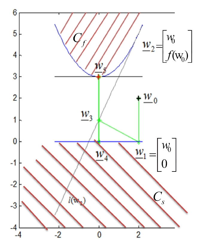
Figure 5: Projections onto supporting hyperplanes of the set $C_{f}$ lead to the global minimum

.

Iterations start with an arbitrary $\underline{\bf{w}}_{o}\in R^{N+1}$. The vector $\underline{\bf{w}}_{o}$ is projected onto the set $C_{s}$ and $\underline{\bf{w}}_{1}$ is obtained. The projected vector is

$$\underline{\bf{w}}_{1}=[{\bf w}_{o}^{T}~{}~{}0]^{T}$$ (12)

where $\bf{w}_{o}$ is an $N$ dimensional vector containing the first $N$ components of the $N+1$ dimensional vector $\underline{\bf{w}}_{o}$. The value of the cost function $f(\bf{w}_{o})$ and its surface normal $\underline{\bf{v}}_{o}$ at $\bf{w}_{o}$ are computed. This is the next iterate

$$\underline{\bf{w}}_{2}=[{\bf w}_{o}^{T}~{}~{}f({\bf w}_{o})]^{T}$$ (13)

The corresponding supporting hyperplane $l(\underline{\bf{w}}_{2})$ is characterized by the equation:

$$\mathbf{\underline{v}}_{o}^{T}\dot{(}{\underline{\bf{w}}}-{\underline{\bf{w}}}_{o})=0$$ (14)

The next iterate $\underline{\bf{w}}_{3}$ is determined by projecting $\underline{\bf{w}}_{1}$ onto the hyperplane $l(\underline{\bf{w}}_{2})$ as follows:

$$\mathbf{\underline{w}}_{3}={\underline{\bf{w}_{1}}}+~{}\lambda~{}\frac{\mathbf{\underline{v}}_{t}^{T}\dot{(}{\underline{\bf{w}}_{1}}-{\underline{\bf{w}}}_{t})}{||\mathbf{\underline{v}}_{o}||^{2}}\mathbf{\underline{v}}_{o}$$ (15)

This computes the first iteration cycle. Next, we project $\mathbf{\underline{w}}_{3}$ onto the set $C_{s}$ and $\underline{\bf{w}}_{4}=[{\bf w}_{3}^{T}~{}~{}0]^{T}$ is obtained. The vector $\bf{w}_{3}$ is an $N$ dimensional vector containing the first $N$ components of the $N+1$ dimensional vector $\underline{\bf{w}}_{4}$. We obtain $\underline{\bf{w}}_{5}=[{\bf w}_{3}^{T}~{}~{}f({\bf w}_{3})]^{T}$ on the surface of the set $C_{f}$. At this point, we verify if $f(\bf w_{3})$ is less than $f(\bf w_{o})$ or not. If yes, we continue the iterations as described above. If not, we switch to another iteration strategy as graphically shown in Fig. 6.

Let us assume that $f(\bf w^{\prime}_{l})>f(\bf w_{l-1})$ as shown in Fig. 6. In this case consecutive iterative projections are performed onto the supporting hyperplanes $l(\bf w^{\prime}_{l})$ and $l(\bf w_{l-1})$ until a vector $[{\bf w}_{l}^{T}~{}~{}f({\bf w}_{l})]^{T}$ satisfying $f(\bf w_{l})>f(\bf w_{l-1})$ is obtained.

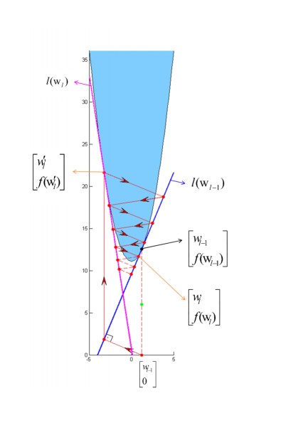
Figure 6: Projections onto two supporting hyperplanes $l(\bf w^{\prime}_{l})$ and $l(\bf w_{l-1})$ to obtain the next iterate satisfying $f(\bf w_{l})>f(\bf w_{l-1})$.

Projection onto a supporting hyperplane is easy to perform. However the cost function may not have a well defined derivative at a given vector ${\bf w}_{u}d$ and a well defined supporting hyperplane may not exist. In this case any hyperplane $l({\bf w_{d}})$ passing through ${\bf w}_{u}d$ and satisfying $f({\bf w})~{}\geq~{}l({\bf w_{d}})$ can be used in Eq. 15.

It is also possible to include other convex constraints into the optimization problem:

$$min~{}~{}f({\bf w})$$ (16)

$$such~{}that~{}{\bf w}\in C_{1},C_{2},\ldots,C_{L}$$

where $C_{1},C_{2},\ldots,C_{L}$ are closed and convex sets representing constraints on the solution of the inverse problem. However the main difficulty with this approach is that non-intersecting multiple convex set scenario has not been fully studied to the best of our knowledge. Successive orthogonal projections onto non-intersecting convex sets may lead to limit cycles [34, 12]. This remains as an interesting research problem. It is experimentally observed that successive orthogonal projections onto $C_{f}$, $C_{s}$ and another constraint set leads to a limit cycle containing the optimal solution.

One possible way to handle the problem described in (3) is to enlarge one or some of the sets so that they have a well defined non-empty intersection. We successfully applied this strategy in FIR filter design [36]. For example, it is trivial to enlarge the set $C_{s}$ by slowly increasing the value of $\alpha$ in a judicuous manner.

It is possible to develop iteration strategies based on non-orthogonal projections or linear combinations of projections to speed up the convergence to the global minimum as discussed in [35, 24, 23].

4 Minimization of Non-Convex Functions

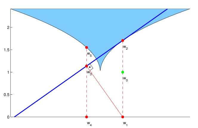
Figure 7: The function $f(w)=|w-2|^{0.5}+1$ is not convex. However projections onto tangential hyperplanes may lead to the global minimum.

An important class of cost functions are based on $l_{p},$ $p<1$. It is experimentally observed that such functions can be minimized by using the ”supporting” hyperplane concept as shown in Fig. 7. Obviously, tangential hyperplanes are no longer ”supporting” hyperplanes and the set $C_{s}$ is not a convex set. This is the ”inside out” version of the convex minimization problem that is studied in Section 3 and the iterative scheme introduced in Section 3 leads to the minimum of the function.

P. Combettes provided an excellent review of POCS theory and the recently introduced proximal splitting method in [35, 37]. The relation between the proposed methods and the proximal splitting theory will be investigated in the future.

Another interesting future research direction is the use of generalized supporting hyperplane concept to minimize non-convex functions with many local minima. The convex hull of the generalized supporting planes may form a convex region in $\mathbb{R}^{N+1}$. As a result it may be possible to find the minimum of the cost function by performing successive orthogonal projections onto generalized supporting hyperplanes. This problem will be also studied in the future.

References

- [1] L. I. Rudin, S. Osher, and E. Fatemi, “Nonlinear total variation based noise removal algorithms,” Physica D: Nonlinear Phenomena, vol. 60, no. 1–4, pp. 259 – 268, 1992. [Online]: http://www.sciencedirect.com/science/article/pii/016727899290242F
- [2] R. Baraniuk, “Compressive sensing [lecture notes],” Signal Processing Magazine, IEEE, vol. 24, no. 4, pp. 118–121, 2007.
- [3] E. Candes and M. Wakin, “An introduction to compressive sampling,” Signal Processing Magazine, IEEE, vol. 25, no. 2, pp. 21–30, 2008.
- [4] K. Kose, V. Cevher, and A. Cetin, “Filtered variation method for denoising and sparse signal processing,” in Acoustics, Speech and Signal Processing (ICASSP), 2012 IEEE International Conference on, 2012, pp. 3329–3332.
- [5] O. Günay, K. Köse, B. U. Töreyin, and A. E. Çetin, “Entropy-functional-based online adaptive decision fusion framework with application to wildfire detection in video,” IEEE Transactions on Image Processing, vol. 21, no. 5, pp. 2853–2865, May 2012.
- [6] L. Bregman, “The Relaxation Method of Finding the Common Point of Convex Sets and Its Application to the Solution of Problems in Convex Programming,” {USSR} Computational Mathematics and Mathematical Physics, vol. 7, no. 3, pp. 200 – 217, 1967. [Online; accessed 03-June-2013]: http://www.sciencedirect.com/science/article/pii/0041555367900407
- [7] W. Yin, S. Osher, D. Goldfarb, and J. Darbon, “Bregman iterative algorithms for -minimization with applications to compressed sensing,” SIAM Journal on Imaging Sciences, vol. 1, no. 1, pp. 143–168, 2008. [Online]: http://epubs.siam.org/doi/abs/10.1137/070703983
- [8] K. Köse, “Signal and Image Processing Algorithms Using Interval Convex Programming and Sparsity,” Ph.D. dissertation, Bilkent University, 2012. [Online; accessed 03-June-2013]: http://signal.ee.bilkent.edu.tr/Theses/kkoseThesis.pdf
- [9] L. Bregman, “Finding the common point of convex sets by the method of successive projection.(russian),” {USSR} Dokl. Akad. Nauk SSSR, vol. 7, no. 3, pp. 200 – 217, 1965. [Online; accessed 03-June-2013]: http://www.sciencedirect.com/science/article/pii/0041555367900407
- [10] D. Youla and H. Webb, “Image Restoration by the Method of Convex Projections: Part 1 Num2014;theory,” Medical Imaging, IEEE Transactions on, vol. 1, no. 2, pp. 81–94, 1982.
- [11] G. T. Herman, “Image Reconstruction from Projections,” Real-Time Imaging, vol. 1, no. 1, pp. 3–18, 1995.
- [12] Y. Censor, W. Chen, P. L. Combettes, R. Davidi, and G. Herman, “On the Effectiveness of Projection Methods for Convex Feasibility Problems with Linear Inequality Constraints,” Computational Optimization and Applications, vol. 51, no. 3, pp. 1065–1088, 2012. [Online; accessed 03-June-2013]: http://dx.doi.org/10.1007/s10589-011-9401-7
- [13] K. Slavakis, S. Theodoridis, and I. Yamada, “Online Kernel-Based Classification Using Adaptive Projection Algorithms,” IEEE Transactions on Signal Processing, vol. 56, pp. 2781–2796, 2008.
- [14] A. Çetin, H. Özaktaş, and H. Ozaktas, “Resolution Enhancement of Low Resolution Wavefields with,” Electronics Letters, vol. 39, no. 25, pp. 1808–1810, 2003.
- [15] A. E. Cetin and R. Ansari, “Signal recovery from wavelet transform maxima,” in IEEE Transactions on Signal Processing, 1994, pp. 673–676.
- [16] A. E. Cetin, “Reconstruction of signals from fourier transform samples,” in Signal Processing. Elsevier, 1989, pp. 129–148.
- [17] K. Kose and A. E. Cetin, “Low-pass filtering of irregularly sampled signals using a set theoretic framework,” in IEEE Signal Processing Magazine. IEEE, 2011, pp. 117–121.
- [18] Y. Censor and A. Lent, “An Iterative Row-Action Method for Interval Convex Programming,” Journal of Optimization Theory and Applications, vol. 34, no. 3, pp. 321–353, 1981.
- [19] K. Slavakis, S. Theodoridis, and I. Yamada, “Adaptive constrained learning in reproducing kernel hilbert spaces: the robust beamforming case,” IEEE Transactions on Signal Processing, vol. 57, no. 12, pp. 4744–4764, dec 2009. [Online]: http://dx.doi.org/10.1109/TSP.2009.2027771
- [20] K. S. Theodoridis and I. Yamada, “Adaptive learning in a world of projections,” IEEE Signal Processing Magazine, vol. 28, no. 1, pp. 97–123, 2011.
- [21] Y. Censor and A. Lent, “Optimization of logx entropy over linear equality constraints,” SIAM Journal on Control and Optimization, vol. 25, no. 4, pp. 921–933, 1987.
- [22] H. Trussell and M. R. Civanlar, “The Landweber Iteration and Projection Onto Convex Set,” IEEE Transactions on Acoustics, Speech and Signal Processing, vol. 33, no. 6, pp. 1632–1634, 1985.
- [23] P. L. Combettes and J. Pesquet, “Image restoration subject to a total variation constraint,” IEEE Transactions on Image Processing, vol. 13, pp. 1213–1222, 2004.
- [24] P. Combettes, “The foundations of set theoretic estimation,” Proceedings of the IEEE, vol. 81, no. 2, pp. 182 –208, February 1993.
- [25] A. E. Cetin and R. Ansari, “Convolution based framework for signal recovery and applications,” in JOSA-A, 1988, pp. 673–676.
- [26] I. Yamada, M. Yukawa, and M. Yamagishi, “Minimizing the moreau envelope of nonsmooth convex functions over the fixed point set of certain quasi-nonexpansive mappings,” in Fixed-Point Algorithms for Inverse Problems in Science and Engineering. Springer, 2011, pp. 345–390.
- [27] Y. Censor and G. T. Herman, “On some optimization techniques in image reconstruction from projections,” Applied Numerical Mathematics, vol. 3, no. 5, pp. 365–391, 1987.
- [28] I. Sezan and H. Stark, “Image restoration by the method of convex projections: Part 2-applications and numerical results,” IEEE Transactions on Medical Imaging, vol. 1, no. 2, pp. 95–101, 1982.
- [29] Y. Censor and S. A. Zenios, “Proximal minimization algorithm withd-functions,” Journal of Optimization Theory and Applications, vol. 73, no. 3, pp. 451–464, 1992.
- [30] A. Lent and H. Tuy, “An Iterative Method for the Extrapolation of Band-Limited Functions,” Journal of Mathematical Analysis and Applications, 83 (2), pp.1981, vol. 83, pp. 554–565, 1981.
- [31] Y. Censor, “Row-action methods for huge and sparse systems and their applications,” SIAM review, vol. 23, no. 4, pp. 444–466, 1981.
- [32] Y. Censor, A. R. De Pierro, and A. N. Iusem, “Optimization of burg’s entropy over linear constraints,” Applied Numerical Mathematics, vol. 7, no. 2, pp. 151–165, 1991.
- [33] M. Rossi, A. M. Haimovich, and Y. C. Eldar, “Conditions for Target Recovery in Spatial Compressive Sensing for MIMO Radar,” 2013.
- [34] L. Gubin, B. Polyak, and E. Raik, “The Method of Projections for Finding the Common Point of Convex Sets,” {USSR} Computational Mathematics and Mathematical Physics, vol. 7, no. 6, pp. 1 – 24, 1967. [Online; accessed 05-June-2013]: http://www.sciencedirect.com/science/article/pii/0041555367901139
- [35] P. L. Combettes, “Algorithmes proximaux pour lés problemes d´optimisation structur les,” 2012. [Online]: http://www.sciencesmaths-paris.fr/upload/Contenu/HM2012/04-combettes.pdf
- [36] A. E. Çetin, O. Gerek, and Y. Yardimci, “Equiripple FIR Filter Design by the FFT Algorithm,” Signal Processing Magazine, IEEE, vol. 14, no. 2, pp. 60–64, 1997.
- [37] P. L. Combettes and J.-C. Pesquet, “Proximal splitting methods in signal processing,” in Fixed-Point Algorithms for Inverse Problems in Science and Engineering, ser. Springer Optimization and Its Applications, H. H. Bauschke, R. S. Burachik, P. L. Combettes, V. Elser, D. R. Luke, and H. Wolkowicz, Eds. Springer New York, 2011, pp. 185–212. [Online]: http://dx.doi.org/10.1007/978-1-4419-9569-8_10